Gamma-ray emission from the Vela pulsar modeled with the Annular Gap and Core Gap

Abstract

The Vela pulsar represents a distinct group of $\gamma$-ray pulsars. Fermi $\gamma$-ray observations reveal that it has two sharp peaks (P1 and P2) in the light curve with a phase separation of 0.42 and a third peak (P3) in the bridge. The location and intensity of P3 are energy-dependent. We use the 3D magnetospheric model for the annular gap and core gap to simulate the $\gamma$-ray light curves, phase-averaged and phase-resolved spectra. We found that the acceleration electric field along a field line in the annular gap region decreases with heights. The emission at high energy GeV band is originated from the curvature radiation of accelerated primary particles, while the synchrotron radiation from secondary particles have some contributions to low energy $\gamma$-ray band ($0.1-0.3$ GeV). The $\gamma$-ray light curve peaks P1 and P2 are generated in the annular gap region near the altitude of null charge surface, whereas P3 and the bridge emission is generated in the core gap region. The intensity and location of P3 at different energy bands depend on the emission altitudes. The radio emission from the Vela pulsar should be generated in a high-altitude narrow regions of the annular gap, which leads to a radio phase lag of $\sim$ 0.13 prior to the first $\gamma$-ray peak.

1. Introduction

The Vela pulsar is the brightest point source in the $\gamma$-ray sky. The Vela pulsar at a distance of $d=287_{-17}^{+19}$ pc (Dodson et al., 2003) has a spin period of $P=89.3$ ms, characteristic age $\tau_{\rm c}=11$ kyr, magnetic field $B=3.38\times 10^{12}$ G, and the rotational energy loss rate $\dot{E}=6.9\times 10^{36}\rm\,erg\,s^{-1}$ (Manchester et al., 2005). It radiates multi-waveband pulsed emission from radio to $\gamma$-ray which enables us to get considerable insights of the magnetosphere activities. High energy $\gamma$-ray emission takes away a significant fraction of the spin-down luminosity (Thompson et al., 1999; Thompson, 2001). The pulsed $\gamma$-ray emission from the Vela pulsar was detected by many instruments, e.g. SAS 2 (Thompson et al., 1975), COS B (Grenier et al., 1988), the Energetic Gamma Ray Experiment Telescope (EGRET, Kanbach et al. 1994; Fierro et al. 1998), Astro-rivelatore Gamma a Immagini LEggero (AGILE, Pellizzoni et al. 2009) and Fermi (Abdo et al., 2009, 2010b). The $\gamma$-ray profile has two main sharp peaks (P1 and P2) and a third peak (P3) in the bridge. The location and intensity of P3 as well as the peak ratio (P1/P2) vary with energy (Abdo et al., 2010b, c). Because of the large $\dot{E}$, the Vela pulsar has a strong wind nebulae, from which the unpulsed $\gamma$-ray photons was detected by AGILE (Pellizzoni et al., 2010) and Fermi (Abdo et al., 2010a).

Theories for non-thermal high energy emission of pulsars are significantly constrained by sensitive $\gamma$-ray observations by the Fermi telescope. Four physical or geometrical magnetospheric models have previously been proposed to explain pulsed $\gamma$-ray emission of pulsars: the polar cap model (Daugherty & Harding, 1994, 1996) in which the emission region is generated near the neutron star surface, the outer gap model (Cheng et al., 1986a, b; Romani & Yadigaroglu, 1995; Zhang & Cheng, 1997; Cheng et al., 2000; Zhang et al., 2004, 2007; Hirotani, 2008; Tang et al., 2008; Lin & Zhang, 2009) in which the emission region is generated near the light cylinder, the two-pole caustic model or the slot gap model (Dyks & Rudak, 2003; Muslimov & Harding, 2003, 2004; Harding et al., 2008) in which the emission region is generated along the last open field lines, and the annular gap model (Qiao et al., 2004a, b, 2007; Du et al., 2010) in which the emission is generated near the null charge surface. The distinguishing features of these models are different acceleration region for primary particles and possible mechanisms to radiate high energy photons. Romani & Yadigaroglu (1995) modeled the $\gamma$-ray and radio light curves for the Vela pulsar with a larger viewing angle ($\zeta\sim 79^{\circ}$). In their outer gap model, the two $\gamma$-ray peaks are generated from the outer gap of one pole, whereas the radio emission is radiated from the other pole. However, the correlation of high energy X-ray emission and the radio pulse shown by Lommen et al. (2007) is not consistent with this picture. Dyks & Rudak (2003) used the two-pole caustic model to simulate the $\gamma$-ray light curve for the Vela pulsar, which was further revised by Yu et al. (2009) and Fang & Zhang (2010) to explain the details of Fermi GeV light curves. A bump appears in the bridge in the model for a large inclination angle, but the width and the location of P3 were not well modeled yet.

In this paper, we focus on the $\gamma$-ray light curves at differnt bands and spectra of the Vela pulsar. In § 2, we introduce the annular gap and core gap, and calculate the acceleration electric field in the annular gap. In § 3, we model the multi-band light curves using the annular gap model together with a core gap. The radio emission region is identified and the radio lag prior to the first $\gamma$-ray peak is explained. To model the Vela pulsar spectrum, we also calculate the $\gamma$-ray phase-averaged and phase-resolved spectra of both synchro-curvature radiation from the primary particles and sychrotron radiation from the secondary particles. Conclusions and discussions are presented in § 4.

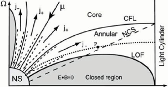
Figure 1.— Sketch for the annular gap and the core gap for particle acceleration. CFL stands for the critical field line across the intersection of the null charge surface and the light cylinder, NCS for the null charge surface, and LOF for the last open field line. P is the peak emission spot at a field line in the annular gap region, which is located between CFL and LOF. This figure is taken and revised from Figure 1 of Qiao et al. (2007).

2. The annular gap and core gap

2.1. Formation of the Annular Gap and the Core Gap

The open field line region of pulsar magnetosphere can be divided into two parts by the critical field lines (see Figure 1). The core region near the magnetic axis is defined by the critical field lines. The annular region is located between the critical field lines and the last open field lines. For an anti-parallel rotator the radius of the core gap ($r_{\rm core}$) and the full polar cap region ($r_{\rm p}$) are $r_{\rm core}=(2/3)^{3/4}R(\Omega R/c)^{1/2}$ and $r_{\rm p}=R(\Omega R/c)^{1/2}$, respectively (Ruderman & Sutherland, 1975), where $R$ is the neutron star radius, $\Omega$ is the angular velocity ($\Omega=2\pi/P$, $P$ is the pulsar spin period). The radius of the annular polar region therefore is $r_{\rm ann}=r_{\rm p}-r_{\rm core}=0.26R(\Omega R/c)^{1/2}$. It is larger for pulsars with smaller spin periods.

The annular acceleration region is negligible for older long period pulsars, but very important for pulsars with a small period, e.g., millisecond pulsars and young pulsars. It extends from the pulsar surface to the null charge surface or even beyond it (see Figure 1). The annular gap has a sufficient thickness of trans-field lines and a wide altitude range for particle acceleration. In the annular gap model, the high energy emission is generated in the vicinity of the null charge surface (Du et al., 2010). This leads to a fan-beam $\gamma$-ray emission (Qiao et al., 2007). The radiation from both the core gap and the annular gap can be observed by one observer (Qiao et al., 2004b) if the inclination angle and the viewing angle are suitable.

2.2. Acceleration Electric Field

The charged particles can not co-rotate with a neutron star near the light cylinder and must escape from the magnetosphere. If particles escape near the light cylinder, these particles have to be generated and move out from the inner region to the outer region. This dynamic process is always taking place, and a huge acceleration electric field exists in the magnetosphere. To keep the whole system charge-free, the neutron star surface must supply the charged particles to the magnetosphere.

The annular gap and the core gap have particles with opposite sign flowing, which can lead to the circuit closure in the whole magnetosphere. The potential along the closed field lines and the critical field lines are different (Xu et al., 2006). The parallel electric fields ($E_{\parallel}$) in the annular gap and core gap regions are opposite, as has been discussed by Sturrock (1971). As a result, $E_{\parallel}$ vanishes at the boundary (i.e. the critical field lines) between the annular and the core regions and also along the closed field lines. The positive and the negative charges are accelerated from the core and the annular regions, respectively.

Figure 2.— For the Vela pulsar, the acceleration electric field is calculated along the field line marked as the dotted line with ‘P’ in Figure 1 with a magnetic azimuthal $\psi=0^{\circ}$ and a magnetic inclination angle $\alpha=70^{\circ}$ in the annular gap model.

We now consider a tiny magnetic tube in the annular gap region. We assume that the particles flow out at a radial distance about $r_{\rm out}\sim R_{\rm LC}=4.3\;10^{3}$ km, and that the charge density of flowing-out particles $\rho_{\rm b}(r_{\rm out})$ is equal to the local Goldreich-Julian (GJ) charge density $\rho_{\rm gj}(r_{\rm out})$ (Goldreich & Julian, 1969) at a radial distance of $r_{\rm out}$. For any heights $r<r_{\rm out}$, $\rho_{\rm b}(r)<\rho_{\rm gj}(r)$. The acceleration electric field therefore exists along the field line, and cannot vanish until approaching the height of $r_{\rm out}$.

For a static dipole magnetic field, the field components can be described as $\mathbf{B}_{r}=\frac{2\mu\cos\theta}{r^{3}}\mathbf{n}_{r}$ and $\mathbf{B}_{\theta}=\frac{\mu\sin\theta}{r^{3}}\mathbf{n}_{\theta}$, here $\theta$ is the zenith angle in magnetic field coordinate, and $B_{0}$ is the surface magnetic field. Thus the magnetic field at a height $r$ is $B(r)=\frac{B_{0}R^{3}}{2}\frac{\sqrt{3\cos^{2}\theta+1}}{r^{3}}$. In the co-rotating frame, Poisson’s equation is

$$\nabla\cdot\mathbf{E}=4\pi(\rho_{\rm b}-\rho_{\rm gj}).$$ (1)

Because of the conservation laws of the particle number and magnetic flux in the magnetic flux tube, the difference between the flowing charge density and local GJ charge density at the radius $r$ can be written as

$$\rho_{\rm b}(r)-\rho_{\rm gj}(r)=-\frac{\Omega B(r)}{2\pi c}(\cos\zeta_{\rm out}-\cos\zeta),$$ (2)

where $\Omega=2\pi/P$ is the angular velocity, $P$ is the rotation period, and $\zeta$ (and $\zeta_{\rm out}$) are the angle between the rotational axis and the $B$ field direction at $r$ (and $r_{\rm out}$). Wang et al. (2006) found

$$\cos\zeta=\cos\alpha\cos\theta_{\mu}-\sin\alpha\sin\theta_{\mu}\cos\psi,$$ (3)

where $\psi$ and $\theta_{\mu}$ are the azimuthal angle and the tangent angle (half beam angle) in the magnetic field coordinate, respectively. Combining equations (1), (2) and (3), we obtain

$$\nabla\cdot{\rm\bf E}=-\frac{\Omega B_{0}R^{3}}{cr^{3}}{\sqrt{3\cos^{2}\theta+1}}(\cos\zeta_{\rm out}-\cos\zeta).$$ (4)

Substituting $\cot\theta_{\mu}=\frac{2\cot^{2}\theta-1}{3\cot\theta}$ (Qiao & Lin, 1998) and $ds=\sqrt{(rd\theta)^{2}+(dr)^{2}}$ into equations (3) and (4), We can solve the equation for $\nabla\cdot\mathbf{E}$, and calculate the electric field $E_{\parallel}$ along a magnetic filed line for $\psi=0^{\circ}$, as shown in Figure 2 for the Vela pulsar. The electric field is huge in the inner region of annular gap and drops quickly when $r\sim R_{\rm LC}$.

3. Modeling the Fermi $\gamma$-ray profiles and spectra of the Vela pulsar

We reprocessed the Fermi data to obtain the multi-band light curves in the following steps: (1) Limited by the timing solution for the Vela pulsar from the Fermi Science Support Center (FSSC), we reprocessed the original data observed from 2008 August 4 to 2009 July 2. (2) We selected photons of 0.1-300 GeV in the “Diffuse” event class, within a radius of $2^{\circ}$ of the Vela pulsar position (RA$=128.55^{\circ}$, DEC$=-45.75^{\circ}$) and the zenith angle smaller than $105^{\circ}$. (3) As done by Abdo et al. (2009, 2010b, 2010c), we used “fselect” to select photons of energy $E_{\rm GeV}$ within an angle of $<\max[1.6-3\log_{10}(E_{\rm GeV}),1.3]$ degrees from the pulsar position. (4) Using the tempo2 (Hobbs et al., 2006; Edwards et al., 2006) with the Fermi plug-in, we obtained the rotational phase for each photon. (5) Finally we obtained the multi-band $\gamma$-ray light curves with 256 bins, as presented in Figure 4 (red solid lines). Two sharp peaks have a phase separation of $\delta\phi\sim 0.42$. The ratio of P2/P1 increases with energy. A third broad peak appears in the bridge emission. The intensity and phase location of P3 vary with energy.

These observed features challenge all current high energy emission models. A convincing model with reasonable input parameters for magnetic inclination angle $\alpha$ and viewing angle $\zeta$ should produce multi-band light curves of the Vela pulsar and explain the energy-dependent location of P3 as well as the ratio of P2/P1.

3.1. Geometric Modeling the Light Curves

Model parameters for both the annular gap and core gap of the Vela pulsar should be adjusted for the particle acceleration regions where the $\gamma$-ray emission are generated. The framework of the annular gap model as well as the coordinate details have been presented in Du et al. (2010), which can be used for simulation of the multi-band $\gamma$-ray light curves of the Vela pulsar. In this paper, we added the simulations for the core gap to explain P3 and bridge emission. We adopted the inclination angle of $\alpha=70^{\circ}$ and the viewing angle $\zeta=64^{\circ}$ which were obtained from the X-ray torus fitting (Ng & Romani, 2008). The modeling was done as follows.

1. We first separate the polar cap region into the annular and core gap regions by the critical field line. Then, we use the so-called “open volume coordinates” ($r_{\rm OVC},\psi_{\rm s}$) to label the open field lines for the annular gap and core gap, respectively. Here $r_{\rm OVC}$ is the normalized magnetic colatitude and $\psi_{\rm s}$ is the magnetic azimuthal. We define $\psi_{\rm s}=0$ for the plane of the magnetic axis and the spin axis, shown in Figure 1. For the annular gap, we define the inner rim $r_{\rm OVC,\,AG}\equiv 0$ for the critical field lines and the outer rim $r_{\rm OVC,\,AG}\equiv 1$ for the last open field lines; while for the core gap, we define the outer rim $r_{\rm OVC,\,CG}\equiv 1$ for the critical field lines and the inner rim $r_{\rm OVC,\,CG}\equiv 0$ for the magnetic axis. We also divide both the annular gap ($0\lesssim r_{\rm OVC,\,AG}\lesssim 1$) and the core gap ($0.1\lesssim r_{\rm OVC,\,CG}\lesssim 1$) into 40 rings for calculation.

Figure 3.— The height of the emission peak $r_{\rm p}$ of the Vela pulsar in the annular gap model and the height of null charge surface $r_{\rm N}$, calculated with an incliantion angle $\alpha=70^{\circ}$, $\kappa=0.7$ and $\lambda=0.9$. Note that $r_{\rm p}$ and $r_{\rm N}$ are symmetric around the magnetic axis in the magnetic frame. The projected $r_{\rm p}$ is always within the light cylinder. We define $\psi_{\rm s}=0^{\circ}$ for the median between the magnetic axis and the equator in the plane of the spin axis and magnetic axis.

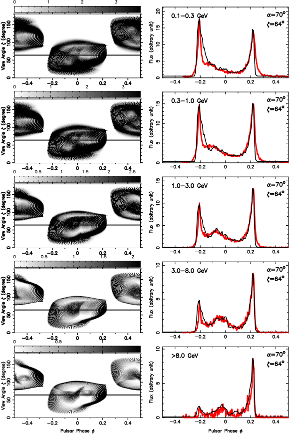
Figure 4.— The observed multi-band $\gamma$-ray light curves of the Vela pulsar (thick red lines in the right panels) and simulated profiles from our model (thin black lines). P1 and P2 comes from the annular gap region, and P3 and bridge emission from the core gap region. The inclination angle $\alpha=70^{\circ}$ and the viewing angle $\zeta=64^{\circ}$ (Ng & Romani 2008) were used for modeling. The line of sight cuts across the $\gamma$-ray emission produced from only one pole. [See the electronic edition of the Journal for a color version of this figure.]

2. Rather following the conventional assumption of the uniform emissivity along an open field line when modeling the light curves (Dyks & Rudak, 2003; Harding et al., 2008; Fang & Zhang, 2010), for both the annular gap and the core gap, we assume that the $\gamma$-ray emissivities $I(\theta_{\rm s},\psi_{\rm s})$ along one open field line have a Gaussian distribution, i.e.,

$$I(\theta_{\rm s},\psi_{\rm s})=I_{\rm P}(\theta_{\rm p},\psi_{\rm s})\exp{\Bigg{[}-\frac{\Big{(}C(\theta_{\rm s},\psi_{\rm s})-C_{\rm 0}(\theta_{\rm p},\psi_{\rm s})\Big{)}^{2}}{2\sigma_{\rm A}^{2}}\Bigg{]}},$$ (5)

here $\theta_{\rm s}$ is the magnetic colatitude of a spot on a field line, $\psi_{\rm s}$ is the magnetic azimuthal of this field line, $C(\theta_{\rm s},\psi_{\rm s})=\int_{0}^{\theta_{\rm s}}\sqrt{r^{2}+({\rm d}r/{\rm d\theta})^{2}}\,\rm d\theta$ is the arc length of the emission point on each field line counted from the pulsar center, $\sigma_{\rm A}$ is a length scale for the emission region on each open field line in the annular gap or the core gap in units of $R_{\rm LC}$, and $C_{\rm 0}(\theta_{\rm p},\psi_{\rm s})$ is the arc length for the peak emissivity spot P($\theta_{\rm p},\psi_{\rm s}$) on this open field line. In principle, the peak position P($\theta_{\rm p},\psi_{\rm s}$) is dependent on the acceleration electric field and the emission mechanism. Based on our 1-D calculation of the acceleration field (see Figures 2) and later the emissivity (see Figure 8 later), the peak emission comes near the null charge surface. The height $r_{\rm p,AG}$ for emission peak on open field lines can be related to the height of the null charge surface $r_{\rm N}(\psi_{\rm s})$ by

$$r_{\rm p,\,AG}(\psi_{\rm s})=\lambda\kappa r_{\rm N}(\psi_{\rm s})+(1-\lambda)\kappa r_{\rm N}(0),$$ (6)

where $\kappa$ is a model parameter for the ratio of heights, and $\lambda$ is a model parameter describing the deformation of emission location from a circle (see details in Lee et al., 2006). The emission peak position ‘P’ on each field line can be uniquely determined, i.e., $\theta_{\rm p}=\arcsin[{\sqrt{r_{\rm p,\,AG}/R_{\rm e,f}(\alpha,\psi_{\rm s})}}]$, where $R_{\rm e,f}(\alpha,\psi_{\rm s})$ is the field line constant of the open field line with $\psi_{\rm s}$. Figure 3 shows the variations of $r_{\rm p,\,AG}\,(\psi_{\rm s})$ and $r_{\rm N}\,(\psi_{\rm s})$ with $\psi_{\rm s}$. The minimum is at $\psi_{\rm s}=0^{\circ}$ near the equator and the maximum at $\psi_{\rm s}=\pm 180^{\circ}$ near the rotation axis.

The peak emissivity $I_{\rm p}(\theta_{\rm P},\psi_{\rm s})$ may follow another Gaussian distribution against $\theta$ for a bunch of open field lines (Cheng et al., 2000; Dyks & Rudak, 2003; Fang & Zhang, 2010), i.e.,

$$I_{\rm P}(\theta_{\rm p},\psi_{\rm s})=I_{\rm 0}\exp{\Bigg{[}-\frac{\Big{(}\theta_{\rm sp}(\psi_{\rm s})-\theta_{\rm cp}(\psi_{\rm s})\Big{)}^{2}}{2\sigma_{\rm\theta}^{2}}\Bigg{]}},$$ (7)

where $I_{\rm 0}$ is a scaled emissivity, $\sigma_{\rm\theta}$ is a bunch scale of $\theta$ (in units of rad) for a set of field lines of the same $\psi_{\rm s}$. $\theta_{\rm sp}$ is used to label a field line in the pulsar annular regions, $\theta_{\rm cp}=(\theta_{\rm N,\psi_{\rm s}}+\theta_{\rm p,\psi_{\rm s}})/2$ (i.e. $r_{\rm ovc}\,(\psi_{\rm s})=0.5$) is the central field line among those field lines with $\psi_{\rm s}$.

As seen above, we use two different Gaussian distributions to describe the emissivity on open field lines for both the annular gap and the core gap. The model parameters are independently adjusted to maximally fit the observed $\gamma$-ray light curves. In the core gap, we assume that the height of emission peak $r_{\rm p,\,CG}=\varepsilon\cdot r_{\rm p,\,AG}$, where $\varepsilon$ is a model parameter. We adopted two different $\sigma_{\rm\theta,C}$ for the core gap because of the different acceleration efficiencies for field lines in the two ranges of $\psi_{\rm s}$. We will write $\sigma_{\rm\theta,\,A}$ for the annular region and $\sigma_{\rm\theta,\,C}$ for the core region.

3. To derive the “photon sky-map” in the observer frame, we first calculate the emission direction of each emission spot ${\bf n_{\rm B}}$ in the magnetic frame; then use a transformation matrix $T_{\rm\alpha}$ to transform ${\bf n_{\rm B}}$ into ${\bf n_{\rm spin}}$ in the spin frame; finally use an aberration matrix to transform ${\bf n_{\rm spin}}$ to ${\bf n_{\rm observer}}=\{{\bf n_{\rm x},\,n_{\rm y},\,n_{\rm z}}\}$ in the observer frame. Here $\phi_{\rm 0}=\arctan({\bf n_{\rm y}}/{\bf n_{\rm x}})$ and $\zeta=\arccos({\bf n_{\rm z}}/\sqrt{{\bf n_{\rm x}}^{2}+{\bf n_{\rm y}}^{2}+{\bf n_{\rm z}}^{2}})$ are the rotation phase (without retardation effect) of the emission spot with respect to the pulsar rotation axis and the viewing angle for a distant, nonrotating observer. The detailed calculations for the aberration effect can be found in Lee et al. (2010).

4. We add the phase shift $\delta\phi_{\rm ret}$ caused by the retardation effect, so that the emission phase is $\phi=\phi_{\rm 0}-\delta\phi_{\rm ret}$. Here is no minus sign for $\phi_{\rm 0}$ beacause of the different coordinate systems between our model and the outer gap model (Romani & Yadigaroglu, 1995).

Table 1Model parameters for multi-band $\gamma$-ray light curves of the Vela pulsar

GeV band	$\kappa$	$\lambda$	$\epsilon$	$\sigma_{\rm A}$	$\sigma_{\rm\theta,\,A}$	$\sigma_{\rm\theta,\,C1}$	$\sigma_{\rm\theta,\,C2}$
0.1–0.3	0.68	0.9	1.17	0.5	0.0035	0.0053	0.009
0.3–1.0	0.70	0.9	1.20	0.5	0.0035	0.0046	0.009
1.0–3.0	0.72	0.9	1.15	0.5	0.0014	0.0064	0.01
3.0–8.0	0.72	0.9	0.88	0.5	0.0007	0.0085	0.006
$>$8.0	0.73	0.9	0.82	0.1	0.00085	0.007	0.003

^aThe bunch scale for field lines in the annular gap.
^bThe bunch scale for field lines of $90^{\circ}<\psi_{\rm s}<180^{\circ}$ in the core gap.
^cThe bunch scale for field lines of $-180^{\circ}<\psi_{\rm s}<90^{\circ}$ in the core gap.

5. The “photon sky-map”, defined by the binned emission intensities on the ($\phi$, $\zeta$) plane, can be plotted for 256 bins (see Figure 4). The corresponding light curves cut by a line of sight with a viewing angle $\zeta=64^{\circ}$ are therefore finally obtained. For the viewing angle $\zeta=64^{\circ}$, any magnetic inclination angles of $\alpha$ between $60^{\circ}$ and $75^{\circ}$ in the annular gap model can produce light curves with two sharp peaks and a large peak separation (e.g., 0.4 – 0.5), similar to the observed ones. The emission from the single pole is favored for the Vela pulsar in our model.

The modeled light curves are presented in Figure 4 (black solid lines), with the model parameters listed in Table 1. Emission of P1 and P2 comes from the annular gap region in the vicinity of the null charge surface, and P3 and bridge emission comes from the core gap region. The higher energy P3 emission ($>3$ GeV) comes from lower height, whereas the lower energy $\gamma$-ray emission comes from a higher region. In the annular gap region, higher energy emission is mostly generated in higher region. Nevertheless, the $\gamma$-ray emission heights are above the lower bound of the height determined by $\gamma-B$ absorption (Lee et al., 2010).

The peak emission comes from different field lines and emission heights in the annular gap. The deformation of radiation beam is related to high value of geometric factor $\lambda$ as discussed in Du et al. (2010). Owing to the aberration and retardation effects, the enhanced gamma-ray emission in the outer rim of photon sky-map make the peak very sharp, especially for P2. For the Vela pulsar, the high inclination angle of about $\alpha=70^{\circ}$ is important to get the observed two sharp peaks with a large separation.

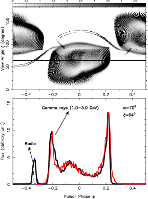
Figure 5.— The jointly modeled radio and $\gamma$-ray light curves (black solid lines) for the Vela pulsar. The radio emission is prodeuced from a higher and narrower region in the annular gap region of the same magnetic pole as the $\gamma$-ray. The observed radio profile (blue dashed line) for the Vela pulsar is taken from the website http://fermi.gsfc.nasa.gov/ssc/data/access/lat/ephems/, and the $\gamma$-ray profile is observed by the Fermi. [See the electronic edition of the Journal for a color version of this figure.]

3.2. Radio Lag

With well-coordinated efforts for pulsar timing program, Abdo et al. (2010c) determined the phase lag between radio emission and $\gamma$-ray light curves. The radio pulse comes earlier by a phase of $\sim 0.13$ (see Figure 5).

Radio emission might be generated in the two locations of a pulsar magnetosphere. One is the traditional low-height polar cap region for long-period ($P\sim 1$s) pulsars (Ruderman & Sutherland, 1975). The other is the outer magnetospheric region with high altitudes near the light cylinder (Manchester, 2005). For the polar cap region, the low radio emission height leads to a small beam, which probably does not point to an observer for the Vela pulsar. Ravi et al. (2010) propose that the radio emission from young pulsars is radiated in a high region close to the null-charge surface, i.e. the similar region for $\gamma$-ray emission. This is somehow similar to our annular gap model, in which the radio emission originates from a higher and narrower region than that of the $\gamma$-ray emission.

The modeled radio and $\gamma$-ray light curves in the two-pole annular gap model are shown in Figure 5. The region for the radio emission is mainly located at a height of $\sim R_{\rm LC}$ on certain filed lines with $\psi_{s}=-138^{\circ}$. Our scenario of radio emission for the Vela pulsar is consistent with the narrow stream of hollow-cone-like radio emission (Dyks et al., 2010). According to our model, not all $\gamma$-ray pulsars can be detected in the radio band, and not all radio pulsars can have a $\gamma$-ray beam towards us.

3.3. $\gamma$-ray Spectra for the Vela Pulsar

Abdo et al. (2010b) got high quality phase-resolved spectra (P1, P2, low-energy P3 and high-energy P3) and the phase-averaged spectrum of the Vela pulsar. The observed $\gamma$-ray emission is believed to originate from the curvature radiation of primary particles (Tang et al., 2008; Harding et al., 2008; Meng et al., 2008). Here we use the synchro-curvature radiation from primary particles (Zhang & Cheng, 1995; Cheng & Zhang, 1996; Meng et al., 2008) and also the synchrotron radiation from secondary particles to calculate the $\gamma$-ray phase-averaged and phase-resolved spectra of the Vela pulsar.

We divide the annular gap region into 40 rings and 360 equal intervals in the magnetic azimuth, i.e. in total 40$\times$360 small magnetic tubes. A small magnetic tube has a small area $A_{0}$ on the neutron star surface. From equation (2), the number density of primary particles at a height $r$ is $n(r)=\frac{\Omega B(r)}{2\pi c\;e}\cos\zeta_{\rm out}$, where $c$ is the speed of light, and $e$ is the electric charge. The cross-section area of the magnetic tube at $r$ is $A(r)=B_{0}A_{0}/B(r)$. Therefore, the flowing particle number at $r$ in the magnetic tube is

$$\Delta N(r)=A(r)\Delta s\frac{\Omega B(r)}{2\pi ce}\cos\zeta_{\rm out},$$ (8)

here $\Delta s$ is the arc length along the field.

The accelerated particles are assumed to flow along a field line in a quasi-steady state. Using the calculated acceleration electric field shown in Figure 2, we can obtain the Lorentz factor $\gamma$ of the primary particle from the curvature radiation reaction

$$\gamma=(\frac{3\rho^{2}E_{\parallel}}{2e})^{\frac{1}{4}}=2.36\times 10^{7}{\rho_{7}}^{0.5}E_{\parallel,\,6}^{0.25},$$ (9)

where $\rho_{7}$ is the curvature radius in units of $10^{7}$ cm and $E_{\parallel,\,6}$ is the acceleration electric field in units of $10^{6}\rm V\,cm^{-1}$. The pitch angle $\beta$ of the primary particles flowing along a magnetic field line is (Meng et al., 2008)

$$\sin\beta\approx\beta\approx\eta\frac{\gamma m_{\rm e}c^{2}}{eB(r)\rho},$$ (10)

where $\eta\leq 1$, $m_{\rm e}$ is the electron mass, and $\rho$ is the curvature radius. The characteristic energy $E_{\rm c}^{\rm syn-cur}$ of synchro-curvature radiation (Zhang & Cheng, 1995; Meng et al., 2008) is given by

$$E {}_{\rm c}^{\rm syn-cur}=\frac{3}{2}\hbar c\gamma^{3}\frac{1}{\rho}$$

$$\times \sqrt{(\frac{r_{\rm B}}{\rho}+1-3\frac{\rho}{r_{\rm B}})\cos^{4}\beta+3\frac{\rho}{r_{\rm B}}\cos^{2}\beta+\frac{\rho^{2}}{r_{\rm B}^{2}}\sin^{4}\beta},$$

where $r_{\rm B}=\frac{\gamma m_{\rm e}c^{2}\sin\beta}{eB(r)}$ is the cyclotron radius of an electron, and $\hbar$ is the reduced Planck constant.

The energy spectrum ${\rm d}N/{\rm d}\gamma$ of the accelerated primary particles is unknown. Harding et al. (2008) have assumed it to follow a broken power-law distribution for pairs with indexes of $-2.0$ and $-2.8$ [see their equation (47)]. Here we assume the primary particles in the magnetic tube to follow one power law ${\rm d}N/{\rm d}\gamma=N_{\rm 0}\gamma^{\Gamma}$ with an index of $\Gamma=-2.4$. Here, $N_{\rm 0}$ can be derived by integration the equation above using the equations (8) and (9). The $\gamma$-ray spectrum emitted by the primary particle can be calculated by (Meng et al., 2008)

$$F (E_{\gamma})=\frac{E_{\rm\gamma}^{2}}{\Delta\Omega d^{2}}\frac{{\rm d}^{2}N_{\gamma}}{{\rm d}E_{\gamma}{\rm d}t}=\frac{\sqrt{3}e^{2}}{2h\Delta\Omega d^{2}}\int_{\gamma_{\rm min}}^{\gamma_{\rm max}}\frac{{\rm d}N}{{\rm d}\gamma}E_{\gamma}$$

$$\times \frac{\gamma}{r_{\rm C}}\Bigg{[}\Bigg{(}1+\frac{1}{r_{\rm C}^{2}Q_{2}^{2}}\Bigg{)}xG(x)-\Bigg{(}1-\frac{1}{r_{\rm C}^{2}Q_{2}^{2}}\Bigg{)}xK_{\rm 2/3}(x)\Bigg{]}{\rm d}\gamma,$$

where $\Delta\Omega$ is the solid angle of the $\gamma$-ray beam, $h$ is the Planck constant, $x=E_{\gamma}/E_{\rm c}^{\rm syn-cur}$, $G(x)=\int_{x}^{+\infty}K_{\rm 5/3}(z){\rm d}z$, $K_{\rm 5/3}(z)$ and $K_{\rm 2/3}(x)$ are the modified bessel function with the order of 5/3 and 2/3, and $r_{\rm C}$ and $Q_{2}^{2}$ are given by

$$r_{\rm C}=\frac{c^{2}}{[(r_{\rm B}+\rho)\Omega_{0}^{2}+r_{\rm B}\omega_{\rm B}^{2}]},$$

$$\Omega_{0}=\frac{c\cos\beta}{\rho},\;\;\;\;\omega_{\rm B}=\frac{eB(r)}{\gamma m_{\rm e}c},$$

$${\small Q_{2}^{2}=\frac{1}{r_{\rm B}}\Bigg{(}\frac{r_{\rm B}^{2}+r_{\rm B}\rho-3\rho^{2}}{\rho^{3}}\cos^{4}\beta+\frac{3}{\rho}\cos^{2}\beta+\frac{1}{r_{\rm B}}\sin^{4}\beta\Bigg{)},}$$

respectively.

Table 2Best fit parameters for modeling the phase-averaged spectrum of the Vela pulsar.

	$\psi_{\rm s}\,(^{\circ})$	$R_{\rm e}$	$r$	$\gamma_{\rm min}^{\rm pri}$	$\gamma_{\rm max}^{\rm pri}$	$\Delta\Omega$	$\gamma_{\rm min}^{\rm 2nd}$	$\gamma_{\rm max}^{\rm 2nd}$
P1	-110	1.095	0.62	0.50$\times 10^{7}$	1.79$\times 10^{7}$	0.11	8.45$\times 10^{5}$	1.31$\times 10^{6}$
P2	131	1.278	0.75	0.30$\times 10^{7}$	2.65$\times 10^{7}$	1.05	6.25$\times 10^{5}$	1.75$\times 10^{6}$
P3	-104	1.122	0.28	0.35$\times 10^{7}$	2.40$\times 10^{7}$	1.09	3.05$\times 10^{5}$	1.22$\times 10^{6}$

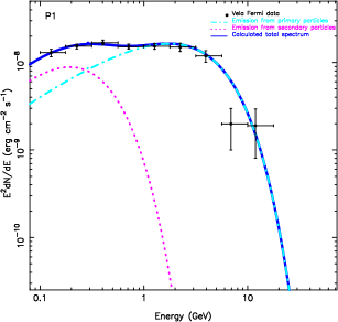
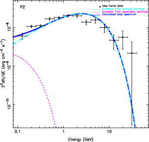
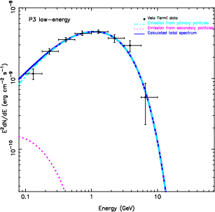
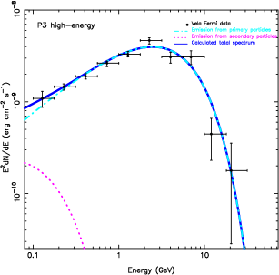
Figure 6.— Fitting the $\gamma$-ray phase-resolved spectra for the Vela pulsar. The observed data were taken from Abdo et al. (2010b) and plotted as black points with error-bars. The contributions of $\gamma$-ray emission from the both primary particles and secondary particles are plotted separately for profile components, P1, P2, P3 low-energy and P3 high-energy. The emission from the secondary particles only partly contribute the lower energy band. [See the electronic edition of the Journal for a color version of this figure.]

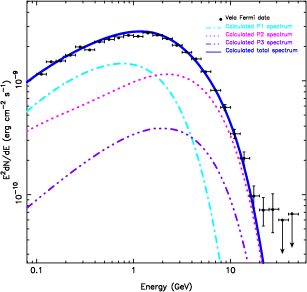
Figure 7.— Fitting the $\gamma$-ray phase-averaged spectrum for the Vela pulsar. The observed data were taken from Abdo et al. (2010b) and plotted as black points with error-bars. The spectra for three profile components and the total phase-averaged spectrum of the Vela pulsar are modeled from the synchro-curvature radiation from primary particles and synchrotron radiation from secondary particles. [See the electronic edition of the Journal for a color version of this figure.]

The secondary particles can be generated with a large multiplicity ($10^{3}-10^{4}$) via the $\gamma-B$ process in the lower regions of the annular gap and the core gap near the neutron star surface. Here, we assume that the energy spectrum of secondary particles follow a power-law, with an index of $\Gamma_{\rm sec}=-2.8$ and a multiplicity of $M_{\rm sec}\sim 1000$. The pitch angle of pairs increase due to the cyclotron resonant absorption of the low-energy photons (Harding et al., 2008). The mean pitch angle of secondary particles is about 0.06, adopted from equation (10) with a slightly large factor $\eta\gtrsim 1$ owing to the effect of cyclotron resonant absorption. The synchrotron radiation from secondary particles have some contributions to the low-energy $\gamma$-ray emission, e.g. $\lesssim 0.3$ GeV.

We further checked the optical depth $\tau_{\rm\gamma-B}$ of the $\gamma-$B absorption (Lee et al., 2010)

$$\tau_{\rm\gamma-B}\,(r)=\frac{1.55\times 10^{7}r}{E_{\rm\gamma}}K_{1/3}^{2}(\frac{2.76\times 10^{6}r^{5/2}P^{1/2}}{B_{\rm 0,\,12}R^{3}E_{\rm\gamma}}),$$ (13)

here $E_{\rm\gamma}$ is in units of MeV, $B_{\rm 0,\,12}$ is in units of $10^{12}$ G. We found that the Fermi $\gamma$-photons of the Vela pulsar with an energy of $<50$ GeV always have a $\tau_{\rm\gamma-B}\ll 1$ if the emission height is greater than a few hundred kilometers.

To reduce the computation time, we calculate the synchro-curvature radiation at the “averaged emission-height” for three components, P1, P2 and P3, of the $\gamma$-ray light curve of the Vela pulsar. For P1, the emission height is about $0.62R_{\rm LC}$ on the field line of a magnetic azimuth $\psi=-110^{\circ}$; for P2, the emission height is $0.75R_{\rm LC}$ on the field line of $\psi=131^{\circ}$; and for P3, the emission height is about $0.28R_{\rm LC}$ on the field line of $\psi=-104^{\circ}$. We compute $E_{\parallel}$ for the three peaks, and adjust the minimum and maximum Lorentz factor for primary particles, $\gamma_{\rm min}^{\rm pri}$ and $\gamma_{\rm max}^{\rm pri}$, and the minimum and maximum Lorentz factor for secondary particles, $\gamma_{\rm min}^{\rm 2nd}$ and $\gamma_{\rm max}^{\rm 2nd}$, and the $\gamma$-ray beam angle $\Delta\Omega$ to fit the $\gamma$-ray spectra for the Vela pulsar.

We fitted the phase-averaged spectrum and phase-resolved (P1, P2, low-energy P3 and high-energy P3) spectra of the Vela pulsar as shown in Figure 6 and Figure 7. The best fit parameters for phase-resolved and phase-averaged spectra are similar as expected, and are listed in Table 2. The maximum Lorentz factor of primary particles $\gamma_{\rm max}^{\rm pri}$ is consistent with that obtained from the curvature radiation balance of the outer magnetosphere models given by Abdo et al. (2010b). The modeled spectra are not sensitive to $\gamma_{\rm min}^{\rm pri}$ or $\gamma_{\rm min}^{\rm 2nd}$, but quite sensitive to $\gamma_{\rm max}^{\rm pri}$ which is chosen around the value of the steady Lorentz factor given by equation (9). The solid angle $\Delta\Omega$ was always assumed to be 1 by many authors for simplicity. We adjusted it as a free parameter around 1 for different phases.

The synchro-curvature radiation from primary particles is the main origin of the observed $\gamma$-ray emission, while the synchrotron radiation from secondary particles can contribute to the lower energy band to improve the fitting. The peak ratios of P1 and P2 shown in Figure 7 are roughly consistent with observations except for the band of 0.3–1.0 GeV (cf. Figure 4). The high-energy P3 is generated in the relatively low height of the core gap, where the particles have a higher acceleration efficiency than those for the low-energy P3, which lead to their cutoff energy different. The phase-resolved spectra for both high-energy P3 and low-energy P3 can be explained in the synchro-curvature radiation from primary particles from the core gap, with little contribution from the synchrotron radiation of secondary particles because they in general have small pitch angles with respect to field lines and large curvature radius. However, the synchrotron radiation from secondary particles does contribute to the $0.1-0.3\,$GeV band for P1 and P2.

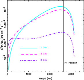
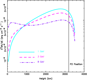
Figure 8.— The emission at 1  3 and 8 GeV for the P1 (top pannel) and P2 (bottom pannel) is not uniform along open field lines. It varies with the height. [See the electronic edition of the Journal for a color version of this figure.]

In Figure 8, we plot the emission fluxes of P1 and P2 component at 1, 3 and 8 GeV of the Vela pulsar against the emission height. It is not uniform along an open field line. The bump at a low height for high energy $\gamma$-ray (e.g. $\gtrsim$8 GeV) due mainly to the small curvature radius and large acceleration electric field there. In Section 3.1, we roughly took a Gaussian distribution along the arc (equation 5) to decribe the emissivity near the peak emission region, which is natural in our annular gap model and independent of the model paranmeters.

4. Discussions and Conclusions

The detailed features of $\gamma$-ray pulsed emission of the Vela pulsar observed by Fermi provide challenge to current emission models for pulsars.

The charged particles can not co-rotate with a neutron star near the light cylinder, and must flow out from the magnetosphere. To keep the whole system charge-free, the neutron star surface must have the charged particles flowing into the magnetosphere. We found that the acceleration electric field $E_{\parallel}$ in a pulsar magnetosphere is strongly correlated with the GJ density $\rho_{\rm gj}$ near the light cylinder radius $R_{\rm LC}$, while $\rho_{\rm gj}$ at $(R_{\rm LC})$ is proportional to the local magnetic field $B_{\rm LC}$. It has been found that the Fermi $\gamma$-ray pulsars can be young pulsars and millisecond pulsars which have a high $B_{\rm LC}$. This means that the acceleration electric field $E_{\parallel}$ in a pulsar magnetosphere is related to the observed Fermi $\gamma$-ray emission from pulsars.

To well understand the multi-band pulsed $\gamma$-ray emission from pulsars, we considered the magnetic field configuration and 3-D global accleration electric field with proper boundary conditions for the annular gap and the core gap. We developed the 3D annular gap model combined with a core gap to fit the $\gamma$-ray light curves and spectra. Our results can reproduce the main observed features for the Vela pulsar. The emission peaks, P1 and P2, originate from the annular gap region, and the P3 and bridge emission comes from the core gap region. The location and intensity of P3 are related to the emission height in the core region. The higher energy emission ($>3$ GeV) comes from lower regions below the null charge surface, while the emission of lower energy of less than 3 GeV comes from the region near or above the null charge surface. Radio emission originates from a region, higher and narrower than those for the $\gamma$-ray emission, which explains the phase lag of $\sim 0.13$ prior to P1, consistent with the model proposed by Dyks et al. (2010).

Synchro-curvature radiation is a effective mechanism for charged particles to radiate in the generally curved magnetic field lines in pulsar magnetosphere (Zhang & Cheng, 1995; Cheng & Zhang, 1996). The GeV band emission from pulsars is originated mainly from curvature radiation from primary particles, while synchrotron radiation from secondary particles have some contributions to the low-energy $\gamma$-ray band (e.g., $0.1-0.3$ GeV). Moreover, contributions of curvature radiation from secondary particles and inverse Compton scattering from both primary particles and secondary particles could be ignored in the $\gamma$-ray band. The synchro-curvature radiation from the primary particles and synchrotron radiation from secondary particles are calculated to model the phase-resolved spectra for P1, P2 and P3 of low-energy band and high-energy band and the total phase-averaged $\gamma$-ray spectrum.

In short, the $\gamma$-ray emission from the Vela pulsar can be well modeled with the annular gap and core gap.

References

- Abdo et al. (2009) Abdo, A. A., et al. 2009, ApJ, 696, 1084
- Abdo et al. (2010a) Abdo, A. A., et al. 2010a, ApJ, 713, 146
- Abdo et al. (2010b) Abdo, A. A., et al. 2010b, ApJ, 713, 154
- Abdo et al. (2010c) Abdo, A. A., et al. 2010c, ApJS, 187, 460
- Abdo et al. (2010d) Abdo, A. A., et al. 2010d, ApJ, 720, 272
- Arons (1983) Arons, J. 1983, ApJ, 266, 215
- Cheng et al. (1986a) Cheng, K. S., Ho, C., & Ruderman, M. 1986a, ApJ, 300, 500
- Cheng et al. (1986b) Cheng, K. S., Ho, C., & Ruderman, M. 1986b, ApJ, 300, 522
- Cheng & Zhang (1996) Cheng, K. S., & Zhang, J. L. 1996, ApJ, 463, 271
- Cheng et al. (2000) Cheng, K. S., Ruderman, M., & Zhang, L. 2000, ApJ, 537, 964
- Daugherty & Harding (1994) Daugherty, J. K., & Harding, A. K. 1994, ApJ, 429, 325
- Daugherty & Harding (1996) Daugherty, J. K., & Harding, A. K. 1996, ApJ, 458, 278
- Dodson et al. (2003) Dodson, R., Legge, D., Reynolds, J. E., & McCulloch, P. M. 2003, ApJ, 596, 1137
- Du et al. (2010) Du, Y. J., Qiao, G. J., Han, J. L., Lee, K. J., Xu, R. X. 2010, MNRAS, 406, 2671
- Dyks & Rudak (2003) Dyks, J., & Rudak, B. 2003, ApJ, 598, 1201
- Dyks et al. (2010) Dyks, J., Rudak, B., & Demorest, P. 2010, MNRAS, 401, 1781
- Edwards et al. (2006) Edwards, R. T., Hobbs, G. B., & Manchester, R. N. 2006, MNRAS, 372, 1549
- Fang & Zhang (2010) Fang, J., & Zhang, L. 2010, ApJ, 709, 605
- Fierro et al. (1998) Fierro, J. M., Michelson, P. F., Nolan, P. L., & Thompson, D. J. 1998, ApJ, 494, 734
- Gangadhara (2005) Gangadhara, R. T. 2005, ApJ, 628, 923
- Goldreich & Julian (1969) Goldreich, P., & Julian, W. H. 1969, ApJ, 157, 869
- Grenier et al. (1988) Grenier, I. A., Hermsen, W., & Clear, J. 1988, A&A, 204, 117
- Harding et al. (2008) Harding, A. K., Stern, J. V., Dyks, J., & Frackowiak, M. 2008, ApJ, 680, 1378
- Hirotani (2008) Hirotani, K. 2008, ApJ, 688, L25
- Hobbs et al. (2006) Hobbs, G. B., Edwards, R. T., & Manchester, R. N. 2006, MNRAS, 369, 655
- Kanbach et al. (1994) Kanbach, G., et al. 1994, A&A, 289, 855
- Lee et al. (2006) Lee, K. J., Qiao, G. J., Wang, H. G., & Xu, R. X. 2006, Advances in Space Research, 37, 1988
- Lee et al. (2010) Lee, K. J., Du, Y. J., Wang, H. G., Qiao, G. J., Xu, R. X., & Han, J. L. 2010, MNRAS, 405, 2103
- Lin & Zhang (2009) Lin, G. F., & Zhang, L. 2009, ApJ, 699, 1711
- Lommen et al. (2007) Lommen, A., et al. 2007, ApJ, 657, 436
- Lu et al. (1994) Lu, T., Wei, D. M., & Song, L. M. 1994, A&A, 290, 815
- Manchester (2005) Manchester, R. N. 2005, Ap&SS, 297, 101
- Manchester et al. (2005) Manchester, R. N., Hobbs, G. B., Teoh, A., & Hobbs, M. 2005, AJ, 129, 1993
- Meng et al. (2008) Meng, Y., Zhang, L., & Jiang, Z. J. 2008, ApJ, 688, 1250
- Muslimov & Harding (2003) Muslimov, A. G., & Harding, A. K. 2003, ApJ, 588, 430
- Muslimov & Harding (2004) Muslimov, A. G., & Harding, A. K. 2004, ApJ, 606, 1143
- Ng & Romani (2008) Ng, C.-Y., & Romani, R. W. 2008, ApJ, 673, 411
- Pellizzoni et al. (2009) Pellizzoni, A., et al. 2009, ApJ, 691, 1618
- Pellizzoni et al. (2010) Pellizzoni, A., et al. 2010, Science, 327, 663
- Qiao & Lin (1998) Qiao, G. J., & Lin, W. P. 1998, A&A, 333, 172
- Qiao et al. (2004a) Qiao, G. J., Lee, K. J., Wang, H. G., Xu, R. X., & Han, J. L. 2004a, ApJL, 606, L49
- Qiao et al. (2004b) Qiao, G. J., Lee, K. J., Zhang, B., Xu, R. X., & Wang, H. G. 2004b, ApJL, 616, L127
- Qiao et al. (2007) Qiao, G. J., Lee, K. J., Zhang, B., Wang, H. G., & Xu, R. X. 2007, Chinese Journal of Astronomy and Astrophysics, 7, 496
- Ravi et al. (2010) Ravi, V., Manchester, R. N., & Hobbs, G. 2010, ApJ, 716, L85
- Romani & Yadigaroglu (1995) Romani, R. W., & Yadigaroglu, I.-A. 1995, ApJ, 438, 314
- Ruderman & Sutherland (1975) Ruderman, M. A., & Sutherland, P. G. 1975, ApJ, 196, 51
- Sturrock (1971) Sturrock, P. A. 1971, ApJ, 164, 529
- Tang et al. (2008) Tang, A. P. S., Takata, J., Jia, J. J., & Cheng, K. S. 2008, ApJ, 676, 562
- Thompson et al. (1975) Thompson, D. J., Fichtel, C. E., Kniffen, D. A., & Ogelman, H. B. 1975, ApJ, 200, L79
- Thompson et al. (1999) Thompson, D. J., et al. 1999, ApJ, 516, 297
- Thompson (2001) Thompson, D. J. 2001, American Institute of Physics Conference Series, 558, 103
- Wang et al. (2006) Wang, H. G., Qiao, G. J., Xu, R. X., & Liu, Y. 2006, MNRAS, 366, 945
- Xu (2002) Xu, R. X. 2002, ApJL, 570, L65
- Xu (2005) Xu, R. X. 2005, MNRAS, 356, 359
- Xu et al. (2006) Xu, R. X., Cui, X. H., & Qiao, G. J., 2006, Chin. J. Astron. Astrophys. 6, 217
- Yu et al. (2009) Yu, H., Fang, J., & Jiang, Z.-J. 2009, Research in Astronomy and Astrophysics, 9, 1324
- Zhang & Harding (2000) Zhang, B., & Harding, A. K. 2000, ApJ, 532, 1150
- Zhang & Cheng (1995) Zhang, J. L., & Cheng, K. S. 1995, Physics Letters A, 208, 47
- Zhang & Cheng (1997) Zhang, L., & Cheng, K. S. 1997, ApJ, 487, 370
- Zhang et al. (2004) Zhang, L., Cheng, K. S., Jiang, Z. J., & Leung, P. 2004, ApJ, 604, 317
- Zhang et al. (2007) Zhang, L., Fang, J., & Chen, S. B. 2007, ApJ, 666, 1165