INFLECTION POINTS OF REAL AND TROPICAL PLANE CURVES

Abstract.

We prove that Viro’s patchworking produces real algebraic curves with the maximal number of real inflection points. In particular this implies that maximally inflected real algebraic $M$-curves realize many isotopy types. The strategy we adopt in this paper is tropical: we study tropical limits of inflection points of classical plane algebraic curves. The main tropical tool we use to understand these tropical inflection points are tropical modifications.

1. Introduction

Let $k$ be any field of characteristic 0, and consider a plane algebraic curve $X$ in $kP^{2}$ given by the homogeneous equation $P(z,w,u)=0$. The Hessian of the polynomial $P(z,w,u)$, denoted by $Hess_{P}(z,w,u)$, is the homogeneous polynomial defined as

$$Hess_{P}(z,w,u)=\det\left(\begin{matrix}\frac{\partial^{2}P}{\partial^{2}z}\par&$ $&\frac{\partial^{2}P}{\partial z\partial w}\par&$ $&\frac{\partial^{2}P}{\partial z\partial u}\\ $ $&$ $&$ $\\ \frac{\partial^{2}P}{\partial z\partial w}\par&$ $&\frac{\partial^{2}P}{\partial^{2}w}\par&$ $&\frac{\partial^{2}P}{\partial w\partial u}\\ $ $&$ $&$ $\\ \frac{\partial^{2}P}{\partial z\partial u}\par&$ $&\frac{\partial^{2}P}{\partial w\partial u}\par&$ $&\frac{\partial^{2}P}{\partial^{2}u}\par\end{matrix}\right).$$

If $Hess_{P}(z,w,u)$ is not the null polynomial, it defines a curve $Hess_{X}$ called the Hessian of $X$. Note that $Hess_{X}$ only depends on $X$, and is invariant under projective transformations of $kP^{2}$. An inflection point of the curve $X$ is by definition a point $p$ in $X\cap Hess_{X}$, of multiplicity $m$ if $(X\circ Hess_{X})_{p}=m$.

A plane algebraic curve has two kinds of inflection points: its singular points, and non-singular points having a contact of order $l\geq 3$ with their tangent line. In this latter case, the multiplicity of such an inflection point is exactly $l-2$.

If $k$ is algebraically closed, Bézout Theorem implies that an algebraic curve $X$ in $kP^{2}$ of degree $d\geq 2$ which is reduced and does not contain any line has exactly $3d(d-2)$ inflection points (counted with multiplicity). Moreover, a non-singular generic curve $X$ has exactly $3d(d-2)$ inflection points, all of them of multiplicity 1.

When $k$ is not algebraically closed, the situation becomes more subtle. First, the number of inflection points of an algebraic curve in $kP^{2}$ depends not only on its degree, but also on the coefficients of its equation. In the case $k={\mathbb{R}}$, it has been known for a long time that a non-singular real cubic has only 3 real points among its 9 inflection points. More generally, Klein proved that at most one third of the complex inflection points of a non-singular real algebraic curve can actually be real.

Theorem 1.1 (Klein [Kle76a], see also [Ron98], [Sch04], and [Vir88]).

A non-singular real algebraic curve in ${\mathbb{R}}P^{2}$ of degree $d\geq 3$ cannot have more than $d(d-2)$ real inflection points.

Klein also proved that this upper bound is sharp. Following [KS03], we say that a non-singular real algebraic curve of degree $d$ in ${\mathbb{R}}P^{2}$ is maximally inflected if it has $d(d-2)$ distinct real inflexion points. If a real algebraic curve has a node $p$ with two real branches such that each branch is locally strictly convex around $p$, then any smoothing of $p$ produces two real inflection points. Applying Hilbert’s method of construction, the previous observation implies immediately the existence of maximally inflected curves in any degree at least 2. However, real inflection points of maximally inflected curves remains quite mysterious. For example, which rigid-isotopy classes of real algebraic curves contain a maximally inflected curve? How real inflection points can be distributed among the connected component of a maximally inflected curve?

The first step to answer questions of this sort is of course to find a systematic way to construct maximally real inflected curves. Invented by Viro at the end of the seventies (see [Vir82]), the patchworking technique turned out to be one of the most powerful method to construct real algebraic curves with controlled topology. One of the main contribution of this paper is to prove that patchworking also provides a systematic method to construct maximally inflected real curves.

For the sake of shortness we do not recall this technique here, we refer instead to the tropical presentation made in [Vir01], [Mik04], or [Bru09]. In non-tropical terms, Theorem 1 states that any real primitive $T$-curve, under a mild assumption on the corresponding convex function, is maximally inflected. Note that this result is of the same flavor as the fact that $T$-curves have asymptotically maximal total curvature (see [Lop06] and [Ri]). We denote by $T_{d}$ the triangle in ${\mathbb{R}}^{2}$ with vertices $(0,0)$, $(d,0)$ and $(0,d)$. All precise definitions needed in Theorem 1 are given in section 3.

Theorem 1.

Let $C$ be a non-singular tropical curve in ${\mathbb{R}}^{2}$ defined by the tropical polynomial ${\text{``}}\sum_{i,j}a_{i,j}x^{i}y^{j}{\text{''}}$ with Newton polygon the triangle $T_{d}$ with $d\geq 2$. Suppose that if $v$ is a vertex of $C$ dual to $T_{1}$, then its 3 adjacent edges have 3 different length. Then the real algebraic curve defined by the polynomial $P(z,w)=\sum_{i,j}\alpha_{i,j}t^{-a_{i,j}}z^{i}w^{j}$ with $\alpha_{i,j}\in{\mathbb{R}}$ has exactly $d(d-2)$ inflection points in ${\mathbb{R}}P{{}^{2}}$ for $t>0$ small enough.

As an example of application of Theorem 1, combined with classical results in topology of real algebraic curves (see [Vir82] and [Vir84] for example), we get the following corollary.

Corollary 1.

Any rigid isotopy class of non-singular real algebraic curves of degree at most 6 with non-empty real part contains a maximally inflected curve.

Any real scheme with non-empty real part realized by a non-singular real algebraic curve of degree 7 is realized by a maximally inflected curve of degree 7.

Theorem 1 is a weak version of Theorem 5.7: the polynomials $P(z,w)$ are in fact polynomials over the field of generalized Puiseux series, and we give in addition the distribution of real inflection points among the connected components of a real algebraic curve obtained by patchworking. See Figures 17 and 18 from Example 5.8, as well as section 7 for some examples of such patchworkings.

A plane tropical curve $C$ can be thought as a combinatorial encoding of a 1-parametric degeneration of plane complex algebraic curves $X(t)$ (see section 3 for definitions). The main part in the proof of Theorem 1 is then to understand which points of $C$ represent a limit of inflection points of the algebraic curves $X(t)$. Since plane tropical curves are piecewise linear objects, the location of these tropical intersection points is not obvious at first sight, and we need to refine the tropical limit process. Tropical modifications, introduced by Mikhalkin in [Mik06], allow such a refinement.

It follows from Kapranov’s Theorem that the tropicalization $C$ of a family of plane complex algebraic curves $X(t)$ only depends on the first order term in $t$ of the coefficients of the equation of $X(t)$. As rough as it may seem, the curve $C$ keeps track of a non-negligible amount of information about the family $(X(t))$. For example, if $C$ is non-singular, the genus of $X(t)$ is equal to the first Betti number of $C$. However, some information depending on more than just first order terms might be lost when passing from $(X(t))$ to $C$. Tropical modifications refine the tropicalization process, and allows one to recover some information about $(X(t))$ sensitive to higher order terms.

By means of these tropical modifications, we identify a finite number of inflection components on any non-singular tropical curve $C$ (Proposition 5.2). These inflection components are the tropical analogues of inflection points. Using further tropical modifications, we prove that the multiplicity $\mu({\mathcal{E}})$ of such a component ${\mathcal{E}}$ (i.e. the number of inflection points of $X(t)$ which tropicalize in ${\mathcal{E}}$) only depends on the combinatoric of $C$ (Theorem 5.6). Now suppose that $X(t)$ is a family of real algebraic curves. As an immediate consequence, we get that the number of real inflection points of $X(t)$ which tropicalize in ${\mathcal{E}}$ has the same parity

as $\mu({\mathcal{E}})$. In Theorem 5.7, we establish that a generic tropical curve has exactly $d(d-2)$ inflection components with odd multiplicity. Hence Theorem 5.7 together with Klein Theorem imply that $X(t)$ has exactly $d(d-2)$ real inflection points when $t$ is small enough.

At several places in the text, we will see that tropical modifications can also be used to localize a problem. For example, relation between classical and tropical intersections (Proposition 4.5), or intersections between a curve and its Hessian (Theorem 5.7), are reduced to easy local considerations after a suitable tropical modification.

Contents

1. 1 Introduction
2. 2 Convention
3. 3 Standard tropical geometry
   1. 3.1 Non-archimedean amoebas
   2. 3.2 Tropical hypersurfaces
   3. 3.3 Tropical intersection
4. 4 Tropical modifications
   1. 4.1 Example
   2. 4.2 General method
   3. 4.3 The case of plane curves
5. 5 Tropicalization of inflection points
   1. 5.1 Inflection points of curves in $(k^{*})^{2}$
   2. 5.2 Location
   3. 5.3 Multiplicities
   4. 5.4 Application to real algebraic geometry
6. 6 End of the proof of Theorem 5.6
   1. 6.1 Hessian of a primitive polynomial
   2. 6.2 Localization
7. 7 Examples

Acknowledgment: We are grateful to Viatcheslav Kharlamov for pointing us the fact that any smoothing of a real node with two local real convex branches produces two real inflection points, as well as for his simplification of the proof of Proposition 7.1. We are also indebted to Grigory Mikhalkin for many useful discussions about tropical modifications.

Finally, we thank Jean-Jacques Risler and Frank Sottile for their encouragements, as well as Cristhian Garay and the unkonwn referee for many useful comments on preliminary versions of this paper.

A major part of this work has been done during the visit of E.B. at the Universidad Nacional Autónoma de México (Instituo de Matemáticas. Unidad Cuernavaca), and during the Tropical Geometry semester at MSRI in Fall 2009. We thank these institutions for their support and excellent working conditions they offered us. Both authors were partially founded by UNAM-PAPIIT IN-117110 and CONACyT 55084. E.B. is also partially supported by the ANR-09-BLAN-0039-01 and ANR-09-JCJC-0097-01. L.L. is also partially supported by UNAM-DGAPA and Laboratorio Internacional Solomon Lefschetz (LAISLA), asociated to the CNRS (France) and CONACYT (Mexico).

2. Convention

Here we pose once for all some notations and conventions we will use throughout the paper. Almost all of them are commonly used in the literature.

An integer convex polytope in ${\mathbb{R}}^{n}$ is a convex polytope with vertices in ${\mathbb{Z}}^{n}$. The integer volume is the Euclidean volume normalized so that the standard simplex with vertices $0$, $(1,0,\ldots,0)$, $(0,1,0,\ldots,0)$, $\ldots$, $(0,\ldots,0,1)$ has volume 1. That is to say, the integer volume in ${\mathbb{R}}^{n}$ is $n!$ times the Euclidean volume in ${\mathbb{R}}^{n}$. In this paper, we only consider integer volumes. A simplex $\Delta$ in ${\mathbb{R}}^{n}$ will be called primitive if it has volume 1. Equivalently, $\Delta$ is primitive if and only if it is the image of the standard simplex under an element of $GL_{n}({\mathbb{Z}})$ composed with a translation.

Given $d\geq 1$, we denote by $T_{d}$ the integer triangle in ${\mathbb{R}}^{2}$ with vertices $(0,0)$, $(d,0)$, and $(0,d)$.

A facet of a polyhedral complex is a face of maximal dimension.

The letter $k$ denotes an arbitrary field of characteristic 0. Given $P(z)$ a polynomial in $n$ variables over $k$, we denote by $V(P)$ the hypersurface of $(k^{*})^{n}$ defined by $P(z)$. We write $P(z)=\sum a_{i}z^{i}$ with $i=(i_{1},\ldots,i_{n})$, $z=(z_{n},\ldots,z_{n})$, and $a_{i}z^{i}=a_{i}z_{1}^{i_{1}}\ldots z_{n}^{i_{n}}$. The Newton polytope of $P(z)$ is denoted by $\Delta(P)\subset{\mathbb{R}}^{n}$, and given a subset $\Delta^{\prime}$ of $\Delta(P)$, we define the restriction of $P(z)$ along $\Delta^{\prime}$, by

$$P^{\Delta^{\prime}}(z):=\sum_{i\in\Delta^{\prime}\cap{\mathbb{Z}}^{n}}a_{i}z^{i}.$$

If $X$ and $X^{\prime}$ are two algebraic curves in the projective plane $kP^{2}$, the intersection multiplicity of $X$ and $X^{\prime}$ at a point $p\in kP^{2}$ is denoted by $(X\circ X^{\prime})_{p}$.

3. Standard tropical geometry

In this section we review briefly some standard facts about tropical geometry, and we fix the notations used in this paper. For a more educational exposition, we refer, for example, to [Mik06], [IMS07], [RGST05], and [BPS08]. There exist several non-equivalent definitions of tropical varieties in the literature. In this paper, we have chosen for practical reasons to present them via non-archimedean amoebas.

3.1. Non-archimedean amoebas

A locally convergent generalized Puiseux series is a formal series of the form

$$a(t)=\sum_{r\in R}\alpha_{r}t^{r}$$

where $R\subset{\mathbb{R}}$ is a well-ordered set, $\alpha_{r}\in{\mathbb{C}}$, and the series is convergent for $t>0$ small enough. We denote by ${\mathbb{K}}$ the set of all locally convergent generalized Puiseux series. It is naturally a field of characteristic $0$, which turns out to be algebraically closed. An element $a(t)=\sum_{r\in R}\alpha_{r}t^{r}$ of ${\mathbb{K}}$ is said to be real if $\alpha_{r}\in{\mathbb{R}}$ for all $r$, and we denote by ${\mathbb{R}}{\mathbb{K}}$ the subfield of ${\mathbb{K}}$ composed of real series.

Since elements of ${\mathbb{K}}$ are convergent for $t>0$ small enough, an algebraic variety over ${\mathbb{K}}$ (resp. ${\mathbb{R}}{\mathbb{K}}$) can be seen as a one parametric family of algebraic varieties over ${\mathbb{C}}$ (resp. ${\mathbb{R}}$).

The field ${\mathbb{K}}$ has a natural non-archimedean valuation defined as follows:

$$\begin{array}[]{cccc}val:&{\mathbb{K}}&\longrightarrow&{\mathbb{R}}\cup\{-\infty\}\\ &0&\longmapsto&-\infty\\ &\sum_{r\in R}\alpha_{r}t^{r}\neq 0&\longmapsto&-min\{r\mid\alpha_{r}\neq 0\}.\end{array}$$

Note that we call $val$ a valuation, although it is rather the opposite of a valuation for classical litterature. This valuation extends naturally to a map $Val:{\mathbb{K}}^{n}\rightarrow({\mathbb{R}}\cup\{-\infty\})^{n}$ by evaluating $val$ coordinate-wise, i.e. $Val(z_{1},\dots,z_{n})=(val(z_{1}),\dots,val(z_{n}))$. If $X\subset({\mathbb{K}}^{*})^{n}$ is an algebraic variety, $Val(X)\subset{\mathbb{R}}^{n}$ is called the non-archimedean amoeba of $X$.

Example 3.1.

An integer matrix $M\in\mathcal{M}_{n,m}({\mathbb{Z}})$ defines a multiplicative map $\Phi_{M}:({\mathbb{K}}^{*})^{m}\to({\mathbb{K}}^{*})^{n}$. The non-archimedean amoeba of $\Phi_{M}(({\mathbb{K}}^{*})^{m})$ is the vector subspace of ${\mathbb{R}}^{n}$ spanned by the columns of $M$.

Let $X$ be an irreducible algebraic variety of dimension $m$. In this case, Bieri and Groves proved in [BG84] that $Val(X)$ is a finite rational polyhedral complex of pure dimension $m$ (rational means that each of its faces has a direction defined over ${\mathbb{Q}}$). Given a facet $F$ of $Val(X)$, we associate a positive integer number $w(F)$, called the weight of $F$, as follows: pick a point $(p_{1},\ldots,p_{n})$ in the relative interior of $F$, and choose a basis $(e_{1},\ldots,e_{n})$ of ${\mathbb{Z}}^{n}\subset{\mathbb{R}}^{n}$ such that $(e_{1},\ldots,e_{m})$ is a basis of the direction of $F$; denote by $Y_{F}\subset({\mathbb{K}}^{*})^{n}$ the multiplicative translation of $\Phi_{(e_{m+1},\ldots,e_{n})}(({\mathbb{K}}^{*})^{n-m})$ along $(t^{p_{1}},\ldots,t^{p_{n}})$, and define $w(F)$ as the number (counted with multiplicity) of intersection points of $X$ and $Y_{F}$ with valuation $(p_{1},\ldots,p_{n})$. Note that $w(F)$ does not depend on the choice of the point $(p_{1},\ldots,p_{n})$.

Example 3.2.

A matrix $M\in\mathcal{M}_{n,m}({\mathbb{Z}})$ with $Ker\ M=\{0\}$ maps the lattice ${\mathbb{Z}}^{m}$ to a sub-lattice $\Lambda^{\prime}$ of $\Lambda={\mathbb{Z}}^{n}\cap Im\ M$. The weight of the non-archimedean amoeba of $\Phi_{M}(({\mathbb{K}}^{*})^{m})$ is the index of $\Lambda^{\prime}$ in $\Lambda$.

Definition 3.3.

The non-archimedean amoeba of $X$ equipped with the weight function on its facets is called the tropicalization of $X$, and is denoted by $Trop(X)$.

The notion of tropicalization extends naturally to any algebraic subvariety of $({\mathbb{K}}^{*})^{n}$, not necessarily of pure dimension. In this paper, a tropical variety is a finite rational polyhedral complex in ${\mathbb{R}}^{n}$ equipped with a weight function, and which is the tropicalization of some algebraic subvariety of $({\mathbb{K}}^{*})^{n}$.

Example 3.4.

A plane tropical curve, a tropical plane in ${\mathbb{R}}^{3}$, and a tropical curve contained in this tropical plane are depicted in Figures 1a, 1b and 1c.

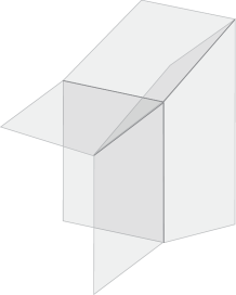
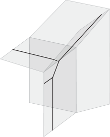
a)	b)	c)

Figure 1. Examples of tropical varieties. In these cases all the weights are equal to 1.

Definition 3.5.

Let $V$ be a tropical variety in ${\mathbb{R}}^{n}$, and $X$ be an algebraic subvariety of $({\mathbb{K}}^{*})^{n}$. We say that $X$ realizes $V$ if $V=Trop(X)$. If $X=V(P)$ for some polynomial $P(z)$, we say that $P(z)$ realizes $V$.

Tropical varieties satisfy the so-called balancing condition. We give here this property only for tropical curves, since this is anyway the only case we need in this paper and makes the exposition easier. We refer to [Mik06] for the general case.

Let $C\subset{\mathbb{R}}^{n}$ be a tropical curve, and let $v$ be a vertex of $C$. Let $e_{1},\ldots,e_{l}$ be the edges of $C$ adjacent to $v$. Since $C$ is a rational graph, each edge $e_{i}$ has a primitive integer direction. If in addition we ask that the orientation of $e_{i}$ defined by this vector points away from $v$, then this primitive integer vector is unique. Let us denote by $u_{v,e_{i}}$ this vector.

Proposition 3.6 (Balancing condition).

For any vertex $v$, one has

$$\sum_{i=1}^{l}w(e_{i})u_{v,e_{i}}=0.$$

If $C$ is a tropical curve in ${\mathbb{R}}^{n}$, any of its bounded edge $e$ has a length $l(e)$ defined as follows:

$$l(e)=\frac{||v_{1}v_{2}||}{w(e)||u_{v_{1},e}||}$$

where $v_{1}$ and $v_{2}$ are its adjacent vertices, and $||v_{1}v_{2}||$ (resp. $||u_{v_{1},e}||$) denotes the Euclidean length of the vector $v_{1}v_{2}$ (resp. $u_{v_{1},e}$).

3.2. Tropical hypersurfaces

Let us now study closer tropical hypersurfaces, i.e. tropical varieties in ${\mathbb{R}}^{n}$ of pure dimension $n-1$. These particular tropical varieties can easily be described as algebraic varieties over the tropical semi-field $({\mathbb{T}},{\text{``}}+{\text{''}},{\text{``}}\times{\text{''}})$. Recall that ${\mathbb{T}}={\mathbb{R}}\cup\{-\infty\}$ and that for any two elements $a$ and $b$ in ${\mathbb{T}}$, one has

${\text{``}}a+b{\text{''}}=\max(a,b)$ and ${\text{``}}a\times b{\text{''}}=a+b.$

As usual, we abbreviate $a\times b$ in $ab$, and $({\mathbb{T}},{\text{``}}+{\text{''}},{\text{``}}\times{\text{''}})$ in ${\mathbb{T}}$, and we use the convention that $\max(-\infty,a)=a$ and $-\infty+a=-\infty$. Note that ${\mathbb{T}}^{*}={\mathbb{R}}$.

Since ${\mathbb{T}}$ is a semi-field, we have a natural notion of tropical polynomials, i.e. polynomials over ${\mathbb{T}}$. Such a polynomial $P(x)={\text{``}}\sum a_{i}x^{i}{\text{''}}$ induces a function

$$\begin{array}[]{cccc}P:&{\mathbb{T}}^{n}&\longrightarrow&{\mathbb{T}}\\ &x&\longmapsto&\max(\left\langle x,i\right\rangle+a_{i})\end{array}$$

where $x=(x_{1},\ldots,x_{n})\in{\mathbb{T}}^{n}$, $i=(i_{1},\ldots,i_{n})\in{\mathbb{N}}^{n}$, $x^{i}={\text{``}}x_{1}^{i_{1}}\ldots,x_{n}^{i_{n}}{\text{''}}$, and $\left\langle\ ,\ \right\rangle$ denotes the standard Euclidean product on ${\mathbb{R}}^{n}$.

We denote by $\overset{\circ}{V}(P)$ the set of points $x$ in ${\mathbb{R}}^{n}$ for which the value of $P(x)$ is given by at least 2 monomials. This is a finite rational polyhedral complex, which induces a subdivision $\Theta$ of ${\mathbb{R}}^{n}$. Given $F$ a face of $\Theta$ and $x$ a point in the relative interior of $F$, the set $\{i\in\Delta(P)\ |\ P(x)={\text{``}}a_{i}x^{i}{\text{''}}\}$ does not depend on $x$. We denote its convex hull by $\Delta_{F}$. All together, the polyhedrons $\Delta_{F}$ form a subdivision of $\Delta(P)$, called the dual subdivision of $P(x)$. The polyhedron $\Delta_{F}$ is called the dual cell of $F$, and $\dim\Delta_{F}=n-\dim F$. In particular, if $F$ is a facet of $\overset{\circ}{V}(P)$ then $\Delta_{F}$ is a segment, and we define the weight of $F$ by $w(F)=Card(\Delta_{F}\cap{\mathbb{Z}}^{n})-1$. We denote by $V(P)$ the polyhedral complex $\overset{\circ}{V}(P)$ equipped with the map $w$ on its facets. $V(P)$ is called the tropical hypersurface defined by $P(x)$.

The Newton polygon of $P(x)$ and its dual subdivision are entirely determined, up to translation, by $V(P)$. A tropical hypersurface is said to be non-singular if all the maximal cells of its dual subdivision are primitive simplices. In particular, any facet of a non-singular tropical hypersurface has weight 1.

Note that we have used the same notations as in section 3.1. This is justified by the following fundamental Theorem, due to Kapranov.

Theorem 3.7 (Kapranov [Kap00]).

Let $P(z)=\sum a_{i}z^{i}$ be a polynomial over ${\mathbb{K}}$. If we define $P_{trop}(x)={\text{``}}\sum val(a_{i})x^{i}{\text{''}}$, then we have

$$Trop(V(P))=V(P_{trop}).$$

Example 3.8.

The tropical planar curve and the tropical plane in Figure 1a and 1b, are given respectively by the tropical polynomials

$P(x,y)={\text{``}}x^{2}+y^{2}+2x+2y+3xy+3{\text{''}}$ and $Q(x,y,z)={\text{``}}x+y+z+1{\text{''}}$.

Let $P(z)$ be a polynomial over ${\mathbb{K}}$ realizing a tropical hypersurface $V$ in ${\mathbb{R}}^{n}$. To each face $F$ of $V$ dual to the polyhedron $\Delta_{F}$, we associate below a complex polynomial $P_{{\mathbb{C}},F}(z)$. Let $i_{1}$, $\ldots$, $i_{l}$ be the vertices of $\Delta_{F}$.

Let us first suppose that $\Delta_{F}$ has dimension $n$. In this case, the points $(i_{1},-val(a_{i_{1}}))$, $\ldots,$ $(i_{l},-val(a_{i_{l}}))$ lie on the same hyperplane in ${\mathbb{R}}^{n}\times{\mathbb{R}}$. Hence we have $-val(a_{i_{j}})=\lambda_{\Delta_{F}}(i_{j})$ where $\lambda_{\Delta_{F}}:{\mathbb{R}}^{n}\to{\mathbb{R}}$ is a linear-affine map. The maps $\lambda_{\Delta_{F}}$ glue along faces of codimension 1 to produce a convex piecewise-affine map $\lambda:\Delta(P)\to{\mathbb{R}}$. Note that the cells of dimension $n$ of the dual subdivision of $V$ correspond exactly to the domains of linearity of $\lambda$, and that $-val(a_{i})\geq\lambda(i)$ for any $i\in\Delta(P)\cap{\mathbb{Z}}^{n}$.

Let us go back to the case when $\Delta_{F}$ may have any dimension between 0 and $n$. According to the preceding paragraph, there exists a linear-affine function $\lambda_{\Delta_{F}}:{\mathbb{R}}^{n}\to{\mathbb{R}}$ such that $-val(a_{i_{j}})=\lambda_{\Delta_{F}}(i_{j})$ for all $j=1\ldots l$, and $-val(a_{i})>\lambda_{\Delta_{F}}(i)$ for any $i$ not in $\Delta_{F}$. If $\Delta_{F}$ has dimension $n$, then $\lambda_{\Delta_{F}}$ is unique and is precisely the map we defined above. Write $\lambda_{\Delta_{F}}(i)=\sum\gamma_{j}i_{j}+\alpha$, and define $\widetilde{P}(z)=t^{\alpha}P(t^{\gamma_{1}}z_{1},\ldots,t^{\gamma_{n}}z_{n})$. If we write $\widetilde{P}(z)=\sum\widetilde{a}_{i}z^{i}$, then $-val(\widetilde{a}_{i})\geq 0$ for $i\in\Delta_{F}$, and $-val(\widetilde{a}_{i})>0$ for $i\notin\Delta_{F}$. Hence, if we plug $t=0$ in $\widetilde{P}(z)$, we obtain a well defined complex polynomial $P_{{\mathbb{C}},F}(z)$ with Newton polygon $\Delta_{F}$. Note that if $P(z)$ is defined over ${\mathbb{R}}{\mathbb{K}}$, then all the polynomials $P_{{\mathbb{C}},F}(z)$ are real.

3.3. Tropical intersection

Let $P_{1}(x,y)$ and $P_{2}(x,y)$ be two tropical polynomials defining respectively the tropical curves $C_{1}$ and $C_{2}$ in ${\mathbb{R}}^{2}$. Then, the polynomial $P_{3}(x,y)={\text{``}}P_{1}(x,y)P_{2}(x,y){\text{''}}$ defines a tropical curve $C_{3}$, whose underlying set is the union of $C_{2}\cup C_{3}$. A vertex of $C_{3}$ which is in the set-theoretic intersection $C_{1}\cap C_{2}$ is called a tropical intersection point of $C_{1}$ and $C_{2}$. The set of tropical intersection points of $C_{1}$ and $C_{2}$ is denoted by $C_{1}\cap_{\mathbb{T}}C_{2}$.

Two tropical curves might have an infinite set-theoretic intersection, however they always have a finite number of tropical intersection points. Now we assign a multiplicity $(C_{1}\circ_{\mathbb{T}}C_{2})_{v}$ to each tropical intersection point $v$ of $C_{1}$ and $C_{2}$ as follows

$$(C_{1}\circ_{\mathbb{T}}C_{2})_{v}=\frac{1}{2}\left(Area(\Delta_{v})-\delta_{v}\right)$$

where

• $\delta_{v}=0$ if $v$ is an isolated intersection point of two edges of $C_{1}$ and $C_{2}$;

• $\delta_{v}=Area(\Delta_{v^{\prime}})$ if $v$ is a vertex $v^{\prime}$ of $C_{1}$ (resp. $C_{2}$) but not of $C_{2}$ (resp. $C_{1}$);

• $\delta_{v}=Area(\Delta_{v^{\prime}})+Area(\Delta_{v^{\prime\prime}})$ if $v$ is a vertex $v^{\prime}$ of $C_{1}$, but also a vertex $v^{\prime\prime}$ of $C_{2}$;

Note that $(C_{1}\circ_{\mathbb{T}}C_{2})_{v}$ only depends on $C_{1}$ and $C_{2}$, and neither on $P_{1}(x,y)$ nor $P_{2}(x,y)$.

A component of $C_{1}\cap C_{2}$ is a connected component of this set. Such a component $E$ has a multiplicity defined as

$$(C_{1}\circ_{\mathbb{T}}C_{2})_{E}=\sum_{v\in C_{1}\cap_{{\mathbb{T}},E}C_{2}}(C_{1}\circ_{\mathbb{T}}C_{2})_{v}$$

where $C_{1}\cap_{{\mathbb{T}},E}C_{2}$ is the set of tropical intersection points of $C_{1}$ and $C_{2}$ contained in $E$.

Example 3.9.

A transverse and a non-transverse intersection of planar tropical lines are depicted respectively in Figures 2a and 2b.

\psfrag{C2}{$C_{2}$}\psfrag{C1}{$C_{1}$}\psfrag{p}{$p$}\psfrag{E}{$E$}\includegraphics[height=85.35826pt,angle={0}]{trans.eps}	\psfrag{C2}{$C_{2}$}\psfrag{C1}{$C_{1}$}\psfrag{p}{$p$}\psfrag{E}{$E$}\includegraphics[height=85.35826pt,angle={0}]{nontrans.eps}
a)	b)

Figure 2. Transverse and non-transverse intersections. In both cases, $\mu(E)=1$.

Example 3.10.

Let $C_{1}$ and $C_{2}$ be two non-singular tropical curves in ${\mathbb{R}}^{2}$ with a component $E$ of $C_{1}\cap C_{2}$ not reduced to a point. Suppose that $E$ contains a boundary point $p$ which is not a vertex of both $C_{1}$ and $C_{2}$ (see Figure 3). Then $(C_{1}\circ_{\mathbb{T}}C_{2})_{p}=1$.

\psfrag{E}{$E$}\psfrag{e1}{$e_{1}$}\psfrag{e2}{$e_{2}$}\psfrag{C2}{$C_{2}$}\psfrag{C1}{$C_{1}$}\psfrag{p}{$p$}\includegraphics[scale={0.30}]{inflpoints2.eps}

Figure 3. $(C_{1}\circ_{\mathbb{T}}C_{2})_{p}=1$ and $(C_{1}\circ_{\mathbb{T}}C_{2})_{E}=2$.

Intersection in $({\mathbb{K}}^{*})^{2}$ and tropical intersection are related by the following Proposition. When the set-theoretic intersection is infinite, we use tropical modifications to reduce the problem to local computations. Hence we postpone the proof of Proposition 3.11 to section 4 (see Proposition 4.5). Note that Rabinoff also gave in [R] a proof of Proposition 3.11 using Berkovich spaces.

Proposition 3.11.

Let $X_{1}$ and $X_{2}$ be two algebraic curves in $({\mathbb{K}}^{*})^{2}$ intersecting in a finite number of points, and let $E$ be a component of the intersection of $C_{1}=Trop(X_{1})$ and $C_{2}=Trop(X_{2})$. Then, the number of intersection point (counted with multiplicity) of $X_{1}$ and $X_{2}$ with valuation in $E$ is at most $(C_{1}\circ_{\mathbb{T}}C_{2})_{E}$, with equality if $E$ is compact.

Next we prove some easy lemmas we will use later in this paper. Lemma 3.12 is probably already known, however we couldn’t find it explicitely in the litterature.

Lemma 3.12.

A polynomial in one variable with $l$ monomials cannot have a root of order $l$ other than 0.

Proof.

We prove the Lemma by induction on $l$. The Lemma is obviously true if $l=1$. Suppose now that the Lemma is true for some $l\geq 1$, and let $P(z)$ be a polynomial in one variable with $l+1$ monomials. Since we are looking at roots $z\neq 0$, we may suppose that the constant term of $P(z)$ is non null. In particular, the derivative $P^{\prime}(z)$, of $P(z)$ has $l$ monomials. So $P(z)$ cannot have a root $z\neq 0$ of order bigger than $l+1$ since otherwise it would be a root of order bigger than $l$ of $P^{\prime}(z)$. ∎

Lemma 3.13.

Let $X_{1}$ and $X_{2}$ be two algebraic curves in $({\mathbb{K}}^{*})^{2}$, and suppose that there exists a tropical intersection point $p$ of $C_{1}=Trop(X_{1})$ and $C_{2}=Trop(X_{2})$ which is the isolated intersection of an edge $e_{1}$ of $C_{1}$ and an edge $e_{2}$ of $C_{2}$ (see Figure 4a). Suppose in addition that $p$ is neither a vertex of $C_{1}$ nor of $C_{2}$, and that $w(e_{1})=w(e_{2})=1$. Then, any intersection point of $X_{1}$ and $X_{2}$ with valuation $p$ is transverse.

\psfrag{C2}{$C_{2}$}\psfrag{C1}{$C_{1}$}\psfrag{p}{$p$}\includegraphics[height=85.35826pt,angle={0}]{Inter1.eps}	\psfrag{C2}{$C_{2}$}\psfrag{C1}{$C_{1}$}\psfrag{p}{$p$}\includegraphics[height=85.35826pt,angle={0}]{Inter2.eps}
a)	b)

Figure 4. In this two cases, if $Trop(X_{i})=C_{i}$ and $C_{i}$ is non-singular, no intersection point of $X_{1}$ and $X_{2}$ with valuation $p$ has multiplicity bigger that 2.

Proof.

Suppose that $X_{i}$ is defined by a polynomial $P_{i}(z,w)$, and suppose that there exists an intersection point of $X_{1}$ and $X_{2}$ with valuation $p$ with multiplicity at least $2$. Without loss of generality, we may suppose that $P_{1}^{\Delta_{e_{1}}}(z,w)=z-1$, and that the two coefficients of $P_{2}(z,w)$ corresponding to $\Delta_{e_{2}}$ have valuation 0. In particular, $p=(0,0)$. Then, the algebraic varieties $X_{1}(t)$ and $X_{2}(t)$ have an intersection point of multiplicity at least 2 which converges in $({\mathbb{C}}^{*})^{2}$ when $t\to 0$. This implies that the two curves $V(z-1)$ and $V(P_{2,{\mathbb{C}},e_{2}})$ have an intersection point of multiplicity at least 2 in $({\mathbb{C}}^{*})^{2}$. Since these intersection points are solution in ${\mathbb{C}}^{*}$ of the equation $P_{2,{\mathbb{C}},e_{2}}(1,w)=0$ which is a binomial equation, this is impossible by Lemma 3.12. ∎

Lemma 3.14.

Let $X_{1}$ and $X_{2}$ be two algebraic curves in $({\mathbb{K}}^{*})^{2}$, and suppose that there exists a tropical intersection point $p$ of $C_{1}=Trop(X_{1})$ and $C_{2}=Trop(X_{2})$ such that $p$ is a vertex $v$ of $C_{2}$ but not of $C_{1}$ (see Figure 4b). Suppose in addition that $\Delta_{v}$ is primitive, and that $w(e)=1$ where $e$ is the edge of $C_{1}$ containing $p$. Then, any intersection point of $X_{1}$ and $X_{2}$ with valuation $p$ is of multiplicity at most 2.

Proof.

As in the proof Lemma 3.13, we may suppose that $X_{1}$ is the line with equation $z=1$ and that $P_{2}(z,w)$ is a trinomial. Once again, the result follows from Lemma 3.12. ∎

For a deeper study of simple tropical tangencies, we refer the interested reader to the forthcoming papers [BBM] and [BM].

Lemma 3.15.

Let $l$ be a positive integer, let $X_{1}$ be an algebraic curve in $({\mathbb{K}}^{*})^{2}$ with Newton polygon the triangle with vertices $(0,0)$, $(0,1)$ and $(1,l)$, and let $X_{2}$ be a line in $({\mathbb{K}}^{*})^{2}$. Suppose that $v$ is a vertex of both $Trop(X_{1})$ and $Trop(X_{2})$ (see Figure 5). Then, counting with multiplicity, at least $l-1$ intersection points of $X_{1}$ and $X_{2}$ have valuation $v$ (note that $(Trop(X_{1})\circ_{\mathbb{T}}Trop(X_{2}))_{v}=l+1$).

\psfrag{e}{$e$}\psfrag{C2}{$Trop(X_{2})$}\psfrag{C1}{$Trop(X_{1})$}\psfrag{v}{$v$}\includegraphics[scale={0.30}]{inflpoints6.eps}

Figure 5. At least $l-1$ intersection points of $X_{1}$ and $X_{2}$ have valuation $v$.

Proof.

Without lost of generality, we may suppose that $X_{1}$ is defined by the polynomial $P(z,w)=1+w+zw^{l}$, and $X_{2}$ by $Q(z,w)=a+bz-w$ with $val(a)=val(b)=0$. In particular, $v=(0,0)$. The intersection points of $X_{1}$ and $X_{2}$ are the points $(z,a+bz)$ where $z$ is a root of the polynomial $\widetilde{P}(z)=P(z,a+bz)$. We have

$$\begin{array}[]{lll}\widetilde{P}(z)&=&(1+a)+(b+a^{l})z+\sum_{j=1}^{l}\begin{pmatrix}l\\ j\\ \end{pmatrix}a^{l-j}b^{j}z^{j+1}\\ &=&\sum_{j=0}^{l+1}c_{j}z^{j}.\end{array}$$

Since $val(a)=val(b)=0$, we have $val(c_{0})\leq 0$, $val(c_{1})\leq 0$ and $val(c_{j})=0$ for $j\geq 2$. Hence, 0 is a tropical root of order at least $l-1$ of $\widetilde{P}_{trop}$. ∎

4. Tropical modifications

The tropicalization of an algebraic variety $X$ in $({\mathbb{K}}^{*})^{n}$ defined by an ideal $I$ only depends on the first order term of elements of $I$. For hypersurfaces this follows immediately from Kapranov’s Theorem; in the general situation one can refer to [BJS⁺07] or [AN]. As rough as it may seem, the tropicalization process keeps track of a non-negligible amount of information about original algebraic varieties, e.g. intersection multiplicities. However, some information depending on more than just first order terms might be lost when passing from $X$ to $Trop(X)$. Tropical modifications, introduced by Mikhalkin in [Mik06], can be seen as a refinement of the tropicalization process, and allows one to recover some information about $X$ sensitive to higher order terms.

4.1. Example

Let us start with a simple example illustrating our approach. Consider the two lines $X_{1}$ and $X_{2}$ in $({\mathbb{K}}^{*})^{2}$ with equation

$$X_{1}:\ P_{1}(z,w)=(1+t^{2})+z+w=0\quad\text{and}\quad X_{2}:\ (1+t)+z+t^{-1}w=0.$$

It is not hard to compute that these two lines intersect at the point $p=(-1,-t^{2})$ which has valuation $(0,-2)$. Suppose now that we want to compute the valuation of $p$ just using tropical geometry, i.e. looking at $Trop(X_{1})$ and $Trop(X_{2})$. As depicted in Figure 6a, the set $Trop(X_{1})\cap Trop(X_{2})$ is infinite, and it is not clear at all which point on $Trop(X_{1})\cap Trop(X_{2})$ corresponds to $Val(p)$. Proposition 3.11 and the stable intersection point $(0,-1)$ of $Trop(X_{1})$ and $Trop(X_{2})$ tell us that $X_{1}$ and $X_{2}$ intersect in at most 1 point, but turn out to be useless in the exact determination of $Val(p)$.

\psfrag{C2}{$Trop(X_{2})$}\psfrag{C1}{$Trop(X_{1})$}\psfrag{v}{$v$}\psfrag{T}{$C^{\prime}$}\psfrag{t}{$C^{\prime\prime}$}\psfrag{A}{$A$}\psfrag{B}{$B$}\psfrag{C}{$C$}\includegraphics[height=142.26378pt,angle={0}]{Modif1.eps}	\psfrag{C2}{$Trop(X_{2})$}\psfrag{C1}{$Trop(X_{1})$}\psfrag{v}{$v$}\psfrag{T}{$C^{\prime}$}\psfrag{t}{$C^{\prime\prime}$}\psfrag{A}{$A$}\psfrag{B}{$B$}\psfrag{C}{$C$}\includegraphics[height=142.26378pt,angle={0}]{Modif2.eps}	\psfrag{C2}{$Trop(X_{2})$}\psfrag{C1}{$Trop(X_{1})$}\psfrag{v}{$v$}\psfrag{T}{$C^{\prime}$}\psfrag{t}{$C^{\prime\prime}$}\psfrag{A}{$A$}\psfrag{B}{$B$}\psfrag{C}{$C$}\includegraphics[height=142.26378pt,angle={0}]{Modif3.eps}
a)	b)	c)

Figure 6. Two tropical modifications of $Trop(X_{2})$

To resolve the infinite set-theoretic intersection $Trop(X_{1})\cap Trop(X_{2})$, we use one of the two lines, say $X_{1}$, to embed our plane in $({\mathbb{K}}^{*})^{3}$.

Let us denote $Y=({\mathbb{K}}^{*})^{2}\setminus X_{1}$ and consider the following map

$$\begin{array}[]{cccc}\Phi:&Y&\longrightarrow&({\mathbb{K}}^{*})^{3}\\ &(z,w)&\longmapsto&(z,w,\ P_{1}(z,w)).\end{array}$$

The map $\Phi$ restricts to $X_{2}\setminus\{p\}$, and $Trop(\Phi(X_{2}\setminus\{p\}))$ is a tropical curve in ${\mathbb{R}}^{3}$ with an edge starting at $(0,-2,-1)$ and unbounded in the direction $(0,0,-1)$ (see Figure 6b). Clearly, this edge corresponds to $p$, and tells us that $Val(p)=(0,-2)$.

Next section is devoted to generalizing the method used in this example.

4.2. General method

Let $P(z)$ be a polynomial in $n$ variables over ${\mathbb{K}}$ and denote $Y=({\mathbb{K}}^{*})^{n}\setminus V(P)$. As in the preceding section, this polynomial defines the following embedding of $Y$ to $({\mathbb{K}}^{*})^{n+1}$

$$\begin{array}[]{cccc}\Phi:&Y&\longrightarrow&({\mathbb{K}}^{*})^{n+1}\\ &z&\longmapsto&(z,P(z)).\end{array}$$

The tropical variety $W=Trop(\Phi(Y))$ is called the tropical modification of ${\mathbb{R}}^{n}$ defined by $P(z)$. Since $\Phi(Y)$ has equation $z_{n+1}-P(z_{1},\ldots,z_{n})=0$, it follows from Kapranov’s Theorem that $W$ is given by the tropical polynomial ${\text{``}}x_{n+1}+P_{trop}(x_{1},\ldots,x_{n}){\text{''}}$. If $\pi^{\mathbb{K}}_{n+1}:({\mathbb{K}}^{*})^{n+1}\to({\mathbb{K}}^{*})^{n}$ (resp. $\pi_{n+1}:{\mathbb{R}}^{n+1}\to{\mathbb{R}}^{n}$) denotes the projection forgetting the last coordinate, we obviously have $Trop\circ\pi^{\mathbb{K}}_{n+1}=\pi_{n+1}\circ Trop$.

Since $W$ is a tropical hypersurface, many combinatorial properties of $W$ are straightforward: the map $\pi_{n+1}$ restrict to a surjective map $\pi_{W}:W\to{\mathbb{R}}^{n}$, one-to-one above ${\mathbb{R}}^{n}\setminus V(P_{trop})$; if $p\in V(P_{trop})$, then $\pi_{W}^{-1}(p)$ is a half ray, unbounded in the direction $(0,\ldots,0,-1)$; the weight of a facet $F^{\prime}$ of $W$ is equal to $w(F)$ if $\pi_{W}(F^{\prime})=F$ is a facet of $V(P_{trop})$, and is equal to 1 otherwise.

Example 4.1.

The tropical plane in Figure 1b is the tropical modification of ${\mathbb{R}}^{2}$ defined by a polynomial of degree 1.

More generally, if $X$ is an algebraic variety in $({\mathbb{K}}^{*})^{n}$ with no component contained in $V(P)$, the polynomial $P(z)$ defines a divisor $D(P)$ on $X$, and the map $\Phi$ defines an embedding of $X^{\prime}=X\setminus V(P)$ in $({\mathbb{K}}^{*})^{n+1}$. The tropical variety $V^{\prime}=Trop(X^{\prime})$ is called the tropical modification of $V=Trop(X)$ defined by $P(z)$.

Unlike in the case of a tropical modification of ${\mathbb{R}}^{n}$, the tropical variety $V^{\prime}$ does not depend only on first order terms of $X$ and $P(z)$. The map $\pi_{n+1}$ still restricts to a surjective map $\pi_{V^{\prime}}:V^{\prime}\to V$, but this map is one-to-one only above $V\setminus V(P_{trop})$, i.e. $\pi_{V^{\prime}}$ could be not injective not only on $\pi_{V^{\prime}}^{-1}(Trop(V(P)\cap X))$ but also on the (potentially strictly) bigger set $\pi_{V^{\prime}}^{-1}(V(P_{trop})\cap V)$. Hence very few combinatorial properties of $\pi_{V^{\prime}}^{-1}(V(P_{trop}))$ can be deduced in general only from those of $V$ and $V(P_{trop})$: the set $\pi_{V^{\prime}}^{-1}(p)$ is a bounded set if $p\in V\setminus Trop(V(P)\cap X)$, and unbounded in the direction $(0,\ldots,0,-1)$ otherwise; the weight of a facet $F^{\prime}$ of $V^{\prime}$, unbounded in the direction $(0,\ldots,0,-1)$ and such that $\pi_{V^{\prime}}(F^{\prime})=F$ is a facet of $Trop(D(P))$, is equal to $w(F)$ (recall that by definition, each facet of $Trop(D(P))$ has a weight); the weight of a facet $F^{\prime}$ of $V^{\prime}$ not contained in $\pi_{V^{\prime}}^{-1}(V(P_{trop})\cap V))$ is equal to the weight of the facet of $V$ containing $\pi_{V^{\prime}}(F^{\prime})$.

Example 4.2.

Let us illustrate the dependency of tropical modifications on higher order terms by going on with the example of preceding section. Recall that $X_{1}$ and $X_{2}$ are the two lines in ${\mathbb{R}}^{2}$ given by

$$X_{1}:\ (1+t^{2})+z+w=0\quad\text{and}\quad X_{2}:\ (1+t)+z+t^{-1}w=0.$$

We have already seen that the tropical modification of $Trop(X_{2})$ along $X_{1}$ is a tropical line in ${\mathbb{R}}^{3}$ with two 3-valent vertices. Consider now the line $X_{3}$ defined by the equation $2+z+w=0$. Note that $Trop(X_{1})=Trop(X_{3})$. Since $X_{2}$ and $X_{3}$ intersect at $(-2-t,t)$ which has valuation $(0,-1)$, the tropical modification of $Trop(X_{2})$ along $X_{3}$ is a tropical line in ${\mathbb{R}}^{3}$ with one 4-valent vertex (see Figure 6c).

Example 4.3.

Consider the curve $X$ in $({\mathbb{K}}^{*})^{2}$ given by the equation

$$Q(z,w)=(t^{-9}+t^{-5}+1)+(2t^{-4}+1)z+tz^{2}+(1+t^{-5})w+2zw+t^{5}z^{2}w+t^{3}w^{2}.$$

The tropical curve $C=Trop(X)$ and its tropical modification $C^{\prime}$ given by the polynomial $P(z,w)=z+t^{-5}$ are depicted in Figure 7. In particular $C$ is a singular tropical curve, and the map $\pi_{C^{\prime}}$ is not injective on a strictly bigger set than $\pi_{C^{\prime}}^{-1}(Trop(V(P)\cap X))$. To see that $C^{\prime}$ is as depicted in Figure 7, just notice that the projection ${\mathbb{R}}^{3}\to{\mathbb{R}}^{2}$ forgetting the first coordinate sends $C^{\prime}$ to $C^{\prime\prime}=Trop(V(Q^{\prime\prime}))$ where $Q^{\prime\prime}(z,w)=Q(z-t^{-5},w)$, and compute easily

$$Q^{\prime\prime}(z,w)=1+z+w+tz^{2}+t^{3}w^{2}+t^{5}wz^{2}.$$

\psfrag{2}{2}\psfrag{C}{C}\psfrag{C'}{C'}\psfrag{C''}{C''}\includegraphics[height=170.71652pt,angle={0}]{Modif.eps}

Figure 7. The tropical curves $C$ and $V(P_{trop})$ do not determine $C^{\prime}$.

4.3. The case of plane curves

In the case of plane curves, the situation is much simpler than the general case discussed above. In particular, we will see that the tropical modification of a non-singular plane tropical curve depends on very few combinatorial data. An edge unbounded in the direction $(0,0,-1)$ of a tropical curve $C$ will be called a vertical end of $C$.

Let $P_{1}(z,w)$ and $P_{2}(z,w)$ be two polynomials defining respectively the curves $X_{1}$ and $X_{2}$ in $({\mathbb{K}}^{*})^{2}$, such that $X_{1}$ and $X_{2}$ have no irreducible component in common. We denote $C_{i}=Trop(X_{i})$, and by $C^{\prime}_{1}$ the tropical modification of $C_{1}$ given by $P_{2}(z,w)$.

Next Lemma is a restatement in the particular case of plane curves of the material we discussed in section 4.2.

Lemma 4.4.

If $e$ is a vertical end of $C^{\prime}_{1}$, then $\pi_{C_{1}^{\prime}}(e)\in Trop(X_{1}\cap X_{2})$.

Conversely, if $p\in Trop(X_{1}\cap X_{2})$, then $\pi_{C_{1}^{\prime}}^{-1}(p)$ contains a vertical end $e$ of $C^{\prime}_{1}$, and

$$w(e)=\sum_{q\in X_{1}\cap X_{2}\cap Val^{-1}(p)}(X_{1}\circ X_{2})_{q}.$$

Tropical modifications allow us to relate easily intersection in $({\mathbb{K}}^{*})^{2}$ and tropical intersection.

Proposition 4.5.

Let $E$ be a component of $C_{1}\cap C_{2}$, and let $m$ be the sum of the weight of all vertical ends in $\pi_{C^{\prime}_{1}}^{-1}(E)$. Then

$$m\leq(C_{1}\circ_{\mathbb{T}}C_{2})_{E}$$

and equality holds if $E$ is compact.

Proof.

Let $e_{1},\ldots,e_{r}$ (resp. $\widetilde{e}_{1},\ldots,\widetilde{e}_{s}$) be the edges of $C^{\prime}_{1}$ which are not contained in $\pi_{C^{\prime}_{1}}^{-1}(E)$ but adjacent to a vertex $v_{i}$ in $\pi_{C^{\prime}_{1}}^{-1}(E)$ (resp. which are unbounded but not vertical, and contained in $\pi_{C^{\prime}_{1}}^{-1}(E)$). See Figure 8.

\psfrag{v}{$v$}\psfrag{1}{$e_{1}$}\psfrag{2}{$e_{2}$}\psfrag{3}{$e_{3}$}\psfrag{E}{$\pi^{-1}_{W}(E)$}\psfrag{4}{$e_{4}$}\psfrag{e}{$\widetilde{e}_{1}$}\psfrag{5}{$v_{1}$}\psfrag{6}{$v_{2}$}\includegraphics[height=142.26378pt,angle={0}]{mm2.eps}	\psfrag{v}{$v$}\psfrag{1}{$e_{1}$}\psfrag{2}{$e_{2}$}\psfrag{3}{$e_{3}$}\psfrag{E}{$\pi^{-1}_{W}(E)$}\psfrag{4}{$e_{4}$}\psfrag{e}{$\widetilde{e}_{1}$}\psfrag{5}{$v_{1}$}\psfrag{6}{$v_{2}$}\includegraphics[height=142.26378pt,angle={0}]{mm.eps}
a) The compact case ($s=0$).	b) The non compact case ($s>0$).

Figure 8.

Let $(x_{i},y_{i},z_{i})$ (resp. $(\widetilde{x}_{i},\widetilde{y}_{i},\widetilde{z}_{i})$) be the primitive integer direction of $e_{i}$ (resp. $\widetilde{e}_{i}$) pointing away from $v_{i}$ (resp. pointing to infinity). Then, it follows from the balancing condition that

$$m=\sum_{i=1}^{r}w(e_{i})z_{i}+\sum_{i=1}^{s}w(\widetilde{e}_{i})\widetilde{z}_{i}.$$

Note that the balancing condition implies that if $E$ is compact (i.e. when $s=0$), then the integer $m$ depends only on $C_{1}$ and $C_{2}$. In the case where $E$ is not compact, we define an integer $m^{\prime}$ as follows.

We denote by $W$ the tropical modification of ${\mathbb{R}}^{2}$ given by $P_{2}(z,w)$.

For any $1\leq i\leq s$, we denote by $\widehat{e}_{i}$ the non vertical edge of $W$ such that $\pi_{W}(\widehat{e}_{i})\cap\pi_{W}(\widetilde{e}_{i})\neq\emptyset$, and by $(\widehat{x}_{i},\widehat{y}_{i},\widehat{z}_{i})$ the primitive vector of $\widehat{e}_{i}$ pointing to infinity. Then, $(\widetilde{x}_{i},\widetilde{y}_{i})=\lambda(\widehat{x}_{i},\widehat{y}_{i})$ with $\lambda$ a positive rational number. Since $\widetilde{e}_{i}$ is contained in $\pi_{W}^{-1}(E)$, the slope of $\widetilde{e}_{i}$ is bounded by the slope of $\widehat{e}_{i}$. Hence, we necessarily have $\widetilde{z}_{i}\leq\lambda\widehat{z}_{i}$ with equality if and only if $\widetilde{e}_{i}$ and $\widehat{e}_{i}$ are parallel (see Figure 9).

Let us define

$$m^{\prime}=m+\sum_{i=1}^{s}w(\widetilde{e}_{i})\left({\lambda}\widehat{z}_{i}-\widetilde{z}_{i}\right).$$

Hence we have $m\leq m^{\prime}$. In particular, $m=m^{\prime}$ if and only if all the unbounded edges of $\pi_{C^{\prime}_{1}}^{-1}(E)$ are vertical ends or parallels to the corresponding edge of $W$.

Now the balancing condition implies that the integer $m^{\prime}$ only depends on $C_{1}$ and $C_{2}$, and not any more on $X_{1}$ and $X_{2}$.

\psfrag{b}{$(\widetilde{x}_{i},\widetilde{y}_{i},\widetilde{z_{i}})$}\psfrag{a}{$(\widehat{x}_{i},\widehat{y}_{i},\widehat{z}_{i})$}\psfrag{e}{$\widetilde{e}_{i}$}\psfrag{f}{$\widehat{e}_{i}$}\includegraphics[height=142.26378pt,angle={0}]{mm3.eps}	\psfrag{b}{$(\widetilde{x}_{i},\widetilde{y}_{i},\widetilde{z_{i}})$}\psfrag{a}{$(\widehat{x}_{i},\widehat{y}_{i},\widehat{z}_{i})$}\psfrag{e}{$\widetilde{e}_{i}$}\psfrag{f}{$\widehat{e}_{i}$}\includegraphics[height=142.26378pt,angle={0}]{mm4.eps}
a) $\widetilde{z}_{i}<\lambda\widehat{z}_{i}$.	b) $\widetilde{z}_{i}=\lambda\widehat{z}_{i}$.

Figure 9. The slope of $\widetilde{e}_{i}$ is bounded by the slope of $\widehat{e}_{i}$.

Hence to conclude, it remains to prove that $m^{\prime}=(C_{1}\circ_{\mathbb{T}}C_{2})_{E}$. To do it, it is sufficient to prove that there exists a balanced graph $\Gamma$ with rational slopes in $W$ (i.e. a tropical 1-cycle in the terminology of [Mik06]) such that $\pi(\Gamma)=C_{1}$, and such that $\pi_{\Gamma}^{-1}(p)$ is a vertical end of weight $\frac{1}{2}(Area(\Delta_{p})-\delta_{p})$ if $p\in C_{1}\circ_{{\mathbb{T}},E}C_{2}$, and $\pi_{\Gamma}^{-1}(p)$ is a point otherwise. The existence of $\Gamma$ is clear if $E$ is the isolated intersection of two edges of $C_{1}$ and $C_{2}$. The general case reduces to the latter case via stable intersections (see [RGST05]). ∎

Note that Proposition 4.5 and its proof do not depend of the algebraically closed ground field ${\mathbb{K}}$, and generalize to intersections of tropical varieties of higher dimensions. The existence of $\Gamma$ can also be established using the fact that tropical intersections are tropical varieties (see [OP]).

Using a more involved tropical intersection theory (see for example [Mik06], [S], or [A]), the proof of Proposition 4.5 should generalize easily when replacing the ambient space ${\mathbb{R}}^{n}$ by any smooth realizable tropical variety.

Lemma 4.6.

Let $p$ be a point on an edge $e$ of $C_{1}$ such that $\pi_{C_{1}^{\prime}}^{-1}(p)$ does not contain any vertex of $C^{\prime}_{1}$, and denote by $e_{1},\ldots,e_{l}$ the edges of $C^{\prime}_{1}$ containing a point of $\pi_{C_{1}^{\prime}}^{-1}(p)$. Then

$$\sum_{i=1}^{l}w(e_{i})\leq w(e).$$

Proof.

By assumption, the set $\pi_{C_{1}^{\prime}}^{-1}(p)$ is finite. Without loss of generality, we may assume that there exists a tropical line $L$ given by ${\text{``}}y+a{\text{''}}$, with $a\in{\mathbb{T}}$, having an isolated intersection point with $e$ at $p$. Let $C_{3}$ be the non-singular tropical curve in ${\mathbb{R}}^{2}$ containing $e$ and defined by a binomial polynomial (in particular $C_{3}$ is a classical line). If we denote by $m_{p}$ the number of intersection points of $X_{1}$ with the line of equation $w+t^{-a}=0$, then we have

$$m_{p}=(C_{3}\circ_{\mathbb{T}}L)_{p}w(e).$$

Now the result follows from the fact that for each $i$, at least $(C_{3}\circ_{\mathbb{T}}L)_{p}w(e_{i})$ points in $X^{\prime}_{1}\cap\{w+t^{-a}=0\}\subset({\mathbb{K}}^{*})^{3}$ have valuation contained in $e_{i}$. ∎

Corollary 4.7.

If $C_{1}$ is a non-singular tropical curve with no component contained in $C_{2}$, then $C^{\prime}_{1}$ is entirely determined by $C_{1}$, $C_{2}$, and $Trop(X_{1}\cap X_{2})$. More precisely, we have

• $\pi_{C^{\prime}_{1}}$ is one-to-one above $C_{1}\setminus Trop(X_{1}\cap X_{2})$;

• for any $p\in Trop(X_{1}\cap X_{2})$, the set $\pi_{C_{1}^{\prime}}^{-1}(p)$ is a vertical end of weight $w(p)$ (recall that by definition, each point in $Trop(X_{1}\cap X_{2})$ comes with a multiplicity);

• any edge $e$ of $C^{\prime}_{1}$ which is not a vertical end is of weight 1.

Proof.

Let us denote by $W$ the tropical modification of ${\mathbb{R}}^{2}$ given by $P_{2}(z,w)$. According to Lemmas 4.5 and 4.6, $C^{\prime}_{1}$ is entirely determined by the knowledge of $Trop(X_{1}\cap X_{2})$, the direction of one edge of $C_{1}^{\prime}$ and one point of $C^{\prime}_{1}$. By hypothesis, there exists a point $p$ in $C_{1}\setminus C_{2}$ on an $e$ edge of $C_{1}$. Since $\pi_{W}$ is one to one over ${\mathbb{R}}^{2}\setminus C_{2}$, the point $\pi_{C_{1}^{\prime}}^{-1}(p)=\pi_{W}^{-1}(p)\in W$ is fixed, as well as the direction of the edges of $C^{\prime}_{1}$ passing through $\pi_{C_{1}^{\prime}}^{-1}(p)$. ∎

5. Tropicalization of inflection points

Now we come to the core of this paper. Namely, given a non-singular tropical curve $C$, we study the possible tropicalizations for the inflection points of a realization of $C$. Our main result is that for almost all tropical curves, there exists a finite number of such points $p$ on $C$ and that the number of inflection points which tropicalize to $p$ only depends on $C$, and not on the chosen realization.

Before going into the details, let us give an outline of our strategy. Let $X$ be a realization of $C$, and $T$ be a tangent line to $X$ at an inflection point $p$. First of all we prove in Proposition 5.1 that the vertex of $L=Trop(T)$ has to be a vertex of $C$, which leaves only finitely many possibilities for $L$. In a second step, we refine in Proposition 5.2 the possible locations of $Val(p)$ by studying the tropical modifications of $C$ and ${\mathbb{R}}^{2}$ defined by $T$. In particular we identify finitely many subsets of $C$, independant of $X$ and called inflection components of $C$, which may possibly contain $Val(p)$. Note that these inflection components are often reduced to a point. Finally, we prove in Theorem 5.6 that the number of inflection points of $X$ with valuation in a given inflection component ${\mathcal{E}}$ of $C$ only depends on ${\mathcal{E}}$. We call this number the multiplicity of ${\mathcal{E}}$. The proof of Theorem 5.6 is postponed to section 6, and goes by the study of the tropical modification of $C$ and ${\mathbb{R}}^{2}$ defined by $Hess_{X}$.

5.1. Inflection points of curves in $(k^{*})^{2}$

Let $k$ be any field of characteristic 0. Given a (non-necessarily homogeneous) polynomial in two variables $P(z,w)$, we denote by $P^{hom}(z,w,u)$ its homegeneization. Inflection points of the curve $V(P)$ (recall that by definition $V(P)\subset(k^{*})^{2}$) are defined as the inflection points in $(k^{*})^{2}=\{[z:w:u]\in kP^{2}\ |\ zwu\neq 0\}$ of the projective curve defined by $P^{hom}(z,w,u)$. Note that inflection points of $V(P)$ are invariant under the transformations $(i,j)\in{\mathbb{N}}^{2}\mapsto z^{i}w^{j}P(z,w)$ but are not invariant in general under invertible monomial transformations of $(k^{*})^{2}$ (i.e. automorphisms of $(k^{*})^{2}$).

Since the torus $(k^{*})^{2}$ is not compact, the number of inflection points of $V(P)$ may depend on the coefficients of $P(z,w)$. Indeed, some inflection points could escape from $(k^{*})^{2}$ for some specific values of these coefficients. However, we will see in Proposition 6.1 that this can happen only if $\Delta(P)$ contains edges parallel to an edge of the simplex $T_{1}$.

5.2. Location

In the whole section, $X$ is an algebraic curve in $({\mathbb{K}}^{*})^{2}$ which is not a line, and whose tropicalization is a non-singular tropical curve $C$. As we will see with Lemma 6.6 , it is hopeless to locate the tropicalization of inflection points of $X$ looking at $Trop(X)\cap Trop(Hess_{X})$, this intersection being highly non-transverse. However, an inflection point $q$ of $X$ comes together with its tangent $T$, which has intersection at least $3$ with $X$ at $q$. It turns out that the determination of all possible $Trop(T)$ is a much easier task.

Hence let $q$ be an inflection point of $X$, with tangent line $T$. We denote by $L$ the tropical line $Trop(T)$, by $p$ the point $Val(q)$, by $v$ the vertex of $L$, and by $E$ the component of $C\cap L$ containing $p$.

Proposition 5.1.

The vertex $v$ is a common vertex of $C$ and $L$, and is contained in $E$. Moreover, $E$ is one of the following (see Figure 10):

• reduced to $v$;

• an edge of $C$;

• three adjacent edges of $C$, at least 2 of them being bounded.

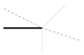
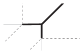
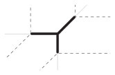
Figure 10. Possible tropicalizations of third-order tangent lines. The intersection of $L$ and $C$ is in bold.

Proof.

According to Proposition 3.11, if $E$ contains a tropical inflection point, then $(C\cap_{\mathbb{T}}L)_{E}\geq 3$. Since $C$ and $L$ are both non-singular, if $E$ does not fulfill the conclusion of the Proposition, then $E$ is one of the following (see Figure 11):

• reduced to a point which is not a common vertex of both $C$ and $L$;

• an unbounded edge of $C$ or $L$ but not of both;

• a bounded segment which is not an edge of $C$ neither of $L$;

• three adjacent edges of $C$ with only one of them being bounded;

The conclusion in the first case follows from Lemmas 3.13 and 3.14. In the last three cases we have

$$(C\cap_{\mathbb{T}}L)_{E}<3.$$

Hence we excluded all cases not listed in the proposition. ∎

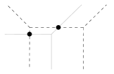
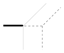
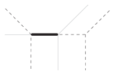
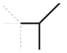
Figure 11. Impossible tropicalizations of third-order tangent lines.

An immediate and important consequence of Proposition 5.1 is that since the vertex of $L$ must be a vertex of $C$, there are only finitely many possibilities for $L$. For each of these possibilities, we use tropical modifications to get a refinement on the possible locations of $p$. If $E$ contains a bounded edge $e$, then we denote by $v_{e}$ the other vertex of $C$ adjacent to $e$. Recall that $l(e)$ is the length of $e$ as an edge of $C$. We define the subset ${\mathfrak{I}}_{L}$ of $E$ as follows :

• if $E=\{v\}$ or $E$ is an unbounded edge of $L$, then ${\mathfrak{I}}_{L}=\{v\}$ (see Figure 12a and 12b);

• if $E$ is a bounded edge $e$ of $C$, then ${\mathfrak{I}}_{L}=\{v,p_{e}\}$ where $p_{e}$ is the point on $e$ at distance $\frac{l(e)}{3}$ from $v$ (see Figure 12c);

• if $E$ is the union of 2 bounded edges $e_{1}$, $e_{2}$, and one unbounded edge $e_{3}$, then

  • if $l(e_{1})>l(e_{2})$, then ${\mathfrak{I}}_{L}=\{p_{e_{1}}\}$ where $p_{e_{1}}$ is the point on $e_{1}$ at distance $\frac{l(e_{1})-l(e_{2})}{3}$ from $v$ (see Figure 12d);

  • if $l(e_{1})=l(e_{2})$, then ${\mathfrak{I}}_{L}$ is the whole edge $e_{3}$ (see Figure 12e);

• if $E$ is the union of 3 bounded edges $e_{1}$, $e_{2}$, and $e_{3}$, then

  • if $l(e_{1})\geq l(e_{2})>l(e_{3})$, then ${\mathfrak{I}}_{L}=\{p_{e_{1}},p_{e_{2}}\}$ where $p_{e_{i}}$ is the point on $e_{i}$ at distance $\frac{l(e_{i})-l(e_{3})}{3}$ from $v$ (see Figure 12f);

  • if $l(e_{1})>l(e_{2})=l(e_{3})$, then ${\mathfrak{I}}_{L}$ is the whole segment $[v;p_{e_{1}}]$ where $p_{e_{1}}$ is the point on $e_{1}$ at distance $\frac{l(e_{1})-l(e_{2})}{3}$ from $v$ (see Figure 12g);

  • if $l(e_{1})=l(e_{2})=l(e_{3})$, then ${\mathfrak{I}}_{L}=\{v\}$ (see Figure 12h).

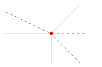
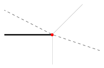
  a)	b)	c)	d)
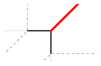
  e)	f)	g)	h)

  Figure 12. Description of ${\mathfrak{I}}_{L}$ in all the possibles cases.

Note that except in two cases, the set ${\mathfrak{I}}_{L}$ is finite.

Proposition 5.2.

The point $p$ is in ${\mathfrak{I}}_{L}$.

Proof.

Without loss of generality, we may assume that $v=(0,0)$ and that $T$ is given by the equation $1+z+w=0$. Let $W$ (resp. $C^{\prime}$) be the tropical modification of ${\mathbb{R}}^{2}$ (resp. $C$) given by the polynomial $1+z+w$. Recall that the tropical hypersurface $W$ has been described in Examples 4.1. We denote $p=(x_{p},y_{p})$. Given a vertex $v_{1}$ of $C$, we denote by $v_{1}^{\prime}$ the vertex of $C^{\prime}$ such that $\pi_{C^{\prime}}(v_{1}^{\prime})=v_{1}$. According to Lemma 4.4, the tropical curve $C^{\prime}$ must have a vertical end $e_{p}$ with $w(e_{p})\geq 3$ such that $\pi_{C^{\prime}}(e_{p})=p$. Let us prove the Proposition case by case.

Case 1: $E=\{v\}$. This case is trivial.

Case 2: $E$ is an unbounded edge $e$ of $C$. We may assume that $E$ is a horizontal edge. Then the proposition follows from Lemma 3.15.

Case 3: $E$ is a bounded edge $e$ of $C$. We may assume that $E$ is a horizontal edge. Since $C^{\prime}\subset W$, we have $v^{\prime}=(0,0,0)$ and $v_{e}^{\prime}=(-l(e),0,0)$ (see Figure 13). If $p=v$ there is nothing to prove, so suppose now that $p\neq v$. We have $(C\cap_{\mathbb{T}}L)_{E}=(C\cap_{\mathbb{T}}L)_{v}+1$. Hence according to Corollary 4.5 and Lemma 3.15, the edge $e_{p}$ has weight exactly 3 and is the only vertical end of $C^{\prime}$ above $e\setminus\{v\}$. According to Corollary 4.7 and the balancing condition, $C^{\prime}$ has exactly 3 edges above $e\setminus\{v\}$: $e_{p}$, an edge with primitive integer direction $(1,0,-1)$ adjacent to $v_{1}^{\prime}$, and an edge with primitive integer direction $(1,0,2)$ adjacent to $v^{\prime}$. Hence, we have $(l(e)+x_{p})+2x_{p}=0$ which reduces to $x_{p}=-\frac{l(e)}{3}$.

\psfrag{V}{$v^{\prime}$}\psfrag{v1}{$v^{\prime}_{1}$}\psfrag{p}{$p$}\psfrag{v2}{$v^{\prime}_{2}$}\psfrag{3}{$3$}\psfrag{ep}{$e_{p}$}\includegraphics[height=142.26378pt,angle={0}]{Case3.eps}

Figure 13. Case 3: $E$ is a bounded edge.

Case 4: $E$ is the union of 2 bounded edges $e_{1}$, $e_{2}$, and one unbounded edge $e_{3}$. We may assume that $e_{1}$ is horizontal, $e_{2}$ is vertical, and that $l(e_{1})\geq l(e_{2})$. Since $C^{\prime}\subset W$, we have

$$v_{e_{1}}^{\prime}=(-l(e_{1}),0,0),\quad v_{e_{2}}^{\prime}=(0,-l(e_{2}),0),\quad\text{and}\quad v^{\prime}=(0,0,-a)\ \text{with}\ a\geq 0.$$

In this case $(C\cap_{\mathbb{T}}L)_{E}=3$. Then, the edge $e_{p}$ has weight exactly 3 and is the only vertical end of $C^{\prime}$ above $E$. Moreover, the curve $C^{\prime}$ is completely determined once $p$ is known.

If $p\in e_{1}$ (i.e. $y_{p}=0$), then the fact that $v^{\prime}$ is a vertex of $C^{\prime}$ gives us the equations $l(e_{2})=a$ and $(l(e_{1})+x_{p})+2x_{p}=a$ which reduces to $x_{p}=-\frac{l(e_{1})-l(e_{2})}{3}$(see Figure 14a).

If $p\in e_{2}$, then $y_{p}=-\frac{l(e_{1})-l(e_{2})}{3}$. Since in this case $y_{p}$ is non-positive, this is possible only if $l(e_{1})=l(e_{2})$ and $y_{p}=0$ (see Figure 14b).

If $p\in e_{3}$, then the vertex $v^{\prime}$ imposes the condition $l(e_{1})=l(e_{2})$. Hence, as soon as $l(e_{1})=l(e_{2})$, the point $p$ may be anywhere on $e_{3}$ (see Figure 14c).

\psfrag{V}{$v^{\prime}$}\psfrag{v1}{$v^{\prime}_{e_{1}}$}\psfrag{p}{$p$}\psfrag{v2}{$v^{\prime}_{e_{2}}$}\psfrag{3}{$3$}\psfrag{ep}{$e_{p}$}\includegraphics[height=156.49014pt,angle={0}]{Case4-1.eps}	\psfrag{V}{$v^{\prime}$}\psfrag{v1}{$v^{\prime}_{e_{1}}$}\psfrag{p}{$p$}\psfrag{v2}{$v^{\prime}_{e_{2}}$}\psfrag{3}{$3$}\psfrag{ep}{$e_{p}$}\includegraphics[height=156.49014pt,angle={0}]{Case4-2.eps}	\psfrag{V}{$v^{\prime}$}\psfrag{v1}{$v^{\prime}_{e_{1}}$}\psfrag{p}{$p$}\psfrag{v2}{$v^{\prime}_{e_{2}}$}\psfrag{3}{$3$}\psfrag{ep}{$e_{p}$}\includegraphics[height=156.49014pt,angle={0}]{Case4-3.eps}
a) $l(e_{1})>l(e_{2})$.	b) $l(e_{1})=l(e_{2})$.	c) $l(e_{1})=l(e_{2})$.

Figure 14. Case 4: $E$ is the union of 3 edges, 2 of them bounded.

Case 5: $E$ is the union of 3 bounded edges $e_{1}$, $e_{2}$, and $e_{3}$. We may assume that $e_{1}$ is horizontal, $e_{2}$ vertical, and that $l(e_{1})\geq l(e_{2})\geq l(e_{3})$. Since $C^{\prime}\subset W$, we have (see Figure 15)

$$v_{e_{1}}^{\prime}=(-l(e_{1}),0,0),\ v_{e_{2}}^{\prime}=(0,-l(e_{2}),0),\ v_{e_{3}}^{\prime}=(l(e_{3}),l(e_{3}),l(e_{3})),\ \ \text{and}\ v^{\prime}=(0,0,-a)\ \text{with}\ a\geq 0.$$

We deduce from $(C\cap_{\mathbb{T}}L)_{E}=4$ that the edge $e_{p}$ may have weight 3 or 4. If $w(e_{p})=4$, then $e_{p}$ is the only vertical end of $C^{\prime}$ above $E$. If $w(e_{p})=3$, there exist exactly two vertical ends of $C^{\prime}$ above $E$, $e_{p}$ and $e^{\prime}$. Note that $w(e^{\prime})=1$, and that we may assume that $w(e_{p})=3$ since the case $w(e_{p})=4$ corresponds to the case $e_{p}=e^{\prime}$. Moreover, the curve $C^{\prime}$ is completely determined once $p$ and $p^{\prime}=\pi_{C^{\prime}}(e^{\prime})=(x^{\prime},y^{\prime})$ are known.

\psfrag{v1}{$v_{e_{1}}^{\prime}$}\psfrag{V2}{$v_{e_{2}}^{\prime}$}\psfrag{V3}{$v_{e_{3}}^{\prime}$}\psfrag{V}{$v^{\prime}$}\psfrag{V5}{$e^{\prime}$}\psfrag{V6}{$e_{p}$}\psfrag{3}{$3$}\psfrag{4}{$4$}\psfrag{=}{$e^{\prime}=e_{p}$}\includegraphics[height=156.49014pt,angle={0}]{Case5-3.eps}	\psfrag{v1}{$v_{e_{1}}^{\prime}$}\psfrag{V2}{$v_{e_{2}}^{\prime}$}\psfrag{V3}{$v_{e_{3}}^{\prime}$}\psfrag{V}{$v^{\prime}$}\psfrag{V5}{$e^{\prime}$}\psfrag{V6}{$e_{p}$}\psfrag{3}{$3$}\psfrag{4}{$4$}\psfrag{=}{$e^{\prime}=e_{p}$}\includegraphics[height=156.49014pt,angle={0}]{Case5-4.eps}
a) If $p,p^{\prime}\in e_{1}$.	b) If $p,p^{\prime}\in e_{3}$.
\psfrag{v1}{$v_{e_{1}}^{\prime}$}\psfrag{V2}{$v_{e_{2}}^{\prime}$}\psfrag{V3}{$v_{e_{3}}^{\prime}$}\psfrag{V}{$v^{\prime}$}\psfrag{V5}{$e^{\prime}$}\psfrag{V6}{$e_{p}$}\psfrag{3}{$3$}\psfrag{4}{$4$}\psfrag{=}{$e^{\prime}=e_{p}$}\includegraphics[height=156.49014pt,angle={0}]{Case5-5.eps}	\psfrag{v1}{$v_{e_{1}}^{\prime}$}\psfrag{V2}{$v_{e_{2}}^{\prime}$}\psfrag{V3}{$v_{e_{3}}^{\prime}$}\psfrag{V}{$v^{\prime}$}\psfrag{V5}{$e^{\prime}$}\psfrag{V6}{$e_{p}$}\psfrag{3}{$3$}\psfrag{4}{$4$}\psfrag{=}{$e^{\prime}=e_{p}$}\includegraphics[height=156.49014pt,angle={0}]{Case5-6.eps}
c) If $p\in e_{1}$ and $p^{\prime}\in e_{2}$.	d) If $p\in e_{2}$ and $p^{\prime}\in e_{1}$.

Figure 15. Case 5: $E$ is the union of 3 bounded edges.

If $p,p^{\prime}\in e_{1}$, then the equations given by the vertex $v^{\prime}$ of $C^{\prime}$ reduce to $l(e_{2})=l(e_{3})=a$ and $x_{p}=-\frac{l(e_{1})-l(e_{2})-x^{\prime}}{3}$. So this is possible only if $l(e_{2})=l(e_{3})$, and in this case the point $p$ may be anywhere on $e_{1}$ as long as it is at distance at most $\frac{l(e_{1})-l(e_{2})}{3}$ from $v$ (See Figure 15a).

In the same way, the points $p$ and $p^{\prime}$ can be both either on $e_{2}$ or on $e_{3}$ if and only if $l(e_{1})=l(e_{3})$, and in this case $p=p^{\prime}=v$. (See Figure 15b).

If $p\in e_{1}$ and $p^{\prime}\in e_{2}$, then we get $x_{p}=-\frac{l(e_{1})-l(e_{3})}{3}$ (See Figure 15c).

If $p\in e_{2}$ and $p^{\prime}\in e_{1}$, then we get $y_{p}=-\frac{l(e_{2})-l(e_{3})}{3}$ (See Figure 15d).

If $p$ is in $e_{3}$, then we get $a=l(e_{1})$ or $a=l(e_{2})$, and $a\leq l(e_{3})+2x_{p}$ which is possible only if $x_{p}=0$.

In the same way, if $p^{\prime}\in e_{3}$, then $p^{\prime}=v$. ∎

5.3. Multiplicities

In the preceding section, we have seen that if $C$ is a non-singular tropical curve in ${\mathbb{R}}^{2}$, then the inflection points of any realization $X$ of $C$ tropicalize in a simple subset $I_{C}$ of $C$, which depends only on $C$. Namely, given a tropical line $L$ whose vertex $v$ is also a vertex of $C$ and such that $v$ is contained in a component of $C\cap L$ of multiplicity at least 3, we define the set ${\mathfrak{I}}_{L}$ as in section 5.2. Then we define $I_{C}=\bigcup{\mathfrak{I}}_{L}$ where $L$ ranges over all such tropical lines. We also define ${\mathfrak{I}}_{C}$ as the set of all connected components of $I_{C}$. In this section we prove that given any element ${\mathcal{E}}$ of ${\mathfrak{I}}_{C}$, the number of inflection points of $X$ which tropicalize in ${\mathcal{E}}$ only depends on ${\mathcal{E}}$.

Let $\Delta\subset{\mathbb{R}}^{2}$ be an integer convex polygon, and let $\delta$ be an edge of $\Delta$. If $\delta$ is not parallel to any edge of $T_{1}$, then we set $r_{\delta}=0$; if $\delta$ is supported on the line with equation $i=a$ (resp. $j=a$, $i+j=a$) and $\Delta$ is contained in the half-plane defined by $i\leq a$ (resp. $j\leq a$, $i+j\geq a$), then we set $r_{\delta}=Card(\delta\cap{\mathbb{Z}}^{2})-1$; otherwise we set $r_{\delta}=2(Card(\delta\cap{\mathbb{Z}}^{2})-1)$; finally, we define

$$i_{\Delta}=3Area(\Delta)-\sum_{\delta\text{ edge of }\Delta}r_{\delta}.$$

Note that $i_{\Delta}<0$ if and only if $\Delta$ is equal to $T_{1}$ or one of its edges.

Definition 5.3.

An element of ${\mathfrak{I}}_{C}$ is called an inflection component of $C$. The multiplicity of an inflection component ${\mathcal{E}}$, denoted by $\mu_{\mathcal{E}}$, is defined as follows

• if ${\mathcal{E}}$ is a vertex of $C$ dual to the primitive triangle $\Delta\neq T_{1}$, then

  $$\mu_{\mathcal{E}}=i_{\Delta};$$

• if ${\mathcal{E}}$ is bounded and contains a vertex of $C$ dual to the primitive triangle $T_{1}$, then

  $$\mu_{\mathcal{E}}=6;$$

• in all other cases,

  $$\mu_{\mathcal{E}}=3.$$

Example 5.4.

We depicted in Figure 16 some honeycomb tropical curves together with their inflection components. Each one of these components is a point of multiplicity 3.

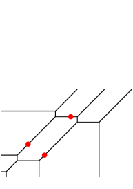
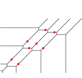
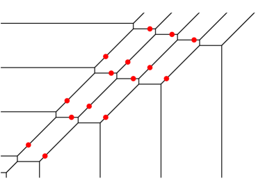
Figure 16. Some honeycomb tropical curves and their inflection points

Proposition 5.5.

For any non-singular tropical curve $C$ in ${\mathbb{R}}^{2}$ with Newton polygon $T_{d}$, we have

$$\sum_{{\mathcal{E}}\in{\mathfrak{I}}_{C}}\mu_{\mathcal{E}}=3d(d-2).$$

Proof.

Let us first introduce some terminology. Let $\Delta$ be a polygon of the dual subdivision of $C$, and let $\delta$ be one of its edges. The edge $\delta$ is said to be bounded if the edge of $C$ dual to $\delta$ is bounded. The edge $\delta$ is said to have $\Delta$-degree 1 if $\delta$ is supported either on the line $\{i=a\}$, or $\{j=a\}$, or $\{i+j=a\}$, and $\Delta$ is contained in the half plane defined respectively by $\{i\geq a\}$, or $\{j\geq a\}$, or $\{i+j\leq a\}$. The number of bounded $\Delta$-degree 1 edges of $\Delta$ is denoted by $\gamma_{\Delta}$. Finally, let $\alpha$ be the number of bounded edges of the dual subdivision of $C$ which are parallel to an edge of $T_{1}$.

From section 5.2 and the definition of $\mu_{\mathcal{E}}$, it follows immediately that for any vertex $v$ of $C$, we have

$$\sum_{{\mathcal{E}}\in{\mathfrak{I}}_{L}}\mu_{\mathcal{E}}=i_{\Delta_{v}}+3\gamma_{\Delta_{v}}$$

where $L$ is the line with vertex $v$. Hence we deduce that

$$\begin{array}[]{lll}\sum_{{\mathcal{E}}\in{\mathfrak{I}}_{C}}\mu_{\mathcal{E}}&=&3Area(T_{d})-2Card(\partial T_{d}\cap{\mathbb{Z}}{{}^{2}})-3\alpha+3\alpha\\ \\ &=&3d(d-2)\end{array}$$

as announced. ∎

To get a genuine correspondence between inflection points of an algebraic curve and the inflection components of its tropicalization, we actually need to pass to projective curves. It is well known that the compactification process we are going to describe now can be adapted to construct general non-singular tropical toric varieties. However, since we will just need to deal with plane projective curves, we restrict ourselves to the construction of tropical projective spaces (see [BJS⁺07]).

As in classical geometry, the tropical projective space ${\mathbb{T}}P^{n}$ of dimension $n\geq 1$ is defined as the quotient of the space ${\mathbb{T}}^{n+1}\setminus\{(-\infty,\ldots,-\infty)\}$ by the equivalence relation

$$v\sim{\text{``}}\lambda v{\text{''}}=v+\lambda(1,\ldots,1).$$

that is

$${\mathbb{T}}P^{n}=({\mathbb{T}}^{n+1}\setminus\{(-\infty,\ldots,-\infty)\})/(1,\ldots,1)$$

Topologically, the space ${\mathbb{T}}P^{n}$ is a simplex of dimension $n$, in particular it is a triangle when $n=2$.

The coordinate system $(x_{1},\ldots,x_{n+1})$ on ${\mathbb{T}}^{n+1}$ induces a tropical homogeneous coordinate system $[x_{1}:\ldots,x_{n+1}]$ on ${\mathbb{T}}P^{n}$, and we have the natural embedding

$$\begin{array}[]{ccc}{\mathbb{R}}^{n}&\longrightarrow&{\mathbb{T}}P^{n}\\ (x_{1},\ldots,x_{n})&\longmapsto&[x_{1}:\ldots,x_{n}:0].\end{array}$$

Hence any tropical variety $V$ in ${\mathbb{R}}^{n}$ has a natural compactification $\overline{V}$ in ${\mathbb{T}}P^{n}$. Also, any non-compact inflection component of a non-singular tropical curve $C$ in ${\mathbb{R}}{{}^{2}}$ compactifies in an inflection component of $\overline{C}$. The map $Val:{\mathbb{K}}^{n+1}\to{\mathbb{T}}^{n+1}$ induces a map $Val:{\mathbb{K}}P^{n}\to{\mathbb{T}}P^{n}$, and if $X$ is an algebraic variety in $({\mathbb{K}}^{*})^{n}$ with closure $\overline{X}$ in ${\mathbb{K}}P^{n}$, we have

$$Trop(\overline{X})=\overline{Trop(X)}.$$

Theorem 5.6.

Let $C$ be a non-singular tropical curve in ${\mathbb{R}}^{2}$ with Newton polygon the triangle $T_{d}$ with $d\geq 2$, and let $X$ be any realization of $C$. Then for any inflection point $p$ of $\overline{X}$, the point $Val(p)$ is contained in an inflection component of $\overline{C}$, and for any inflection component ${\mathcal{E}}$ of $\overline{C}$, exactly $\mu_{\mathcal{E}}$ inflection points of $\overline{X}$ have valuation in ${\mathcal{E}}$.

We postpone the proof of Theorem 5.6 to section 6. The fact that any inflection point of $\overline{X}$ tropicalizes in some inflection component of $C$ has already been proved in Proposition 5.2. The fact that exactly $\mu_{\mathcal{E}}$ inflection points of $\overline{X}$ have valuation in ${\mathcal{E}}$ for any inflection component ${\mathcal{E}}$ follows from Lemmas 6.4, 6.7, 6.8, and 6.9.

5.4. Application to real algebraic geometry

Here we give a real version of Theorem 5.6, which implies immediately Theorem 1. Given ${\mathcal{E}}$ an inflection component of a non-singular tropical curve $C$, we define its real multiplicity $\mu_{\mathcal{E}}^{\mathbb{R}}$ by

$$\mu_{\mathcal{E}}^{\mathbb{R}}=0\ \text{if}\ \mu_{\mathcal{E}}\ \text{is even},\quad\quad\mu_{\mathcal{E}}^{\mathbb{R}}=1\ \text{if}\ \mu_{\mathcal{E}}\ \text{is odd}.$$

Theorem 5.7.

Let $C$ be a non-singular tropical curve in ${\mathbb{R}}^{2}$ with Newton polygon the triangle $T_{d}$ with $d\geq 2$. Suppose that if $v$ is a vertex of $C$ adjacent to 3 bounded edges and such that $\Delta_{v}=T_{1}$, then these edges have 3 different length. Then given any realization $X$ of $C$ over ${\mathbb{R}}{\mathbb{K}}$ and given any inflection component ${\mathcal{E}}$ of $\overline{C}$, exactly $\mu^{\mathbb{R}}_{\mathcal{E}}$ inflection points of $\overline{X}$ have valuation in ${\mathcal{E}}$.

In particular, the curve $\overline{X}$ has exactly $d(d-2)$ inflection points in ${\mathbb{R}}{\mathbb{K}}P{{}^{2}}$, and the curve $\overline{X}(t)$ has also exactly $d(d-2)$ inflection points in ${\mathbb{R}}P{{}^{2}}$ for $t>0$ small enough.

Proof.

Since $\overline{X}$ is defined over ${\mathbb{R}}{\mathbb{K}}$, its inflection points are either in ${\mathbb{R}}{\mathbb{K}}P^{2}$ or they come in pairs of conjugated points. Hence, for each inflection component ${\mathcal{E}}$ of $C$, at least $\mu_{\mathcal{E}}^{\mathbb{R}}$ inflection points of $\overline{X}$ are real and have valuation in ${\mathcal{E}}$.

If $C$ satisfies the hypothesis of the theorem, any of its inflection component ${\mathcal{E}}$ has multiplicity at most 3. Let us prove that the number of inflection points of $C$ of multiplicity $1$ is equal to the number of inflection points of $C$ of multiplicity $2$: this is obviously true when $C$ is a honeycomb tropical curve (i.e. all its edges have direction $(1,0)$, $(0,1)$, or $(1,1)$); one checks easily that if this is true for $C$, then this is also true for any tropical curve whose dual subdivision is obtained from the one of $C$ by a flip; in conclusion this is true for any non-singular tropical curve since any two primitive regular integer triangulations of $T_{d}$ can be obtained one from the other by a finite sequence of flips.

As a consequence, we deduce

$$\begin{array}[]{lll}\sum_{{\mathcal{E}}\in{\mathfrak{I}}_{C}}\mu^{\mathbb{R}}_{\mathcal{E}}&=&\frac{1}{3}\sum_{{\mathcal{E}}\in{\mathfrak{I}}_{C}}\mu_{\mathcal{E}}\\ \\ &=&d(d-2).\end{array}$$

As a consequence the algebraic curve $\overline{X}$ has at least $d(d-2)$ inflection points in ${\mathbb{R}}{\mathbb{K}}P^{2}$. Since $\overline{X}$ is defined over ${\mathbb{R}}{\mathbb{K}}$, it cannot have more according to Theorem 1.1. Hence the curve $\overline{X}$ has exactly $d(d-2)$ inflection points in ${\mathbb{R}}{\mathbb{K}}P^{2}$, and exactly $\mu^{\mathbb{R}}_{\mathcal{E}}$ inflection points of $\overline{X}\cap{\mathbb{R}}{\mathbb{K}}P^{2}$ have valuation in ${\mathcal{E}}$ for any inflection component ${\mathcal{E}}$ of $C$. ∎

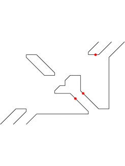
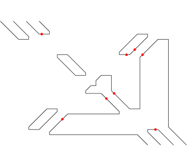
Figure 17. A Harnack curve of degree 3 and 4

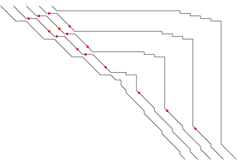
Figure 18. A hyperbolic quintic

Example 5.8.

In Figures 17 and 18, we depicted one possible patchworking of real curve together with its real inflection points for each honeycomb tropical curve depicted in Figure 16.

6. End of the proof of Theorem 5.6

Here we prove that the multiplicity of an inflection component ${\mathcal{E}}$ of $\overline{C}$ corresponds to the number of inflection points of $\overline{X}$ which tropicalizes in ${\mathcal{E}}$. Thanks to tropical modifications, all computations are reduced to elementary local considerations.

Our first task is to study inflection points of algebraic curves in the torus.

6.1. Hessian of a primitive polynomial

Given a polynomial $P(z,w)$ in $k[z,w]$, we define $P^{h}(z,w,u)=z^{2}w^{2}u^{2}P^{hom}(z,w,u)$, and $H_{P}(z,w)=Hess_{P^{h}}(z,w,1)$. Clearly, the curves $V(P)$ and $V(P^{h})$ have the same inflection points in $(k^{*})^{2}$.

Proposition 6.1.

Let $P(z,w)$ be a polynomial in 2 variables over $k$. If the curve $V(P)$ is reduced and does not contain any line, then the number of inflection points of $V(P)$ is at most $i_{\Delta(P)}$ (recall that $i_{\Delta(P)}$ has been defined in section 5.3). Moreover, this number is exactly equal to $i_{\Delta(P)}$ if $k$ is algebraically closed, and $r_{\delta}=0$ and $P^{\delta}$ has no multiple roots in $({\mathbb{C}}^{*})^{2}$ for all edges $\delta$ of $\Delta$.

Proof.

To prove the Proposition, we may suppose that $k$ is algebraically closed. By assumption on $V(P)$, it has finitely many inflection points. The Newton polygon of ${H_{P}}$ is, up to translation, $3\Delta(P)$. Given $\delta$ an edge of $\Delta(P)$, we denote by $\delta_{he}$ the corresponding edge of $\Delta(H_{P})$, by $n_{\delta}$ the number of common roots of the polynomials $P^{\delta}$ and $H_{P}^{\delta_{he}}$, and we define

$$i_{P}=\sum_{\delta\text{ edge of }\Delta(P)}n_{\delta}.$$

Hence, according to Bernstein Theorem, the number of inflection points of $V(P)$ is at most

$$\frac{1}{2}\left(Area(4\Delta(P))-Area(3\Delta(P))-Area(\Delta(P))\right)-i_{P}=3Area(\Delta(P))-i_{P}$$

with equality if $i_{P}=0$.

Hence, we are left to the study of $n_{\delta}$ when $\delta$ ranges over all edges of $\Delta(P)$. Since $P^{h}(z,w,u)$ is divisible by $z^{2}w^{2}u^{2}$, we have $H_{P^{\delta}}=(H_{P})^{\delta_{he}}$ for any edge $\delta$ of $\Delta(P)$. Hence we may suppose that $\Delta(P)$ is reduced to the edge $\delta$. In this case $P^{h}(z,w,u)$ splits into the product of $Card(\delta\cap{\mathbb{Z}}^{2})-1$ binomials, so we may further assume that $Card(\delta\cap{\mathbb{Z}}^{2})=2$. Then the curve $V(P)$ is non-singular in $(k^{*})^{2}$, so the only possibility for $n_{\delta}$ to be equal to 1, is for $V(P)$ to be a line. That is, $\delta$ must be parallel to an edge of $T_{1}$.

In the case when $\Delta(P)$ has an edge $\delta$ supported on the line with equation $i=a$ (resp. $j=a$, $i+j=a$) and $\Delta$ is contained in the half-plane defined by $i\geq a$ (resp. $j\geq a$, $i+j\leq a$), we can refine the upper bound. Without loss of generality, we may assume that $\delta$ is supported on the line with equation $i=0$, and we define $Q(z,w,u)=w^{2}u^{2}P^{hom}(z,w,u)$. The polygon $\Delta(Hess_{Q})$ is contained, up to translation, in the polygon $3\Delta(P)\cap\{i\geq 2\}$, so Bernstein Theorem implies that the number of inflection points of $V(P)$ is at most

$$\frac{1}{2}\left(Area(4\Delta(P)\cap\{i\geq 2\})-Area(3\Delta(P)\cap\{i\geq 2\})-Area(\Delta(P))\right)-\sum_{\delta^{\prime}\neq\delta\text{ edge of }\Delta(Q)}n_{\delta^{\prime}}.$$

Since

$$Area(m\Delta(P)\cap\{i\leq 2\})=Area(\Delta(P)\cap\{i\leq 2\})+4(m-1)(Card(\delta\cap{\mathbb{Z}}^{2})-1),$$

we see that we can in fact substract $2(Card(\delta\cap{\mathbb{Z}}^{2})-1)$ to $3Area(\Delta(P))$ in the upper bound for the number of inflection points of $V(P)$. ∎

Example 6.2.

Any curve over an algebraically closed field, whose Newton polygon is a primitive triangle without any edge parallel to an edge of $T_{1}$, has exactly 3 inflection points in $(k^{*})^{2}$. Indeed, such a curve is non-singular in $(k^{*})^{2}$ and does not contain any line.

Example 6.3.

Proposition 6.1 might not be sharp, even if $k$ is algebraically closed. Indeed, let $X$ be a cubic curve in $kP^{2}$. It is classical (see for example [Sha94]) that a line passing through two inflection points of $X$ also passes through a third inflection point of $X$. Hence, any algebraic curve with Newton polygon the triangle $\Delta$ with vertices $(0,0)$, $(1,2)$, and $(2,1)$, cannot have more than 6 inflection points in $(k^{*})^{2}$, although in this case $i_{\Delta}=7$.

However, Proposition 6.1 is sharp for curves with primitive Newton polygon.

Lemma 6.4.

If $\Delta(P)$ is primitive and distinct from $T_{1}$, then the curve $V(P)$ has exactly $i_{\Delta(P)}$ inflection points in $(k^{*})^{2}$.

Proof.

According to Example 6.2, it remains to check by hand the lemma in the following two particular cases (all coefficients may be chosen equal to 1 since $\Delta(P)$ is primitive):

• $P(z,w)=w+z^{l-1}+z^{l}$ with $l\geq 2$: inflection points are given by the roots in $k^{*}$ of the second derivative of the polynomial $z^{l-1}+z^{l}$. We have 1 (resp. no) such root when $l\geq 3$ (resp. $l=2$).

• $P(z,w)=w+zw+z^{l}$ with $l\geq 0$: inflection points are given by the roots in $k^{*}$ of the second derivative of the function $f(z)=-\frac{z^{l}}{1+z}$. We have 2 (resp. no) such roots when $l\geq 3$ (resp. $l\leq 2$).

∎

Let us fix a polynomial $P(z,w)$ in ${\mathbb{C}}[z,w]\subset{\mathbb{K}}[z,w]$ such that $\Delta(P)$ is primitive and different from $T_{1}$, and define $C=Trop(V(P))$. Recall that both tropical curves $C$ and $Trop(V(H_{P}))$ have the same underlying set. Let $H^{\prime}_{C}$ (resp. $W$) be the tropical modification of $Trop(V(H_{P}))$ (resp. ${\mathbb{R}}^{2}$) given by $P(z,w)$, and $e_{1},e_{2}$, and $e_{3}$ be the three edges of $W$ such that $\pi(e_{i})$ is an edge of $C$. Let $(x_{i},y_{i},z_{i})$ be the primitive integer direction of $e_{i}$ which points to infinity, and by $\widetilde{e}_{i,1},\ldots\widetilde{e}_{i,s_{i}}$ the ends of $H^{\prime}_{C}$ such that $\pi(e_{i,j})=\pi(e_{i})$. Finally we denote by $(x_{i},y_{i},\widetilde{z}_{i,j})$ the primitive integer direction of $\widetilde{e}_{i,j}$ pointing to infinity, and we define

$$z_{H^{\prime}_{C},i}=\sum_{j=1}^{s_{i}}w(\widetilde{e}_{i,j})\widetilde{z}_{i,j}.$$

Lemma 6.5.

The tropical curve $H^{\prime}_{C}$ has a unique vertex, which is also the vertex of $W$. Moreover $H_{C}^{\prime}$ has a vertical end with weight $i_{\Delta(P)}$, and for all $i=1,2,3$ we have

• $z_{H^{\prime}_{C},i}=3z_{i}$ if $(x_{i},y_{i})\neq\pm(1,0),\pm(0,1)$ and $\pm(1,1)$;

• $z_{H^{\prime}_{C},i}=3z_{i}-1$ if $(x_{i},y_{i})=(1,0),(0,1)$ or $(-1,-1)$;

• $z_{H^{\prime}_{C},i}=3z_{i}-2$ if $(x_{i},y_{i})=(-1,0),(0,-1)$ or $(1,1)$.

Proof.

The only thing which does not follow straightforwardly from Proposition 6.1 and Lemma 6.4 is the difference $3z_{i}-z_{H^{\prime}_{C},i}$. However, this difference corresponds exactly to the common roots of the truncation of $P(z,w)$ and $H_{P}(z,w)$ along the corresponding edge of $\Delta(P)$ and $\Delta(H_{P})$, which have been computed in the proof of Proposition 6.1 and Lemma 6.4. ∎

6.2. Localization

In this whole section $C$ is non-singular tropical curve in ${\mathbb{R}}^{2}$ with Newton polygon the triangle $T_{d}$, and $P(z,w)$ is a polynomial of degree $d$ in ${\mathbb{K}}[z,w]$ such that $Trop(V(P))=C$.

The proof of next Lemma is the same as the one of [BB10, Proposition 2.1].

Lemma 6.6.

Let $F$ be a cell of the dual subdivision of $C$. Then the Newton polygon $F^{\prime}$ of $H_{P_{{\mathbb{C}},F}}(z,w)$ is a cell of the dual subdivision of the tropical curve $Trop(V(H_{P}))$, and $(H_{P})_{{\mathbb{C}},F^{\prime}}(z,w)=H_{P_{{\mathbb{C}},F}}(z,w)$.

It follows easily from Lemma 6.6 that the tropical curve $Trop(V(H_{P}))$ has the same underlying set as $C$, and all its edges are of weight 3.

Let $H_{C}^{\prime}$ (resp. $W$) be the tropical modification of $Trop(V(H_{P}))$ (resp. ${\mathbb{R}}^{2}$) given by $z^{2}w^{2}P(z,w)$. It follows from Lemma 6.6 that $H^{\prime}_{C}$ lies entirely in $\pi_{|W}^{-1}(C)$. Following Lemma 4.4, Theorem 5.6 reduces to estimating the weight and the direction of all vertical ends of $H_{C}^{\prime}$.

Lemma 6.7.

Let $v$ be a vertex of $C$ with $\Delta_{v}\neq T_{1}$. Then $H^{\prime}_{C}$ has a vertex $v^{\prime}$ with $\pi(v^{\prime})=v$ and which is also a vertex of $W$. Moreover if $B$ is a ball centered in $v^{\prime}$ of radius $\varepsilon$ small enough, then $B\cap H^{\prime}_{C}$ is equal to a translation of $B^{\prime}\cap H^{\prime}_{C_{v}}$, where $H^{\prime}_{C_{v}}$ is the tropical modification of $Trop(V(H_{P_{{\mathbb{C}},v}}))$ given by $P_{{\mathbb{C}},v}(z,w)$ and $B^{\prime}$ is a ball centered in the origin of radius $\varepsilon$.

Proof.

The tropical curve $H^{\prime}_{C}$ is the tropicalization of the curve in $({\mathbb{K}}^{*})^{3}$ given by the system of equations

(1) $$\left\{\begin{array}[]{l}H_{P}(z,w)=0\\ \\ u-P(z,w)=0\end{array}\right.$$

(the coordinates in $({\mathbb{K}}^{*})^{3}$ are $z,w,$ and $u$). Without loss of generality, we may assume that $v=(0,0)$, that the point $v^{\prime\prime}=(0,0,0)$ is a vertex of $W$, and that the coefficients of the monomials of $P$ corresponding to the vertex of $\Delta_{v}$ have valuation $0$. Hence if $B$ is a small ball centered in $v^{\prime\prime}$, we have that $B\cap H^{\prime}_{C}$ is given by the tropicalization of the curve obtained by plugging $t=0$ in the system (1). According to Lemma 6.6, this tropical curve is exactly the tropical modification of $Trop(V(H_{P_{{\mathbb{C}},v}}))$ given by $P_{{\mathbb{C}},v}(z,w)$. ∎

Lemma 6.7 implies that given $v$ a vertex of $C$ such that $\Delta_{v}\neq T_{1}$, if $B_{v}\subset{\mathbb{R}}^{2}$ is a ball small enough centered in $v$, then the tropical curve $H_{C}^{\prime}$ is completely determined in $B_{v}\times{\mathbb{R}}$ by the tropical modification of $V(H_{P_{{\mathbb{C}},v}})$ given by $P_{{\mathbb{C}},v}(z,w)$. Since this modification is given in Lemma 6.5, we see that the curve $C$ determines the curve $H^{\prime}_{C}$ in $\cup_{v}B_{v}\times{\mathbb{R}}$. Hence it remains to study $H^{\prime}_{C}$ in ${\mathbb{R}}^{3}\setminus(\cup_{v}B_{v}\times{\mathbb{R}})$.

Let $v$ be a vertex of $C$, and $L$ be a tropical line with vertex $v$ and such that $C\cap L$ contains an inflection component of multiplicity at least 3 which is not reduced to $v$. We denote by $E$ the connected component of $C\cap L$ containing $v$. If $\Delta_{v}\neq T_{1}$ we define $E^{\prime}=\overline{E}\setminus\{v\}$, and we define $E^{\prime}=\overline{E}$ otherwise.

Lemma 6.8.

The number of inflection points of $\overline{X}$ with valuation in $E^{\prime}$ is 6 if $E$ is made of 3 bounded edges of $C$, and 3 otherwise.

Proof.

Let $e_{1},\ldots,e_{r}$ (resp. $\widetilde{e}_{1},\ldots,\widetilde{e}_{s}$) be the vertical ends of $H^{\prime}_{C}$ (resp. unbounded edges of $H^{\prime}_{C}$ which are contained in $\pi_{C^{\prime}}^{-1}(E)$ and not vertical), and let $(\widetilde{x}_{i},\widetilde{y}_{i},\widetilde{z}_{i})$ be the primitive integer direction of $\widetilde{e}_{i}$ pointing to infinity. If $s>0$, then there exists a unique unbounded edge $e$ of $E$ such that $\pi_{W}^{-1}(e)$ contains all edges $\widetilde{e}_{1},\ldots,\widetilde{e}_{s}$. Let $(x_{e},y_{e},z_{e})$ be the primitive integer direction pointing to infinity of $e$. The number of inflection points of $\overline{X}$ with valuation in $E^{\prime}$ is equal to

$$\sum_{i=1}^{r}w(e_{i})+3z_{e}-\sum_{i=1}^{s}w(\widetilde{e}_{i})\widetilde{z}_{i}.$$

According to Proposition 5.2, the balancing condition, Lemma 6.5, and Lemma 6.7, this sum is precisely equal to 6 if $E$ is made of 3 bounded edges of $C$, and to 3 otherwise. ∎

So far we have proved Theorem 5.6 in all cases except when $E$ is made of three bounded edges and contains exactly 2 inflection components in its relative interior.

Lemma 6.9.

Suppose that $E$ is made of three bounded edges and contains exactly 2 inflection components $p_{1}$ and $p_{2}$ in its relative interior. Then $\overline{X}$ has exactly 3 inflection points with valuation in $p_{i}$, $i=1,2$.

Proof.

The number of inflection points we are looking for is the weight of the vertical end $e_{i}$ (if any) with $\pi(e_{i})=p_{i}$. According to Proposition 5.2, the balancing condition, Lemma 6.5, and Lemma 6.7, one sees easily that there is no other possibility for this weight other than to be equal to 3. ∎

7. Examples

In this section we use Theorem 5.7 to construct some examples of maximally inflected real curves. In Proposition 7.1 we classify all possible distributions of real inflection points among the connected components of a real quartic. In Proposition 7.2, we construct maximally inflected curves with many connected components and all real inflection points on only one of them.

Before stating Proposition 7.1, let us introduce the following notation: we say that a non-singular real algebraic curve ${\mathbb{R}}X$ in $\mathbb{R}P^{2}$ has inflection type $(n_{1},\ldots,n_{k})$ if ${\mathbb{R}}X$ has exactly $k$ ovals $O_{1},\ldots,O_{k}$ and $O_{i}$ contains exactly $n_{i}$ real inflection points. Note that a maximally inflected real quartic made of two nested ovals automatically has inflection type $(8,0)$.

Proposition 7.1.

The inflection types realized by maximally inflected quartics in $\mathbb{R}P^{2}$ are exactly

$$(8),\ (8,0),\ (6,2),\ (4,4),\ (8,0,0),\ (6,2,0),\ (4,2,2),\ (4,4,0),$$

$$(6,2,0,0),\ (4,2,2,0),\ (4,4,0,0),\ (2,2,2,2).$$

Proof.

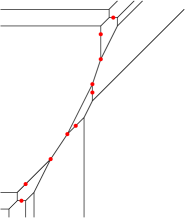
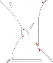
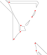
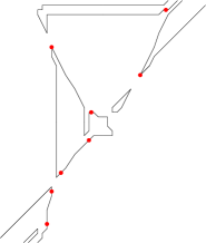
a)	b)	c)	d)

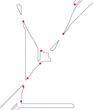
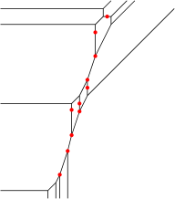
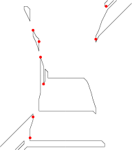
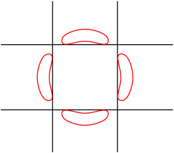
e)	f)	g)	h)

Figure 19. Maximally inflected quartics

The inflection types $(8),(8,0),(6,2),(4,4),(4,2,2)$ and $(2,2,2,2)$ are realized by perturbing the union of two ellipses intersecting in 4 real points. The inflection type $(6,2,2,0)$ is realized by the Harnack quartic constructed in Figure 17. The inflection types $(8,0,0)$, $(6,2,0)$, $(4,4,0)$, and $(4,4,0,0)$ are realized out of the tropical curve depicted in Figure 19a by the patchworkings depicted respectively in Figures 19b,c, d, and e. The inflection type $(4,2,2,0)$ is realized out of the tropical curve depicted in Figure 19f by the patchworking depicted in Figure 19g. Note that some of these inflection types can also be realized by smoothing maximally inflected rational quartics from [KS03].

Hence it remains to prove that the inflection type $(8,0,0,0)$ is not realizable by any quartic. The following argument is due to Kharlamov and simplifies considerably our original proof of this fact. It is a Theorem by Klein ([Kle76b]) that the rigid isotopy class of a non-singular real quartic curve is determined by its isotopy type in ${\mathbb{R}}P^{2}$. Moreover, it is easy to see that this isotopy type also determines the number of real bitangents to the quartic. In the case of real quartics with 4 ovals, one sees by perturbing the union of two conics (see Figure 19h) that all the 28 complex bitangents to these curves are in fact real: 24 bitangents tangent to two distinct ovals, and 4 remaining bitangents. These latter subdivide ${\mathbb{R}}P^{2}$ into 3 quadrangles and 4 triangles, each of these triangles containing exactly one oval of the quartic (see Figure 19h). In particular, no oval has 4 bitangents, which implies that no oval contains 8 real inflection points. ∎

Proposition 7.2.

Given $k\geq 1$, there exists a maximally inflected real algebraic curve of degree $2k$ with one oval containing all real inflection points and $(k-1)^{2}$ other convex ovals, and there exists a maximally inflected real algebraic curve of degree $2k+1$ with the pseudo-line containing all real inflection points and $k^{2}$ other convex ovals.

Proof.

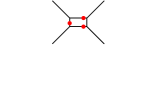
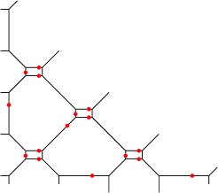
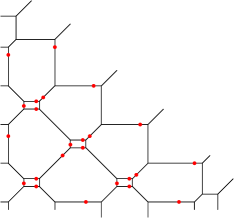
a) Fragment		b) $d=5$		c) $d=6$
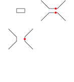
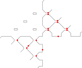
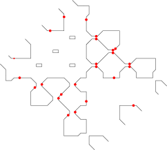
d) Patchworked fragment		e) $d=5$		f) $d=6$

Figure 20. Maximally inflected curves with all inflection points on a single component

Let us consider a non-singular tropical curve of degree $2k+1$ (resp. $2k$) which contains $k^{2}$ (resp. $(k-1)^{2}$) copies of the fragment $\mathcal{F}$ depicted in Figure 20a (see Figure 20b in the case $2k+1=5$, and Figure 20c in the case $2k=6$). The curves whose existence is claim in the proposition can easily be constructed by patchworking all fragments $\mathcal{F}$ as depicted in Figure 20d (see Figure 20e in the case $2k+1=5$, and Figure 20f in the case $2k=6$). ∎

References

- [AN] A. Alessandrini and M. Nessi. On the tropicalization of the Hilbert scheme. arXiv:0912.0082.
- [A] L. Allermann. Tropical intersection products on smooth varieties. arXiv:0904.2693v2.
- [BB10] B. Bertrand and E. Brugallé. On the number of connected component of the parabolic curve. Comptes Rendus de l’Académie des Sciences de Paris, 348(5-6):287–289, 2010.
- [BBM] B. Bertrand, E. Brugallé, and G. Mikhalkin. Genus 0 characteristic numbers of the tropical projective plane. In preparation.
- [BG84] R. Bieri and J. Groves. The geometry of the set of characters induced by valuations. J. Reine Angew. Math., 347:168–195, 1984.
- [BJS+07] T Bogart, A. Jensen, D. Speyer, B. Sturmfels, and R. Thomas. Computing tropical varieties. J. Symbolic Comput., 42(1-2):54–73, 2007.
- [BM] E. Brugallé and G. Mikhalkin. Realizability of superabundant curves. In preparation.
- [BPS08] N. Berline, A. Plagne, and C. Sabbah, editors. Géométrie tropicale. Éditions de l’École Polytechnique, Palaiseau, 2008. available at http://www.math.polytechnique.fr/xups/vol08.html.
-
[Bru09]
E. Brugallé.
Un peu de géométrie tropicale.
Quadrature, (74):10–22, 2009.
available at
http://people.math.jussieu.fr/brugalle/articles/Quadrature/Quadrature.pdf, solutions of the exercises at http://people.math.jussieu.fr/brugalle/articles/Quadrature/CorrectionsQuadrature.pdf. - [IMS07] I. Itenberg, G Mikhalkin, and E. Shustin. Tropical Algebraic Geometry, volume 35 of Oberwolfach Seminars Series. Birkhäuser, 2007.
- [Kap00] M. Kapranov. Amoebas over non-archimedean fields. Preprint, 2000.
- [Kle76a] F Klein. Eine neue Relation zwischen den Singularitäten einer algebraischen Curve. Math. Ann., 10(2), 199–209, 1876.
- [Kle76b] , Klein, F. Über den Verlauf der Abelschen Integrale bei den Kurven vierten Grades. Math. Ann., 10, 365–397, 1876.
- [KS03] Kharlamov, V. and Sottile, F. Maximally inflected real rational curves, Mosc. Math. J., 3(3), 947–987, 1199–1200, 2003.
- [Lop06] Lopez de Medrano, L. Courbure totale des variétés algébriques réelles projectives. Thèse doctorale, 2006, (French).
- [Mik04] G. Mikhalkin. Decomposition into pairs-of-pants for complex algebraic hypersurfaces. Topology, 43:1035–106, 2004.
- [Mik06] G. Mikhalkin. Tropical geometry and its applications. In International Congress of Mathematicians. Vol. II, pages 827–852. Eur. Math. Soc., Zürich, 2006.
- [OP] O. Osserman and S. Payne. Lifting tropical intersections. arXiv:1007.1314.
- [R] Rabinoff, J. Tropical analytic geometry, Newton polygons, and tropical intersections. arXiv:1007.2665.
- [RGST05] J. Richter-Gebert, B. Sturmfels, and T. Theobald. First steps in tropical geometry. In Idempotent mathematics and mathematical physics, volume 377 of Contemp. Math., pages 289–317. Amer. Math. Soc., Providence, RI, 2005.
- [Ri] Risler, J. J. Total curvature of tropical curves. In preparation.
- [Ron98] F. Ronga. Klein’s paper on real flexes vindicated. In W. Pawlucki B. Jakubczyk and J. Stasica, editors, Singularities Symposium - Lojasiewicz 70, volume 44. Banach Center Publications, 1998.
- [Sch04] F. Schuh. An equation of reality for real and imaginary plane curves with higher singularities. Proc. section of sciences of the Royal Academy of Amsterdam, 6:764–773, 1903-1904.
- [Sha94] I. R. Shafarevich. Basic algebraic geometry. 1. Springer-Verlag, Berlin, second edition, 1994.
- [S] K. M. Shaw. A tropical intersection product in matroidal fans. arXiv:1010.3967v1.
- [Vir82] , Viro, O. Ya. Gluing of plane real algebraic curves and constructions of curves of degrees and . Topology (Leningrad, 1982), Lecture Notes in Math., 1060, 187–200, Springer, Berlin,1984.
- [Vir84] Viro, O. Ya. Progress in the topology of real algebraic varieties over the last six years. Russian Math. Surveys, 84(41), 55–82, 1984.
- [Vir88] O. Ya. Viro. Some integral calculus based on Euler characteristic. In Lecture Notes in Math., volume 1346, pages 127–138. Springer Verlag, 1988.
- [Vir01] O. Viro. Dequantization of real algebraic geometry on logarithmic paper. In European Congress of Mathematics, Vol. I (Barcelona, 2000), volume 201 of Progr. Math., pages 135–146. Birkhäuser, Basel, 2001.