The Word Problem in the Baumslag group with a non-elementary Dehn function is polynomial time decidable

Abstract.

We prove that the Word problem in the Baumslag group $G_{(1,2)}={\left\langle a,b~{};~{}a^{a^{b}}=a^{2}\right\rangle}$ which has a non-elementary Dehn function is decidable in polynomial time.

Keywords. Word problem, one-relator groups, Magnus breakdown, power circuits, computational complexity.

2010 Mathematics Subject Classification. 20F10, 11Y16.

1. Introduction

One-relator groups form a very interesting and very mysterious class of groups. In 1910s Dehn proved that the Word problem for the standard presentation of the fundamental group of a closed oriented surface of genus at least two is solvable by what is now called Dehn’s algorithm (see [21] for details). In 1932 Magnus developed a general powerful approach to one-relator groups [19], nowadays known as Magnus break-down procedure (see [20, 18]). In particular, he solved the Word problem (WP) in an arbitrary one-relator group. The decision algorithm is quite complicated and its time complexity is unknown. In fact, we show here that the time function of the Magnus decision algorithm on the Baumslag group

$$G_{(1,2)}={\left\langle a,b\mid b^{-1}a^{-1}bab^{-1}ab=a^{2}\right\rangle}$$

is not bounded by any finite tower of exponents. Furthermore, it is unknown whether there exists any feasible general (uniform) algorithm that solves WP in all one-relator groups, and at present it seems implausible that such algorithm exists. However, it is quite possible that the Word problem in every fixed one-relator group is tractable. In the Magnus collection of open problems in groups theory [5] the following question is posted.

Problem 1.1 ([5], (OR3)).

Is it true that WP in every given one-relator group $G$ is decidable in polynomial time?

The current state of affairs on WP in one-relator groups can be described as follows. On one hand, there are several large classes of one-relator groups where WP is well understood and is decidable in polynomial time (hyperbolic, automatic, linear, etc). On the other hand, there are several sporadic examples of one-relator groups where WP requires a special treatment, though at the end is polynomial time decidable. Finally, there is a few one-relator groups where WP seems especially hard and the time complexity is unknown. These are the most interesting ones in this context.

One of the principal unsolved mysteries on one-relator groups is which of them have a hard WP and why. More precisely, the problem is to determine the “general classes” of one-relator groups and divide the rest (the sporadic, exceptional ones) into some well-defined families.

There are several conjectures that describe large general classes of one-relator groups which we would like to mention here.

1.1. Hyperbolic groups

Notice, that if $G$ is hyperbolic, in particular, if it satisfies the small cancelation condition $C^{\prime}(\frac{1}{6})$, then WP in $G$ is decidable in linear time by Dehn’s algorithm [14]. Since the asymptotic density of the set of words $w\in F(X)$ for which the symmetrized one-relator presentation $\langle X\mid w\rangle$ is $C^{\prime}(\frac{1}{6})$ small cancelation is equal to 1, one may say that for generic one-relator groups the answer to the question above is affirmative. One can check in polynomial (at most quadratic) time if a one-relator presentation, when symmetrized, is $C^{\prime}(\frac{1}{6})$ or not. Hence, it is possible to run in parallel the Magnus break-down process and the Dehn’s algorithm for symmetrized $C^{\prime}(\frac{1}{6})$ presentations and obtain a correct uniform total algorithm that solves WP in one-relator groups, and has Ptime complexity on the set of one-relator groups of asymptotic density 1. Unfortunately, such an algorithm will not be feasible on the most interesting examples of one-relator groups. Some interesting examples of hyperbolic one-relator groups can be found in [15].

Of course, not all one-relator groups are hyperbolic. The famous Baumslag-Solitar one-relator groups

$$B_{(m,n)}={\left\langle a,b\mid b^{-1}a^{m}b=a^{n}\right\rangle},m,n\geq 1,$$

introduced in [6] are not hyperbolic, since the groups $B_{(1,n)}$ are infinite metabelian, and the other ones contain $F_{2}\times\mathbb{Z}$ as a subgroup.

The following outstanding conjecture (see [5]) describes, if true, one-relator hyperbolic groups.

Problem 1.2.

Is every one-relator group without Baumslag-Solitar subgroups hyperbolic?

Independently of the above, it is very interesting to know which one-relator groups contain groups $B_{(m,n)}$.

Problem 1.3.

Is there an algorithm to recognize if a given one-relator group contains a subgroup $B_{(m,n)}$ for some $m,n\geq 1$?

Notice, that in 1968 B. B.  Newman in [24] showed that all one-relator groups with torsion are hyperbolic and, hence, the Word problem for them is decidable in linear time.

1.2. Automatic groups

Automatic groups form another class where WP is easy. It is known that every hyperbolic group is automatic and WP is decidable in at most quadratic time in a given automatic group. Furthermore, the Dehn function in automatic groups is quadratic. We refer to [11] for more details on automatic groups. Observe, that the group $B_{(m,n)}$ is not automatic provided $m\neq n$, since its Dehn function is exponential.

The main challenge in this area is to describe one-relator automatic groups. Answering the following questions would help to understand which one-relator groups are automatic.

Problem 1.4.

Is it true that one-relator groups with a quadratic Dehn function are automatic?

Problem 1.5.

Is it true that one-relator groups with no subgroups isomorphic to $B_{(m,n)},m\neq n$ are automatic?

Problem 1.6 ([5] (OR8)).

Is the one-relator group $\langle X\mid[u,v]\rangle$ automatic for any words $u,v\in F(X)$?

1.3. Linear and residually finite groups

Lipton and Zalstein in [17] proved that WP in linear groups is polynomial time decidable, so one-relator linear groups provide a general subclass of one-relator groups where WP is easy. Until recently, not much was known about linearity of one-relator groups. We refer to [3] for an initial discussion that formed the area for years to come. The real breakthrough came in 2009 when Wise announced in [28] that if a hyperbolic group $G$ has a quasi-convex hierarchy then it is virtually a subgroup of a right angled Artin group and, hence, is linear. This result covers a lot of one-relator groups, in particular all one-relator groups with torsion. There are two interesting cases that we would like to mention here. In [1] Baumslag introduced cyclically pinched one-relator groups as those ones that can be presented as a free product of free groups with cyclic amalgamation

$$\langle X\cup Y\mid u=v\rangle=F(X)\ast_{u=v}F(Y)$$

where $u\in F(X)$ and $v\in F(Y)$ are non-trivial non-primitive elements in the corresponding factors. Similarly, one can define conjugacy pinched one-relator groups as HNN extensions of free groups with cyclic associated subgroups:

$$\langle F(X),t\mid t^{-1}ut=v\rangle$$

Wehrfritz proved in [27] that if non of $u$ and $v$ are proper powers then the group $F(X)\ast_{u=v}F(Y)$ is linear. However, it was shown in [7, 16] that if either $u$ or $v$ is not a proper power then the group $F(X)\ast_{u=v}F(Y)$ is hyperbolic, so WP in these groups is linear time decidable. Similar results hold for conjugacy pinched one-relator groups as well. Observe, that cyclically and conjugacy pinched one-relator hyperbolic groups have quasi-convex hierarchy, so their linearity follows from Wise’s result. On the other hand, WP in hyperbolic groups is easy anyway, so linearity in this case does not give much in terms of the efficiency of WP.

The general problem which one-relator non-hyperbolic groups are linear is wide open. Recall, that every finitely generated linear group is residually finite. Hence, to see that a given one-relator groups is not linear it suffices to show that it is not residually finite.

Notice that there is a special decision algorithm for WP in residually finite finitely presented groups. The algorithm when given such a group $\langle X\mid R\rangle$ and a word $w\in F(X)$ runs two procedures in parallel: the first one enumerates all the consequences of the relators $R$ until the word $w$ occurs, in which case $w=1$ in $G$; while the second one checks if $w$ is non-trivial in some finite quotient of $G$. Since $R$ is finite and $G$ is residually finite, one of the two procedures eventually stops and gives the solution of WP for $w$. However, this algorithm is extremely inefficient. This is why we do not discuss residually finite one-relator groups as a separate class here, but only briefly mention the results that are related to linearity.

Meskin in [22] studied residual finiteness of the following special class of one-relator groups:

$$B(u,v,m,n)={\left\langle X\mid u^{-1}v^{m}u=v^{n}\right\rangle},m,n\geq 1,$$

where $u$ and $v$ are arbitrary non-commuting elements in $F(X)$. He showed that if $m\neq 1,n\neq 1,m\neq n$ then the group $B(u,v,m,n)$ is not residually finite. It follows that the group $B_{(m,n)}$ is residually finite if and only if $m=1$, or $n=1$, or $m=n$.

Later Vol’vachev in [26] found linear representation for all residually finite groups $B(u,v,m,n)$. Sapir and Drutu constructed in [10] the first example of residually finite non-linear one-relator groups. They showed that the group

$$DS=\langle a,t\mid t^{-2}a{t^{2}}=a^{2}\rangle$$

is residually finite and non-linear.

The general classes of one-relator groups described above are the only known ones where WP is polynomial time decidable. Now we describe the known sporadic one-relator groups where WP is presumably hard or requires a special approach.

1.4. Baumslag-Solitar groups

Gersten showed that the groups $B_{(m,n)}$, where $m\neq n$, have exponential Dehn functions [12] (see also [11] and [9]), so they are not hyperbolic or automatic. As we mentioned above the metabelian groups $B_{(1,n)}$ are linear, so WP in them is polynomial time decidable. The non-metabelian groups $B_{(m,n)}$ are not linear, so WP in them requires a special approach. Nevertheless, WP in these groups is polynomial time decidable (see Section 2). It would be interesting to study WP in the groups $B(u,v,m,n)$ which are similar to the Baumslag-Solitar groups.

Problem 1.7.

What is complexity of WP in the groups $B(u,v,m,n)$ ?

1.5. Baumslag group $G_{(1,2)}$

The group $G_{(1,2)}={\left\langle a,b\mid b^{-1}a^{-1}bab^{-1}ab=a^{2}\right\rangle}$ is truly remarkable. Baumslag introduced this group in [2] and showed that all its finite quotients are cyclic. In particular, the group $G_{(1,2)}$ is not residually finite and, hence, is not linear. In [13] Gersten showed that the Dehn function for $G_{(1,2)}$ is not elementary, since it has the lower bound $tower_{2}(\log_{2}(n))$ and later Platonov in [25] proved that $tower_{2}(\log_{2}(n))$ is exactly the Dehn function for $G_{(1,2)}$. This shows that $G_{(1,2)}$ is not hyperbolic, or automatic, or asynchronously automatic. It was conjectured by Gersten that $G_{(1,2)}$ has the highest Dehn function among all one-relator groups. As we have mentioned above the time function for the Magnus break-down algorithm on $G_{(1,2)}$ is not elementary. Taking this into account it was believed until recently that WP in $G_{(1,2)}$ is among the hardest to solve among all one-relator groups. In this paper we show that the Word problem for $G_{(1,2)}$ can be solved in polynomial time. To this end we develop a new technique to compress general exponential polynomials in the base 2 by algebraic circuits (straight-line programs) of a very special type, termed power circuits [23]. We showed that one can do many standard algebraic manipulations (operations $x+y,x-y,x\cdot 2^{y},x\leq y$) over the values of exponential polynomials, whose standard binary length is not bounded by a fixed towers of exponents, in polynomial time if it is kept in the compressed form. This enables us to perform some variations of the standard algorithms in HNN extensions (or similar groups) keeping the actual rewriting in the compressed form. The resulting algorithms are of polynomial time, even though the standard versions are non-elementary.

1.6. Baumslag groups $G_{(m,n)}$

The approach outlined above is quite general and we believe it can be useful elsewhere. In particular, it works for groups of the type $G_{(m,n)}$, where $m$ divides $n$. Here the groups $G_{(m,n)}$ are defined by the following presentations:

$$G_{(m,n)}={\left\langle a,b\mid b^{-1}a^{-1}ba^{m}b^{-1}ab=a^{n}\right\rangle}.$$

Unfortunately, we do not have any compression techniques for the case when $m$ does not divide $n$ and $n$ does not divide $m$. So the following problem seems currently as the main challenge regarding WP in one-relator groups.

Problem 1.8.

What is the time-complexity of the Word problem for $G_{(2,3)}$?

1.7. Generalized Baumslag groups

In [4] Baumslag, Miller and Troeger studied another series of one-relator groups $G(r,w)$ which are similar to the group $G_{(1,2)}$. Namely, if $r,w$ are two non-commuting words in $F(X)$ then put

$$G(r,w)=\langle X\mid r^{r^{w}}=r^{2}\rangle.$$

The group $G(r,w)$ is not residually finite (neither linear nor hyperbolic), it has precisely the same finite quotients as the group $\langle X\mid r\rangle$. These groups surely among the ones with non-easy WP.

Problem 1.9.

Let $r,w$ be two non-commuting elements in $F(X)$.

• What is the Dehn function of $G(r,w)$?

• What is time complexity of WP in $G(r,w)$?

Going a bit further one can consider WP in the following groups

$$G(r,w,m,n)=\langle X\mid(r^{m})^{r^{w}}=r^{n}\rangle.$$

The paper is organized as follows. In section 2 we discuss algorithmic properties of elements of $G_{(1,2)}$ as an HNN extension of the Baumslag-Solitar group, set up the notation, and outline the difficulty of solvig the Word problem using the standard methods for HNN extensions. In Section 3 we define the main tool in our method, namely the power circuits, and present techniques for working with them. In Section 4 we define a representation for words over some alphabet which we call a power sequence. In Section 5 we present the algorithm for solving the Word problem in $G_{(1,2)}$ and prove that its time-complexity is $O(n^{7})$.

2. The group $G_{(1,2)}$

In this section we represent the group $G_{(1,2)}$ as an HNN extension of the Baumslag-Solitar group $B_{(1,2)}$ and describe two rewriting systems ${\mathcal{R}}$ and ${\mathcal{R}}^{\prime}$ to solve WP in $G_{(1,2)}$. The system ${\mathcal{R}}$ represents the classical Magnus breakdown algorithm for $G_{(1,2)}$. To study complexity of rewriting with ${\mathcal{R}}$ we construct an infinite sequence of words $\{w_{k}\}$ such that

• $|w_{k}|\leq 2^{k+2}$;

• it takes at least $tower_{2}(k-1)$ steps for ${\mathcal{R}}$ to rewrite $w_{k}$;

• ${\mathcal{R}}$ rewrites $w_{k}$ into a unique word of length $tower_{2}(k)$.

This shows, in particular, that the time function of the Magnus breakdown algorithm on $G_{(1,2)}$ is not bounded by any finite tower of exponents. Our strategy to solve WP in $G_{(1,2)}$ can be roughly described as follows. We combine many elementary steps in rewriting by ${\mathcal{R}}$ into a single giant step and make it an elementary rewrite of a new system ${\mathcal{R}}^{\prime}$. It is not hard to see that now it takes only polynomially many steps for ${\mathcal{R}}^{\prime}$ to solve WP in $G_{(1,2)}$. In the rest of the paper we show that every elementary rewrite in ${\mathcal{R}}^{\prime}$ (the giant step) can be done in polynomial time in the length of the input, thus proving that WP in $G_{(1,2)}$ is decidable in polynomial time.

2.1. HNN extensions

The purpose of this section is to introduce notation and the technique that we use throughout the paper.

Let $H$ be a group with two isomorphic subgroups $A$ and $B$, and $\varphi:A\rightarrow B$ an isomorphism. Then the group

$$G={\left\langle H,t\mid a^{t}=\varphi(a)\mbox{ for each }a\in A\right\rangle}={\left\langle H,t\mid A^{t}=B\right\rangle}$$

is called the HNN extension of $H$ relative to $\varphi$. We refer to [18] for general facts on HNN extensions. The letter $t$ is called the stable letter. If $H$ is generated by a set $Y$ then $Y\cup\{t\}$ generates $G$ and any word $w$ in the alphabet $(Y\cup\{t\})^{\pm 1}$ can be written in the syllable form:

$$w(H,t)=h_{0}t^{\varepsilon_{1}}h_{1}t^{\varepsilon_{2}}h_{2}\ldots t^{\varepsilon_{n}}h_{n}$$

where $\varepsilon_{i}=\pm 1$ for each $i=1,\ldots,n$ and $h_{i}$ are words in the alphabet $Y^{\pm 1}$. The number $n$ is called the syllable length of $w=w(H,t)$ and denoted by $|w|_{t}$. A pinch in $w$ is a subword of the type $t^{-1}ht$ with $h\in A$ or a subword $tht^{-1}$ where $h\in B$. A word $w$ is reduced if it is freely reduced and contains no pinches.

Theorem (Britton’s lemma, [8]).

Let $G={\left\langle H,t\mid A^{t}=B\right\rangle}$. If a word

$$w(H,t)=h_{0}t^{\varepsilon_{1}}h_{1}t^{\varepsilon_{2}}h_{2}\ldots t^{\varepsilon_{n}}h_{n}$$

represents the trivial element of $G$ then either $n=0$ and $w=_{H}1$ or $w(H,t)$ has a pinch.

Corollary.

Let $G={\left\langle H,t\mid A^{t}=B\right\rangle}$. Assume that

• The Word problem is solvable in $H$.

• The Membership problem is solvable for $A$ and $B$ in $H$.

• The isomorphisms $\varphi$ and $\varphi^{-1}$ are effectively computable.

Then the Word problem in $G$ is solvable.

Proof.

The decision algorithm that easily comes from the Britton’s lemma can be described as rewriting with the following infinite rewriting system ${\mathcal{R}}_{HNN}$:

(1) $$\begin{array}[]{l}\{t^{-1}ht\rightarrow\phi(h)\mid h\in F(Y)\ and\ h\in A\}~{}\cup{}\\ \{tht^{-1}\rightarrow\phi^{-1}(h)\mid h\in F(Y)\ and\ h\in B\}~{}\cup{}\\ \{h\rightarrow\varepsilon\mid h\in F(Y)\ and\ h=_{H}1\}\end{array}$$

where $\varepsilon$ is the empty word.

∎

2.2. The group $G_{(1,2)}$ and Magnus breakdown

Proposition 2.1.

Let $G_{(1,2)}={\left\langle a,b\mid b^{-1}a^{-1}bab^{-1}ab=a^{2}\right\rangle}$. Then the following holds:

• The group $G_{(1,2)}$ is a conjugacy pinched HNN-extension of the Baumslag-Solitar group $B_{(1,2)}={\left\langle a,t\mid t^{-1}at=a^{2}\right\rangle}$ with the stable letter $b$:

  $$G_{(1,2)}={\left\langle B_{(1,2)},b\mid b^{-1}ab=t\right\rangle}$$

• An infinite rewriting system ${\mathcal{R}}$:

  (2) $$\begin{array}[]{l}\{t^{-1}a^{k}t\rightarrow a^{2k}\mid k\in{\mathbb{Z}}\}~{}\cup~{}\{ta^{2k}t^{-1}\rightarrow a^{k}\mid k\in{\mathbb{Z}}\}~{}\cup{}\\ \{b^{-1}a^{k}b\rightarrow t^{k}\mid k\in{\mathbb{Z}}\}~{}\cup~{}\{bt^{k}b^{-1}\rightarrow a^{k}\mid k\in{\mathbb{Z}}\}~{}\cup{}\\ \{aa^{-1}\rightarrow\varepsilon,~{}a^{-1}a\rightarrow\varepsilon,~{}bb^{-1}\rightarrow\varepsilon,~{}b^{-1}b\rightarrow\varepsilon\}\end{array}$$

  is terminating and for any $w=w(a,b)$,

  $$w=_{G}1~{}~{}\Leftrightarrow~{}~{}w\rightarrow_{\mathcal{R}}^{\ast}\varepsilon.$$

  In particular, ${\mathcal{R}}$ gives a decision algorithm for the Word problem in $G_{(1,2)}$,

Proof.

Notice that

$$G_{(1,2)}={\left\langle a,b\mid b^{-1}a^{-1}bab^{-1}ab=a^{2}\right\rangle}={\left\langle a,t,b\mid t^{-1}at=a^{2},~{}b^{-1}ab=t\right\rangle}=$$

$$={\left\langle B_{(1,2)},b\mid b^{-1}ab=t\right\rangle}$$

which proves 1).

To prove 2) observe first that the groups $B_{(1,2)}$ and $G_{(1,2)}$ are HNN extension, which satisfy the properties (G1), (G2), and (G3) from Corollary Corollary. Hence WP in both groups can be solved by the corresponding rewriting systems of the type ${\mathcal{R}}_{HNN}$ from the proof of Corollary Corollary. Combining these rewriting systems into one we obtain the system ${\mathcal{R}}$. It follows that for any $w=w(a,b)$,

$$w=_{G}1~{}~{}\Leftrightarrow~{}~{}w\rightarrow_{\mathcal{R}}^{\ast}\varepsilon.$$

It remains to be seen that ${\mathcal{R}}$ is terminating. To see this associate with each word $w=w(a,b,t)$ a triple $(\alpha,\beta,\gamma)$ where $\alpha$ is a total number of $b$ symbols in $w$, $\beta$ is the total number of $t$ symbols in $w$, and $\gamma=|w|$. It is easy to see that any rewrite from ${\mathcal{R}}$ strictly decreases $(\alpha,\beta,\gamma)$ as an element of ${\mathbb{N}}^{3}$ in the (left) lexicographical order. Now termination of ${\mathcal{R}}$ follows from the fact that ${\mathcal{R}}$ is a well-ordering. ∎

Notice, that the system ${\mathcal{R}}$ is not confluent in general.

Proposition 2.1 states that ${\mathcal{R}}$ solves the Word problem for $G_{(1,2)}$, but it does not give any estimate on the time-complexity of the rewriting procedure. To estimate the complexity of rewriting with ${\mathcal{R}}$ consider a sequence of words over the alphabet of $G_{(1,2)}$ defined as follows

(3) $$\begin{array}[]{ll}w_{0}=&a\\ w_{1}=&(b^{-1}w_{0}b)^{-1}a(b^{-1}w_{0}b)\\ \ldots\\ w_{i+1}=&(b^{-1}w_{i}b)^{-1}a(b^{-1}w_{i}b)\\ \end{array}$$

Lemma 2.2.

Let $G=G_{(1,2)}={\left\langle a,b\mid b^{-1}a^{-1}bab^{-1}ab=a^{2}\right\rangle}$. Then (in the notation above) the following holds:

• for any $i$

  $$w_{i}=_{G}a^{2^{\left.2^{\ldots^{2}}\right\}i~{}times}}=a^{tower_{2}(i)}$$

• $a^{tower_{2}(i)}$ is the only ${\mathcal{R}}$-reduced form of $w_{i}$.

• it takes at least $tower_{2}(i-1)$ elementary rewrites for ${\mathcal{R}}$ to rewrite $w_{i}$ into $a^{tower_{2}(i)}$.

Proof.

By induction on $k$

$$w_{k+1}=(b^{-1}w_{k}b)^{-1}a(b^{-1}w_{k}b)$$

$$=_{G}t^{-2^{\left.2^{\ldots^{2}}\right\}k}}~{}a~{}t^{2^{\left.2^{\ldots^{2}}\right\}k}}=_{G}a^{2^{\left.2^{\ldots^{2}}\right\}k+1}}.$$

which proves 1). Now 2) and 3) are easy. ∎

Theorem 2.3.

The the time function of the Magnus breakdown algorithm on $G_{(1,2)}$ is not bounded by any finite tower of exponents.

Proof.

Since the presentation ${\left\langle a,b\mid b^{-1}a^{-1}bab^{-1}ab=a^{2}\right\rangle}$ for $G_{(1,2)}$ has a unique stable letter $b$ in its relator, the Magnus procedure represents $G_{(1,2)}$ as the HNN extension

$$G_{(1,2)}={\left\langle B_{(1,2)},b\mid b^{-1}ab=t\right\rangle}.$$

Similarly, the presentation ${\left\langle a,t\mid t^{-1}at=a^{2}\right\rangle}$ has a unique stable letter $t$ in its relator, the Magnus procedure represents $B_{(1,2)}$ as the HNN extension of ${\mathbb{Z}}={\left\langle a\right\rangle}$

$$B_{(1,2)}={\left\langle{\left\langle a\right\rangle},t\mid t^{-1}at=a^{2}\right\rangle}.$$

Now, to determine if a given word $w=w(a,b)$ represents the identity of $G_{(1,2)}$ the Magnus process applies the Britton’s lemma to the constructed HNN extensions. The rewriting system ${\mathcal{R}}$ describes precisely the applications of the Britton’s lemma to the word $w$, when one first eliminates all the pinches related to $b$ and then all the pinches related to $t$. Independently of how one realizes the rewriting in Magnus breakdown (rewriting with ${\mathcal{R}}$) in a deterministic fashion the rewriting of the words $w_{i}$ of (3) is essentially unique and takes at least $tower_{2}(i-1)$ elementary rewrites to finish. Notice that the length of the word $w_{i}$ is less than $2^{i+2}-1$ and, as Lemma 2.2 shows, reducing the word $w_{i}$ produces the word of length $tower_{2}(i)$. Hence the result. ∎

2.3. Large scale rewriting in $G_{(1,2)}$

To make the rewriting by ${\mathcal{R}}$ efficient one must be able to:

• work with huge numbers that appear in powers during the computations;

• perform rewrites at bulk, i.e., perform many similar rewrites at once.

In Section 5 we will use the rewriting system

(4) $$\begin{array}[]{rl}{\mathcal{R}}^{\prime}&=\{b^{-1}a^{m}b\rightarrow t^{m},~{}bt^{m}b^{-1}\rightarrow a^{m}\mid m\in{\mathbb{N}}\}\\ &\cup\{t^{k}a^{m}\rightarrow a^{m2^{-k}}t^{-k}\mid m\in{\mathbb{N}},~{}m2^{-k}\in{\mathbb{Z}}\}\\ &\cup\{t^{-k}a^{m}\rightarrow a^{m2^{k}}t^{-k}\mid k\in{\mathbb{N}}\}\\ &\cup\{x^{k}x^{m}\rightarrow t^{k+m}\mid k,m\in{\mathbb{Z}},~{}~{}x\in\{a,b,t\}\}\\ \end{array}$$

instead of the system (2). To perform such rewrites efficiently one must be able to perform the following arithmetic operations:

1. addition and subtraction;

2. multiplication and division by a power of $2$.

In the next section we introduce a representation of integer numbers over which the sequences of operations (O1) and (O2) can be performed efficiently.

3. Power circuits

In this section we define a presentation of integers which we refer to as power circuit presentation and show how one can perform some arithmetic operations over power circuits. See [23] for more details on circuits.

A power circuit is a quadruple $({\mathcal{P}},\mu,M,\nu)$ satisfying the conditions below:

1. ${\mathcal{P}}=(V({\mathcal{P}}),E({\mathcal{P}}))$ a directed graph with no multiple edges and no directed cycles;

2. $\mu:E({\mathcal{P}})\rightarrow\{1,-1\}$ a function called the edge labelling function;

3. $M\subseteq V({\mathcal{P}})$ a set of vertices called the set of marked vertices;

4. and $\nu:M\rightarrow\{-1,1\}$ a function called the sign function.

For an edge $e=v_{1}\rightarrow v_{2}$ in ${\mathcal{P}}$ denote its origin $v_{1}$ by $\alpha(e)$ and its terminus $v_{2}$ by $\beta(e)$. For a vertex $v$ in ${\mathcal{P}}$ define sets

$$In_{v}=\{e\in{\mathcal{P}}\mid\beta(e)=v\}\mbox{ and }Out_{v}=\{e\in{\mathcal{P}}\mid\alpha(e)=v\}.$$

A vertex $v$ in ${\mathcal{P}}$ is called an source if $In_{v}=\emptyset$. Inductively define a function ${\mathcal{E}}:V({\mathcal{P}})\rightarrow\mathbb{R}$ (${\mathcal{E}}$ stands for evaluation) as follows: for $v\in V({\mathcal{P}})$ define

$${\mathcal{E}}(v)=\left\{\begin{array}[]{ll}0&\mbox{if }Out_{v}=\emptyset;\\ 2^{\sum_{e\in Out_{v}}\mu(e){\mathcal{E}}(\beta(e))}&\mbox{otherwise}\\ \end{array}\right.$$

We are interested in presentations of integer numbers only and hence we assume that ${\mathcal{E}}(v)\in{\mathbb{Z}}$ for each $v\in{\mathcal{P}}$. Since ${\mathcal{P}}$ contains no cycles the function ${\mathcal{E}}$ is well-defined. Finally, assign a number ${\mathcal{N}}$ to a defined quadruple $({\mathcal{P}},\mu,M,\nu)$ as follows

$${\mathcal{N}}={\mathcal{N}}({\mathcal{P}},\mu,M,\nu)=\sum_{v\in M}\nu(v){\mathcal{E}}(v).$$

If ${\mathcal{N}}={\mathcal{N}}({\mathcal{P}},\mu,M,\nu)$ then we say that $({\mathcal{P}},\mu,M,\nu)$ is a power circuit presentation of the number ${\mathcal{N}}\in\mathbb{R}$, or that ${\mathcal{N}}$ is represented by $({\mathcal{P}},\mu,M,\nu)$. Throughout the paper we denote the quadruple $({\mathcal{P}},\mu,M,\nu)$ simply by ${\mathcal{P}}$.

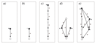
Figure 1. Power circuits representing integers $1$, $-1$, $16$, $2$ and $35$. Black vertices denote the marked vertices. An edge $e$ is labeled with $+$ if $\mu(e)=1$, a marked vertex $v$ is labeled with $+$ if $\nu(v)=1$.

For a circuit ${\mathcal{P}}$ denote by $|{\mathcal{P}}|$ the number $|V({\mathcal{P}})|+|E({\mathcal{P}})|$ called the size of the circuit and by ${\mathcal{N}}({\mathcal{P}})$ the integer represented by ${\mathcal{P}}$.

3.1. Zero vertices in power circuits

A vertex $z$ in ${\mathcal{P}}$ is called zero if $Out_{z}=\emptyset$. It follows from the definition of the function ${\mathcal{E}}$ that $z$ is a zero vertex in ${\mathcal{P}}$ if and only if ${\mathcal{E}}(z)=0$. Clearly, each non-trivial circuit has at least zero vertex. If ${\mathcal{P}}$ has more than one zero vertex then its size can be reduced.

Lemma 3.1 ([23]).

Let $z_{1}$ and $z_{2}$ be distinct zero vertices of a circuit ${\mathcal{P}}$ and ${\mathcal{P}}^{\prime}$ a circuit obtained from ${\mathcal{P}}$ by gluing $z_{1}$ and $z_{2}$ together. Then $|V({\mathcal{P}})|=|V({\mathcal{P}}^{\prime})|+1$ and ${\mathcal{N}}({\mathcal{P}})={\mathcal{N}}({\mathcal{P}}^{\prime})$.

3.2. Addition and subtraction

Let ${\mathcal{P}}_{1}$ and ${\mathcal{P}}_{2}$ be two circuits. To compute a circuit ${\mathcal{P}}_{+}$ such that ${\mathcal{N}}({\mathcal{P}}_{+})={\mathcal{N}}({\mathcal{P}}_{1})+{\mathcal{N}}({\mathcal{P}}_{2})$ one can take a union of ${\mathcal{P}}_{1}$ and ${\mathcal{P}}_{2}$ leaving the labeling functions the same. Clearly the obtained result satisfies the equality ${\mathcal{N}}({\mathcal{P}}_{+})={\mathcal{N}}({\mathcal{P}}_{1})+{\mathcal{N}}({\mathcal{P}}_{2})$. Similarly, to compute a circuit ${\mathcal{P}}_{-}$ such that ${\mathcal{N}}({\mathcal{P}}_{-})={\mathcal{N}}({\mathcal{P}}_{1})-{\mathcal{N}}({\mathcal{P}}_{2})$ one can take a union of ${\mathcal{P}}_{1}$ and ${\mathcal{P}}_{2}$ leaving the labeling functions on ${\mathcal{P}}_{1}$ the same and changing the labeling function on $M({\mathcal{P}}_{2})$ to the opposite. Clearly the obtained result satisfies the required equality. See Figure 2 for an example of difference of two circuits.

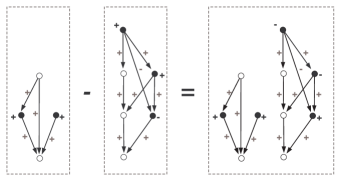
Figure 2. Taking difference of circuits d) and e) from Figure 1.

Proposition 3.2 ([23]).

Let ${\mathcal{P}}_{1}$ and ${\mathcal{P}}_{2}$ be power circuits and ${\mathcal{P}}_{+}={\mathcal{P}}_{1}+{\mathcal{P}}_{2}$. Then ${\mathcal{N}}({\mathcal{P}}_{+})={\mathcal{N}}({\mathcal{P}}_{1})+{\mathcal{N}}({\mathcal{P}}_{2})$, $|V({\mathcal{P}}_{+})|=|V({\mathcal{P}}_{1})|+|V({\mathcal{P}}_{2})|$, and $|E({\mathcal{P}}_{+})|=|E({\mathcal{P}}_{1})|+|E({\mathcal{P}}_{2})|$. Moreover, ${\mathcal{P}}_{+}$ and ${\mathcal{P}}_{-}$ are computed in time $O(|{\mathcal{P}}_{1}|+|{\mathcal{P}}_{2}|)$.

3.3. Comparison (circuit reduction)

In this section we shortly describe the procedure called the reduction of power circuits. For the precise definition of a reduced circuit see [23]. The main property of reduced circuits is that ${\mathcal{E}}(v_{1})={\mathcal{E}}(v_{2})$ if and only if $v_{1}=v_{2}$.

Theorem 3.3 ([23]).

There exists an algorithm which for every power circuit ${\mathcal{P}}$ constructs an equivalent reduced circuit ${\mathcal{P}}^{\prime}$ such that

$$|V({\mathcal{P}}^{\prime})|\leq|V({\mathcal{P}})|+1\mbox{ and }|M({\mathcal{P}}^{\prime})|\leq|M({\mathcal{P}})|,$$

and orders vertices of ${\mathcal{P}}^{\prime}$ according to their ${\mathcal{E}}$ values. Moreover, the time complexity of the procedure is $O(|V({\mathcal{P}})|^{3})$.

Proposition 3.4 ([23]).

Let ${\mathcal{P}}$ be a reduced circuit. Then ${\mathcal{N}}({\mathcal{P}})=0$ if and only if ${\mathcal{P}}$ has no marked vertices. If ${\mathcal{P}}$ is not trivial and if $v$ is the vertex with maximal ${\mathcal{E}}$ value then ${\mathcal{N}}({\mathcal{P}})>0$ if and only if $\nu(v)=1$.

Proposition 3.5 ([23]).

There exists a deterministic algorithm which for every power circuit ${\mathcal{P}}$ computes

$$Sign({\mathcal{P}})=\left\{\begin{array}[]{ll}-1,&\mbox{if }{\mathcal{N}}({\mathcal{P}})<0;\\ 0,&\mbox{if }{\mathcal{N}}({\mathcal{P}})=0;\\ 1,&\mbox{if }{\mathcal{N}}({\mathcal{P}})>0.\\ \end{array}\right.$$

Moreover, the time complexity of that procedure is bounded above by $O(|V({\mathcal{P}})|^{3})$.

Proposition 3.6 ([23]).

Let ${\mathcal{P}}$ be a reduced power circuit, $\{v_{1},\ldots,v_{n}\}$ a set of all its vertices ordered according to their ${\mathcal{E}}$ values, and $i=\min\{j\mid v_{j}\in M\}$. Then ${\mathcal{N}}({\mathcal{P}})$ is divisible by $2^{M}$ if and only if ${\mathcal{E}}(v_{i})$ is.

3.4. Multiplication and division by a power of two

Let ${\mathcal{P}}_{1}$ and ${\mathcal{P}}_{2}$ be power circuits. Assume that ${\mathcal{N}}({\mathcal{P}}_{2})>0$. In this section we outline a procedure for constructing circuits ${\mathcal{P}}_{\bullet}$ and ${\mathcal{P}}_{\circ}$ satisfying

$${\mathcal{N}}({\mathcal{P}}_{\bullet})={\mathcal{N}}({\mathcal{P}}_{1})\bullet{\mathcal{N}}({\mathcal{P}}_{2}):={\mathcal{N}}({\mathcal{P}}_{1})\cdot 2^{{\mathcal{N}}({\mathcal{P}}_{2})}$$

and

$${\mathcal{N}}({\mathcal{P}}_{\circ})={\mathcal{N}}({\mathcal{P}}_{1})\circ{\mathcal{N}}({\mathcal{P}}_{2}):=\frac{{\mathcal{N}}({\mathcal{P}}_{1})}{2^{{\mathcal{N}}({\mathcal{P}}_{2})}}.$$

Recall that ${\mathcal{N}}({\mathcal{P}}_{1})=\sum_{v\in M_{1}}\nu(v){\mathcal{E}}(v)$, where ${\mathcal{E}}(v)=2^{\sum_{e\in Out_{v}}\mu(e){\mathcal{E}}(\beta(e))}$ is a power of $2$. Hence, to multiply ${\mathcal{N}}({\mathcal{P}}_{1})$ by $2^{{\mathcal{N}}({\mathcal{P}}_{2})}$ one can multiply the values of ${\mathcal{E}}(v)$ by $2^{{\mathcal{N}}({\mathcal{P}}_{2})}$ for each $v\in M({\mathcal{P}}_{1})$ which corresponds to increase of the value of the sum $\sum_{e\in Out_{v}}\mu(e){\mathcal{E}}(\beta(e))$ by ${\mathcal{N}}({\mathcal{P}}_{2})$. Thus, to multiply ${\mathcal{N}}({\mathcal{P}}_{1})$ by $2^{{\mathcal{N}}({\mathcal{P}}_{2})}$ one can perform the following steps:

1. make each marked vertex $v$ in ${\mathcal{P}}_{1}$ a source;

2. take a union of ${\mathcal{P}}_{1}$ and ${\mathcal{P}}_{2}$;

3. for each $v_{1}\in M_{1}$ and $v_{2}\in M_{2}$ add an edge $e=v_{1}\rightarrow v_{2}$ and put $\mu(e)=\nu(v_{2})$;

4. unmark marked vertices of ${\mathcal{P}}_{2}$.

See Figure 3 for an example.

In this paper we work with integer numbers only. Hence the operation $\circ$ is not always defined for all pairs ${\mathcal{P}}_{1}$, ${\mathcal{P}}_{2}$ of circuits. To check if ${\mathcal{P}}_{1}\circ{\mathcal{P}}_{2}$ is defined one can reduce the presentation of ${\mathcal{P}}_{1}$ and check the conditions of Proposition 3.6. To actually multiply ${\mathcal{P}}_{1}$ by $2^{-{\mathcal{N}}({\mathcal{P}}_{2})}$ one needs to 1) reduce ${\mathcal{P}}_{1}$, 2) invert the value of ${\mathcal{P}}_{2}$ and, 3) apply the algorithm outlined above to compute ${\mathcal{P}}_{\circ}$.

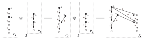
Figure 3. Multiplication by a power of $2$.

Proposition 3.7.

Let ${\mathcal{P}}_{1}$ and ${\mathcal{P}}_{2}$ be power circuits and, ${\mathcal{P}}_{\bullet}$ and ${\mathcal{P}}_{\circ}$ are obtained by the outlined above procedures. Then

• ${\mathcal{N}}({\mathcal{P}}_{\bullet})={\mathcal{N}}({\mathcal{P}}_{1})2^{{\mathcal{N}}({\mathcal{P}}_{2})}$ and ${\mathcal{N}}({\mathcal{P}}_{\circ})=\frac{{\mathcal{N}}({\mathcal{P}}_{1})}{2^{{\mathcal{N}}({\mathcal{P}}_{2})}}$;

• $|V({\mathcal{P}}_{\bullet})|,|V({\mathcal{P}}_{\circ})|\leq|V({\mathcal{P}}_{1})|+|V({\mathcal{P}}_{2})|+|M_{1}|$.

• The time required to construct ${\mathcal{P}}_{\bullet}$ is bounded by $O(|{\mathcal{P}}_{1}|+|{\mathcal{P}}_{2}|)$.

• The time required to construct ${\mathcal{P}}_{\circ}$ is bounded by $O(|V({\mathcal{P}}_{1})|^{3}+|{\mathcal{P}}_{2}|+|M_{1}|\cdot|M_{2}|)$.

Proof.

Straightforward to check. ∎

4. Power sequences

Let $X$ be a group alphabet, $x_{1},\ldots,x_{n}\in X^{\pm 1}$, ${\mathcal{P}}_{1},\ldots,{\mathcal{P}}_{n}$ power circuits. A sequence ${\mathcal{S}}=(x_{1},{\mathcal{P}}_{1}),\ldots,(x_{n},{\mathcal{P}}_{n})$ is called a power sequence. We say that a power sequence ${\mathcal{S}}$ represents a word

$$W({\mathcal{S}})=x_{1}^{{\mathcal{N}}({\mathcal{P}}_{1})}\ldots x_{n}^{{\mathcal{N}}({\mathcal{P}}_{n})}.$$

The following characteristics of power sequences are used in our analysis in Section 5. We denote by $M({\mathcal{S}})$ the total number of marked vertices in its circuits, i.e.,

$$M({\mathcal{S}})=\sum_{(x,{\mathcal{P}})\in{\mathcal{S}}}|M({\mathcal{P}})|,$$

and $V({\mathcal{S}})$ the total number of vertices in its circuits, i.e.,

$$V({\mathcal{S}})=\sum_{(x,{\mathcal{P}})\in{\mathcal{S}}}|V({\mathcal{P}})|.$$

If ${\mathcal{S}}$ represents a word $w=x_{1}^{p_{1}}\ldots x_{n}^{p_{n}}$ and $g=x_{i}^{p_{i}}\ldots x_{j}^{p_{j}}$ is a subword of $w$ denote by ${\mathcal{S}}_{g}$ the segment of ${\mathcal{S}}$ corresponding to $g$.

A power sequence is reduced if it does not contain

1. a pair $(x,{\mathcal{P}})$ where ${\mathcal{N}}({\mathcal{P}})=0$,

2. a subsequence $(x,{\mathcal{P}}),(x,{\mathcal{P}}^{\prime})$.

To reduce a power sequence ${\mathcal{S}}$ one can consequently replace non-reduced subsequences $(x,{\mathcal{P}}),(x,{\mathcal{P}}^{\prime})$ by the corresponding pairs $(x,{\mathcal{P}}+{\mathcal{P}}^{\prime})$, and remove the pairs (R1). The described process is called a reduction of a power sequence.

Proposition 4.1.

Let ${\mathcal{S}}$ be a power sequence and ${\mathcal{S}}^{\prime}$ be obtained by reducing ${\mathcal{S}}$. Then ${\mathcal{S}}$ and ${\mathcal{S}}^{\prime}$ represents the same element of the corresponding free group $F(A)$. Furthermore, $M({\mathcal{S}}^{\prime})\leq M({\mathcal{S}})$ and $V({\mathcal{S}}^{\prime})\leq V({\mathcal{S}})$. The time complexity of reduction is not greater than $O(|V({\mathcal{S}})|^{3})$.

Proof.

Follows from Proposition 3.2.

∎

5. Algorithm for the Word problem in $G_{(1,2)}$

In this section we describe an algorithm for the Word problem in $G_{(1,2)}$ and prove that it has polynomial time complexity. All words in this section are processed in power sequences. More details are given in Section 5.1. In Section 5.2 we give the final complexity estimate.

Word problem for $G_{(1,2)}$

0:  A word $w=w(a,b,t)$.

0:  $Yes$ if $w$ represents the identity in $G_{(1,2)}$, $No$ otherwise.

1:  Represent $w$ as a product of powers

(5) $$w(a,b,t)=g_{0}(a,t)b^{\varepsilon_{1}}g_{1}(a,t)b^{\varepsilon_{2}}g_{2}(a,t)\ldots b^{\varepsilon_{n}}g_{n}(a,t)$$

where

(6) $$g_{i}(a,t)=a^{m_{i,0}}t^{\delta_{i,1}}a^{m_{i,1}}t^{\delta_{i,2}}a^{m_{i,2}}\ldots t^{\delta_{i,k_{i}}}a^{m_{i,k_{i}}}$$

and $\varepsilon_{i},\delta_{i,j},m_{i,j}\in{\mathbb{Z}}$.

2:  Compute a power sequence ${\mathcal{S}}$ representing $w$.

3:  while ${\mathcal{S}}$ contains a subsequence ${\mathcal{S}}_{g_{i}}$ satisfying the follwoing do

4:        if $\varepsilon_{i}<0$, $\varepsilon_{i+1}>0$, and ${\mathcal{S}}_{g_{i}}=_{B}a^{p}$ for some $p\in{\mathbb{Z}}$ then

5:               Replace a subsequence $(b,\varepsilon_{i}){\mathcal{S}}_{g_{i}}(b,\varepsilon_{i+1})$ in ${\mathcal{S}}$ with $(b,\varepsilon_{i}+1),(t,p),(b,\varepsilon_{i+1}-1)$.

6:        end if

7:        if $\varepsilon_{i}>0$, $\varepsilon_{i+1}<0$, and ${\mathcal{S}}_{g_{i}}=_{B}t^{p}$ for some $p\in{\mathbb{Z}}$ then

8:               Replace a subsequence $(b,\varepsilon_{i}){\mathcal{S}}_{g_{i}}(b,\varepsilon_{i+1})$ in ${\mathcal{S}}$ with $(b,\varepsilon_{i}+1),(a,p),(b,\varepsilon_{i+1}-1)$.

9:        end if

10:  end while

11:  if The obtained ${\mathcal{S}}$ involves letter $b$ then

12:        return  $No$.

13:  end if

14:  if If the obtained sequence represents the trivial element in $B_{(1,2)}$ then

15:        return  $Yes$.

16:  else

17:        return  $No$.

18:  end if

A single transformation on line 5 and line 8 decreases the total power of $b$ in a power sequence ${\mathcal{S}}$ by $2$. Hence Algorithm 5 performs at most $|w|/2$ transformations. Now, it remains to describe a procedure for checking if ${\mathcal{S}}_{g_{i}}=_{G}a^{p}$ or ${\mathcal{S}}_{g_{i}}=_{G}t^{p}$ for some $p\in{\mathbb{Z}}$ for some $p\in{\mathbb{Z}}$. This is done in Section 5.1.

5.1. Word processing in $B_{(1,2)}$

Let

(7) $$(a,{\mathcal{P}}_{m_{0}}),(t,{\mathcal{P}}_{\delta_{1}}),(a,{\mathcal{P}}_{m_{1}}),(t,{\mathcal{P}}_{\delta_{2}}),(a,{\mathcal{P}}_{m_{2}})\ldots(t,{\mathcal{P}}_{\delta_{k}}),(a,{\mathcal{P}}_{m_{k}})$$

be a power sequence representing a word

$$g=a^{m_{0}}t^{\delta_{1}}a^{m_{1}}t^{\delta_{2}}a^{m_{2}}\ldots t^{\delta_{k}}a^{m_{k}}$$

over the alphabet of $B_{(1,2)}$.

Proposition 5.1 (All non-positive powers).

Consider a sequence (7). Assume that $\delta_{1}+\ldots+\delta_{i}\leq 0$ for every $i=1,\ldots,k$. Then $g=a^{M}t^{\sigma}$ in $G_{(1,2)}$ where

$$\sigma=\sum_{i=1}^{k}\delta_{i}\mbox{ and }M=\sum_{i=0}^{k}m_{i}\cdot 2^{\sum_{j=1}^{i}\delta_{j}}.$$

Furthermore, there exist power circuits ${\mathcal{P}}_{M}$ and ${\mathcal{P}}_{\sigma}$ such that ${\mathcal{N}}({\mathcal{P}}_{M})=M$ and ${\mathcal{N}}({\mathcal{P}}_{\sigma})=\sigma$ and

1. $|V({\mathcal{P}}_{\sigma})|=\sum_{j=1}^{k}|V({\mathcal{P}}_{\delta_{j}})|$ and $|V({\mathcal{P}}_{M})|\leq\sum_{j=0}^{k}(|V({\mathcal{P}}_{m_{j}})|+|M({\mathcal{P}}_{m_{j}})|)+\sum_{j=1}^{k}|V({\mathcal{P}}_{\delta_{j}})|$;

2. $|M({\mathcal{P}}_{\sigma})|=\sum_{j=1}^{k}|M({\mathcal{P}}_{\delta_{j}})|$ and $|M({\mathcal{P}}_{M})|=\sum_{j=0}^{k}|M({\mathcal{P}}_{m_{j}})|.$

Proof.

The equality $g=a^{M}t^{\sigma}$ in $G_{(1,2)}$ is obvious. A circuit ${\mathcal{P}}_{\sigma}$ can be constructed by laying down circuits for ${\mathcal{P}}_{\delta_{1}},\ldots,{\mathcal{P}}_{\delta_{k}}$. A circuit ${\mathcal{P}}_{M}$ is obtained by

• laying down the circuits ${\mathcal{P}}_{m_{0}},\ldots,{\mathcal{P}}_{m_{k}}$, ${\mathcal{P}}_{\delta_{1}},\ldots,{\mathcal{P}}_{\delta_{k}}$;

• adding edges between ${\mathcal{P}}_{m_{i}}$ and ${\mathcal{P}}_{\delta_{j}}$ as it is done in multiplication by a power of two (see Section 3.4);

• removing marked vertices from ${\mathcal{P}}_{\delta_{j}}$’s.

See Figure 4.

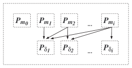
Figure 4. Scheme for a circuit representing $\sum_{i=0}^{k}{\mathcal{P}}_{m_{i}}\circ{\left(\sum_{j=1}^{i}{\mathcal{P}}_{\delta_{j}}\right)}$.

Clearly ${\mathcal{P}}_{M}$ and ${\mathcal{P}}_{\sigma}$ satisfy properties (1) and (2). ∎

We call the transformation of Proposition 5.1 a (T1)-transformation. Applying (T1)-transformations to subsequences of (7) we either obtain a power sequence

(8) $$(a,{\mathcal{P}}_{M_{0}}),(t,{\mathcal{P}}_{\sigma_{1}}),(a,{\mathcal{P}}_{M_{1}}),\ldots,(a,{\mathcal{P}}_{M_{n-1}}),(t,{\mathcal{P}}_{\sigma_{n}}),(a,{\mathcal{P}}_{M_{n}}),\phantom{,(t,{\mathcal{P}}_{\sigma_{n+1}})}$$

where $\sigma_{i}>0$ for every $i=1,\ldots,n$; or a power sequence

(9) $$(a,{\mathcal{P}}_{M_{0}}),(t,{\mathcal{P}}_{\sigma_{1}}),(a,{\mathcal{P}}_{M_{1}}),\ldots,(a,{\mathcal{P}}_{M_{n-1}}),(t,{\mathcal{P}}_{\sigma_{n}}),(a,{\mathcal{P}}_{M_{n}}),(t,{\mathcal{P}}_{\sigma_{n+1}}),$$

where $\sigma_{i}>0$ for every $i=1,\ldots,n$ and $\sigma_{n+1}<0$. Furthermore, for (8) there exist a sequence $1\leq l_{0}<l_{1}<\ldots<l_{n}=k$ such that

(10) $${\mathcal{P}}_{\sigma_{i}}={\mathcal{P}}_{\delta_{l_{i}}}+\ldots+{\mathcal{P}}_{\delta_{l_{i+1}-1}}\mbox{ and }{\mathcal{P}}_{M_{i}}=\sum_{i=l_{i}-1}^{l_{i+1}-1}{\mathcal{P}}_{m_{i}}\circ{\left(\sum_{j=l_{i}}^{i}{\mathcal{P}}_{\delta_{j}}\right)}.$$

Similar formulas hold for (9). The next lemma follows from the Britton’s lemma.

Lemma 5.2.

If a sequence (8) or (9) represents in $B_{(1,2)}$ an element $a^{p}$ or $t^{p}$ for some $p\in{\mathbb{Z}}$ then for every $i=1,\ldots,n$ the condition

$$2^{-\sigma_{i}}{\left(\ldots+2^{-\sigma_{n-2}}{\left(M_{n-2}+2^{-\sigma_{n-1}}{\left(M_{n-1}+2^{-\sigma_{n}}M_{n}\right)}\right)}\right)}\in{\mathbb{Z}}$$

is satisfied.

Proposition 5.3 (All positive powers).

Consider a sequence (8) or (9) representing an element $g$ in $B_{(1,2)}$. If for every $i=1,\ldots,n$ the condition

$$2^{-\sigma_{i}}{\left(\ldots+2^{-\sigma_{n-2}}{\left(M_{n-2}+2^{-\sigma_{n-1}}{\left(M_{n-1}+2^{-\sigma_{n}}M_{n}\right)}\right)}\right)}\in{\mathbb{Z}}$$

is satisfied then $g=a^{M}t^{\sigma}$, where $\sigma=\sum_{i=0}^{n}\sigma_{i}$ and

$$M={\left(M_{0}+\ldots{\left(M_{n-2}+{\left(M_{n-1}+M_{n}\circ\sigma_{n}\right)}\circ\sigma_{n-1}\right)}\ldots\circ\sigma_{1}\right)}.$$

Furthermore, there exist power circuits ${\mathcal{P}}_{M}$ and ${\mathcal{P}}_{\sigma}$ such that ${\mathcal{N}}({\mathcal{P}}_{M})=M$ and ${\mathcal{N}}({\mathcal{P}}_{\sigma})=\sigma$ satisfying

1. $|V({\mathcal{P}}_{\sigma})|=\sum_{j=1}^{n}|V({\mathcal{P}}_{\sigma_{j}})|$ and $|V({\mathcal{P}}_{M})|\leq\sum_{j=0}^{n}(|V({\mathcal{P}}_{M_{j}})|+|M({\mathcal{P}}_{M_{j}})|)+\sum_{j=1}^{n}|V({\mathcal{P}}_{\sigma_{j}})|$;

2. $|M({\mathcal{P}}_{\sigma})|=\sum_{j=1}^{n}|M({\mathcal{P}}_{\sigma_{j}})|$ and $|M({\mathcal{P}}_{M})|=\sum_{j=0}^{k}|M({\mathcal{P}}_{M_{j}})|.$

Proof.

The equality $g=a^{M}t^{\sigma}$ follows from the Britton’s lemma. To construct a circuit ${\mathcal{P}}_{\sigma}$ we lay down circuits for ${\mathcal{P}}_{\sigma_{1}},\ldots,{\mathcal{P}}_{\sigma_{n}}$. Clearly, ${\mathcal{P}}_{\sigma}$ satisfies the properties (1) and (2).

We construct a circuit ${\mathcal{P}}_{M}$ by induction on $n$. If $n=0$ then ${\mathcal{P}}_{M}={\mathcal{P}}_{M_{0}}$ and we have nothing to do. The case when $n=1$ provides us with the induction step. If $n=1$ then we need to construct a circuit representing $M_{0}+2^{-\sigma_{1}}M_{1}$. By (10) we have $\sigma_{1}=\delta_{0}+\ldots+\delta_{l}$ and $M_{0}=m_{0}+m_{1}2^{-\delta_{1}}+\ldots+m_{l-1}s^{-\delta_{1}\ldots-\delta_{l-1}}$. A structure of circuits ${\mathcal{P}}_{\sigma_{1}}$ and ${\mathcal{P}}_{M_{0}}$ was described in Proposition 5.1. To construct ${\mathcal{P}}_{M}$ we

• put down ${\mathcal{P}}_{M_{0}},{\mathcal{P}}_{\delta_{l}}$ and a reduced ${\mathcal{P}}_{M_{1}}$;

• make all vertices in ${\mathcal{P}}_{\delta_{l}}$ unmarked;

• (${\mathcal{P}}_{M_{0}}$ contains subgraphs corresponding to ${\mathcal{P}}_{\delta_{0}},\ldots,{\mathcal{P}}_{\delta_{l-1}}$) add edges from marked vertices in ${\mathcal{P}}_{M_{1}}$ to vertices in ${\mathcal{P}}_{\delta_{0}},\ldots,{\mathcal{P}}_{\delta_{l}}$ that were marked as for operation $\circ$;

• collapse zero-vertices in the obtained graph.

It follows from the construction that ${\mathcal{N}}({\mathcal{P}}_{M})=M$ and that properties (1) and (2) hold for the constructed ${\mathcal{P}}_{M}$. The scheme for ${\mathcal{P}}_{M}$ is given in Figure 5.

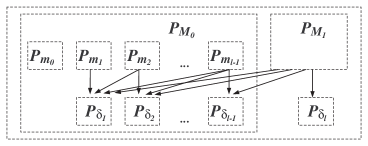
Figure 5. Scheme for a circuit representing $M_{0}+2^{-\sigma_{1}}M_{1}$.

∎

Proposition 5.4 (Complexity of processing in $B_{(1,2)}$).

It takes

$$O{\left(k{\left(\sum_{j=0}^{k}(|V({\mathcal{P}}_{m_{j}})|+|M({\mathcal{P}}_{m_{j}})|)+\sum_{j=1}^{k}|V({\mathcal{P}}_{\delta_{j}})|\right)}^{3}\right)}$$

operations to determine if (7) is equivalent to a sequence $(a,{\mathcal{P}})$ or a sequence $(t,{\mathcal{P}})$. If (7) is equivalent to a sequence $(a,{\mathcal{P}})$ then ${\mathcal{P}}$ satisfies:

$$|V({\mathcal{P}})|\leq\sum_{j=0}^{k}(|V({\mathcal{P}}_{m_{j}})|+|M({\mathcal{P}}_{m_{j}})|)+\sum_{j=1}^{k}|V({\mathcal{P}}_{\delta_{j}})|\mbox{ and }|M({\mathcal{P}})|=\sum_{j=0}^{k}|M({\mathcal{P}}_{m_{j}})|.$$

If (7) is equivalent to a sequence $(t,{\mathcal{P}})$ then ${\mathcal{P}}$ satisfies:

$$|V({\mathcal{P}})|=\sum_{j=1}^{k}|V({\mathcal{P}}_{\delta_{j}})|\mbox{ and }|M({\mathcal{P}})|=\sum_{j=1}^{k}|M({\mathcal{P}}_{\delta_{j}})|.$$

Proof.

The bounds on $|V({\mathcal{P}})|$ and $|M({\mathcal{P}})|$ for both cases follow from Propositions 5.1 and 5.3. Furthermore, at every step in the process all power circuits in the sequence (7) have the number of vertices bounded by $\sum_{j=0}^{k}(|V({\mathcal{P}}_{m_{j}})|+|M({\mathcal{P}}_{m_{j}})|)+\sum_{j=1}^{k}|V({\mathcal{P}}_{\delta_{j}})|$. Hence, it takes up to

$$O{\left({\left(\sum_{j=0}^{k}(|V({\mathcal{P}}_{m_{j}})|+|M({\mathcal{P}}_{m_{j}})|)+\sum_{j=1}^{k}|V({\mathcal{P}}_{\delta_{j}})|\right)}^{3}\right)}$$

operations to check if conditions of Propositions 5.1 and 5.3 hold at every step. The algorithm performs $O(k)$ transformations and hence the claimed bound on complexity. ∎

5.2. Complexity estimate for Algorithm 5

Theorem 5.5.

Algorithm 5 solves the Word problem for $G_{(1,2)}$ in time $O(|w|^{7})$.

Proof.

Let $w=w(a,b,t)$ be a reduced word over the alphabet $\{a,b,t\}$. First, Algorithm 5 constructs a power sequence ${\mathcal{S}}$ for $w$. As described in [23] it is straightforward to construct circuits for numbers $m_{i},\varepsilon_{i},\delta_{i}$. Clearly, the total number of vertices for circuits $m_{i},\varepsilon_{i},\delta_{i}$ is not greater than $2|w|$. This can be done in $O(|w|)$ steps.

In the loop 3–10 Algorithm 5 determines what subsequences ${\mathcal{S}}_{g_{i}}$ can be shortened into $(a,{\mathcal{P}})$ or $(t,{\mathcal{P}})$. By Proposition 5.4 this can be done in time

$$O{\left(|g_{i}|\cdot{\left(|V({\mathcal{P}}_{g_{i}})|+|M({\mathcal{P}}_{g_{i}})|\right)}^{3}\right)}$$

and the obtained circuit ${\mathcal{P}}$ satisfies

$$|V({\mathcal{P}})|\leq V({\mathcal{S}}_{g_{i}})+M({\mathcal{S}}_{g_{i}})\mbox{ and }|M({\mathcal{P}})|\leq M({\mathcal{S}}_{g_{i}}).$$

Hence, a single transformation on a step 5 or 8

• does not increase the total number of marked vertices in ${\mathcal{S}}$;

• can increase the total number of vertices by the number of marked vertices.

Therefore, in the worst case steps 5 and 8 are performed on a sequence $S_{g_{i}}$ of size $|V(S_{g_{i}})|=O(|w|^{2})$. Algorithm 5 performs up to $|w|$ steps 5 and 8. Hence the result. ∎

References

- [1] G. Baumslag, On generalized free products, Math. Z. 78 (1962), pp. 423–438.
- [2] by same author, A non-cyclic one-relator group all of whose finite factor groups are cyclic, J. Australian Math. Soc. 10 (1969), pp. 497–498.
- [3] by same author, Some problems on one-relator groups. Proceedings of the Second International Conference on the Theory of Groups, Lecture Notes in Computer Science 372. Springer, Berlin, 1974.
- [4] G. Baumslag, C. Miller, and D. Troeger, Reflections on the residual finiteness of one-relator groups, Groups Geom. Dyn. 1 (2007), pp. 209–219.
- [5] G. Baumslag, A. G. Myasnikov, and V. Shpilrain, Open problems in combinatorial group theory. Second Edition. Combinatorial and geometric group theory, Contemporary Mathematics 296, pp. 1–38. American Mathematical Society, 2002.
- [6] G. Baumslag and D. Solitar, Some two-generator one-relator non-Hopfian groups, Bull. Amer. Math. Soc. 68 (1962), pp. 199–201.
- [7] M. Bestvina and M. Feighn, A combination theorem for negatively curved groups, J. Differential Geom. 35 (1992), pp. 85–101.
- [8] J. L. Britton, The word problem, Ann. of Math. 77 (1963), pp. 16–32.
- [9] Groves D. and S. Hermiller, Isoperimetric Inequalities for Soluble Groups , Geometriae Dedicata 88 (2001), pp. 239–254.
- [10] C. Drutu and M. Sapir, Non-linear residually finite groups, J. Algebra 284 (2005), pp. 174–178.
- [11] D. B. A. Epstein, J. W. Cannon, D. F. Holt, S. V. F. Levy, M. S. Paterson, and W. P. Thurston, Word processing in groups. Jones and Bartlett Publishers, 1992.
- [12] S. Gersten, The double exponential theorem for isodiametric and isoperimetric functions, Int. J. Algebr. Comput. 1 (1991), pp. 321–327.
- [13] S. M. Gersten, Dehn functions and l1-norms of finite presentations. Algorithms and Classification in Combinatorial Group Theory, pp. 195–225. Springer, Berlin, 1992.
- [14] M. Greendlinger, Dehn’s algorithm for the word problem, Comm. Pure and Appl. Math. 13 (1960), pp. 67–83.
- [15] S. Ivanov and P. Schupp, On the hyperbolicity of small cancelation groups and one-relator groups, Trans. Amer. Math. Soc. 350 (1998), pp. 1851–1894.
- [16] O. Kharlampovich and A. Myasnikov, Hyperbolic groups and free constructions, Trans. Amer. Math. Soc. 350 (1998), pp. 571–613.
- [17] R. Lipton and Y. Zalstein, Word Problems Solvable in Logspace, JACM 24 (1977), pp. 522–526.
- [18] R. Lyndon and P. Schupp, Combinatorial Group Theory, Classics in Mathematics. Springer, 2001.
- [19] W. Magnus, Das Identitätsproblem für Gruppen mit einer definierenden Relation, Math. Ann. 106 (1932), pp. 295–307.
- [20] W. Magnus, A. Karrass, and D. Solitar, Combinatorial Group Theory. Springer-Verlag, 1977.
- [21] J. McCool, On a question of Remeslennikov, Glasgow Math. J. 43 (2001), pp. 123–124.
- [22] S. Meskin, Nonresidually finite one-relator groups, Trans. Amer. Math. Soc. 164 (1972), pp. 105–114.
- [23] A. G. Miasnikov, A. Ushakov, and Don-Wook Won, Power Circuits, Exponential Algebra, and Time Complexity, preprint. Available at http://arxiv.org/abs/1006.2570, 2010.
- [24] B. B. Newman, Some results on one-relator groups, Bull. Amer. Math. Soc. 74 (1968), pp. 568–571.
- [25] A. N. Platonov, Isoparametric function of the Baumslag-Gersten group, (Russian) Vestnik Moskov. Univ. Ser. I Mat. Mekh. (2004), pp. 12–17.
- [26] R. Vol’vachev, Linear representation of certain groups with one relation, Vestsi Akad. Navuk BSSR Ser. Fiz.-Mat. Navuk 124 (1985), pp. 3–11.
- [27] B. A. F. Wehrfritz, Generalized free products of linear groups, Proc. London Math. Soc. 27 (1973), pp. 402–424.
- [28] D. Wise, Research announcement: The structure of groups with a quasiconvex hierarchy, Electronic Research Announcements in Mathematical Sciences 16 (2009), pp. 44–55.