Abstract

We analyse a $p+ip$-wave pairing BCS Hamiltonian, coupled to a single bosonic degree of freedom representing a molecular condensate, and investigate the nature of the BEC-BCS crossover for this system. For a suitable restriction on the coupling parameters, we show that the model is integrable and we derive the exact solution by the algebraic Bethe ansatz. In this manner we also obtain explicit formulae for correlation functions and compute these for several cases. We find that the crossover between the BEC state and the strong pairing $p+ip$ phase is smooth for this model, with no intermediate quantum phase transition.

Keywords: BCS model; integrable systems; Bethe ansatz; correlation functions.

1 Introduction

Progress in cold atom physics has yielded many studies into the nature of the BEC-BCS crossover [1]. Early theoretical accounts emphasized the need to study Hamiltonians which explicitly incorporate coupling between Cooper pairs of atoms and bosonic molecular modes [2]. Several works extended this approach to the case of $p$-wave paired systems [3], a scenario that is experimentally accessible [4]. Currently there is substantial interest in $p+ip$-wave paired systems [5], which has been primarily motivated by the seminal work of Read and Green [6] who illustrated the topological distinctions of the quantum phases occuring in this setting. Our objective here is to study a $p+ip$-wave pairing Hamitonian which is coupled to a bosonic molecular degree of freedom to investigate the BEC-BCS crossover in this context. Our approach is to employ exact Bethe ansatz methods for the analysis.

There have been many exact analyses of the $s$-wave pairing reduced BCS Hamiltonian using the solution provided by Richardson [7]. These works were particularly prevalent in the wake of experiments conducted on metallic nanograins [8]. A comprehensive understanding of the model’s mathematical property of integrability has been developed [9] which has lead in particular to some in-depth investigations through the use of exact computation of correlation functions [10]. There have been efforts to extend these integrable methods to investigate models where there is coupling between Cooper pairs and bosonic molecular modes [11]. Generally, these examples fall into a class of generalised Dicke/Tavis-Cummings type integrable models [12]. They have the shortcoming that the pair-pair scattering terms found in the Hamiltonians of [2] are not present, with only pair-molecule scattering terms appearing.

More recently it has been established that an integrable model also exists for $p+ip$-wave pairing [13, 14, 15, 16]. Integrability in this instance stems from a trigonometric solution of the classical Yang–Baxter equation, in contrast to the rational solution associated with the integrable $s$-wave case. We will show below that an extension of this model through coupling to a bosonic degree of freedom, whilst maintaining pair-pair scattering interactions, is integrable for some restriction of the coupling parameter space. We will derive the exact solution of the Hamiltonian’s energy spectrum and certain correlation functions and use these results to study the BEC-BCS crossover.

This paper is organized as follows. We begin Section 2 by introducing a general Hamiltonian describing a $p+ip$-wave pairing BCS model coupled to a bosonic molecular degree of freedom. Subsection 2.1 discusses the limiting case of the uncoupled system, in which the extreme limits of BEC and strong pairing BCS ground states are found. Subsection 2.2 establishes suitable constraints on the Hamiltonian’s coupling parameters for which the system is integrable, while subsection 2.3 develops the exact solution via algebraic Bethe ansatz methods. The ground-state root structure of the Bethe ansatz equations is determined in subsection 2.4, and based on these results it is shown in 2.5 that the ground-state wavefunction topology is trivial so no topological phase transition exists in the integrable case. Since the integrable case connects the extreme BEC and strong pairing BCS ground states, these belong to the same quantum phase. Section 3 is devoted to the study of correlation function. Subsection 3.1 deals with one-point correlation functions and particular attention is given to the boson fraction expectation value. Subsection 3.2 deals with two-point functions and the boson-Cooper pair fluctuations are studied in some depth. Conclusions are summarised in Section 4. An Appendix on a mean-field treatment of the model is also included.

2 Model Hamiltonian

We consider a 2-dimensional $p+ip$-wave pairing BCS model coupled to a single bosonic degree of freedom where the Hamiltonian of the model is

$$H = \delta b^{\dagger}b+\sum_{\bf k}{{\bf k}^{2}\over 2m}c^{\dagger}_{\bf k}c_{\bf k}-{G\over 4}\sum_{{\bf k}\neq\pm{\bf k}^{\prime}}(k_{x}-ik_{y})(k^{\prime}_{x}+ik^{\prime}_{y})c^{\dagger}_{\bf k}c^{\dagger}_{-{\bf k}}c_{\bf k^{\prime}}c_{-{\bf k}^{\prime}}$$ (1)

$$\mbox{}-{K\over 2}\sum_{\bf k}\left((k_{x}-ik_{y})c^{\dagger}_{\bf k}c^{\dagger}_{-{\bf k}}b+{\rm h.c.}\right).$$

One sees that when $\delta=K=0$, the Hamiltonian becomes the integrable $p+ip$ pairing BCS model [13] with $c_{\bf k}$ and $c^{\dagger}_{\bf k}$ being destruction and creation operators of 2-dimensional polarised fermions, ${\bf k}$ and $m$ the momentum and mass of the fermions and $G$ a coupling constant which is positive for an attractive $p+ip$ interaction. In the above Hamiltonian, the bosonic mode with destruction and creation operators $b$, $b^{\dagger}$ is associated to a zero-momentum molecular condensate. The interconversion between Cooper pairs and molecules is controlled by the coupling $K$. The sign of $K$ is not important since it can be changed by the unitary transformation $b\rightarrow-b$. Included in the Hamiltonian is the detuning $\delta$ which accounts for the energy splitting by a magnetic field due to the difference between the magnetic moment of the molecules and that of the Cooper pairs. Hereafter we set $m=1$. This model is integrable if we set $\delta=-F^{2}G,K=FG$ with $F$ being a free variable, which will be proved below. Before considering that, it is useful to first examine the ground-state phases of the uncoupled system.

2.1 Limiting case of the uncoupled system

Setting $\delta=K=0$ the Hamiltonian (1), restricted to the Hilbert subspace where the bosonic degree of freedom is in the vacuum state, is the $p+ip$ model. For the extended model (1), with $\delta=K=0$ on the full Hilbert space, the ground state of the system is of the form

$$|\phi\rangle=|\psi_{BCS}\rangle\otimes|N_{b}\rangle$$ (2)

where $|\psi_{BCS}\rangle$ is a ground state associated with the $p+ip$ Hamiltonian and $|N_{b}\rangle$ is a bosonic number state. For the ground state we need to consider the optimal choice of the boson number $N_{b}$ which yields the lowest energy. Since the detuning is zero in this limit, the ground state will be one which provides the mimimum energy of $|\psi_{BCS}\rangle$ with respect to variations of the Cooper pair number.

To elucidate the ground state structure in this limit we recall results from [15] for the $p+ip$ model, which has three ground-state phases called weak coupling, weak pairing, and strong pairing. Letting $N_{C}$ denote the number of Cooper pairs, we set $x_{C}=N_{C}/{\cal L}$ as the filling fraction, and $g=G{\cal L}$. Throughout, $2{\cal L}$ denotes the total number of momentum levels such that ${\cal L}$ is the number of momentum pairs. The three phases are characterized by the constraints shown in Table 1. In the weak coupling phase the ground-state energy is positive, on the Moore-Read line it is zero, and in all other cases it is negative. Ground states in the weak pairing and strong pairing phases, with filling fractions $x_{C}^{W}$, $x_{C}^{S}$, are dual whenever $x_{C}^{W}+x_{C}^{S}=1-g^{-1},$ with the two ground states having the same energy. The Read-Green state is self-dual. The Read-Green condition $x_{C}=(1-{g^{-1}})/2$ gives the state with the lowest possible energy, for all $g>1$, with respect to variations in $x_{C}$. For $g<1$, corresponding to the weak coupling phase, the lowest possible energy is given by the vacuum since all ground states with $x_{C}>0$ have positive energy in this phase. The only phase for which the ground-state wavefunction is topologically non-trivial is the weak pairing phase [15].

Phase	Filling fraction $x_{C}$
weak coupling	$x_{C}>1-{g^{-1}}$
Moore-Read line	$x_{C}=1-{g^{-1}}$
weak pairing	$(1-{g^{-1}})/2<x_{C}<1-{g^{-1}}$
Read-Green line	$x_{C}=(1-{g^{-1}})/2$
strong pairing	$x_{C}<(1-{g^{-1}})/2$

Table 1.- Ground-state phases of the $p+ip$ model.

In view of the above we can determine the ground-state structure of (1) when $\delta=K=0$. We let $x=x_{b}+x_{C}$ denote the filling fraction of the system, where $x_{b}=N_{b}/{\cal L}$. If $g<1$ all $p+ip$ states with $x_{C}>0$ have positive energy, so the ground state is obtained by choosing $x_{b}=x$ and $x_{C}=0$, giving a pure BEC state for (2) with zero energy. For $g>1$ the $p+ip$ ground states have negative energy. If $x>(1-g^{-1})/2$ we choose $x_{C}=(1-g^{-1})/2$ so the $p+ip$ state is the Read-Green state, which has the minimum energy with respect to variations of $x_{C}$. This then leaves $x_{b}=x-(1-g^{-1})/2$ so (2) is mixed. Finally if $x<(1-g^{-1})/2$ the $p+ip$ state is in the strong pairing phase. The energy is miminised by choosing $x_{b}=0$. This leads to the classification shown in Table 2.

Phase	$g$	Filling fraction $x$	$|\psi_{BCS}\rangle$	$N_{b}$
BEC	$g<1$	all	vacuum	$N$
Mixed	$g>1$	$x>(1-g^{-1})/2$	Read-Green	$0<N_{b}<N$
BCS	$g>1$	$x<(1-g^{-1})/2$	strong pairing	$0$

Table 2.- Ground-state phases of the Hamiltonian (1) for $\delta=K=0$.

To investigate the crossover between the BEC state and the BCS state we may start with $g>1$ and $K=\delta=0$ in the Hamiltonian (1) so the ground state consists of the strong pairing $p+ip$ state and the bosonic vacuum provided $x<(1-g^{-1})/2$. By turning on $K$ and $\delta$ we obtain an interacting system of Cooper pairs and bosons. Next we vary $g$ such that $g<1$, and then turn off $K$ and $\delta$. The ground state will now consist of the $p+ip$ vacuum and a bosonic number state. The question we ask is whether the system experiences a phase transition as we pass from the strong pairing BCS state to the BEC state in this manner. Importantly, the coupling parameters can be varied such that the Hamiltonian remains integrable as we move between the BEC state and the strong pairing BCS state.

2.2 Integrability conditions for the coupled system

It is convenient to first perform a transformation on the Hamiltonian (1). We enumerate the complex momenta ${\bf k}=k_{x}+ik_{y}$, with $k_{y}$ in the upper half-plane, by integers $j=1,...,{\cal L}$. Implementing the canonical transformation

$$s_{j}={k_{x}-ik_{y}\over|{\bf k}|}c_{\bf k}c_{-{\bf k}},\quad\quad z_{j}=|{\bf k}|,$$

we may rewrite the Hamiltonian (1) as

$$H=\delta N_{b}+(1+G)H_{0}-GQ^{\dagger}Q-KQ^{\dagger}b-Kb^{\dagger}Q,$$ (3)

where we have defined

$$N_{b}=b^{\dagger}b,\qquad\qquad\,{N}_{j}=s_{j}^{\dagger}s_{j},\,\,\qquad j=1,\ldots,{\cal L},$$

$$H_{0}=\sum_{j=1}^{\cal L}z_{j}^{2}N_{j},\quad\,\,\,\,Q^{\dagger}=\sum_{j=1}^{\cal L}z_{j}s_{j}^{\dagger}.$$ (4)

provided we restrict to the subspace of the Hilbert space which excludes blocked states (see [8] for a discussion of the blocking effect). This restriction is sufficient to study the ground-state properties when the total fermion number is even. We use ${N}$ to stand for the pair number operator which is the sum of the boson and pairing number operators; namely, ${N}={N}_{b}+{N}_{c}$ with ${N}_{c}=\sum_{j=1}^{\cal L}{N}_{j}$. We note that ${N}$ commutes with the Hamiltonian (1). This allows us to block diagonalise the Hamiltonian into sectors labelled by the eigenvalues of $N$, which are non-negative integers. Hereafter we will adopt the practice to interchangably use the symbol $N$ to denote the pair number operator and its eigenvalues.

Now we show that for a suitable restriction on the coupling parameters of (1) the model is integrable. The integrable manifold is defined by the relations

$$\delta=-F^{2}G,\,\qquad K=FG$$ (5)

with $F$ being a free variable. Under this constraint, the Hamiltonian (1) becomes

$$H = -F^{2}GN_{b}+(1+G)H_{0}-GQ^{\dagger}Q-FGQ^{\dagger}b-FGb^{\dagger}Q.$$ (6)

We will prove the integrability of the above Hamiltonian by using the Quantum Inverse Scattering Method [17]. Our approach is a generalisation of the method detailed in [15].

Let $V$ be the 2-dimensional $U_{q}(sl(2))$-module and $R(\lambda)\in\mbox{End}(V\otimes V)$ the six-vertex solution of the Yang-Baxter equation

$$R_{12}(\lambda/\mu)R_{13}(\lambda)R_{23}(\mu)=R_{23}(\mu)R_{13}(\lambda)R_{12}(\lambda/\mu)$$

acting on the three-fold space $V\otimes V\otimes V$. The $R$-matrix, which depends on the spectral parameter $\lambda$ and the crossing parameter $q$, explicitly reads

$$R(\lambda)=\left(\begin{array}[]{ccccc}\lambda q^{2}-\lambda^{-1}q^{-2}&0&|&0&0\\ 0&\lambda-\lambda^{-1}&|&q^{2}-q^{-2}&0\\ -&-&\mbox{}&-&-\\ 0&q^{2}-q^{-2}&|&\lambda-\lambda^{-1}&0\\ 0&0&|&0&\lambda q^{2}-\lambda^{-1}q^{-2}\end{array}\right).$$

We construct the Yang-Baxter algebra by using the $R$-matrix and the $L$-operator $L(\lambda)$ through the Yang-Baxter relation (YBR)

$$R_{12}(\lambda/\mu)L_{1j}(\lambda)L_{2j}(\mu)=L_{2j}(\mu)L_{1j}(\lambda)R_{12}(\lambda/\mu).$$ (8)

Here $L_{\alpha j}(\lambda)\in\mbox{End}(V\otimes V)$ is a $2\times 2$ matrix of operators. In the framework of quantum integrable systems, the subscript $\alpha$ labels the auxiliary space, while entries of the matrix are operators acting on the $j$th quantum space.

A well-known $L$-operator is realised by the $R$-matrix itself which, using local creation $s^{\dagger}$ and destruction operators $s$, is expressed as

$$L_{\sigma i}(\lambda) = \left(\begin{array}[]{cc}\lambda q^{(2{N}_{i}-1)}-\lambda^{-1}q^{-(2{N}_{i}-1)}&(q^{2}-q^{-2})s_{i}\\ (q^{2}-q^{-2})s_{i}^{\dagger}&\lambda q^{-(2{N}_{i}-1)}-\lambda^{-1}q^{(2{N}_{i}-1)}\end{array}\right)_{(\sigma)}$$

where ${N}_{i}$ is the local number operator with the definition ${N}_{i}=s_{i}^{\dagger}s_{i}$. The operators $s_{i}^{\dagger}$, $s_{i}$ and ${N}_{i}$ are generators of the quantum algebra $U_{q}(sl(2))$. In the 2-dimensional representation they satisfy the relation

$$[s_{i},s_{j}^{\dagger}]=\delta_{ij}(I-2{N}_{i}).$$

A realisation of the $L$-operator using the $q$-boson algebra was given by Kundu [18]:

$$\widetilde{L}_{\sigma b}(\lambda)=\left(\begin{array}[]{cc}\lambda q^{2N_{b}}-i\lambda^{-1}q^{-2(N_{b}+1)}&-e^{i\pi/4}(q^{4}-q^{-4})^{1/2}b\\ -e^{i\pi/4}(q^{4}-q^{-4})^{1/2}b^{\dagger}&\lambda q^{-2N_{b}}+i\lambda^{-1}q^{2(N_{b}+1)}\end{array}\right)_{(\sigma)}.$$

The subscript $b$ in the $L$-operator $\widetilde{L}_{\sigma b}(\lambda)$ stands for the bosonic quantum space. The local $q$-boson operators $b_{q}$, $b_{q}^{\dagger}$ and $N_{b}=b_{q}^{\dagger}b_{q}$ have the following commutation relation

$$[b_{q},b_{q}^{\dagger}]={q^{2(2N_{b}+1)}+q^{-2(2N_{b}+1)}\over q^{2}+q^{-2}}.$$

It can be seen that when $q\rightarrow 1$, $b_{q}$ and $b_{q}^{\dagger}$ become the usual bosonic destruction and creation operators $b$ and $b^{\dagger}$. With the help of the mapping

$$\widetilde{L}_{\sigma b}(\lambda)\rightarrow-e^{-i\pi/4}(q^{4}-q^{-4})^{1/2}\mbox{diag}\left(q^{1/2},q^{-1/2}\right)\cdot\widetilde{L}_{\sigma b}(\lambda)\cdot\mbox{diag}\left(q^{1/2},q^{-1/2}\right)$$

and the variable shift $\lambda\rightarrow-e^{-i\pi/4}(q^{4}-q^{-4})^{1/2}\lambda$ the $L$-operator, which still satisfies (8), becomes

$$\widetilde{L}_{\sigma b}(\lambda)=\left(\begin{array}[]{cc}(\widetilde{L}_{\sigma b})_{11}&(\widetilde{L}_{\sigma b})_{12}\\ (\widetilde{L}_{\sigma b})_{21}&(\widetilde{L}_{\sigma b})_{22}\end{array}\right)_{(\sigma)},$$

where the elements are

$$(\widetilde{L}_{\sigma b})_{11}=\lambda q^{(2N_{b}+1)}-(q^{4}-q^{-4})\lambda^{-1}q^{-(2N_{b}+1)},$$

$$(\widetilde{L}_{\sigma b})_{12}=(q^{4}-q^{-4})b_{q},$$

$$(\widetilde{L}_{\sigma b})_{21}=(q^{4}-q^{-4})b^{\dagger}_{q},$$

$$(\widetilde{L}_{\sigma b})_{22}=\lambda q^{-(2N_{b}+1)}+(q^{4}-q^{-4})\lambda^{-1}q^{(2N_{b}+1)}.$$

Now we define the monodromy matrix

$$T_{\sigma}(\lambda) = g_{\sigma}\widetilde{L}_{\sigma b}(\lambda z_{b}^{-1})L_{\sigma{\cal L}}(\lambda z_{\cal L}^{-1})\cdots L_{\sigma 2}(\lambda z_{2}^{-1})L_{\sigma 1}(\lambda z_{1}^{-1}))$$ (12)

with the diagonal matrix $g_{\sigma}=\mbox{diag}(e^{-i\alpha},e^{i\alpha})_{(\sigma)}$. Using the YBR (8), the following equation holds for the monodromy matrix

$$R_{\sigma\rho}(\lambda/\mu)T_{\sigma}(\lambda)T_{\rho}(\mu)=T_{\rho}(\mu)T_{\sigma}(\lambda)R_{\sigma\rho}(\lambda/\mu).$$

This relation ensures the commutation relation

$$[t(\lambda),t(\mu)]=0,\quad\forall\,\,\lambda,\mu$$

where $t(\lambda)$ is the transfer matrix defined by $t(\lambda)={\rm tr}_{\sigma}\left[T_{\sigma}(\lambda)\right]$.

Expanding the transfer matrix $t(\lambda)$ in orders of the spectral parameter $\lambda$

$$t(\lambda)=\sum_{i=-{\cal L}-1}^{{\cal L}+1}t^{(i)}\lambda^{i},$$

we find that the coefficients commute with each other

$$[t^{(i)},t^{(j)}]=0$$

for all $i,j$. In this manner we may construct an integrable system by using the coefficients $t^{(i)}$. The leading terms of the expansion are

$$t^{({\cal L}+1)} = \left(z_{b}^{-1}\prod_{i=1}^{\cal L}z_{i}^{-1}\right)\left(e^{-i\alpha}q^{2{N}-{\cal L}+1}+h.c.\right),$$

$$t^{({\cal L})} = 0,$$

$$t^{({\cal L}-1)} = -\left(z_{b}^{-1}\prod_{i=1}^{\cal L}z_{i}^{-1}\right)\sum_{j=1}^{\cal L}z_{j}^{2}\left(e^{-i\alpha}q^{2{N}-{\cal L}+1}q^{-(4{N}_{j}-2)}+h.c.\right)$$

$$\mbox{}-z_{b}^{2}(q^{4}-q^{-4})\left(z_{b}^{-1}\prod_{i=1}^{\cal L}z_{i}^{-1}\right)\left(e^{-i\alpha}q^{2{N}-{\cal L}+1}q^{-(4N_{b}+2)}-h.c\right)$$

$$\mbox{}+(q^{2}-q^{-2})^{2}\left(z_{b}^{-1}\prod_{i=1}^{\cal L}z_{i}^{-1}\right)$$

$$\quad\quad\times\sum_{j<k}^{\cal L}z_{j}z_{k}\left(e^{-i\alpha}q^{2{N}-{\cal L}+1}\prod_{l=j+1}^{k-1}q^{-(4{N}_{l}-2)}s_{k}s_{j}^{\dagger}+h.c.\right)$$

$$\mbox{}+(q^{2}-q^{-2})^{2}(q^{2}+q^{-2})\left(z_{b}^{-1}\prod_{i=1}^{\cal L}z_{i}^{-1}\right)$$

$$\quad\quad\times\sum_{j=1}^{\cal L}z_{b}z_{j}\left(e^{-i\alpha}q^{2{N}-{\cal L}+1}q^{-2N_{b}-1}\prod_{l=j+1}^{\cal L}q^{-(4{N}_{l}-2)}b_{q}s_{j}^{\dagger}+h.c.\right).$$

Introducing the notation

$$q=e^{i\beta},\quad\beta=\eta p,\quad\alpha-\beta(2{N}-{\cal L}+1)={\eta t},$$

we define a Hamiltonian $\widetilde{H}$ by using the coefficient $t^{({\cal L}-1)}$:

$$\widetilde{H} = (q^{2}-q^{-2})^{-2}z_{b}\prod_{i=1}^{\cal L}z_{i}\,\,t^{({\cal L}-1)}$$ (13)

$$= -{1\over\sin^{2}(2\eta p)}\sum_{j=1}^{\cal L}z_{j}^{2}\sin^{2}\left(\eta{t+4p{N}_{j}-2p\over 2}\right)+{1\over 2\sin^{2}(2\eta p)}\sum_{j=1}^{\cal L}z_{j}^{2}$$

$$\mbox{}+2z_{b}^{2}\cot(2\eta p)\sin(\eta(t+4pN_{b}+2p))$$

$$\mbox{}+\sum_{j<k}^{\cal L}z_{j}z_{k}\left(e^{-i\eta t}\prod_{l=j+1}^{k-1}e^{-i\eta p(4{N}_{l}-2)}s_{k}s_{j}^{\dagger}+e^{i\eta t}\prod_{l=j+1}^{k-1}e^{i\eta p(4{N}_{l}-2)}s_{k}^{\dagger}s_{j}\right)$$

$$\mbox{}+2\cos(2\eta p)\sum_{j=1}^{\cal L}z_{b}z_{j}\left(e^{-i\eta(t+2pN_{b}+p)}\prod_{l=j+1}^{\cal L}e^{-i\eta(4{N}_{l}-2)}b_{q}s_{j}^{\dagger}\right.$$

$$\mbox{}\quad\quad+\left.e^{i\eta(t+2pN_{b}+p)}\prod_{l=j+1}^{\cal L}e^{i\eta(4{N}_{l}-2)}b^{\dagger}_{q}s_{j}\right).$$

Let $G=2p/t$ and $F=2z_{b}$. Taking the limit $\eta\rightarrow 0$, we obtain the following Hamiltonian

$$H = -G\lim_{\eta\rightarrow 0}\left(\widetilde{H}-{1\over 2\sin^{2}(2\eta p)}\sum_{j=1}^{\cal L}z_{j}^{2}+\sum_{j=1}^{\cal L}z_{j}^{2}{(t-2p)^{2}\over 16p^{2}}-{z_{b}^{2}(t+2p)\over p}\right)$$

$$= \sum_{j=1}^{\cal L}z_{j}^{2}{N}_{j}-{F^{2}G}N_{b}-G\sum_{j<k}^{\cal L}z_{j}z_{k}\left(s_{k}s_{j}^{\dagger}+h.c\right)-{FG}\sum_{j=1}^{\cal L}z_{j}\left(bs_{j}^{\dagger}+h.c\right).$$

Utilizing (4) we find that (LABEL:de:Hamiltonian-p) is equivalent to (6). Therefore we have established that the constraint (5) defines an integrable manifold in the coupling parameter space of (1).

2.3 Algebraic Bethe ansatz solution

The eigenvalues of the Hamiltonian (LABEL:de:Hamiltonian-p) can be obtained by using the algebraic Bethe ansatz. Again, we follow the procedure of [15] and only present the main results. Rewriting the monodromy matrix $T_{\sigma}(\lambda)$ (12) by using global quantum operators $A(\lambda),B(\lambda),C(\lambda)$ and $D(\lambda)$ defined by

$$T(\lambda)=\left(\begin{array}[]{cc}A(\lambda)&B(\lambda)\\ C(\lambda)&D(\lambda)\end{array}\right)_{(\sigma)},$$

the transfer matrix $t(\lambda)$ becomes

$$t(\lambda)={\rm tr}_{\sigma}\left[T_{\sigma}(\lambda)\right]=A(\lambda)+D(\lambda).$$

The Bethe states of the system are defined by

$$|\Phi(\{\mu\})\rangle=\prod_{i=1}^{N}C(\mu_{i})|0\rangle,$$

where $|0\rangle$ is the vacuum state with the definition

$$b|0\rangle=s_{i}|0\rangle=0$$

for all $i=1,\ldots,{\cal L}.$

By using the standard algebraic Bethe ansatz method [17], the eigenvalues of the Hamiltonian (13) are given by

$$\widetilde{E} = 2z_{b}^{2}\cot(2\eta p)\sin(\eta(t+2p))-\left({\sin^{2}(\eta(-t+2p)/2)\over\sin^{2}(2\eta p)}\right)\sum_{i=1}^{\cal L}z_{i}^{2}$$

$$\mbox{}+{1\over 2\sin^{2}(2\eta p)}\sum_{i=1}^{\cal L}z_{i}^{2}-{\sin(\eta(t+2p))\over\sin(2\eta p)}\sum_{j=1}^{N}\mu_{j}^{2}.$$

Here, the parameters $\mu_{j}$ $(j=1,2,\ldots,{N})$ satisfy the following Bethe ansatz equations

$$e^{-2i\alpha}{\mu_{j}z_{b}^{-1}q-(q^{4}-q^{-4})\mu_{j}^{-1}z_{b}q^{-1}\over\mu_{j}z_{b}^{-1}q^{-1}+(q^{4}-q^{-4})\mu_{j}^{-1}z_{b}q}\prod_{i=1}^{\cal L}{\mu_{j}z_{i}^{-1}q^{-1}-\mu_{j}^{-1}z_{i}q\over\mu_{j}z_{i}^{-1}q-\mu_{j}^{-1}z_{i}q^{-1}}$$

$$=\prod_{k\neq j}^{N}{\mu_{j}\mu_{k}^{-1}q^{-2}-\mu_{j}^{-1}\mu_{k}q^{2}\over\mu_{j}\mu_{k}^{-1}q^{2}-\mu_{j}^{-1}\mu_{k}q^{-2}}\quad.$$

Taking the limit $\eta\rightarrow 0$, we obtain the eigenvalues of (LABEL:de:Hamiltonian-p):

$$E=(1+G)\sum_{j=1}^{N}\mu_{j}^{2}$$

subject to the Bethe ansatz equations

$${G^{-1}+2{N}-{\cal L}-1\over\mu_{j}^{2}}+{4z_{b}^{2}\over\mu_{j}^{4}}+\sum_{i=1}^{\cal L}{1\over\mu_{j}^{2}-z_{i}^{2}}=\sum_{k\neq j}^{N}{2\over\mu_{j}^{2}-\mu_{k}^{2}}$$

for $j=1,\ldots,{N}$. For convenience, throughout the remainder of the paper we will simplify notation by making the substitutions

$$\lambda_{j}^{2}\mapsto\lambda_{j},\quad\quad\mu_{j}^{2}\mapsto\mu_{j},$$

such that the Bethe ansatz equations take the form

$${G^{-1}+2{N}-{\cal L}-1\over\mu_{j}}+{4z_{b}^{2}\over\mu_{j}^{2}}+\sum_{i=1}^{\cal L}{1\over\mu_{j}-z_{i}^{2}}=\sum_{k\neq j}^{N}{2\over\mu_{j}-\mu_{k}}.\quad\quad$$ (16)

In the $\eta\rightarrow 0$ limit the Bethe states and their dual states are defined by

$$|\phi(\{\lambda\})\rangle=\prod_{j=1}^{N}{\cal C}(\lambda_{j})|0\rangle,$$ (17)

$$\langle\phi(\{\mu\})|=\langle 0|\prod_{j=1}^{N}{\cal B}(\mu_{j}),$$

where ${\cal C}$ and ${\cal B}$ are the global creation and destruction operators given by

$${\cal C}(\lambda) = {2z_{b}b^{\dagger}\over\lambda}+\sum_{j=1}^{\cal L}{z_{j}s_{j}^{\dagger}\over\lambda-z_{j}^{2}},$$ (18)

$${\cal B}(\mu) = {2z_{b}b\over\mu}+\sum_{j=1}^{\cal L}{z_{j}s_{j}\over\mu-z_{j}^{2}}$$ (19)

2.4 Ground-state root structure

It is necessary to understand the character of the roots of (16) which correspond to the ground state of the model. By adding an appropriate constant term to (6), all matrix elements are real and negative on each sector with fixed ${N}$. From numerical studies of (16) we find solutions for which all the roots $\lambda_{j}$ are real and negative. From (18), and an appropriate rescaling ${\cal C}(\lambda)\rightarrow-{\cal C}(\lambda)$, we see that these roots give rise to an eigenvector with positive components. This eigenvector necessarily corresponds to the ground state as a result of the Perron-Frobenius theorem. This theorem also tells us that there is a unique solution set with the property that all $\lambda_{j}$ are real and negative.

While we are unable to prove existence of a solution set with the property of all roots being real and negative in a general finite system, we can establish existence of such a set in the thermodyanamic limit. To analyze the thermodynamic limit of the model, ${\cal L}\rightarrow\infty$, $N\rightarrow\infty$ such that the filling fraction $x=N/{\cal L}$ remains finite, we follow the approach of [15, 16] used to treat the strong pairing phase of the $p+ip$ model. Making use of the following notations

$$g=G{\cal L},\quad f={2z_{b}\over\sqrt{\cal L}},\quad q={G^{-1}+2N-{\cal L}-1\over{\cal L}}$$

and assuming that the ground-state roots $\mu_{j}$ become dense on an interval $[a,b]$ of the negative real axis, the BAEs (16) become the integral equation

$$\int_{0}^{\omega}d\varepsilon{\rho(\varepsilon)\over\varepsilon-\mu}-{q\over\mu}-{f^{2}\over\mu^{2}}-P\int_{a}^{b}d\mu^{\prime}{2r(\mu^{\prime})\over\mu^{\prime}-\mu}=0$$ (20)

where $r(\mu)$ is the density of the roots, and $\rho(\varepsilon)$ is the density of the $\varepsilon=z^{2}$ located on the positive real axis such that

$$\int_{0}^{\omega}d\varepsilon\,\rho(\varepsilon)=1.$$

The filling fraction $x$ and intensive energy $\displaystyle e_{0}=\lim_{{\cal L}\rightarrow\infty}E_{0}/{\cal L}$ are given by

$$x=\int_{0}^{\omega}d\mu\,r(\mu),\;\quad e_{0}=\int_{0}^{\omega}d\mu\,\mu\,r(\mu).$$ (21)

Using standard techniques of complex analysis, the solution $r(\mu)$ of (20) is

$$r(\mu) = {R(\mu)\over\pi i}\left[\int_{0}^{\omega}d\varepsilon{\rho(\varepsilon)\over(\varepsilon-\mu)R(\varepsilon)}-{S\over\mu}-{T\over\mu^{2}}\right],$$

$$R(\mu) = \sqrt{(\mu-a)(\mu-b)},$$

$$S = {1\over 2\sqrt{ab}}\left(q+{f^{2}(a+b)\over 4ab}\right),$$

$$T = {f^{2}\over 2\sqrt{ab}}$$

with the constraint

$$q+{f^{2}(a+b)\over 2ab} = -\sqrt{ab}\int^{\omega}_{0}d\varepsilon\,{\rho(\varepsilon)\over R(\varepsilon)}.$$ (22)

Evaluating (21) gives

$${1\over g} = {f^{2}\over\sqrt{ab}}+\int^{\omega}_{0}d\varepsilon\,{\varepsilon\rho(\varepsilon)\over R(\varepsilon)},$$ (23)

$$e_{0} = f\left({1\over 2}-{a+b\over 4\sqrt{ab}}\right)+{1\over 2}\int^{\omega}_{0}d\varepsilon\,\varepsilon\rho(\varepsilon)\left(1-{2\varepsilon-a-b\over 2R(\varepsilon)}\right).$$ (24)

The value for $e_{0}$ is obtained by solving equations (22,23) for $a,\,b$, and substituting these values into (24). Equations (22)-(24) are in agreement with mean-field results given in the Appendix.

2.5 Topology of the ground-state wavefunction

In the case of the $p+ip$ model the ground-state phases as depicted in Table 1 are independent of both the distribution of the momentum variables and the cut-off $\omega$, which is a consequence of the topological nature of the phases. For the analysis of (1) we consider that the momenta are fixed, so the parameter space of (1) is three-dimensional with $G,\,K,\,\delta$ as the variable coupling constants. For the two-dimensional surface within the parameter space for which the Hamiltonian (1) admits an exact Bethe ansatz solution, the ground-state roots are real and negative. We can use this property to show that the ground-state wavefunction is topologically trivial in the exactly solvable case. To this end we will adopt the winding number approach used in [13, 15] for the $p+ip$ model.

The topological structure of a complex function $\varphi({\bf k})=\varphi_{x}({\bf k})+i\varphi_{y}({\bf k})$ can be characterized by a winding number $w$. Consideration of the stereographic projection of the ${\bf k}$-space domain of $\varphi({\bf k})$, and the stereographic projection of the image of $\varphi({\bf k})$, induces a map between Riemann spheres $\widetilde{\varphi}:S^{2}\rightarrow S^{2}$. We adopt the convention for the stereographic projections that the point at infinity for both ${\bf k}$-space and the image of $\varphi({\bf k})$ is associated with the north pole of the spheres. The winding number associated with $\widetilde{\varphi}$ is

$$w={1\over\pi}\int_{\mathbb{R}^{2}}dk_{x}\;dk_{y}{\partial_{k_{x}}\varphi_{x}\partial_{k_{y}}\varphi_{y}-\partial_{k_{y}}\varphi_{x}\partial_{k_{x}}\varphi_{y}\over(1+\varphi_{x}^{2}+\varphi_{y}^{2})^{2}}.$$

The key point to recognise is that a non-zero value of $w$ can only occur if the north pole is in the image of $\widetilde{\varphi}$, which is equivalent to the statement that $\varphi({\bf k})$ is divergent for some ${\bf k}$. These concepts generalise to multivariate functions $\varphi({{\bf k}_{1}},...{\bf k}_{M})$.

Now we turn to the ground state as given by (17) and consider the expansion

$$|\phi\rangle=\sum_{j=0}^{N}|\psi_{j}\rangle\otimes|N_{b}=N-j\rangle$$

where each $|\psi_{j}\rangle$ is a state of $j$ Cooper pairs expressible as

$$|\psi_{j}\rangle=\sum_{{\bf k}_{1},...,{\bf k}_{j}}\psi_{j}({\bf k}_{1},...,{\bf k}_{j})c^{\dagger}_{{\bf k}_{1}}c^{\dagger}_{-{\bf k}_{1}}...c^{\dagger}_{{\bf k}_{j}}c^{\dagger}_{-{\bf k}_{j}}|0\rangle.$$

The possible pole structure of $\psi_{j}({\bf k}_{1},...,{\bf k}_{j})$ can be deduced from the co-efficient terms of each ${\cal C}(\mu_{j})$, viz. $\gamma({\bf k})$ given by $\gamma({\bf k})=(k_{x}-ik_{y})/(\mu-{\bf k}^{2})$. Since the $\mu_{j}$ are all real and negative for the ground-state these terms do not diverge for any ${\bf k}$. This situation should be contrasted with the $p+ip$ model where changes in the topology of the ground state occur exactly when some of the roots $\mu_{j}$ vanish, in which case $\gamma({\bf k})$ diverges at ${\bf k}=0$ [13, 15]. Hence the functions $\psi_{j}({\bf k}_{1},...,{\bf k}_{j})$ are topologically trivial. This leads to the conclusion that there is no topological phase transition in the exactly solvable case. As the exactly solvable case allows us to crossover from the strong pairing BCS state to the BEC state, these two states belong to the same topological phase of the ground-state phase diagram.

3 Correlation functions

Our conclusion that the crossover between the BCS and BEC ground states is smooth should manifest in the correlation functions of the Hamiltonian. Within the framework of the algebraic Bethe ansatz, these may be computed exactly in terms of determinants of matrices whose entries are functions of the roots of (16). Following the calculations of [15] (see Appendix A.2), based on results of Slavnov [19], if the parameters $\mu_{i}$ satisfy the Bethe ansatz equations (16), the scalar products of states for arbitrary parameters $\lambda_{j}$ are

$${\cal S}(\{\mu\},\{\lambda\}) = \langle\Phi(\{\mu\})|\Phi(\{\lambda\})\rangle$$ (25)

$$= {1\over\prod_{k<l}^{N}(\lambda_{k}-\lambda_{l})(\mu_{l}-\mu_{k})}\mbox{det}{\cal G}(\{\mu\},\{\lambda\})$$

with

$${\cal G}_{ij}(\{\mu\},\{\lambda\}) = \prod_{l\neq i}^{{N}}(\mu_{l}-\lambda_{j})\left({4z_{b}^{2}\over\lambda_{j}\mu_{i}}+\sum_{k=1}^{\cal L}{z_{k}^{2}\over(\mu_{i}-z_{k}^{2})(\lambda_{j}-z_{k}^{2})}+\sum_{n\neq i}^{N}{2\mu_{n}\over(\mu_{n}-\mu_{i})(\lambda_{j}-\mu_{n})}\right).$$

Of particular interest is the case when $\mu_{i}=\lambda_{i}$ $\forall i$, whereby

$${\cal S}(\{\lambda\},\{\lambda\})=\mbox{det}\ {\widetilde{G}}(\{\lambda\})$$ (27)

with

$${\widetilde{G}}(\{\lambda\})_{ii} = {4z_{b}^{2}\over\lambda_{i}^{2}}+\sum_{k=1}^{\cal L}{z_{k}^{2}\over(\lambda_{i}-z_{k}^{2})^{2}}-\sum_{n\neq i}^{N}{2\lambda_{n}\over(\lambda_{i}-\lambda_{n})^{2}},$$

$${\widetilde{G}}(\{\lambda\})_{ij} = {2\lambda_{j}\over(\lambda_{j}-\lambda_{i})^{2}},\qquad i\neq j.$$

Equipped with this result, we now proceed to calculate several forms of correlation functions.

In general an $m$-point correlation function is defined by

$$F(\{\mu\},\epsilon^{1}_{i_{1}},\ldots,\epsilon^{m}_{i_{m}},\{\lambda\})=\langle\phi(\{\mu\})|\epsilon^{1}_{i_{1}}\ldots\epsilon^{m}_{i_{m}}|\phi(\{\lambda\})\rangle,$$

where $\epsilon^{j}_{i_{j}}$ stand for any local pairing operators $s_{i_{j}},s^{{\dagger}}_{i_{j}}$, $N_{i_{j}}$ or bosonic operators $b,b^{{\dagger}}$ and $N_{b}$, and the lower indices $i_{j}$ indicate the positions of the operators. With the help of the definition of the global creation and destruction operators (18,19), we may solve the inverse problem for the local operators through

$$s^{\dagger}_{j} = \lim_{v\rightarrow z_{j}^{2}}{v-z_{j}^{2}\over z_{j}}{\cal C}(v),\quad s_{j}=\lim_{v\rightarrow z_{j}^{2}}{v-z_{j}^{2}\over z_{j}}{\cal B}(v),$$

$$b^{\dagger} = \lim_{v\rightarrow 0}{v\over 2z_{b}}{\cal C}(v),\quad\quad\quad b=\lim_{v\rightarrow 0}{v\over 2z_{b}}{\cal B}(v).$$ (28)

Below, instead of representing the local number operators $N_{b}$ and ${N}_{m}$ in terms of global operators, we will use the following commutation relations to compute their correlation functions

$$[N_{b},{\cal C}(\lambda)]={2z_{b}\over\lambda}\,b^{\dagger},$$ (29)

$$[{N}_{m},{\cal C}(\lambda)]={z_{m}\over\lambda-z_{m}^{2}}\,s_{m}^{\dagger}.$$ (30)

Note that throughout we assume that the parameters $\{\mu_{i}\}$ satisfy the Bethe ansatz equations (16). For the off-diagonal one-point functions below, the cardinality of the set $\{\mu_{i}\}$ is one greater than that of $\{\lambda_{j}\}$, while in all other instances they have equal cardinality.

3.1 One-point correlation functions

• The off-diagonal one-point function for the fermion pair creation operator $s^{\dagger}_{m}$ is

  $$F(\{\mu\},s^{\dagger}_{m},\{\lambda\})=\langle\phi(\{\mu\})|s^{\dagger}_{m}|\phi(\{\lambda\})\rangle.$$

Substituting the representation of $s_{m}^{\dagger}$ (28) into the above definition, we have

$$F(\{\mu\},s^{\dagger}_{m},\{\lambda\})=\lim_{v\rightarrow z_{m}^{2}}{v-z_{m}^{2}\over z_{m}}\langle\phi(\{\mu\})|{\cal C}(\lambda_{1})\ldots{\cal C}(\lambda_{{N}-1}){\cal C}(v)|0\rangle.$$

It is seen that the one-point function is a limit of the scalar product (25). Substituting the scalar product into the above formula, we obtain

$$F(\{\mu\},s^{\dagger}_{m},\{\lambda\})={\prod_{i=1}^{{N}}(\mu_{i}-z_{m}^{2})\over\prod_{i=1}^{{N}-1}(\lambda_{i}-z_{m}^{2})}{\mbox{det}({\cal T}_{m}^{N}(\{\mu\},\{\lambda\}))\over\prod_{k<l}^{{N}-1}(\lambda_{k}-\lambda_{l})\prod_{k<l}^{{N}}(\mu_{l}-\mu_{k})}$$

with the elements of the ${N}\times{N}$ matrix ${\cal T}_{m}^{N}$ given by

$$\left({\cal T}_{m}^{N}(\{\mu\},\{\lambda\})\right)_{ij} = \left({\cal G}(\{\mu\},\{\lambda\})\right)_{ij},\qquad j=1,\ldots,{N}-1,$$

$$\left({\cal T}_{m}^{N}(\{\mu\},\{\lambda\})\right)_{i\,{N}} = {z_{m}\over(\mu_{i}-z_{m}^{2})^{2}}.$$

We also note that

$$F(\{\mu\},s^{\dagger}_{m},\{\lambda\})=F(\{\lambda\},s_{m},\{\mu\}).$$

• The off-diagonal one-point function for the boson creation operator $b^{\dagger}$ is

  $$F(\{\mu\},b^{\dagger},\{\lambda\})=\langle\phi(\{\mu\})|b^{\dagger}|\phi(\{\lambda\})\rangle$$

Using a similar method as for the case of $s_{m}^{\dagger}$, we obtain the one-point function as follows:

$$F(\{\mu\},b^{\dagger},\{\lambda\})={\prod_{i=1}^{{{N}}}\mu_{i}\over\prod_{i=1}^{{N}-1}\lambda_{i}}{\mbox{det}({\cal T}_{b}(\{\mu\},\{\lambda\}))\over\prod_{k<l}^{{N}-1}(\lambda_{k}-\lambda_{l})\prod_{k<l}^{{{N}}}(\mu_{l}-\mu_{k})}$$

with

$$({\cal T}_{b}(\{\mu\},\{\lambda\}))_{ij} = \left({\cal G}(\{\mu\},\{\lambda\})\right)_{ij},\qquad j=1,\ldots,{N}-1,$$

$$({\cal T}_{b}(\{\mu\},\{\lambda\}))_{i\,{{N}}} = {2z_{b}\over\mu_{i}^{2}}\,\,.$$

Similar to the case above we have

$$F(\{\mu\},b^{\dagger},\{\lambda\})=F(\{\lambda\},b,\{\mu\}).$$

• To calculate the diagonal one-point function for the Cooper pair number operator ${N}_{m},$ we consider only the functions

  $$F(\{\lambda\},{N}_{m},\{\lambda\})=\langle\phi(\{\lambda\})|{N}_{m}|\phi(\{\lambda\})\rangle.$$

Using the commutation relation (30) and the fact that ${N}_{m}|0\rangle=0$, we obtain

$$F(\{\lambda\},{N}_{m},\{\lambda\})$$

$$=\sum_{j=1}^{N}{z_{m}\over\lambda_{j}-z_{m}^{2}}\langle\phi(\{\lambda\})|{\cal C}(\lambda_{1})\ldots{\cal C}(\lambda_{j-1})s_{m}^{\dagger}{\cal C}(\lambda_{j+1})\ldots{\cal C}(\lambda_{N})|0\rangle$$

$$=\langle\phi(\{\lambda\})|\phi(\{\lambda\})\rangle-\langle\phi(\{\lambda\})|\phi(\{\lambda\})\rangle$$

$$\mbox{}\,\,+\sum_{j=1}^{N}\lim_{v\rightarrow z_{m}^{2}}{v-z_{m}^{2}\over\lambda_{j}-z_{m}^{2}}\langle\phi(\{\lambda\})|{\cal C}(\lambda_{1})\ldots{\cal C}(\lambda_{j-1}){\cal C}(v){\cal C}(\lambda_{j+1})\ldots{\cal C}(\lambda_{N})|0\rangle$$

$$=\mbox{det}{\widetilde{G}}(\{\lambda\})-\mbox{det}\left({\widetilde{G}}(\{\lambda\})-{\widetilde{Q}}_{m}(\{\lambda\})\right)$$

with the elements of the rank-one matrix ${\widetilde{Q}}_{m}(\{\lambda\})$ being

$$\left({\widetilde{Q}}_{m}(\{\lambda\})\right)_{ij}={z_{m}^{2}\over(\lambda_{i}-z_{m}^{2})^{2}}.$$

In the above derivation, we have used the following property of determinants: If ${\cal A}$ is an arbitrary $n\times n$ matrix and ${\cal B}$ is a rank-one $n\times n$ matrix, then the determinant of ${\cal A}+{\cal B}$ is given by

$$\mbox{det}({\cal A}+{\cal B})=\mbox{det}{\cal A}+\sum_{i=1}^{n}\mbox{det}{\cal A}^{(i)},$$

where the elements of the matrix ${\cal A}^{(i)}$ are defined as

$${\cal A}^{(i)}_{\alpha\beta}={\cal A}_{\alpha\beta}\quad\quad\mbox{ for }\beta\neq i,$$

$${\cal A}^{(i)}_{\alpha i}={\cal B}_{\alpha i}.$$

• Here we calculate the diagonal one-point function for the boson number operator $N_{b}$

  $$F(\{\lambda\},N_{b},\{\lambda\})=\langle\phi(\{\lambda\})|{N}_{b}|\phi(\{\lambda\})\rangle.$$

Similar to the above case, using the commutation relation (29) we obtain the one-point function for $N_{b}$ as

$$F(\{\lambda\},N_{b},\{\lambda\}) = \sum_{j=1}^{N}{2z_{b}\over\lambda_{j}}\langle\phi(\{\lambda\})|b^{\dagger}\prod_{k\neq j}^{N}{\cal C}(\lambda_{k})|0\rangle$$ (31)

$$= \langle\phi(\{\lambda\})|\phi(\{\lambda\})\rangle-\langle\phi(\{\lambda\})|\phi(\{\lambda\})\rangle$$

$$\mbox{}\,\,+\sum_{j=1}^{N}\lim_{v\rightarrow 0}{v\over\lambda_{j}}\langle\phi(\{\lambda\}_{N})|{\cal C}(v)\prod_{k\neq j}^{N}{\cal C}(\lambda_{k})|0\rangle$$

$$= \mbox{det}{\widetilde{G}}(\{\lambda\})-\mbox{det}\left({\widetilde{G}}(\{\lambda\})-{\widetilde{Q}}_{b}(\{\lambda\})\right)$$

with the elements of the rank-one matrix ${\widetilde{Q}}_{b}(\{\lambda\})$ reading

$$\left({\widetilde{Q}}_{b}(\{\lambda\})\right)_{ij}={4z_{b}^{2}\over\lambda_{i}^{2}}.$$

Through this last example we can compute the boson expectation defined by

$$\langle N_{b}\rangle={\langle\phi(\{\lambda\})|N_{b}|\phi(\{\lambda\})\rangle\over\langle\phi(\{\lambda\})|\phi(\{\lambda\})\rangle}.$$

Substituting (27) and (31) into the above definition, we obtain

$$\langle N_{b}\rangle=1-{\mbox{det}\left({\widetilde{G}}(\{\lambda\})-{\widetilde{Q}}_{b}(\{\lambda\})\right)\over\mbox{det}\left({\widetilde{G}}(\{\lambda\})\right)}$$ (32)

and in turn the boson fraction expectation value $\langle N_{b}\rangle/N$ which has previously been used to characterise BEC-BCS crossover properties [20].

Since the ground-state roots of the Bethe ansatz equations (16) is the unique solution set which is real and negative, this makes for an efficient study of the ground-state features in finite systems. This is because the numerical solution of (16) for negative real roots is very reliable, due to the uniqueness of a solution with this property. As an example, we take $2{\cal L}=900$ momenta which arise in pairs ${\bf k}$ and $-{\bf k}$. The distribution of the momenta is chosen as $|{\bf k}|=\sqrt{2n},\,n=1,...,450$, giving the cut-off as $\omega=30$. Taking the total particle number as ${\mathcal{N}}=300$, corresponding to the filling fraction $x=1/3$, we numerically solve for the ground-state roots of the BAEs (16) to calculate (32). In this sector the Hilbert space has dimension $1.96\times 10^{123}$. The results shown in Fig.1 suggest smooth variation of the boson fraction expectation value for $f,\,g>0$, consistent with the absence of a phase transition.

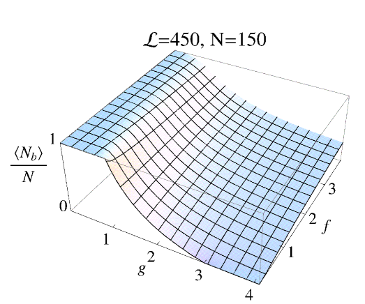
Figure 1: The boson fraction expectation value $\langle N_{b}\rangle/N$ as a function of the coupling parameters $f$, $g$, as given by (32). The results shown are for a system of ${\cal L}=450$ momentum pair states and ${N}=150$ pairs, giving the filling fraction as $x=1/3$. The boson fraction expectation value shows smooth variation between the BCS ($\langle N_{b}\rangle/N=0$) and BEC ($\langle N_{b}\rangle/N=1$) extremes.

3.2 Two-point correlation functions

• We first determine the off-diagonal two-point correlation function for $s_{m}^{\dagger}b$

  $$F(\{\lambda\},s_{m}^{\dagger}b,\{\lambda\})=\langle\phi(\{\lambda\})|s_{m}^{\dagger}b|\phi(\{\lambda\})\rangle.$$

The commutation relation between operators $b$ and ${\cal C}(\lambda)$, viz.

$$[b,{\cal C}(\lambda)]={2z_{b}\over\lambda}$$

allows us to commute the bosonic operator with all ${\cal C}(\lambda_{j})$. Considering that $b|0\rangle=0$ we obtain

$$F(\{\lambda\},s_{m}^{\dagger}b,\{\lambda\}) = \sum_{j=1}^{N}{2z_{b}\over\lambda_{j}}\langle\phi(\{\lambda\})|s_{m}^{\dagger}\prod_{k\neq j}^{N}{\cal C}(\lambda_{k})|0\rangle$$ (33)

$$= \langle\phi(\{\lambda\})|\phi(\{\lambda\})\rangle-\langle\phi(\{\lambda\})|\phi(\{\lambda\})\rangle$$

$$\mbox{~{}~{}~{}}+\lim_{v\rightarrow z_{m}^{2}}{v-z_{m}^{2}\over z_{m}}\sum_{j=1}^{N}{2z_{b}\over\lambda_{j}}\langle\phi(\{\lambda\})|{\cal C}(v)\prod_{k\neq j}^{N}{\cal C}(\lambda_{k})|0\rangle$$

$$= \mbox{det}{\widetilde{G}}(\{\lambda\})-\mbox{det}\left({\widetilde{G}}(\{\lambda\})-{\widetilde{M}}_{m}(\{\lambda\})\right)$$

with the elements of the rank-one matrix ${\widetilde{M}}_{m}$ as

$$\left({\widetilde{M}}_{m}(\{\lambda\})\right)_{ij}={2z_{b}z_{m}(\lambda_{j}-z_{m}^{2})\over\lambda_{j}(\lambda_{i}-z_{m}^{2})^{2}}.$$

The canonical two-point function with the definition

$$\langle bs^{\dagger}_{n}\rangle={\langle\phi(\{\lambda\})|s_{n}^{\dagger}b|\phi(\{\lambda\})\rangle\over\langle\phi(\{\lambda\})|\phi(\{\lambda\})\rangle}.$$

is expressible, using (33), as

$$\langle bs^{\dagger}_{n}\rangle=1-{\mbox{det}\left({\widetilde{G}}(\{\lambda\})-{\widetilde{M}}_{n}(\{\lambda\})\right)\over\mbox{det}\left({\widetilde{G}}(\{\lambda\})\right)}.$$ (34)

Fig. 2 illustrates the behaviour of the ground-state two-point function $\langle bs_{n}^{\dagger}\rangle$ as a function of the coupling parameters $f,g$. In all instances there is a rapid decrease in the fluctuations as $f\rightarrow 0$, but they appear smooth nonetheless for $f,g>0$. Fig. 3 shows the scaling behaviour of these two-point functions. These results indicate that, for a fixed value of $g$, we may write

$$\langle bs_{n}^{\dagger}\rangle=\phi_{n}(x,f)\theta_{n}(f/{\cal L})$$

where $\phi_{n}(x,f)$ is finite and $\theta_{n}(f/{\cal L})$ has the property that $\theta_{n}(0)=0$. For the thermodynamic limit $N,\,{\cal L}\rightarrow\infty$ with $x=N/{\cal L}$ we conclude that $\langle bs_{n}^{\dagger}\rangle\rightarrow 0$, which is one of the main assumptions underlying the mean-field treatment discussed in the Appendix.

$\begin{array}[]{cc}\epsfbox{ cf_M50_s1.eps }&\epsfbox{cf_M50_s100.eps}\\[11.38092pt] \mbox{\bf(a)}&\mbox{\bf(b)}\\[11.38092pt] \epsfbox{cf_M150_s1.eps}&\epsfbox{cf_M150_s100.eps}\\[11.38092pt] \mbox{\bf(c)}&\mbox{\bf(d)}\end{array}$

Figure 2: Ground-state two-point correlation function $\langle bs_{n}^{\dagger}\rangle$ (34), as a function of the coupling parameters $f$ and $g$. These two pinjt functions represent the boson-Cooper pair quantum fluctuations in finite systems where $\langle b\rangle=\langle s_{n}^{\dagger}\rangle=0$, Here ${\cal L}=100$ and the distribution of the momenta is $|{\mathbf{k}}|=\sqrt{2n}$. The insets correspond to the cases (a) $N=50$, $n=1$; (b) $N=50$, $n=100$; (c) $N=150$; $n=1$; (d) $N=150$, $n=100$. For intermediate values $1<n<100$ we have found that $\langle bs_{n}^{\dagger}\rangle$ has the same generic profile. It is apparent that increasing $N$ is associated with increasing fluctuations.

$\begin{array}[]{cc}\epsfbox{bsL-f.eps}&\epsfbox{bsL-frootL.eps}\\[11.38092pt] \mbox{\bf(a)}&\mbox{\bf(b)}\\[11.38092pt] \epsfbox{bshL-frootL.eps}&\epsfbox{fbs1-frootL.eps}\\[11.38092pt] \mbox{\bf(c)}&\mbox{\bf(d)}\end{array}$

Figure 3: Relationships between the boson-Cooper pair quantum fluctuations $\langle bs_{n}^{\dagger}\rangle$ and the rescaled coupling parameter $f/\sqrt{{\cal L}}$ with $g=100$, for different pairs of $({\cal L},N)$. The momentum distribution has been rescaled as $|{\mathbf{k}}|=\sqrt{2n/\cal L}$. Inset (a) shows the fluctuations for the case $n=\cal L$ as functions of $f$. Here there are nine distinguishable curves corresponding to the choices of $({\cal L},N)$ where ${\cal L}=100,200,330$ and $N=50,100,150$. The remaining insets for (b) $n=\cal L$, (c) $n={\cal L}/2$, (d) $n=1$ illustrate that, with the inclusion of scaling factors, the pair quantum fluctuations can be expressed by functions of the variable $f/\sqrt{\cal L}$. These cases also display data for the nine choices of $({\cal L},N)$, which is seen to fall on a single curve. The scaled fluctuations go to zero as $f/\sqrt{\cal L}\rightarrow 0$. This indicates that the fluctuations vanish in the thermodynamic limit $N,\,{\cal L}\rightarrow\infty$, with $x=N/{\cal L}$ finite.

For the remainder of this subsection we calculate three more cases of two-point correlation functions. Although we will not numerically evaluate these examples, the formulae are included for completeness.

• Here we calculate the two-point correlation function for $s^{\dagger}_{m}s_{n}$

  $$F(\{\lambda\},s_{m}^{\dagger}s_{n},\{\lambda\})=\langle\phi(\{\lambda\})|s_{m}^{\dagger}s_{n}|\phi(\{\lambda\})\rangle$$

Operating $s_{n}$ on the state $|\phi(\{\lambda\})\rangle$, we have

$$s_{n}|\phi(\{\lambda\}_{N})\rangle=s_{n}\prod_{\beta=1}^{N}{\cal C}(\lambda_{\beta})|0\rangle=s_{n}\prod_{\beta=1}^{N}\left(\widetilde{\cal C}_{n}(\lambda_{\beta})+A_{n}^{\beta}s^{\dagger}_{n}\right)|0\rangle,$$

where

$$\widetilde{\cal C}_{n}(\lambda_{\beta})={2z_{b}b^{\dagger}\over\lambda_{\beta}}+\sum_{l\neq n}^{N}{z_{l}s^{\dagger}_{l}\over\lambda_{\beta}-z_{l}^{2}},\quad\quad A_{n}^{\beta}={z_{n}\over\lambda_{\beta}-z_{n}^{2}}.$$

Bearing in mind that $(s^{\dagger}_{n})^{2}=0,\,\,s_{n}|0\rangle=0$, we find that the non-zero terms in the above relation combine to give

$$s_{n}|\phi(\{\lambda\})\rangle = \sum_{\beta=1}^{N}A_{n}^{\beta}\prod_{\alpha\neq\beta}^{N}\widetilde{\cal C}_{n}(\lambda_{\beta})|0\rangle$$ (35)

$$= \sum_{\beta=1}^{N}A_{n}^{\beta}\prod_{\alpha\neq\beta}^{N}\left({\cal C}(\lambda_{\alpha})-A_{n}^{\alpha}s^{\dagger}_{n}\right)|0\rangle$$

$$= \sum_{\beta=1}^{N}A_{n}^{\beta}\prod_{\alpha\neq\beta}^{N}{\cal C}(\lambda_{\alpha})|0\rangle-2\sum_{\beta=1}^{N}\sum_{\alpha<\beta}^{N}A_{n}^{\alpha}A_{n}^{\beta}s^{\dagger}_{n}\prod_{\gamma\neq\alpha,\beta}^{N}{\cal C}(\lambda_{\gamma})|0\rangle.$$

With the aid of (35), the two-point function reduces to

$$F(\{\lambda\},s^{\dagger}_{m}s_{n},\{\lambda\}) = \sum_{\beta=1}^{N}A_{n}^{\beta}\langle\phi(\{\lambda\})|s^{\dagger}_{m}\prod_{\alpha\neq\beta}^{N}{\cal C}(\lambda_{\alpha})|0\rangle$$

$$\mbox{}\quad-2\sum_{\beta=1}^{N}\sum_{\alpha<\beta}^{N}A_{n}^{\alpha}A_{n}^{\beta}\langle\phi(\{\lambda\})|s^{\dagger}_{m}s^{\dagger}_{n}\prod_{\gamma\neq\alpha,\beta}^{N}{\cal C}(\lambda_{\gamma})|0\rangle.$$

Now the two-point function for $s^{\dagger}_{m}s_{n}$ has been simplified to sums of one-point functions of $s^{\dagger}_{m}$ and two-point functions of $s^{\dagger}_{m}s^{\dagger}_{n}$. For the first term, we have

$$\sum_{\beta=1}^{N}A_{n}^{\beta}\langle\phi(\{\lambda\})|s^{\dagger}_{m}\prod_{\alpha\neq\beta}^{N}{\cal C}(\lambda_{\alpha})|0\rangle=\sum_{\beta=1}^{N}\left[A_{n}^{\beta}(\lambda_{\beta}-z_{m}^{2})\right]\mbox{det}{\widetilde{T}}_{m}^{\beta}(\{\lambda\}),$$

where

$$\left({\widetilde{T}}_{m}^{\beta}(\{\lambda\})\right)_{ij} = \left({\widetilde{G}}(\{\lambda\})\right)_{ij},\quad j\neq\beta,$$

$$\left({\widetilde{T}}_{m}^{\beta}(\{\lambda\})\right)_{i\beta} = {z_{m}\over(\lambda_{i}-z_{m}^{2})^{2}}.$$

For the second term, we have

$$2\sum_{\beta=1}^{N}\sum_{\alpha<\beta}^{N}A_{n}^{\alpha}A_{n}^{\beta}\langle\phi\{\lambda\})|s^{\dagger}_{m}s^{\dagger}_{n}\prod_{\gamma\neq\alpha,\beta}^{N}{\cal C}(\lambda_{\gamma})|0\rangle$$

$$=\lim_{u\rightarrow z_{m}^{2}}\lim_{v\rightarrow z_{n}^{2}}{(u-z_{m}^{2})(v-z_{n}^{2})\over z_{m}z_{n}}\sum_{\beta=1}^{N}\sum_{\alpha<\beta}^{N}2A_{n}^{\alpha}A_{n}^{\beta}\langle\phi\{\lambda\})|{\cal C}(u){\cal C}(v)\prod_{\gamma\neq\alpha,\beta}^{N}{\cal C}(\lambda_{\gamma})|0\rangle$$

$$=\sum_{\beta=1}^{N}\left(\left[A_{n}^{\beta}(\lambda_{\beta}-z_{m}^{2})\right]\sum_{\alpha<\beta}^{N}K_{mn}^{\alpha\beta}\mbox{det}({\widetilde{T}}_{mn}^{\alpha\beta}(\{\lambda\}))\right)$$

with

$$({\widetilde{T}}_{mn}^{\alpha\beta}(\{\lambda\}))_{ij}=\left({\widetilde{G}}(\{\lambda\})\right)_{ij},\qquad j\neq\alpha,\beta,$$

$$({\widetilde{T}}_{mn}^{\alpha\beta}(\{\lambda\}))_{i\alpha}={z_{n}\over(\lambda_{i}-z_{n}^{2})^{2}},\quad\quad({\widetilde{T}}_{mn}^{\alpha\beta}(\{\lambda\}))_{i\beta}={z_{m}\over(\lambda_{i}-z_{m}^{2})^{2}},$$

$$K_{mn}^{\alpha\beta}={2z_{n}(\lambda_{\alpha}-z_{m}^{2})(\lambda_{\beta}-z_{n}^{2})\over(\lambda_{\alpha}-\lambda_{\beta})(z^{2}_{m}-z^{2}_{n})}.$$

We can therefore express this two-point function as

$$F(\{\lambda\},s^{\dagger}_{m}s_{n},\{\lambda\})$$

$$\ \ =\sum_{\beta=1}^{N}\left[A_{n}^{\beta}(\lambda_{\beta}-z_{m}^{2})\right]\left(\mbox{det}{\widetilde{T}}_{m}^{\beta}(\{\lambda\})-\sum_{\alpha<\beta}K_{mn}^{\alpha\beta}\mbox{det}({\widetilde{T}}_{mn}^{\alpha\beta}(\{\lambda\}))\right).$$

Writing the columns of the matrices ${\widetilde{T}}_{m}^{\beta}$ and ${\widetilde{T}}_{mn}^{\alpha\beta}$ in vector notation, we have

$$\mbox{det}({\widetilde{T}}_{m}^{\beta}) = \mbox{det}\left(\vec{G}_{1},\ldots,\vec{G}_{\beta-1},\vec{W}_{m},\vec{G}_{\beta+1},\ldots,\vec{G}_{N}\right),$$

$$\mbox{det}({\widetilde{T}}_{mn}^{\alpha\beta}) = \mbox{det}\left(\vec{G}_{1},\ldots,\vec{G}_{\alpha-1},\vec{W}_{n},\vec{G}_{\alpha+1}\ldots\,\vec{G}_{\beta-1},\vec{W}_{m},\vec{G}_{\beta+1},\ldots,\vec{G}_{N}\right),$$

where $\vec{G}_{j}$, $j=1,\ldots,N$ denotes the $N$-dimensional vector with entries $(\vec{G}_{j})_{i}={\widetilde{G}}_{ij}$ and $\vec{W}_{x}$ $(x=m,n)$ denotes the $N$-dimensional vector with entries

$$(\vec{W}_{x})_{i}={z_{x}\over(\lambda_{i}-z_{x}^{2})^{2}}.$$

Note that we have refrained from detailing the explicit dependence on $\{\lambda\}$ in the above expression, and hope it is still clear to the reader. We focus our attention on simplifying the expression

$$\mbox{det}{\widetilde{T}}_{m}^{\beta}-\sum_{\alpha<\beta}K_{mn}^{\alpha\beta}\mbox{det}{\widetilde{T}}_{mn}^{\alpha\beta}$$

for each permissible $\beta.$ Using properties of determinants, it is possible to establish that

$$\mbox{det}{\widetilde{T}}_{m}^{\beta}-\sum_{\alpha<\beta}K_{mn}^{\alpha\beta}\mbox{det}{\widetilde{T}}_{mn}^{\alpha\beta}=\mbox{det}{\widetilde{X}}_{mn}^{\beta}$$

where

$$\left({\widetilde{X}}_{mn}^{\beta}\right)_{ij} = {\widetilde{G}}_{ij}-K_{mn}^{j\beta}{z_{n}\over(\lambda_{i}-z_{n}^{2})^{2}},\ \ j<\beta,$$

$$\left({\widetilde{X}}_{mn}^{\beta}\right)_{i\beta} = {z_{m}\over(\lambda_{i}-z_{m}^{2})^{2}},$$

$$\left({\widetilde{X}}_{mn}^{\beta}\right)_{ij} = {\widetilde{G}}_{ij},\ \ j>\beta.$$

Therefore, the two-point function simplifies to

$$F(\{\lambda\},s^{\dagger}_{m}s_{n},\{\lambda\}) = \sum_{\beta=1}^{N}\left[{z_{n}(\lambda_{\beta}-z_{m}^{2})\over\lambda_{\beta}-z_{n}^{2}}\right]\mbox{det}{\widetilde{X}}_{mn}^{\beta}(\{\lambda\})$$

We remark that the above procedure for reducing the double sum of determinants to a single sum leads to a more compact expression compared to the analogous result in [15].

• Two-point function of ${N}_{m}{N}_{n}$

Now we consider the two-point function of ${N}_{m}{N}_{n}$

$$F(\{\lambda\},{N}_{m}{N}_{n},\{\lambda\})=\langle\phi(\{\lambda\})|{N}_{m}{N}_{n}\prod_{i=1}^{N}{\cal C}(\lambda_{i})|0\rangle.$$

Commuting the number operators by using the commutation relation (30), we derive the correlation function as follows:

$$F(\{\lambda\},{N}_{m}{N}_{n},\{\lambda\}) = \langle\phi(\{\lambda\})|{N}_{m}{N}_{n}\prod_{i=1}^{N}{\cal C}(\lambda_{i})|0\rangle$$

$$= \sum_{\beta=1}^{N}{z_{m}\over\lambda_{\beta}-z_{m}^{2}}\langle\phi(\{\lambda\})|{N}_{n}s_{m}^{\dagger}\prod_{\alpha\neq\beta}^{N}{\cal C}(\lambda_{\alpha})|0\rangle$$

$$= \sum_{\beta=1}^{N}{z_{m}\over\lambda_{\beta}-z_{m}^{2}}\sum_{\alpha\neq\beta}^{N}{z_{n}\over\lambda_{\alpha}-z_{n}^{2}}\langle\phi(\{\lambda\})|s_{m}^{\dagger}s_{n}^{\dagger}\prod_{\gamma\neq\alpha,\beta}^{N}{\cal C}(\lambda_{\gamma})|0\rangle$$

$$= \sum_{\beta=1}^{N}\sum_{\alpha\neq\beta}^{N}J_{mn}^{\alpha\beta}\mbox{det}({\widetilde{T}}_{mn}^{\alpha\beta})$$

$$= \sum_{\beta=1}^{N}\sum_{\alpha<\beta}^{N}(J_{mn}^{\alpha\beta}-J_{mn}^{\beta\alpha})\mbox{det}({\widetilde{T}}_{mn}^{\alpha\beta})$$

$$= \sum_{\beta=2}^{N}\left[\mbox{det}({\widetilde{T}}_{m}^{\beta})-\mbox{det}({\widetilde{T}}_{m}^{\beta})\right]+\sum_{\beta=1}^{N}\sum_{\alpha<\beta}^{N}(J_{mn}^{\alpha\beta}-J_{mn}^{\beta\alpha})\mbox{det}({\widetilde{T}}_{mn}^{\alpha\beta}),$$

where

$$J_{mn}^{\alpha\beta}={z_{m}z_{n}(\lambda_{\alpha}-z_{m}^{2})(\lambda_{\beta}-z_{n}^{2})\over(z^{2}_{m}-z^{2}_{n})(\lambda_{\alpha}-\lambda_{\beta})}.$$

At this stage it is worth pointing out the obvious fact that in the second term in the last line of calculation above, the summation never sees the $\beta=1$ term, so we can proceed by writing

$$F(\{\lambda\},{N}_{m}{N}_{n},\{\lambda\}) = \sum_{\beta=2}^{N}\left[\mbox{det}({\widetilde{T}}_{m}^{\beta})+\sum_{\alpha<\beta}^{N}(J_{mn}^{\alpha\beta}-J_{mn}^{\beta\alpha})\mbox{det}({\widetilde{T}}_{mn}^{\alpha\beta})\right]-\sum_{\beta=2}^{N}\mbox{det}({\widetilde{T}}_{m}^{\beta}).$$

For each $\beta$, using similar techniques as before, the expression in square brackets above can be simplified to a single determinant, namely

$$\mbox{det}({\widetilde{T}}_{m}^{\beta})+\sum_{\alpha<\beta}^{N}(J_{mn}^{\alpha\beta}-J_{mn}^{\beta\alpha})\mbox{det}({\widetilde{T}}_{mn}^{\alpha\beta})=\mbox{det}({\widetilde{Y}}_{mn}^{\beta}),$$

where the matrix elements are

$$\left({\widetilde{Y}}_{mn}^{\beta}\right)_{ij} = {\widetilde{G}}_{ij}+(J_{mn}^{j\beta}-J_{mn}^{\beta j}){z_{n}\over(\lambda_{i}-z_{n}^{2})^{2}},\ \ j<\beta,$$

$$\left({\widetilde{Y}}_{mn}^{\beta}\right)_{i\beta} = {z_{m}\over(\lambda_{i}-z_{m}^{2})^{2}},$$

$$\left({\widetilde{Y}}_{mn}^{\beta}\right)_{ij} = {\widetilde{G}}_{ij},\ \ j>\beta.$$

Once again using familiar properties of the determinant, we may also simplify

$$\sum_{\beta=2}^{N}\mbox{det}({\widetilde{T}}_{m}^{\beta})=\mbox{det}(A_{m}),$$

where the matrix $A_{m}$ has elements given by

$$(A_{m})_{i1} = {\widetilde{G}}_{i1},$$

$$(A_{m})_{ij} = {\widetilde{G}}_{ij}-{\widetilde{G}}_{ij+1},\ \ 1<j<N,$$

$$(A_{m})_{iN} = {z_{m}\over(\lambda_{i}-z_{m}^{2})^{2}}.$$

In the above we have supressed the explicit dependency on $\{\lambda\}$ in each of the expressions, as it should be clear. Therefore the two-point function can be expressed as a sum of $N$ determinants

$$F(\{\lambda\},{N}_{m}{N}_{n},\{\lambda\})=\sum_{\beta=2}^{N}\mbox{det}({\widetilde{Y}}_{mn}^{\beta}(\{\lambda\}))-\mbox{det}(A_{m}(\{\lambda\})).$$

• Two-point function of $N_{b}{N}_{m}$

To compute the two-point function

$$F(\{\lambda\},N_{b}{N}_{m},\{\lambda\})=\langle\phi(\{\lambda\})|N_{b}{N}_{m}\prod_{i=1}^{N}{\cal C}(\lambda_{i})|0\rangle,$$

we need to use commutation relations both (29) and (30). The result is given by

$$F(\{\lambda\},N_{b}{N}_{m},\{\lambda\})=\sum_{\beta=1}^{N}{z_{m}\over\lambda_{\beta}-z_{m}^{2}}\sum_{\alpha\neq\beta}^{N}{2z_{b}\over\lambda_{\alpha}}\langle\phi(\{\lambda\})|s_{m}^{\dagger}b^{\dagger}\prod_{\gamma\neq\alpha,\beta}^{N}{\cal C}(\lambda_{\gamma})|0\rangle$$

$$=\lim_{u\rightarrow z_{m}^{2}}\sum_{\beta=1}^{N}{u-z_{m}^{2}\over\lambda_{\beta}-z_{m}^{2}}\lim_{v\rightarrow 0}\sum_{\alpha\neq\beta}^{N}{v\over\lambda_{\alpha}}\langle\phi(\{\lambda\})|{\cal C}(u){\cal C}(v)\prod_{\gamma\neq\alpha,\beta}^{N}{\cal C}(\lambda_{\gamma})|0\rangle$$

$$=\sum_{\beta=1}^{N}\sum_{\alpha\neq\beta}^{N}\widetilde{J}_{mn}^{\alpha\beta}\mbox{det}({\widetilde{D}}_{mn}^{\alpha\beta})$$

$$=\sum_{\beta=1}^{N}\sum_{\alpha<\beta}(\widetilde{J}_{mn}^{\alpha\beta}-\widetilde{J}_{mn}^{\beta\alpha})\mbox{det}({\widetilde{D}}_{mn}^{\alpha\beta})$$

where

$$\widetilde{J}_{mn}^{\alpha\beta}={2z_{b}\lambda_{\beta}(\lambda_{\alpha}-z_{m}^{2})\over z_{m}(\lambda_{\alpha}-\lambda_{\beta})},$$

$$({\widetilde{D}}_{mn}^{\alpha\beta})_{ij}={\widetilde{G}}_{ij}~{}~{}~{}(j\neq\alpha,\beta),~{}~{}~{}~{}~{}(\widetilde{D}_{mn}^{\alpha\beta})_{i\alpha}={2z_{b}\over\lambda_{j}^{2}},\quad\quad(\widetilde{D}_{mn}^{\alpha\beta})_{i\beta}={z_{m}\over(\lambda_{i}-z_{m}^{2})^{2}}.$$

Using similar techniques as before, we can reduce the above to a sum of $N$ determinants. Doing this leads to

$$F(\{\lambda\},{N}_{b}{N}_{m},\{\lambda\})\\ =\sum_{\beta=2}^{N}\mbox{det}({\widetilde{Z}}_{mn}^{\beta}(\{\lambda\}))-\mbox{det}(A_{m}(\{\lambda\}))$$

where the elements of ${\widetilde{Z}}^{\beta}_{mn}$ are given by

$$\left({\widetilde{Z}}_{mn}^{\beta}\right)_{ij} = {\widetilde{G}}_{ij}+2({\widetilde{J}}_{mn}^{j\beta}-{\widetilde{J}}_{mn}^{\beta j}){z_{b}\over\lambda_{i}^{2}},\ \ j<\beta,$$

$$\left({\widetilde{Z}}_{mn}^{\beta}\right)_{i\beta} = {z_{m}\over(\lambda_{i}-z_{m}^{2})^{2}},$$

$$\left({\widetilde{Z}}_{mn}^{\beta}\right)_{ij} = {\widetilde{G}}_{ij},\ \ j>\beta.$$

4 Conclusion

We have introduced a model that couples a $p+ip$-wave pairing BCS Hamiltonian to a bosonic degree of freedom, and studied its properties regarding the BEC-BCS crossover. For a restriction on the coupling parameters, the model was shown to be integrable and the exact solution was derived by the algebraic Bethe ansatz. We found that the ground-state roots of the Bethe ansatz equations have the property that they are the unique solution set such that all roots are real and negative. Using this result we reasoned that the ground-state wavefunction is topologically trivial, so the BEC-BCS crossover is smooth. This conclusion was supported by a study of the boson fraction expectation value, which was computed exactly in the Bethe ansatz framework. We also formulated expressions for a range of two-point correlation functions and used one particular example to study the boson-Cooper pair fluctuations. The range of correlation function expressions we have obtained provide ample scope for further studies along the lines of [10].

Acknowledgments C.D. and J.L. were funded through the Royal Society Travel Grants Scheme. C.D. acknowledges support through EPSRC grant EP/G039526/1. P.S.I. was supported by an Early Career Researcher Grant from The University of Queensland. J.L. and S.-Y.Z. received funding by the Australian Research Council through Discovery Project DP0663772. J.L. also acknowledges support through Discovery Project DP110101414.

5 Appendix - Mean-field theory

In the mean-field approach products of operators $A$ and $B$ are approximated by

$$AB\approx A\langle B\rangle+\langle A\rangle B-\langle A\rangle\langle B\rangle$$ (36)

where the notation $\langle\cdot\rangle$ stands for the expectation value. This approximation assumes that quantum fluctuations may be neglected. Formally, we define the fluctuations to be

$$\chi(A,B)=\left|\langle AB\rangle-\langle A\rangle\langle B\rangle\right|$$

such that within the mean-field approximation (36) we have

$$\chi(A,B)=0.$$

Applying (36) to (3) we obtain the mean-field Hamiltonian

$$H_{MF} = H_{0}+\left({K^{2}\over G}+\delta\right)N_{b}-{1\over 2G}\widetilde{\Delta}^{*}(GQ+Kb)-{1\over 2G}\widetilde{\Delta}(GQ^{\dagger}+Kb^{\dagger})$$ (37)

$$\mbox{}+{1\over 4G}|\widetilde{\Delta}|^{2}-\nu(N-\langle N\rangle),$$

where $\Delta=2G\langle Q\rangle+2K\langle b\rangle$ is referred to as the gap. Since (37) does not commute with ${N}$ the Lagrange multiplier $\nu$, the chemical potential, has been introduced in order to tune the expectation value $\langle{N}\rangle$.

We take the following form for the mean-field variational ground state

$$|\Psi\rangle=|\alpha\rangle\otimes|\psi_{1}\rangle\otimes|\psi_{2}\rangle\otimes....\otimes|\psi_{\cal L}\rangle,$$

where $|\alpha\rangle$ is the coherent state such that $b|\alpha\rangle=\alpha|\alpha\rangle$ with $\alpha=|\alpha|e^{i\phi}\in{\mathbb{C}}$, and $|\psi_{j}\rangle$ are local states related to the pairing operators

$$|\psi_{j}\rangle = (u_{j}I+v_{j}s^{\dagger}_{j})|0_{j}\rangle$$

with $|0_{j}\rangle$ the vacuum state of the momentum pair space labelled by $j$. Minimising the ground-state energy expectation value and imposing self-consistency of other operator expectation values leads to the following set of equations determining the values for $\alpha$, the gap $\Delta$, and the chemical potential $\nu$:

$$\alpha = {K\Delta\over 2(G\delta-G\nu+K^{2})},$$ (38)

$${\delta-\nu\over G\delta-G\nu+K^{2}} = \sum_{j=1}^{\cal L}{z_{j}^{2}\over\sqrt{(z_{j}^{2}-\nu)^{2}+z_{j}^{2}|\Delta|^{2}}},$$ (39)

$$2{N}-{\cal L}-{K\Delta^{2}\over 2(G\delta-G\nu+K^{2})^{2}}+{\delta-\nu\over G\delta-G\nu+K^{2}}$$

$$\qquad\qquad\qquad\quad=\,\nu\sum_{j=1}^{\cal L}{1\over\sqrt{(z_{j}^{2}-\nu)^{2}+z_{j}^{2}|\Delta|^{2}}}.$$ (40)

The ground state energy assumes the form

$$E=\nu|\alpha|^{2}+{1\over 2}\sum_{j=1}^{\cal L}z_{j}^{2}\left(1-{2z_{j}^{2}+|\Delta|^{2}-2\nu\over 2\sqrt{(z_{j}^{2}-\nu)^{2}+z_{j}^{2}|\Delta|^{2}}}\right)$$ (41)

and we also find

$$|u_{j}|^{2} = {1\over 2}\left(1+{z_{j}^{2}-\nu\over\sqrt{(z_{j}^{2}-\nu)^{2}+z_{j}^{2}|\Delta|^{2}}}\right),$$

$$|v_{j}|^{2} = {1\over 2}\left(1-{z_{j}^{2}-\nu\over\sqrt{(z_{j}^{2}-\nu)^{2}+z_{j}^{2}|\Delta|^{2}}}\right)=\langle{N}_{j}\rangle.$$

Let $\nu^{2}=ab$ and $2\nu-|\Delta|^{2}=a+b$. It can be verified that taking the continuum limit for (39)-(41) with the substitution (5) reproduces equations (22)-(24). Moreover when (5) holds, (38)-(40) lead to the result

$${\langle N_{b}\rangle\over N}={|\alpha|^{2}\over N}={f^{2}|\Delta|^{2}\over 16x\nu}=1-{1\over 2x}+{1\over 2x}\int^{\omega}_{0}d\varepsilon\,{\rho(\varepsilon)(\varepsilon+\sqrt{ab})\over R(\varepsilon)}.$$

This quantity is a smooth function for $f,g>0$, which can be shown by using the fact that $a,b<0$. It displays discontinuous behaviour (in the first derivative) only in the non-interacting limit $f\rightarrow 0$ when $g=1$ or $g^{-1}=1-2x$, which is due to level crossing. These correspond to the transition points of Table 2, and are visible in Fig. 1. The smoothness of the boson fraction expectation value for the interacting system in the thermodynamic limit is consistent with the absence of a phase transition between the BCS and BEC extremes.

References

• [1] C.A. Regal, M. Greiner, and D.S. Jin, Phys. Rev. Lett. 92, 040403 (2004); V. Gurarie and L. Radzihovsky, Ann. Phys. 322, 2 (2007); I. Bloch, J. Dalibard and W. Zwerger, Rev. Mod. Phys. 80, 885 (2008); K. Levin, Q. Chen, C.-C. Chien, and Y. He, Ann. Phys. 325, 233 (2010).
• [2] M. Holland, S.J.J.F. Kokkelmans, M.L. Chiofalo and R. Walser, Phys. Rev. Lett. 87, 120406 (2001); Y. Ohashi and A. Griffin, Phys. Rev. Lett. 89, 130402 (2002).
• [3] Y. Ohashi, Phys. Rev. Lett. 94, 050403 (2005); V. Gurarie, L. Radzihovsky, and A.V. Andreev, Phys. Rev. Lett. 94, 230403 (2005); C.-H. Cheng and S.-K. Yip, Phys. Rev. Lett. 95, 070404 (2005).
• [4] J.P. Gaebler, J.T. Stewart, J.L. Bohn, and D.S. Jin, Phys. Rev. Lett. 98, 200403 (2007).
• [5] C. Nayak, S.H. Simon, A. Stern, M. Freedman, and S. Das Sarma, Rev. Mod. Phys. 80, 1083 (2008); C. Zhang, S. Tewari, R.M. Lutchyn, S. Das Sarma, Phys. Rev. Lett. 101, 160401 (2008); M. Sato, Y. Takahashi, S. Fujimoto, Phys. Rev. Lett. 103, 020401 (2009); N.R. Cooper and G.V. Shlyapnikov, Phys. Rev. Lett. 103, 155302 (2009); R. Roy, Phys. Rev. Lett. 105, 186401 (2010).
• [6] N. Read and D. Green, Phys. Rev. B 61, 10267 (2000).
• [7] R.W. Richardson, Phys. Lett. 3, 277 (1963).
• [8] J. von Delft and D.C. Ralph, Phys. Rep. 345, 61 (2001).
• [9] M.C. Cambiaggio, A.M.F. Rivas, and M. Saraceno, Nucl. Phys. A 624, 157 (1997); L. Amico, G. Falci, and R. Fazio, J. Phys. A: Math. Gen. 34, 6425 (2001); J. von Delft and R. Poghossian, Phys. Rev. B 66, 134502 (2002); J. Links, H.-Q. Zhou, R.H. McKenzie, and M.D. Gould, J. Phys. A: Math. Gen. 36, R63 (2003); A.A. Ovchinnikov, Nucl. Phys. B 703, 363 (2003); J. Dukelsky, S. Pittel, and G. Sierra, Rev. Mod. Phys. 76, 643 (2004).
• [10] L. Amico and A. Osterloh, Phys. Rev. Lett. 88, 127003 (2002); C. Dunning, J. Links, and H.-Q. Zhou, Phys. Rev. Lett. 94, 227002 (2005); A. Faribault, P. Calabrese, and J.-S. Caux, Phys. Rev. B 77, 064503 (2008); A. Faribault, P. Calabrese, and J.-S. Caux, J. Stat. Mech.: Theor. Exp., P03018 (2009); A. Faribault, P. Calabrese, and J.-S. Caux, J. Math. Phys. 50, 095212 (2009); A. Faribault, P. Calabrese, and J.-S. Caux, Phys. Rev. B 81, 174507 (2010).
• [11] J. Dukelsky, G.G. Dussel, C. Esebbag, and S. Pittel, Phys. Rev. Lett. 93, 050403 (2004); E.A. Yuzbashyan, V.B. Kuznetsov, and B.L. Altshuler, Phys. Rev. B 72, 144524 (2005); K.E. Hibberd, C. Dunning, and J. Links, Nucl. Phys. B 748, 458 (2006); A.P. Itin, A.A. Vasiliev, G. Krishna, and S. Watanabe, Physica D 232, 108 (2007).
• [12] M. Gaudin, J. Phys. France 37, 1087 (1976); O. Tsyplyatyev, J. von Delft, and D. Loss, Phys. Rev. B 82, 092203 (2010).
• [13] M. Ibanez, J. Links, G. Sierra, and S.-Y, Zhao, Phys. Rev. B 79, 180501(R) (2009).
• [14] T. Skrypnyk, J. Phys. A: Math. Theor. 42, 472004 (2009).
• [15] C. Dunning, M. Ibanez, J. Links, G. Sierra, and S.-Y. Zhao, J. Stat. Mech. P08025 (2010).
• [16] S.M.A. Rombouts, J. Dukelsky, and G. Ortiz, Phys. Rev B 82, 224510 (2010).
• [17] L.D. Faddeev, E.K. Sklyanin, and L.A. Takhtajan, Theor. Math. Phys. 40, 688 (1979).
• [18] A. Kundu, SIGMA 3, 040 (2007).
• [19] N.A. Slavnov, Theor. Math. Phys. 79, 502 (1989).
• [20] G. E. Astrakharchik, J. Boronat, J. Casulleras, and S. Giorgini, Phys. Rev. Lett. 95, 230405 (2005).