Structural and dynamical properties of nanoconfined supercooled water

Bulk water presents a large number of crystalline and amorphous ices. Hydrophobic nanoconfinement is known to affect the tendency of water to form ice and to reduce the melting temperature. However, a systematic study of the ice phases in nanoconfinement is hampered by the computational cost of simulations at very low temperatures. Here we develop a coarse-grained model for a water monolayer in hydrophobic nanoconfinement and study the formation of ice by Mote Carlo simulations. We find two ice phases: low-density-crystal ice at low pressure and high-density hexatic ice at high pressure, an intermediate phase between liquid and high-density-crystal ice.

1 Introduction

Water phase diagram is very complex when compared to other liquids. For example, water is a polymorph with an unusually large number of solid phases (crystalline and amorphous ices): more than 20 with the last phase discoverered in 2009 [12]. Formation of ice in confined systems is a relevant subject in nanocience and biology, in areas like cryopreservation of food and human tissues or cells. Due to the property of water to expand when the liquid transforms into ice, the formation of ice in confinement can drammatically damage or destroy the confining structure. Therefore, it is important to understand the properties of ice in nanoconfinement, especially for hydrated systems at low temperature where water is highly confined, as for example in biological cells or on the surface of proteins at low hydration level [7, 9].

Simulations can help to answer open questions in this fields, but they are hampered by the large computational costs of calculations for large systems at low temperature with detailed models of water. With the aim of developing a model that preserve essential properties of water and is also computationally efficient, here we perform Monte Carlo simulations of a coarse-grained model of water. In its original formulation the model allows for very efficient simulation studies. On the other hand, it has a simple hamiltonian that allows for theoretical studies [5, 15], but does not allow the study of structural properties because the positions of water molecules are coarse-grained. Here, we extend the model, introducing the coordinates of the molecules $\vec{r}_{i}$ to perform the structural analysis. We study the phase diagram and, in particular, how the hydrophobic nanoconfinement affects the ice formation for a water monolayer. We find two forms of ice and we characterize their structure.

This work is organized as follows: we introduce the Model in the first section and give details about the Monte Carlo method in the second section; we present the results in the third section, discussing the structural and dynamical properties; we make our conclusions in the final section.

1.1 The Model

We consider a water monolayer confined between two hydrophobic plates at separation $h\simeq 1nm$. The hydrophobic interaction with the plates is schematically represented as purely repulsive. By molecular dynamics simulations of a detailed model of water, it has been shown that a water monloayer under these conditions forms a two-dimensional ice with square symmetry [8, 19, 18]. Therefore, we adopt a square partition to coarse grain the confined water, divinding the total occupied volume $V$ into $N$ cells of square section and height $h$. Each cell has a volume $v=V/N$ and the coarse grain is made with the hypothesis that the system is homogenous and each cell contains one single water molecule.

We consider the case in which pressure $P$, temperature $T$ and number of molecules $N$ are fixed, and the total volume $V$ can vary. Therefore, the volume per molecule $v$, and the number density $\rho\equiv 1/v$, are functions of $P$ and $T$ at any fixed $N$.

The hamiltonian of the model has several water-water interaction terms. The first is the isotropic Van der Waals interaction, due to dispersive attractive forces and short-range repulsive interactions, represented by a Lennard-Jones potential:

$$\mathcal{H}_{\text{VW}}\equiv\sum_{i<j}\varepsilon\left[\left(\frac{r_{0}}{r_{ij}}\right)^{12}-\left(\frac{r_{0}}{r_{ij}}\right)^{6}\right]$$ (1)

Here $\varepsilon\equiv 5.8$ kJ/mol is the characteristic energy, $r_{0}\equiv 2.9$ Å is the diameter of the molecules and $r_{ij}$ the distance between two water molecules in the cells $i$ and $j$. In order to reduce the computational cost of the simulations, we introduce a cutoff distance at $r_{\rm cutoff}=2.5r_{0}$ and add a linear term that set to zero the potential at $r_{\rm cutoff}$.

Two neighbouring molecules can form a hydrogen bond when the OH—O distance is less than $r_{\rm max}-r_{\rm OH}=3.14$Å, and if ${\widehat{\rm OOH}}<30^{\rm o}$. To account for this interaction the model includes a term

$$\mathcal{H}_{\text{HB}}\equiv-JN_{\text{HB}}$$ (2)

where $J\equiv 2.9$ kJ/mol and $N_{\text{HB}}\equiv\sum_{\langle i,j\rangle}\beta_{ij}$ with $\beta_{ij}\equiv\delta_{\sigma_{ij},\sigma_{ji}}\Theta(r_{ij}-r_{\rm max})$, and $\Theta(x)\equiv 1$ if $x>0$, or $0$ otherwise. Each molecules $i$ has a bond indices $\sigma_{ij}\in\{0,1,\dots q-1\}$ for each nearest neighbor molecule $j$. The choice $q=180º/30º=6$ accounts correctly for the entropy loss associated with the formation of a hydrogen bond because by definition $\delta_{\sigma_{ij},\sigma_{ji}}\equiv 1$ if $\sigma_{ij}=\sigma_{ji}$, $\delta_{\sigma_{ij},\sigma_{ji}}\equiv 0$ otherwise. The notation $\langle i,j\rangle$ denotes that the sum is performed over nearest neighbors, implying that each molecule cannot form more than 4 bonds with its nearest neighbours.

When water molecules form a hydrogen bond network, the resulting configuration occupies more space than at close packing. This effect is included in the model as a volume increase per formed bond equal to $v_{\text{HB}}=0.5v_{0}$, correspondig to the average density increase between high density ices VI and VIII and low density (tetrahedral) ice Ih in bulk water [13, 14]. The total volume of the system is, therefore, $V=V_{0}+v_{\text{HB}}N_{\text{HB}}$, where $V_{0}$ is the volume when there are no hydrogen bonds.

As an effect of cooperativity, the O-O-O angle distribution becomes sharper at lower $T$, reducing the possible orientations of the molecules [15, 3, 6]. This cooperative term, resulting from three-body interactions, is accounted for by the term

$$\mathcal{H}_{\text{coop}}\equiv-J_{\sigma}\sum_{i}\sum_{(k,l)_{i}}\delta_{\sigma_{ik},\sigma_{il}}\leavevmode\nobreak\ ,$$ (3)

where $J_{\sigma}\equiv 0.29$ kJ/mol, and $(k,\ell)_{i}$ indicates each of the six different pairs of the four bond-indices $\sigma_{ij}$ of a molecule $i$. The effect of this term is to locally drive the molecules toward an ordered configuration.

In its original formulation the model is defined by coarse-graining the molecules coordinates $r_{ij}$ with the center of each cell. Furthermore, the effect of the cooperativity on the O-O-O angle distribution is taken into account in terms of the associated entrophy change, but not in terms of angular coordinates. Therefore, no detailed structural analysis is possible. To allow the calculation of the radial distribution function $g(r)$ and the angular distribution function $g(\theta)$, in the following subsection we extend the original model introducing a term that explicitly depends on these variables.

1.1.1 Extension of the model

The new Hamiltonian term is a three-body interaction that depends on the formation of hydrogen bonds between triads of molecules and their relative angles $\theta^{i}_{kl}$:

$$\mathcal{H}_{\theta}\equiv J_{\theta}\sum_{i}\sum_{\langle\langle k,l\rangle\rangle_{i}}\beta_{ik}\beta_{il}\Delta(\theta_{kl}^{i}),$$ (4)

where $J_{\theta}=0.5\varepsilon$. The sum is over all the neighbouring pairs of molecules $k$ and $l$ that are bonded to the molecule $i$, with the restriction that $k$ and $l$ must be second nearest neighbors to each other. The function $\Delta(\theta)$ is a smooth function of the angle between the centers of the three molecules with a minimum at $\pi/2$. We adopt this choice because molecular dynamics simualtions of a detailed water model show that, under the conditions considered here, a confined water monolayer forms a square crystal [8, 19]. We chose

$$\Delta(\theta)\equiv\frac{1}{2}\left[1-\cos(4\theta)\right],$$

which is a non-negative function in $[0,1]$ with minima at $\pi/2$ and $\pi$, and we approximate it with

$$\Delta(\theta)\simeq 4(\theta-\pi/2)^{2}$$ (5)

around $\theta^{i}_{jk}\simeq\pi/2$.

This value of $J_{\theta}$ is set to avoid the formation of bonds when the $\theta^{i}_{jk}\approx 60^{\circ}$, because

$$\mathcal{H}_{\theta}(\theta^{i}_{jk}=\pi/3)=\mathcal{H}_{\theta}(\theta^{i}_{jk}=2\pi/3)\simeq 4NJ_{\theta},$$

and

$$\mathcal{H}_{\theta}+\mathcal{H}_{\text{J}}\simeq 4NJ_{\theta}+2NJ=2N\varepsilon-N\varepsilon=N\varepsilon>0.$$

Therefore, the formation of hydrogen bonds is energetically unfavourable when $\theta^{i}_{jk}\approx 60^{\circ}$.

The total hamiltonian of the model is

$$\mathcal{H}\equiv\mathcal{H}_{\text{VW}}+\mathcal{H}_{\text{HB}}+\mathcal{H}_{\text{IM}}+\mathcal{H}_{\theta}.$$ (6)

1.2 Metropolis MC method

We perform MC simulations at constant number of molecules $N=900$ and fixed pressure $P$ and temperature $T$, allowing fluctuations of the volume $V$. One MC step consists in updating $5N+1$ variables: $N$ vectors $\vec{r}_{i}$ describing the position of molecules with respect to the center of their cell, $4N$ bondig indices $\sigma_{ij}$ and the total volume $V_{0}$. We adopt the Metropolis algorithm: we choose one of the $5N+1$ variables at random and attempt to change its state to a new random value. We accept the new state with probability $\exp[-\beta\Delta G]$ if $\Delta G>0$ and with probability 1 otherwise. Here $\beta\equiv 1/k_{B}T$, $k_{B}$ is the Boltzamann constant, $\Delta G\equiv G_{\rm new}-G_{\rm old}$ is the change in Gibbs free energy if the new state is accepted, and

$$G \equiv U+PV-TS$$

$$=\mathcal{H}+PV-Nk_{\text{B}}T\log(V).$$ (7)

For a bonding index $\sigma_{ij}$, the new state is choosen at random among the $q=6$ possible states. For each components of $\vec{r}_{ij}$, the new value is set to $r_{\alpha,\text{new}}=r_{\alpha,\text{old}}+\epsilon_{r}$, where $\epsilon_{r}\in[-\delta r,+\delta r]$ is a random number and $\alpha=x$, $y$ (we do not change the component $z$ and consider it as a coarse-grained variable). The volume is updated with a random change $V_{0}^{\text{new}}=V_{0}^{\text{old}}+\epsilon_{V}$ where $\epsilon_{V}\in[-\delta V,+\delta V]$ is a random number [10]. The parameters $\delta r$ and $\delta V$ are adapted in such a way to keep the acceptance ratio $\approx 40\%$ (adaptive step size algorithm) [16, 1].

At any $P$, we equilibrate the system from random configurations at high $T$ for $10^{5}\sim 10^{6}$ MC steps and calculate the thermodynamic averages over the following $10^{6}\sim 10^{7}$ MC steps. Keeping $P$ constant, we perform an annealing, i.e. we decrease the temperature $T$ a few K and, starting from the last configuration at the previous temperature, we use the same statistics for equilibration and calculation of the averages. To take into account the correlation of the data for the calculation of the error on the estimates, we perform blocking averages where the size of each block depends on $P$ and $T$ and is determined as twice the number $\tau$ of MC steps needed to have uncorrelated data. The number $\tau$ is estimated from the autocorrelation functions introduced in Section 4.

2 Results

2.1 Phase Diagram

The phase diagram of the model displays the liquid-gas first-order phase transition ending in a critical point (Fig.1). In the liquid phase we observe that at any $P<0.2$ GPa the density is non monotonic. The locus of temperatures of maximum density (TMD) follows a line in the $P$-$T$ phase diagram, reproducing one of the characteristc anomalies of water.

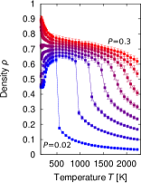
(a)

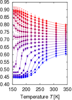
(b)

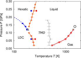
(c)

Figure 1: (a) Isobars for the confined water monolayer in the $\rho-T$ phase diagram display a discontinuity that marks the first-order liquid-gas phase transition ending in a critical point (at $P=0.16\pm 0.02$ GPa, $T=1500\pm 200$ K) and a density maximum for $P<0.20$ GPa. Isobars are for $P\in[0.02,0.3]$ GPa separated by $0.04$ GPa (from the bottom). (b) At low $T$ a sudden decrease in $\rho$ suggests the occurrence of another phase transition. As we discuss in the analysis, we associate this sudden change in $\rho$ to the first-order phase transition between the liquid and a low density crystal (LDC). Pressures are as in (a) but with a separation of $0.02$ GPa. (c) The $P-T$ phase diagram with gas-liquid coexistence line ending at the gas-liquid critical point (open circle) and the line of temperatures of maximum density (TMD). At low $T$ and low $P$, the liquid–LDC coexistence line merges, at about $P=0.11\pm 0.01$ GPa and $T=190\pm 20$ K (open triangle), with a line with positive slope corresponding to the liquid-hexatic phase transition, as described in the text. Full circles are the state points of the distribution functions in Fig.s 2,3.

At low $P$ and low $T$ we find a rapid decrease of density $\rho$. This is the consequence of formation of a large number of hydrogen bonds and the cooperative reorientation of the molecules into a crystal configuration. In the next section we caracterize this crystal as low-density crystal (LDC) with a square cell in its 2D projection.

At high $P$ and low $T$ our structural and dynamical analysis, presented in the next sections, show that the system “freezes” into a solid. However, the solid has no long-range translational order, but short-range translational order and quasi-long-range orientational order. This is, by definition, an “hexatic” phase, described by the theory of Kosterlitz, Thouless, Halperin, Nelson, and Young [2, 11] for crystallization in 2D systems. The theory tells us that the hexatic phase is intermediate between the crystal and the liquid phases and is separated by continuous phases transitions with both phases. This is consistent with the fact that we do not observe any discontinuity in the density at high $P$ and low $T$ (Fig. 1) and that our system is essentially in 2D because we coarse-grain the $z$-component of the molecules. The hexatic-liquid coexistence is characterized by the unbinding of disclinations, i.e. lines of defects at which rotational symmetry is violated. The crystal-hexatic coexistence is where occurs the unbinding of dislocations, i.e. particle-like topological defects. The associated crystal phase is characterized by the same orientational order of the hexatic phase, that is, as described in the next section, hexagonal (or close-packing) and has a higher density of the LDC. We therefore call it high-density crystal (HDC). Finally, the structural analysis allows us to estimate the coexistence line between the LDC and the hexatic phase and the triple point where liquid, hexatic and LDC phases coexist (Fig. 1).

It is interesting to observe that the phase diagram of our confined monolayer reproduces the change of slope of the “ice” line observed for bulk water. The slope is negative at low $P$ and is positive at high $P$. The ice phase at low $P$ is LDC characterized by hydrogen bonds at $90^{\circ}$. At high $P$ the solid phase is hexatic, where the number of hydrogen bonds is largely reduced and the water interaction is dominated by the Lennard-Jones potential, as in simple liquids.

2.2 Structural Properties

The radial distribution function

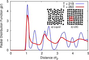
(a) Low pressure at $P=0.06$ GPa

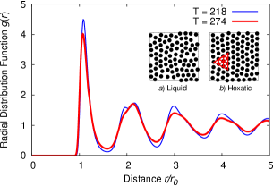
(b) High pressure at $P=0.24$ GPa

Figure 2: Radial Distribution Functions for the state points marked as coloured full circles in Fig.1. (a) At $P=0.06$ GPa and $T=246$ K (in the liquid phase) and $T=218$ K (in the LDC phase). Here and in the next panel, insets show a portion of typical configurations at the state points represented in the main panels. The $g(r)$ for the LDC has many peaks correspoding to the long-range translational order of the square crystal, while the $g(r)$ for the liquid near the coexistence shows precursors of the LDC structure. (b) At $P=0.24$ GPa and $T=274$ K (in the liquid phase) and $T=218$ K (in the hexatic phase). The liquid $g(r)$ has a shoulder in the second peak that splits into a small peak in the hexatic phase. The hexatic phase has liquid-like short-range translational order due to the presence of many disclinations, but crystal-like long-range orientational order, emphasized by links in the inset describing the hexatic phase.

To study the static properties of the system we calculate the radial distribution function (RDF) as

$$g(r)\equiv\frac{1}{\rho^{2}V}\sum_{i\neq j}\delta(r-r_{ij}).$$ (8)

The quantity $g(r)2\pi rdr$ is proportional to the probability of finding a molecule at a distance $r$ from a central one.

By crossing the ice-liquid lines of Fig.1c we can observe structural changes in the $g(r)$. At low $P$ (Fig.2a), we find a large change in $g(r)$ within a narrow range of $T$, marking the occurrence of the liquid-LDC first-order phase transition. The LDC is characyerized by square long-range translational order.

At high $P$ (Fig.2b), we observe a shoulder in the second peak of the $g(r)$ for the liquid. This shoulder develops into a small peak at lower $T$. This structural change has been characterized [17] as the liquid-hexatic second-order phase transition. This interpretation is consistent with the analysis of the typical configurations at the lower $T$, showing liquid-like short-range translational order and crystal-like long-range orientational (hexagonal) order. The hexatic phase is the precursor of the HDC close-packing crystal. The solid-like properties of this phase are confirmed by the analysis presented in the next section.

Finally, at low $T$ by increasing $P$ the structural analys allows us to locate the coexistence between the LDC and the hexatic phase. The transition is charcterized by a sharp change of $g(r)$ indicating a first-order phase transition between the LDC and the hexatic phase.

The angular distribution

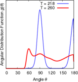
(a) Low pressure at $P=0.06$ GPa

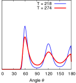
(b) High pressure at $P=0.24$ GPa

Figure 3: The angular distribution functions $g(\theta)$, calculated at the same state points as in Fig.2, emphasizes the long-range orientational order in the LDC and the hexatic phases.

To charcterize the structure, we also calculate the O-O-O (not normalized) angular distribution function, defined as

$$g(\theta)\equiv\frac{1}{N}\sum_{i=1}^{N}\sum_{(j,k)_{i}}\Theta(r_{ij}-r_{\rm max})\Theta(r_{ik}-r_{\rm max})\delta(\theta-\theta^{i}_{jk}).$$ (9)

The quantity $g(\theta)r\ \rm{d}r\ \rm{d}\theta$ is proportional to the probability of finding two molecules ($j$, $k$) at a distance $r\leq r_{\rm max}$ from a central one $i$ and forming an angle $\theta^{i}_{jk}=\theta$. The condition $r<r_{\rm max}$ limit our calculation to the first shell, in the condensed phase, of the central molecule.

Our analysis of $g(\theta)$ (Fig.3) is complementary to that of $g(r)$ and emphasizes the appearence of the long-range orientational order in the LDC and the hexatic phases. In the two solid phases, the positions of the peaks are related to the symmetry of each crystal phase: the square LDC structure has peaks at $90^{\circ}$ and $180^{\circ}$, and the peaks of the hexatic solid phase, with the same symmetry as the HDC, are centered at $60^{\circ}$, $120^{\circ}$ and $180^{\circ}$. In the liquid phase, instead, $g(\theta)$ never goes to zero showing the absence of orientational order.

2.3 Dynamical Properties

The study of the autocorrelation functions provide relevant informations about both the MC dynamics and the transport properties of the system. From them we extract the correlation times necessary to calculate in a correct way the statistical errors of our observables. Moreover, from the correlation time we estimate when the dynamics of the system is liquid-like or solid-like.

We calculate the hydrogen bonds autocorrelation function

$$C_{M}(t)=\frac{1}{N}\sum_{i}\frac{\left<M_{i}(t_{0}+t)M_{i}(t_{0})\right>-\left<M_{i}\right>^{2}}{\left<M_{i}^{2}\right>-\left<M_{i}\right>^{2}}$$ (10)

of the average molecular bonding index of molecule $i$ $M_{i}\equiv\frac{1}{4}\sum_{j}\sigma_{ij}-(q-1)/2$. This quantity describes the hydrogen bonds dynamics of water molecules.

Next, we calculate the translational autocorrelation function

$$C_{r}(t)=\frac{1}{N}\sum_{i}\frac{\left<\delta\vec{r}_{i}(t_{0}+t)\cdot\delta\vec{r}_{i}(t_{0})\right>-\left<\delta\vec{r}_{i}\right>^{2}}{\left<\delta r_{i}^{2}\right>-\left<\delta\vec{r}_{i}\right>^{2}}$$ (11)

where $\delta\vec{r}=\vec{r}_{i}-\vec{r}_{0,i}$ is the displacement of each molecule $i$ from the center of its cell. In Eq. (10) and (11) the time $t$ is measured in MC steps and can be related to real time only by comparison with experiments. For example, it can be shown that the conversion factor between a MC step and real time unit rescales logarithmically with $T$ at ambient pressure [9].

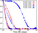
(a) HB autocorrelation

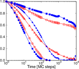
(b) Translational autocorrelation

Figure 4: Autocorrelation functions of the average hydrogen bond index $M$ (a), and of the displacement of a molecule with respect to the center of its cell (b). The functions are calculated at the state points indicated in the legend (with $T$ expressed in K and $P$ in GPa). Pressures are as in Fig. 2 and, for both pressures, the water monolayer is liquid for $T>218$ K and solid for $T\leq 218$ K: LDC at $P=0.06$ GPa and hexatic at $P=0.24$ GPa.

For each quantity we define the correlation time $\tau$ as the time at which the normalized correlation function Eq. (10) and (11) decay to $1/e$. Our calculations show that at low $P$, the hydrogen bond correlation function $C_{M}$ (Fig.4a) is exponential in the liquid phase, but has a non-exponential behavior in the LDC phase, with a correlation time $\tau$ that largely increases for decreasing $T$, as expected in the solid phase characterized by a well developed hydrogen bond network [4]. By increaing $P$, the number of hydrogen bonds largely decreases and the hydrogen bond correlation function $C_{M}$ shows a much faster decay to zero. Nevertheless, at high $P$ and low $T$ the function is not-exponential consistent with the approach of a frozen state.

For the translational autocorrelation function $C_{r}$ (Fig.4b) we find a much slower decay to zero at all the state points. For the state points corresponding to the solid phases, at low $T$ and any $P$, the function has an evident non-exponential behavior and an extremely long correlation time $\tau$, two orders of magnitude greater than $C_{M}$. This is consistent with the arrested translational dynamics of the solid phases.

Next, we analyze the behavior of the variance $\langle\delta^{2}M_{i}\rangle$ of $M_{i}$, and $\langle\delta^{2}(\delta\vec{r}_{i})\rangle$ of $\delta\vec{r}_{i}$, defined as the normalization factors of Eq.s (10) and (11), respectively (Fig.5).

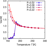
(a) HB orientation variance

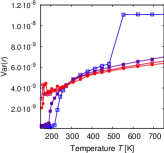
(b) Translational variance

Figure 5: The variance of the average hydrogen bond index $M_{i}$ at (a), and of the displacement $\delta\vec{r}_{i}$ of the molecule inside the cell at (b). At low $P$ both display a discontinuous decrease at the liquid-LDC first-order phase transition. At high $P$, around the liquid-hexatic second-order phase transition, $\langle\delta^{2}M_{i}\rangle$ increases continuously, while $\langle\delta^{2}(\delta\vec{r}_{i})\rangle$ has a discontinuity. At high $T$, $\langle\delta^{2}(\delta\vec{r}_{i})\rangle$ shows the discontinuity associated to the liquid-gas first-order phase transition. Pressures are expressed in GPa.

As expected, at low $P$ both variances have discontinuties at the temperature of the liquid-LDC first-order phase transition. The increase of $\langle\delta^{2}M_{i}\rangle$ for decreasing $T$ is the consequence of the increase of the fluctuations in the hydrogen bonds network at low $T$.

On the other hand, the translational variance decreases for decreasing $T$ and presents discontinuities at the first-order phase transitons, e. g. being crystal at $T<274$ K, gas at $T>483$ K and a liquid at the intermediate values at $P=0.02$ GPa. At high $P$, instead, the slowing down of the translational dynamics occurring at the liquid-hexatic coexistence is marked by a non monotonic $\langle\delta^{2}(\delta\vec{r}_{i})\rangle$, suggesting an out of of equilibrium behavior at very low $T$.

3 Conclusions

We study by efficient Monte Carlo simulations a coarse-grained model for a water monolayer in hydrophobic nanoconfinement and find two forms of ice at low $T$. At low pressure, the model reproduces the occurrence of low-density-crystal (LDC) ice with hydrogen bonds forming a square network, as observed with detailed molecular dynamics simulations. At high pressure, where detailed molecular dynamics simulations are not available, we find a hexatic ice, separated from the liquid phase by a second-order phase transition. Our structural analysis shows that the hexatic phase has solid-like long-range orientational order and liquid-like short-range translational order.

By studing the autocorrelation functions and the variances of bonding and translational parameters, we observe different behaviors at low and high $P$ that we can relate to the thermodynamic phases. The dynamics at low $T$ become slow at any pressure, and possibly fall out of equilibrium at low $T$ in the hexatic phase, before entering the high-density-crystal (HDC) ice phase.

Aknowledgement

We thank the spanish MICINN grant FIS2009-10210 (Co-financed FEDER).

References

- [1] Djamal Bouzida, Shankar Kumar, and Robert H. Swendsen. Efficient monte carlo methods for the computer simulation of biological molecules. Phys. Rev. A, 45(12):8894–8901, Jun 1992.
- [2] Kun Chen, Theodore Kaplan, and Mark Mostoller. Melting in two-dimensional lennard-jones systems: Observation of a metastable hexatic phase. Phys. Rev. Lett., 74(20):4019–4022, May 1995.
- [3] Jeffrey R. Errington, Pablo G. Debenedetti, and Salvatore Torquato. Cooperative origin of low-density domains in liquid water. Phys. Rev. Lett., 89(21):215503, Oct 2002.
- [4] G. Franzese and F. de los Santos. Dynamically slow processes in supercooled water confined between hydrophobic plates. J. Phys.: Condens. Matter, 21:504107, 2009.
- [5] G. Franzese and H. Eugene Stanley. A theory for discriminating the mechanism responsible for the water density anomaly. Physica A Statistical Mechanics and its Applications, 314:508–513, November 2002.
- [6] Giancarlo Franzese, Manuel I. Marqués, and H. Eugene Stanley. Intramolecular coupling as a mechanism for a liquid-liquid phase transition. Phys. Rev. E, 67(1):011103, Jan 2003.
- [7] V. Bianco G. Franzese and S. Iskrov. Water at interface with proteins. Food Biophysics, Dec 2010.
- [8] Pradeep Kumar, Sergey V. Buldyrev, Francis W. Starr, Nicolas Giovambattista, and H. Eugene Stanley. Thermodynamics, structure, and dynamics of water confined between hydrophobic plates. Phys. Rev. E, 72(5):051503, Nov 2005.
- [9] M. G. Mazza, K. Stokely, S. E. Pagnotta, F. Bruni, H. E. Stanley, and G. Franzese. Two dynamic crossovers in protein hydration water and their thermodynamic interpretation. ArXiv e-prints, July 2009.
- [10] I. R. McDonald. Npt-ensemble monte carlo calculations for binary liquid mixtures. Mol. Phys., 23(1):41–58, 1972.
- [11] Alexander Z. Patashinski, Rafal Orlik, Antoni C. Mitus, Bartosz A. Grzybowski, and Mark A. Ratner. Melting in 2d lennard-jones systems: What type of phase transition?†. The Journal of Physical Chemistry C, 114(48):20749–20755, 2010.
- [12] Christoph G. Salzmann, Paolo G. Radaelli, Erwin Mayer, and John L. Finney. Ice xv: A new thermodynamically stable phase of ice. Phys. Rev. Lett., 103(10):105701, Sep 2009.
- [13] A. K. Soper. Structural transformations in amorphous ice and supercooled water and their relevance to the phase diagram of water. Mol. Phys., 106:2053–2076, 2008.
- [14] Alan K. Soper and Maria Antonietta Ricci. Structures of high-density and low-density water. Phys. Rev. Lett., 84(13):2881–2884, Mar 2000.
- [15] K. Stokely, M. G. Mazza, H. E. Stanley, and G. Franzese. Effect of hydrogen bond cooperativity on the behavior of water. Proceedings of the National Academy of Science, 107:1301–1306, January 2010.
- [16] J Talbot, G Tarjus, and P Viot. Optimum monte carlo simulations: some exact results. Journal of Physics A: Mathematical and General, 36(34):9009, 2003.
- [17] Thomas M. Truskett, Salvatore Torquato, Srikanth Sastry, Pablo G. Debenedetti, and Frank H. Stillinger. Structural precursor to freezing in the hard-disk and hard-sphere systems. Phys. Rev. E, 58(3):3083–3088, Sep 1998.
- [18] R. Zangi and A. E. Mark. Bilayer ice and alternate liquid phases of confined water. Journal of Chemical Physics, 119:1694–1700, July 2003.
- [19] Ronen Zangi and Alan E. Mark. Monolayer ice. Phys. Rev. Lett., 91(2):025502, Jul 2003.