Feedback in Luminous Obscured Quasars

Abstract

We use spatially resolved long-slit spectroscopy from Magellan to investigate the extent, kinematics, and ionization structure in the narrow-line regions of 15 luminous, obscured quasars with $z<0.5$. Increasing the dynamic range in luminosity by an order of magnitude, as well as improving the depth of existing observations by a similar factor, we revisit relations between narrow-line region size and the luminosity and linewidth of the narrow emission lines. We find a slope of $0.22\pm 0.04$ for the power-law relationship between size and luminosity, suggesting that the nebulae are limited by availability of gas to ionize at these luminosities. In fact, we find that the active galactic nucleus is effectively ionizing the interstellar medium over the full extent of the host galaxy. Broad ($\sim 300-1000$ km s^-1) linewidths across the galaxies reveal that the gas is kinematically disturbed. Furthermore, the rotation curves and velocity dispersions of the ionized gas remain constant out to large distances, in striking contrast to normal and starburst galaxies. We argue that the gas in the entire host galaxy is significantly disturbed by the central active galactic nucleus. While only $\sim 10^{7}-10^{8}$ $M_{\odot}$ worth of gas are directly observed to be leaving the host galaxies at or above their escape velocities, these estimates are likely lower limits because of the biases in both mass and outflow velocity measurements and may in fact be in accord with expectations of recent feedback models. Additionally, we report the discovery of two dual obscured quasars, one of which is blowing a large-scale ($\sim 10$ kpc) bubble of ionized gas into the intergalactic medium.

1 Introduction

It has become fashionable to invoke feedback from accreting black holes (BHs) as an influential element of galaxy evolution (e.g., Tabor & Binney, 1993; Silk & Rees, 1998; Hopkins et al., 2006; Sironi & Socrates, 2010). Regulatory mechanisms are sorely needed to keep massive galaxies from forming too many stars and becoming overly massive or blue at late times (e.g., Thoul & Weinberg, 1995; Croton et al., 2006). Feedback from an accreting BH provides a tidy solution. For one thing, the gravitational binding energy of a supermassive BH is completely adequate to unbind leftover gas in the surrounding galaxy. Furthermore, using simple prescriptions for black hole feedback leads to a natural explanation for the observed scaling relations between the BH mass and properties of the surrounding galaxy, including stellar velocity dispersion and bulge luminosity and mass (e.g., Häring & Rix, 2004; Gültekin et al., 2009). The problem remains to find concrete evidence of BH self-regulation, and to determine whether or not accretion energy has a direct impact on the surrounding galaxy.

There are some special circumstances in which accretion energy clearly has had an impact on its environment. For instance, jet activity in massive elliptical galaxies and brightest cluster galaxies deposits energy into the hot gas envelope (see review in McNamara & Nulsen, 2007), although the efficiency of coupling the accretion energy to the gas remains uncertain (e.g., Bîrzan et al., 2004; Best et al., 2005; Heinz et al., 2006), as does the relative importance of heating by the active nucleus as opposed to other possible sources (e.g., Zakamska & Narayan, 2003; Sijacki et al., 2008; Conroy & Ostriker, 2008; Parrish et al., 2009). Likewise, there is clear evidence that powerful radio jets entrain warm gas and carry significant amounts of material out of their host galaxies (e.g., van Breugel et al., 1986; Tadhunter, 1991; Whittle, 1992b; Villar-Martín et al., 1999; Nesvadba et al., 2006, 2008). However, as only a minority ($\sim 10\%$) of active BHs are radio-loud, invoking this mechanism as the primary mode of BH feedback would require all galaxies to have undergone a radio-loud phase – a conjecture which lacks direct evidence and contradicts a theoretical paradigm in which radio-loudness is determined by the spin of the black hole (e.g., Tchekhovskoy et al., 2010). Thus, it is not clear whether BH activity in radio galaxies accounts for more than a small fraction of the BH growth (e.g., Sołtan, 1982; Yu & Tremaine, 2002) and therefore whether this mode of feedback is in fact the dominant one.

Nuclear activity is known to drive outflows on small scales. Broad absorption-line troughs are seen in $\sim 10-20\%$ of luminous quasars (e.g, Reichard et al., 2003), and there is good reason to believe that the outflows are ubiquitous but have a covering fraction of $\sim 20\%$, at least for high-$L_{\mathrm{bol}}/L{\mathrm{{}_{Edd}}}$ systems (e.g., Weymann et al., 1981; Gallagher et al., 2007; Shen et al., 2008). The velocities in broad absorption lines are high ($\sim 10,000$ km s^-1), and they most likely emerge from a wind blown off of the accretion disk (e.g., Proga & Kallman, 2004). In a few rare objects the outflow appears to extend out to large distances from the nucleus (Moe et al., 2009), but it is unclear whether most of these outflows have any impact beyond hundreds of Schwarzschild radii. Narrow associated absorption-line systems are signposts of outflows extending to larger distances, but determining

their physical radii (and thus the mass outflow rate) is notoriously challenging. In cases where it is possible, the estimated outflow rates are thought to be significant fractions of the accretion onto the BH (see review in Crenshaw et al., 2003).

It is clear that some quasars affect their environment some of the time. The extent and the dominant mode of these interactions remain open to interpretation. In particular, it is not clear whether quasars are effectively removing the interstellar medium (ISM) of their host galaxies during the high accretion rate episodes – those that account for the majority of the BH growth. Such feedback has been postulated by numerical simulations (e.g., Springel et al., 2005), but direct observational evidence for this process is lacking.

In this work, we look for direct evidence of extended warm gas in emission, using the narrow-line region (NLR) and specifically the strong and ubiquitous [O III]$~{}\lambda 5007$ line. The NLR is in some respects the ideal tracer of the interface between the galaxy and the active galactic nucleus (AGN), as the gas is excited by the AGN but extended on galaxy-wide scales. For a long time, following the seminal work of Stockton & MacKenty (1987), it was thought that truly extended emission-line regions (so-called EELRs with radii of 10-50 kpc) were only found in radio-loud objects. Using narrow-band imaging, these authors examined known luminous, $z\approx 0.5$ AGNs and found that $\sim 1/3$ of the radio-loud objects had luminous extended [O III] nebulosities, while none of the radio-quiet objects did. It is not clear if the extended gas has an internal or external origin nor whether it is only present in radio-loud systems or is only well-illuminated in the presence of radio jets (e.g., Stockton et al., 2006; Fu & Stockton, 2009).

Emission-line regions around radio-quiet systems (Husemann et al., 2008) are not usually as extended nor as luminous as those seen in the presence of powerful radio jets. This statement depends on the flux limit. At very low surface-brightness levels ($\sim 10^{-18}$erg s^-1 cm^-1 arcsec^-2), diverse morphologies are observed in emission line gas (e.g., Colbert et al., 1996; Veilleux et al., 2003). An interesting exception may be the broad-line active galaxy Mrk 231. This galaxy shows outflowing neutral and ionized gas that is extended on $\sim 10$ kpc scales and moving at thousands of km s^-1 (Hamilton & Keel, 1987). There is a jet in this galaxy (as well as a starburst) but the jet is not likely the source of acceleration of the neutral outflow (Rupke et al., 2005).

Rather than focus on unobscured (broad-line) quasars, where detailed study of the NLR extent and kinematics is hampered by the presence of a luminous nucleus, we look instead at obscured quasars. The experiment is worth revisiting in light of the discovery of a large sample of obscured quasars with the Sloan Digital Sky Survey (SDSS; York et al., 2000). The sample, with $z<0.8$, was selected based on the [O III] line luminosity (Zakamska et al., 2003) and now comprises nearly 1000 objects (Reyes et al., 2008). Extensive follow-up with the Hubble Space Telescope (Zakamska et al., 2006), Chandra and XMM-Newton (Ptak et al., 2006; Vignali et al., 2010), Spitzer (Zakamska et al., 2008), spectropolarimetry (Zakamska et al., 2005), Gemini (Liu et al., 2009), and the VLA (Zakamska et al., 2004; Lal & Ho, 2010) yield a broad view of the properties of the optically selected obscured quasar population. We target the low-redshift end of the sample, to maximize our spatial resolution of the NLR. In our first paper, we examined the host galaxies of our targets (Greene et al., 2009, Paper I hereafter). Here we study the spatial distribution and kinematics of the ionized gas. After describing the sample and observations (§2), we turn to the NLR sizes (§3) and then the spatially resolved kinematics of the sample as a whole (§4). We present two candidate dual obscured AGNs (§5) and then summarize and conclude (§6).

Figure 1: Three example [O III] (solid) and continuum (dotted) surface brightness profiles as a function of spatial position, plotted in units of $10^{-15}$ erg s^-1 cm^-2 arcsec^-2. In each case the line spectrum was summed over a velocity twice that of the FWHM of [O III], while the continuum was summed over a line-free band 10 times wider. The inferred [O III] (short-dashed line) diameters are shown for reference. In the center panel, we include a flux calibration star for reference (dashed).

2 The Sample, Observations, and Data Reduction

The sample and data reduction were introduced in detail in Paper I (Table 1). The sample was selected from Reyes et al. (2008). We focused on targets with $z<0.45$ to ensure that [O III]$~{}\lambda 5007$ was accessible in the observing window and imposed a luminosity cut on the [O III] line of $L_{\mathrm{[O{\tiny III}]}}\geq 10^{42}$ erg s^-1 to pre-select luminous quasars (estimated intrinsic luminosity $M_{B}<-24$ mag). Radio flux densities at 1.4 GHz were obtained from the Faint Images of the Radio Sky at Twenty cm survey (FIRST; Becker et al. 1995) and the NRAO VLA Sky Survey (NVSS; Condon et al. 1998). With one exception, all objects are radio-quiet, as determined by their position on the $L_{\mathrm{[O{\tiny III}]}}-\nu L_{\nu}$ (1.4 GHz) diagram (Xu et al., 1999; Zakamska et al., 2004), and they are at least an order of magnitude below the nominal radio-loud vs. radio-quiet separation line in this plane. The single radio-loud object in the sample, SDSS J1124+0456, is a double-lobed radio galaxy (alternate name 4C+05.50) with $\nu L_{\nu}$ (1.4 GHz)$=2.9\times 10^{42}$ erg s^-1 which was observed with a slit nearly perpendicular to the orientation of its large-scale radio lobes.

We observed 15 objects over two observing runs using the Low-Dispersion Survey Spectrograph (LDSS3; Allington-Smith et al., 1994) with a $1\arcsec\times 4\arcmin$ slit at the Magellan/Clay telescope on Las Campanas. The seeing was typically $\sim 1\arcsec$ over the two runs. We integrated for at least one hour per target and covered one or two slit positions (Table 1). Lower-$z$ targets were observed with the VPH-Blue grism in the reddest setting, for a wavelength coverage of $4300-7050$ Å, while the higher-$z$ targets were observed with the bluest setting of the VPH-Red grism ($5800-9400$ Å). The velocity resolution in each setting is $\sigma_{\rm inst}\approx 67$ km s^-1. In addition to the primary science targets, at least two flux calibrator stars were observed per night and a library of velocity template stars consisting of F–M giants was observed over the course of the run.

Since we have only long-slit observations, we do not sample the full velocity field of the gas or stars in the galaxy. With a few exceptions, the galaxy images were only marginally resolved in the SDSS images. Thus in selecting position angles to observe we were mainly guided by visual inspection of the color composite images. Since these galaxies typically have very high equivalent width [O III] lines, we attempted to identify [O III] structures based on color-gradients in the images. As a result, the slit is not necessarily oriented along the major or minor axis of a given galaxy. In particular, it is important to keep in mind when judging the radial velocity curves of the spiral galaxies (SDSS J1106+0357, SDSS J1222$-$0007, SDSS J1253$-$0341, SDSS J2126+0035 and likely SDSS J1124+0456). Of these, SDSS J1106+0357 and SDSS J2126+0035 were observed along the major axis, and SDSS J1222$-$0007 is within $20\arcdeg$ of the major axis. The others are observed at $\sim 40\arcdeg$ from the major axis. None were observed solely along the minor axis.

Cosmic-ray removal was performed using the spectroscopic version of LACosmic (van Dokkum, 2001), and bias subtraction, flat-field correction, wavelength calibration, pattern-noise removal (see Paper I), and rectification were performed using the Carnegie Observatories reduction package COSMOS. For the two-dimensional analysis discussed in this paper (e.g., the [O III] size determinations) we additionally use the sky subtraction provided by COSMOS. The flux calibration correction is determined from the extracted standard star using IDL routines following methods described in Matheson et al. (2008) and then applied in two dimensions. In the first paper we demonstrate that the absolute normalization of the flux calibration is reliable at the $\sim 40\%$ level. “Nuclear” measurements refer to the 2$\farcs$25 spatial extraction.

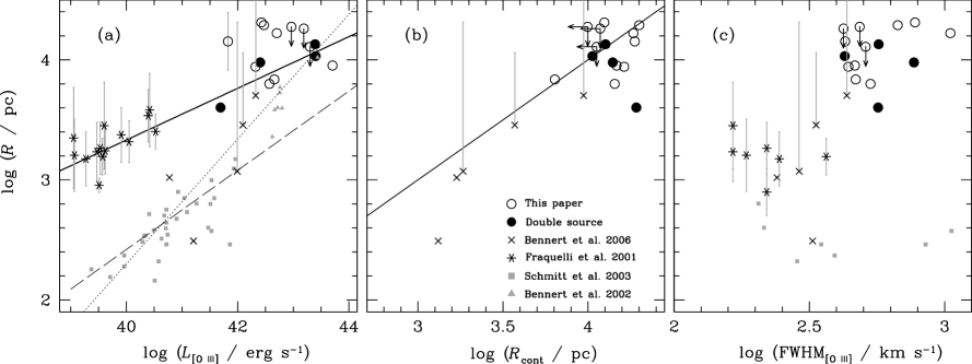
Figure 2: Radii of the [O III]-emitting regions, as measured from spatial cuts through the spectra centered on the [O III] line, compared with various other properties. Our measurements are shown in large circles and upper limits on the nebular sizes, in unresolved cases, are shown as arrows. Our estimated uncertainty of $\sim 3$ is demonstrated for one point only. We also show measurements from Bennert et al. (2002, broad-line AGNs; filled triangles), Schmitt et al. (2003, grey filled squares), Fraquelli et al. (2003, asterisks), and Bennert et al. (2006, crosses). (a): $R_{\rm[O\tiny III]}$ compared to total $L_{\mathrm{[O{\tiny III}]}}$. The two quantities are correlated (Kendall’s $\tau=0.89$ with probability $P<10^{-5}$ that no correlation is present). Our best-fit is shown with a solid line. Our emission-line regions are considerably larger at a given $L_{\mathrm{[O{\tiny III}]}}$ than either the broad-line quasars considered by Bennert et al. (2002; filled triangles and dotted line) or the relation derived by Schmitt et al. (2003; dashed line), likely due to differences in depth. Thus, we exclude the latter two in our fitting. (b): $R_{\rm[O\tiny III]}$ compared to the size of the galaxy continuum measured in a comparable fashion (see text). Here we include only the sample of Bennert et al. (2006) for comparison, since we do not have galaxy sizes available in the other cases. In general it is clear that the continuum and emission line sizes are of the same order (Kendall’s $\tau=0.52$ with $P=0.098$). The solid line shows the 1:1 relation to guide the eye. (c): $R_{\rm[O\tiny III]}$ plotted against the FWHM of the [O III] line from the nuclear extraction. Here we include FWHM measurements from Whittle (1992a) for the Bennert et al. (2006) and Schmitt et al. (2003) samples. There is clearly a trend (Kendall’s $\tau=0.75,P=3\times 10^{-4}$). The two outliers (bottom, right) are Mrk 3 and NGC 1068. However, we note that the size of NGC 1068 is likely underestimated here; Veilleux et al. (2003) find a size of $\sim 11$ kpc using a tunable filter.

3 Nebular Sizes

3.1 Measurements

The physical extent of the NLR provides one basic probe of the impact of the AGN on the surrounding galaxy. We work with the rectified two-dimensional spectra. In order to boost the signal in the spatial direction, we collapse each spectrum in the velocity direction. We use a band with a velocity width that is twice the full width at half-maximum (FWHM) of the nuclear [O III] and centered on the nuclear [O III] line (Fig. 1). The line width is measured from a continuum-subtracted spectrum, but we do not perform continuum subtraction on the two-dimensional spectra. This high signal-to-noise (S/N) spatial cut allows us to measure the NLR sizes much more sensitively than from typical narrow-band imaging. Specifically, we measure the total spatial extent of the line emission down to a $5~{}\Sigma$ limit, where $\Sigma$ is determined from spatially-offset regions of the collapsed surface brightness profile. We are reaching typical depths of $\Sigma\approx 10^{-16}$ erg s^-1 cm^-2 arcsec^-2. In three cases the nebular spectra are not spatially resolved (i.e., the spatial distribution matches that of a standard star). There are six objects for which we have multiple slit positions. The range in nebular size derived from cases with multiple slit positions is $\sim 30\%$.

In a few cases (SDSS J1356$-$1026, SDSS J2126$+0035$ & SDSS J2212$-0944$), the line ratios change as a function of radius and [O III]/H$\beta$ falls below three. This changing ratio may reflect changes in the ionization parameter or gas-phase metallicity, or a transition from ionization dominated by the AGN to H II regions (e.g., Bennert et al., 2006). By ionization parameter, we mean the ratio of the density of ionizing photons to the density of electrons. Given the luminosities of quasars in our sample and the rates of star formation in their hosts (Zakamska et al., 2008), we expect that the number of ionizing photons from the quasars exceeds that from stars by about an order of magnitude. Nevertheless, since quasar illumination is not necessarily isotropic and since photons from star formation are distributed more uniformly within the galaxy than those arising from the central engine, it is plausible that we may see gas excited by stars in the outer regions of the galaxy. Shock excitation is unlikely since the linewidths are uniformly narrow in these outer regions. To be safe, we exclude the regions with [O III]/H$\beta$$<3$ when calculating the NLR sizes. We have not applied any correction for reddening, which could be substantial (e.g., Meléndez et al., 2008). Reyes et al. (2008) show that deriving robust extinction corrections for the SDSS obscured quasars is not straightforward, and we neglect such corrections here.

One of the objects in our sample, SDSS J1356+1026, has a much more dramatic extended emission-line nebula than the rest (Figure 3.2). We will discuss the detailed kinematics and energetics of this object in more detail in a parallel paper (Greene & Zakamska in preparation). For the present work, we explore the implications of detecting one single extended emission-line region in the sample (§6).

We should note that deriving nebular sizes is an ill-defined task. First of all, ionized nebulae need not have regular shapes, and so the definition of size is not necessarily well-defined. This difficulty is only exacerbated when long-slit spectra are used to define the size, since our slit may well miss spatially extended regions. Furthermore, the concept of size depends sensitively on the depth of the observation. Deep observations probing depths of a few times $10^{-18}$ erg s^-1 cm^-2 arcsec^-2 indeed reveal faint, extended gas with a range of morphologies (e.g., Veilleux et al., 2003). Thus, the primary size uncertainties are in these systematics, which dwarf the measurement errors.

We quantify the uncertainties in the following manner. First of all, since we have not included surface brightness dimming, there is a dispersion of $\sim 0.1$ dex in the sizes due to distance. Secondly, and more important, narrow-line regions are not strictly round. Thus, depending on the position of the long-slit, we may derive a different answer. We have found, for the six objects with multiple slit positions, that the sizes agree within $30\%$. Finally, and most difficult to quantify, the shape will likely grow more irregular as we push to lower flux limits. We have attempted to quantify this dispersion in emission line profile using the ratio between the luminosity-weighted mean width of each spatial [O III] profile and the adopted radius measured down to a fixed surface brightness. Were the NLRs all of the same shape, then the mean width would be a fixed fraction of the total size. Instead, the ratio ranges from 0.2 to 4, with a typical value of three. We thus adopt a factor of three as the overall uncertainty in the sizes. Additionally, we flag as particularly uncertain those systems with a nearby massive companion galaxy, since there we are further contaminated by tidal gas.

3.2 Obscuration, Ionization, and Excitation

NLR sizes have been measured from narrow-band imaging (Mulchaey et al., 1996a; Bennert et al., 2002; Schmitt et al., 2003) and from long-slit spectroscopy (e.g., Unger et al., 1987; Fraquelli et al., 2003; Bennert et al., 2006). Narrow-band imaging is preferable for studying the NLR morphology, but reaches shallower limits than the spectroscopy.

Left: Image ($r-$band) of the merging galaxies SDSS J1356+1026. Scale bar indicates 10″ (22 kpc). N is down and E to the right. Right: The two-dimensional spectrum centered on the continuum-subtracted [O III]$~{}\lambda 5007$ line. Oriented as the image. The spectrum spans 1814 km s^-1in the velocity (x) direction.

Integral-field observations allow one to study two-dimensional kinematics (Humphrey et al., 2010), but for local objects only cover the inner NLR (e.g., Barbosa et al., 2009).

We compile a comparison sample of lower-luminosity obscured AGNs with measured NLR sizes from the literature (Bennert et al., 2002; Schmitt et al., 2003; Bennert et al., 2006; Fraquelli et al., 2003). We include the Bennert et al. (2002) and Schmitt et al. (2003) measurements in Fig. 2 for completeness, but note that the sizes cannot be compared directly with those we measure here, because of the difference in depth. The limiting surface brightness values that we achieve in this work are at least a factor of 10 deeper than these narrow-band imaging studies from space, which range from $\sim 10^{-15}-3\times 10^{-14}$ erg s^-1 cm^-2 arcsec^-2. For this reason, we do not include the space-based measurements in any analysis presented here (e.g., fitting of relationships). Fraquelli et al. do not quote sizes but rather provide power-law fits to the surface brightness as a function of distance to the nucleus. Taking their functional form, we calculate sizes that match our limiting surface brightness of $\sim 10^{-16}$ erg s^-1 cm^-2 arcsec^-2. For uniformity, we calculate sizes for Bennert et al. (2006) in the same way, and we adopt their smaller radii in cases where star formation dominates in the outer parts. In cases of overlap between works, we prefer the Bennert et al. (2006) observations, since they are both sensitive and take into account photoionization by starlight. The measurements for our sample are summarized in Figure 2 and Table 2, while the comparison samples are shown in Figure 2.

The observed distribution of NLR gas depends on the geometry and luminosity of the ionizing source, the geometry and kinematics of the host ISM (e.g., disk, spherical, outflow, or infall), and the density distribution of the gas. While most of these are likely related to the morphology and dynamical state of the galaxy, the geometry of the ionizing source is tied to the orientation of the AGN. In the simplest model, the galaxy ISM is spherically distributed, while the ionizing radiation from the AGN emerges anisotropically along lines of sight unaffected by the circumnuclear ‘torus’, as postulated by unified models of AGN activity. In this case we expect to see ionization cones when the beam is not pointed directly at us, reflecting the geometry of circumnuclear obscuration. Such cones are observed in images of nearby Seyfert galaxies (Pogge, 1988; Tadhunter & Tsvetanov, 1989; Storchi-Bergmann et al., 1992) and more recently in the luminous obscured quasars studied here (Zakamska et al., 2006).

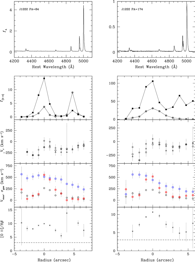
Figure 3: Resolved spectroscopic measurements for SDSS J1222$-0007$. In the top panel we show the central spectrum, extracted within the inner $\sim 1\arcsec$, arbitrarily normalized. Then we show the flux in the [O III] line (filled black squares) and the continuum (open stars) as a function of radius (10^-15 erg cm^-2 s^-1). In the third panel we show the radial velocity curve of the peak of [O III] (open triangles), the velocity of the peak of the H$\beta$ line (open circles), and the luminosity-weighted mean velocity of [O III] (open squares). In the fourth panel the velocity dispersion of the [O III] line (open black circles) is compared with the maximum velocity (the velocity at $20\%$ of the line maximum) to the red (red open circle with cross) and the blue (blue open circle with dot). In the final panel the ratio of [O III]/H$\beta$ is plotted (black crosses). A ratio of [O III]/H$\beta$ of three is noted with the dashed line.

In this simplest geometry, we would expect to find smaller sizes in unobscured sources, when looking closer to the axis of the ionization cones. The difference in distributions depends on the expected opening angle of the torus, with larger difference for smaller opening angles. Recent observations of obscured quasars suggest that the space densities of obscured and unobscured sources are $\sim$ equal (Reyes et al., 2008), leading to opening angles of $\lesssim 120\arcdeg$, but even if significantly smaller opening angles are assumed, the expected differences in the median projected size between the two populations is small ($\lesssim 0.2$ dex). At low redshift and (thus) lower luminosity, ionization cones are also observed in unobscured sources (e.g., Evans et al., 1993; Boksenberg et al., 1995), while round NLRs are observed in both types (Mulchaey et al., 1996b). Presumably, the ISM is not always spherically distributed or relaxed (Mulchaey et al., 1996b; Schmidt et al., 2007).

In Figure 2a it appears that the NLR sizes of our obscured quasars are larger than the unobscured ones (median difference 0.4 dex). However, this difference can be explained by differences in the depths of the observations, thus we cannot address orientation differences in detail from these samples. It is interesting to note that at lower luminosities, Schmitt et al. (2003) do not see a significant size difference between the two populations. These observations, while shallow, are uniform between the obscured and unobscured populations.

There has been some debate in the literature about the slope of a purported correlation between the NLR size and the AGN luminosity (e.g., Bennert et al., 2002; Schmitt et al., 2003; Bennert et al., 2006). Some correlation is expected, given that the AGN is photoionizing the NLR gas, but the form it takes may tell us something about covering factor or density as a function of luminosity. It is clear from Figure 2(a) that generally larger NLRs are found in more luminous objects (Kendall’s $\tau=0.89$ with probability $P<10^{-5}$ that no correlation is present). It is also clear that there is substantial scatter; we find an rms scatter of 0.3 dex in radius at fixed $L_{\mathrm{[O{\tiny III}]}}$. We performed Monte Carlo simulations of ionization cones observed at random directions (restricted to be outside the cones). They suggest that the orientation of the NLR axis relative to the line of sight is not a significant source of the observed scatter. At a fixed NLR size, orientation effects introduce a scatter of $<0.15$ dex within each (obscured or unobscured) subpopulation, even when a wide range of opening angles is allowed for. Therefore, the observed scatter is likely due to the combination of the true variance in NLR sizes at a given luminosity and to the differences in the definition of NLR “size”. For instance, Bennert et al. (2006) derive sizes that are factors of $\sim 2$ larger than those based on HST narrow-band imaging because of their increased sensitivity. Given that the NLR is not always spherically symmetric or smooth, defining a meaningful size that is insensitive to depth is a difficult problem.

For completeness, we fit a power-law relation between $L_{\mathrm{[O{\tiny III}]}}$ and NLR size, using all narrow-line comparison samples as well as the objects considered here. Because there are upper limits on the sizes, we calculate a linear regression using the binned Schmitt method, from the Astronomy Survival Analysis (ASURV) software as implemented in iraf (Feigelson & Nelson, 1985; Isobe et al., 1986). The fit is shown in Figure 2. We find:

$${\rm log}(R_{\rm NLR}/10^{3}{\rm pc})=(0.22\pm 0.04)\,{\rm log}(L_{\rm[O{\tiny III}]}/10^{42}{\rm erg~{}s^{-1}})$$ (1)

$$+(3.76\pm 0.07).$$

The shallow slope we observe is consistent with a picture in which the nebulae are matter-bounded. At the distances from the quasar that we are probing with our observations, the density of material is low enough that the emissivity is no longer limited by the flux of photons by the quasar, but rather by the low density of the gas, and a large fraction of photons can escape into the intergalactic medium. Note that the correlation between AGN continuum luminosity and $L_{\mathrm{[O{\tiny III}]}}$ in broad-line AGNs (e.g., Yee, 1980) suggests that the nebulae are limited by the number of photons in the bright central regions of the galaxy, but that the situation changes in the diffuse outer parts. If so, we would expect size to scale as the square-root of luminosity at low luminosities and then flatten out to at high luminosities, modulo differences in host galaxies.

In addition to measuring the nebular sizes, we also parameterize the luminosity drop in the outer parts as a power-law and measure the power law slope ($L_{\mathrm{[O{\tiny III}]}}$$\propto r^{-\beta}$). The slopes range from $1.6<\beta<3.8$ (Table 2). These slopes correspond to density profiles with slopes ranging from 1.3 to 2.4, in good agreement with the HST observations of Zakamska et al. (2006).

One concern, as pointed out by Netzer et al. (2004), is that eventually the ionizing photons will run out of interstellar medium to ionize, particularly in the most luminous quasars. The NLR size cannot in general grow indefinitely beyond the confines of the host galaxies. In Figure 2(b), we compare the continuum and nebular sizes. Rather than using effective radii of host galaxies from photometry, we use the same method to measure the continuum extent as we used for the [O III] lines, collapsing the two-dimensional spectrum in the spectral direction over line-free regions to boost the signal. Galaxy sizes are weakly correlated with NLR size (Kendall’s $\tau=0.52$ with $P=0.0975$). We see that the NLR sizes are comparable to the galaxy continua. The exception is SDSS J1356+1026, which contains the spectacular bubble shown below. At these luminosities, the AGN is effectively capable of photoionizing the entire galaxy ISM, as well as companion galaxies out to several tens of kpc, as we saw in some of our previous long-slit observations (Liu et al., 2009).

Outflowing components of the NLR are routinely seen in radio galaxies (e.g., McCarthy, 1993; Villar-Martín et al., 1999), as well as in Seyfert galaxies (e.g., Crenshaw & Kraemer, 2000; Rupke et al., 2005). On small scales, detailed modeling of the inner ($<300$ pc) NLRs of a few local AGNs with HST indicates a surprising uniformity in behavior, with $v\propto r$ along an evacuated bicone (Crenshaw & Kraemer, 2000; Crenshaw et al., 2000; Ruiz et al., 2001). Interestingly, we see similar qualitative behavior in SDSS J1356+1026 (Greene & Zakamska in prep). However, in general, NLR kinematics on larger scales are not as uniform, with mechanisms ranging from jet acceleration to radiation pressure driving (e.g., Ruiz et al., 2001; Groves et al., 2004; Rupke et al., 2005). For a complete review, see Veilleux et al. (2005). We do find some correlation between FWHM and luminosity (Figure 2c; Kendall’s $\tau=0.75,P=3\times 10^{-4}$). We will argue below based on the observed large velocity dispersions at large radius that the AGN energy is stirring up the gas on large scales, thus explaining this correlation.

4 Two-Dimensional Analysis

Maximum velocity as a function of radius. The maximum velocity is measured as the velocity at 20% of the line peak, as referenced to the systemic velocity of the stars. At each position we show the maximum red- (red circle) and blue-shifted (blue circle) velocity. While there is extended emission in nearly all targets, the typical velocities are not higher than $\sim 400$ km s^-1 for the majority of the targets. SDSS J1356+1026 is highlighted with large black circles. The dashed line highlights a velocity of $500$ km s^-1, which is the approximate escape velocity for these galaxies at $r_{e}$. We note that the effective radii of these galaxies, for which we have well-resolved imaging, range from $1\pm 0.4$ to $11\pm 2$ kpc, with a median of $3\pm 0.6$ kpc.

In this section we present the results of our two-dimensional analysis on the long-slit spectra. First we present velocity and dispersion profiles, as well as emission line ratios, as a function of position. To obtain these measurements, we extract spectra at uniform intervals as a function of spatial position along the slit. We start with rectified two-dimensional spectra from COSMOS. Each spectrum is extracted with a width of 0$\farcs$95 (5 pixels) to match the typical seeing of the observations. The central spatial position is determined by the spatial peak in the [O III] emission. The systemic velocity is determined from the absorption lines. Galaxy continuum subtraction is performed for each spectrum using a scaled version of our best-fit model from the nuclear spectrum, with only the overall amplitude allowed to vary. While this is not strictly speaking a correct model, we have insufficient S/N in the off-nuclear spectra to constrain velocity or velocity dispersion, let alone changes in stellar populations.

Once the continuum-subtracted spectra are in hand, we fit the H$\beta$+[O III]$~{}\lambda\lambda 4959,5007$ lines for each spectrum as in Paper I (see also Ho et al., 1997; Greene & Ho, 2005). Each line is modeled as a sum of Gaussians (a maximum of two for H$\beta$ and three for [O III]). The relative wavelengths of each transition and the ratio of the [O III] lines are fixed to their laboratory values, but the central velocity and line widths are allowed to vary from spectrum to spectrum. From these fits we are able to derive velocity, velocity dispersion, and line-ratio profiles as a function of spatial position. We report three measures of velocity at a given position, the peak in the [O III] line, the peak in the H$\beta$ line, and the flux-weighted mean velocity in the [O III] line. The velocity dispersion is measured as the FWHM of the [O III] model divided by 2.35. At each spatial position we also measure the “maximum” and “minimum” velocities as the velocities at $20\%$ of the [O III] peak intensity (e.g., Rupke et al., 2002) relative to the systemic velocity of the stars (shown as blue bullseyes and red crosses, respectively, in Figure 3.)

Errors are derived from Monte Carlo simulations. For each spectrum we generate 100 mock spectra using the best-fit parameters at that radius and the S/N of the original spectra. We fit each mock spectrum and the quoted parameter errors encompass $68\%$ of the mock fit values.

4.1 Radial Velocity Curves

In Figure 3 we present a representative radial velocity curve for SDSS J1222$-0007$. The remainder are shown in the Appendix. First, we note that overall the radial velocity curves are flat. In Paper I we presented detailed two-dimensional photometric fitting of these galaxies (with the exception of SDSS J1124+0456 and SDSS J1142+1027). Using these fits, we divide the sample by the bulge-to-total ratio (B/T), and call galaxies with B/T$\leq 0.1$ disks (SDSS J1106+0357, SDSS J1222$-$0007, SDSS J1253$-$0341, and probably SDSS J1124+0456), while the rest are bulge dominated. Additionally, those with clear tidal signatures are “disturbed” (SDSS J0841+0101, SDSS J1222$-$0007, SDSS J1356+1026, and SDSS J2212$-$0944). We would expect to see the signature of rotation most clearly in disk-dominated galaxies. We note once again that SDSS J1106+0357 and SDSS J2126+0035 were observed along the major axis, SDSS J1222$-$0007 was within $20\arcdeg$ of the major axis, and the remaining two galaxies were observed at a $\sim 40\arcdeg$ angle to the major axis. We would expect to see the signature of rotation in most of these galaxies. Instead, we only see rotation in the case of SDSS J1106+0357, SDSS J1124+0456, SDSS J1142+1027, and SDSS J2212$-$0007. Although with such a wide range of position angles, and such a small sample, it is hard to say for sure, we find it suggestive that neither SDSS J1253$-$0341 nor SDSS J2126+0035 shows rotation.

The sample galaxies showing rotation in their radial velocities also tend to show declines in $\sigma_{\rm g}$ by factors of two or more in the outer parts (e.g., SDSS J1124+0456). In contrast, those galaxies with flat radial velocity curves (the majority in this sample) also have notably flat $\sigma_{\rm g}$ distributions at kpc scales. Again, this is strongly in contrast to the kinematics in the stars, even in bulge-dominated systems (e.g., Jorgensen et al., 1995). More to the point, it is in contrast to the kinematics of warm gas in inactive late-type (e.g., Pizzella et al., 2004) and early-type (e.g., Fillmore et al., 1986; Bertola et al., 1995; Vega Beltrán et al., 2001) spiral galaxies.

In Paper I we showed that $\sigma_{\rm g}$ in the nucleus is uncorrelated with $\sigma_{\ast}$. Again, this behavior is in striking contrast not only to inactive galaxies but also to local, lower-luminosity active galaxies, for which it has been long been known that on average $\sigma_{\rm g}$/$\sigma_{\ast}$$\approx 1$ (e.g., Nelson & Whittle, 1996; Greene & Ho, 2005; Ho, 2009). Here we are making a stronger statement. Not only is the luminosity-weighted gas dispersion uncorrelated with the dispersion in the stars, but the dispersion in the gas stays high out to kpc scales in these galaxies. These observations provide new reason to doubt that gas velocity dispersions can be substituted for stellar velocity dispersions in luminous AGNs (e.g., Shields et al., 2003; Salviander et al., 2007).

Nuclear [O III] luminosity compared with the maximum gas velocity for each object. The maximum velocity plotted here is the largest that we measure for any individual object, although we exclude the maximum velocity in the nuclear spectrum. No correlation is apparent between the two (Kendall’s $\tau=0.13$ with a probability, $P=0.73$ of no correlation).

This behavior is different from that seen in regular inactive galaxies. It is also different from that in local, well-observed Seyfert galaxies. Previous work looking at the kinematics of lower-luminosity local Seyfert galaxies has found evidence for a two-tiered NLR structure (e.g., Unger et al., 1987). In such objects, the inner or classical NLR extends to a few hundred pc and has linewidths of $\mathrel{\hbox{\hbox to0.0pt{\hbox{\lower 4.0pt\hbox{$\sim$}}\hss}\hbox{\raise 2.0pt\hbox{$>$}}}}500$ km s^-1. At higher spatial resolution, there is clear evidence for outflow in the inner hundreds of pc in well-studied objects (e.g., Crenshaw et al., 2000; Crenshaw & Kraemer, 2000; Ruiz et al., 2001; Barbosa et al., 2009). In contrast, at larger radius, the linewidths drop and the kinematics of the NLR gas simply reflect that of the bulge or disk in which the gas sits (e.g., Nelson & Whittle, 1996; Greene & Ho, 2005; Walsh et al., 2008). Clearly, the observed kinematics of gas in hosts of obscured quasars are quite dissimilar from this picture.

Many of the host galaxies of our obscured quasars have nearby companions and/or show signs of recent interactions. It is therefore possible that the gas is being stirred by gravitational interactions with nearby galaxies. To explore that possibility further, we examine the analogous inactive ultra-luminous infrared galaxies. The integral-field spectra of Colina et al. (2005) show that even in these ongoing mergers the gas kinematics traces that of the stars. The $\sigma_{\rm g}$ profile is typically seen to decline in the outer parts as in non-merging systems, again in contrast to our findings for hosts of obscured quasars. Of course, there are exceptions in the Colina et al. sample, where the gas velocity dispersions are very complex. On the other hand, the mergers are more advanced in general than in our sample. Thus, while we cannot rule out gravitational effects in all cases, it seems most likely that the nuclear activity is directly responsible for stirring up the gas. We now address whether there is evidence for bulk motions (e.g., large-scale outflows) in the gas based on the kinematics.

Fraction of the [OIII] emission line luminosity emerging at a velocity greater than the escape velocity for all objects where the escaping fraction exceeds 10% in at least one shell. Object names are labeled with the first four digits of the full position. The escape velocity is approximated from the measured velocity dispersion assuming that $v_{c}=\sqrt{2}\sigma_{\ast}$ and that the halo has a radius of 100 kpc. We then simply integrate the part of the line with velocities greater than the escape velocity. Here we show the fraction of the line emission that is in this high-velocity component as a function of radius from the slit center.

4.2 Maximum Velocities

We have derived “maximum” red- and blueshifted velocities at $20\%$ of the line profile, relative to the systemic velocity of the stars. We examine the distribution of maximum velocities as a function of radius for the ensemble of spectra in Figure 4. While the emission extends to kpc scales for the majority of the targets, the gas velocities are not typically very high. The median maximum blue velocity at 8 kpc is $\langle v_{\rm blue}\rangle=400\pm 70$ km s^-1 while towards the red it is $\langle v_{\rm red}\rangle=330\pm 50$ km s^-1, where we quote errors in the mean. A few objects (SDSS J1253$-0341$, SDSS J1222$-0007$) have gas at velocities exceeding 500 km s^-1. We note that the effective radii of these galaxies, for which we have well-resolved imaging, range from $1\pm 0.4$ to $11\pm 2$ kpc, with a median of $3\pm 0.6$ kpc. These velocities exceed the velocity dispersions of the galaxies, but they do not compare to the $\sim$ thousands of km s^-1 outflow velocities seen by Tremonti et al. (2007) and postulated to be driven by recent AGN activity. Furthermore, they are not close to the escape velocity needed to actually unbind the gas. As we show in Figure 4.1, there is no evidence for a correlation between the nuclear $L_{\mathrm{[O{\tiny III}]}}$ luminosity and the maximum observed velocity (Kendall’s $\tau=-0.10$ with a probability $P=0.8$ of no correlation).

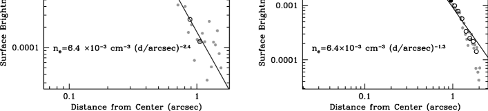
Figure 4: The measurements of the scattered light emission made in the rest-frame UV band using the HST can be translated into a constraint on the density of scattering particles. Grey points are all measurements from the HST images of Zakamska et al. (2006), while fitting was done with the large symbols, and open symbols are binned. The observed surface brightness of scattered light (vertical axis) as a function of distance $r$ from the center of the galaxy (horizontal axis) is proportional to the illuminating flux from the central AGN, $L/(4\pi r^{2})$, to the scattering cross-section of particles, ${\rm d}\sigma/{\rm d}\Omega$, and to the column density of scatterers $\simeq n_{s}r\beta$, where $\beta$ is the opening angle of the scattering region. Solid lines show the best power-law fit to electron density necessary to reproduce the scattered emission, assuming that scattering is due to dust particles. Per given hydrogen density, dust particles are about 60 times more efficient scatterers than electrons, even if the gas is fully ionized. The measurements are made using host-galaxy-subtracted images at about rest-frame 3100Å. The deficit of light in the central parts is due to the PSF smearing and dust obscuration.

We now quantitatively address whether any of the gas is approaching the escape velocity. Following Rupke et al. (2002), we calculate an approximate escape velocity for each galaxy by assuming that the circular velocity scales with the velocity dispersion as $v_{c}=\sqrt{2}\sigma_{\ast}$. Assuming the potential of an isothermal sphere, the escape velocity as a function of radius scales as:

$$v_{\rm esc}(r)=\sqrt{2}v_{c}[1+{\rm ln}(1+r_{\rm max}/r)]^{0.5}.$$ (2)

Although $r_{\rm max}$ is unknown, the escape velocity depends only weakly on its value. Thus we assume $r_{\rm max}=100$ kpc in all cases. The escape velocities thus estimated range from 500 to 1000 km s^-1 over the entire sample, but only vary by $\sim 60\%$ for an individual object over the range of radii that we probe.

With escape velocities in hand, we can now address what fraction of the line emission comes from gas that is moving at or above the escape velocity. We first ask whether there is gas exceeding the escape velocity at each radius. With the same definition of systemic velocity as above, we integrate the line emission that exceeds the escape velocity to either the red or blue side of the systemic velocity. We then normalize by the total flux at that radius. These fractions are plotted as a function of radius in Figure 4.1 for the 5 objects in which at least $10\%$ of the gas is nominally escaping for at least one radial position. For illustrative purposes, we focus here on the blue-shifted gas. In addition to calculating the escaping fraction at a given radius, we can also calculate an overall escaping fraction. They range from $<1\%-25\%$ with a median value of 2%.

Nominally only a small fraction of the NLR gas is moving out of the galaxy at or around the escape velocity. However, the projection effects may be severe, and especially so because in obscured objects the gas motions are expected to occur largely in the plane of the sky. Therefore, our estimates are a lower limit on the actual escape fractions (see §6 for details). Furthermore, as discussed further below, we have good reason to think that the medium is clumpy. Depending on whether the outflowing component has the same clumping factor as the bound gas, it is difficult to translate these observed fractions into mass fractions.

In addition to the escaping fraction, we would like to know how much mass is involved in the outflow. The standard method of estimating the density of the emission line gas uses density diagnostics such as the ratio of [S II]$~{}\lambda 6716/\lambda 6731$ or [O II]$\lambda 3729/\lambda 3726$. Neither of these is available in the Magellan spectra, and with several hundred km s^-1 velocities, the [O II] doublet is blended enough to be difficult to measure. The continuum-subtracted SDSS spectra that integrate all emission within the 3″ fiber yield a measurement of the [S II]$~{}\lambda 6716/\lambda 6731$ ratio for all but the highest redshifts. Using the iraf task temden, these can be translated into densities ranging from 250-500 cm^-3, with a mean of 335 cm^-3. These values are consistent with those commonly seen in spatially resolved observations of extended NLRs and used in mass estimations (e.g., Nesvadba et al. 2006; Fu & Stockton 2009 and many others). However, such measurements can be highly biased toward high densities in clumpy gas. Specifically, the recombination line luminosity depends on density as $L\propto\int{\rm d}V\alpha n_{e}n_{p}$, whereas mass goes like $M\propto\int{\rm d}Vn_{p}$, so the mass of the gas, its density and degree of clumpiness and its line luminosity are related through

$$M_{g}=1.7\times 10^{9}L_{H\beta}^{41}\langle n_{e}\rangle^{-1}\kappa^{-1}M_{\sun}.$$ (3)

Here we used a recombination coefficient $\alpha=1.62\times 10^{-14}$ cm³ s^-1 appropriate for a 20,000 K gas, and $\kappa=\langle n_{e}^{2}\rangle/\langle n_{e}\rangle^{2}$ is the degree of clumpiness, which by definition is $\geq 1$ and can be substantially greater. We have adopted a higher temperature than typical based on the [O III]$~{}\lambda 4363\AA$/[O III]$~{}\lambda 5007\AA$ line ratio. In general, the ratio ranges from $\sim 0.01$ in the central regions to $\sim 0.04$ further out. These ratios correspond to $T=11000-23000$K, and thus we adopt a temperature representative of the outer regions.

The standard method of calculating the mass involved amounts to using this equation with $\kappa=1$ and $n_{e}$ of a few $\times 100$ cm^-3, and produces an absolute minimum on the gas mass visible in the emission lines of a few $\times 10^{7}M_{\sun}$. However, such high densities are in direct conflict with our observations. For one thing, we see high [O III]/H$\beta$ ratios, and thus high ionization parameters, and presumably low densities, at large radius. Also, the observed extended scattering regions in obscured quasars place an independent constraint on gas densities (Zakamska et al., 2006). Scattered light flux is $\propto\int{\rm d}Vn_{s}$, where $n_{s}$ is the density of scattering particles, electrons or dust. Assuming purely electron scattering, HST observations can be fit by density profiles that decline as $r^{-(1.5-2.5)}$ and with density $\langle n_{e}\rangle=1$ cm^-3 at a distance of about 3 kpc from the center (Figure 4). The scattering angle is not well known, but it introduces only about a factor of two uncertainty in this measurement. Dust particles are even more efficient scatterers than electrons, so in the more realistic case of dust scattering, which is suggested by several lines of observational evidence (Zakamska et al., 2005), the implied mean density is constrained to be even smaller, $\langle n_{e}\rangle(1{\rm kpc})\sim 0.016$ cm^-3. The uncertainties are larger in the case of dust scattering, because the density measurement is sensitive to the assumed gas-to-dust ratio and the scattering angle (for this particular value, 90° and Small Magellanic Cloud dust, Draine 2003), but nevertheless it is clear that the scattered light observations require much lower densities than those implied by [S II] ratios. The two measurements can be reconciled if the gas is highly clumped, so that most of the luminosity is coming from high-density clumps, whereas the mass and the scattering cross-section are dominated by low-density gas.

While a detailed modeling of all observables is beyond the scope of this paper, we use a toy model in which the mass of the emitting gas at each density is a power-law function of the density, with power-law index $-\alpha$ between $n_{\rm min}$ and $n_{\rm max}$, to estimate the clumping factor. Since the [S II] line ratios are usually observed to be between the low-density and the high-density asymptotes, values of $n_{\rm max}=$ a few times the critical density are required; we use $n_{\rm max}=10^{3}$ cm^-3. At the same time, for $1<\alpha<2$ the minimal density is constrained to be $n_{\rm min}=(1-\alpha)\langle n_{e}\rangle/\alpha$ by the scattering observations. With these constraints, the clumping factor is

$$\kappa=\frac{(1-\alpha)^{2}}{\alpha(2-\alpha)}\left(\frac{n_{\rm max}}{n_{\rm min}}\right)^{2-\alpha}.$$ (4)

For example, for $\alpha=1.5$ and $\langle n_{e}\rangle=0.016$ cm^-3, for each $10^{41}$ erg s^-1 of H$\beta$ emission, the mass of the emitting gas is $M_{g}=7\times 10^{8}M_{\sun}$. This estimate can only be considered very approximate, since the derived mass is quite sensitive to the specific assumptions about clumping (for example, it varies by 2 dex as $\alpha$ varies between 1 and 2). Nevertheless, we point out that the standard method of mass determination likely produces an underestimate of the true mass and that the scattering observations provide a valuable constraint on the physical conditions in the NLR.

In short, we see compelling evidence that the NLR is clumpy. As a result, it is difficult to estimate robust gas masses, and thus difficult to determine what fraction of the gas may be expelled by potential AGN outflows.

5 Two Candidate Dual Obscured Quasars

Many recent surveys have identified potential dual active galaxies (i.e., two active galaxies with $\sim$ kpc separations) as narrow-line objects with multiple velocity peaks in the [O III] line in SDSS spectra (e.g., Wang et al., 2009; Liu et al., 2010b; Smith et al., 2010), as well as from the DEEP2 redshift survey (Gerke et al., 2007; Comerford et al., 2009b). Other candidates have been identified based on spatially offset nuclei (Barth et al., 2008; Comerford et al., 2009a). There are two intriguing objects in this sample that may contain dual AGNs.

$r$-band image of the dual AGN SDSS J0841+0101. The primary object (A) is indicated with the black arrow, red arrow points North, and the scale bar is 10″ long. Separation between the two AGNs is 3.8 ″ (7.6 kpc).

The first is SDSS J1356+1026 (Fig. 3.2), which has two clear continuum sources, each with associated high-ionization [O III] emission. Their separation is $\sim 2.5$ kpc (1$\farcs$1). This object was highlighted as a potential dual AGN by both Liu et al. (2010b) based on multiple velocity peaks in the SDSS spectrum and by Fu et al. (2010) from Keck AO imaging. We have recently shown that $\sim 10\%$ of the double-peaked narrow-line candidates also have spatially resolved dual continuum sources (Liu et al., 2010a). It seems natural that two galaxies would contain two BHs. On the other hand, there well may be a single radiating BH that is illuminating all of the surrounding gas. Unfortunately, our long-slit spectra do not include [O II] or [S II], which would give us a handle on the electron densities, and thereby whether a single ionizing source is plausible. Given the projected separation of 2.5 kpc, if we assume that there is a single ionizing source associated with one of the two continua, we would expect to see the ionization parameter decrease by a factor of $\sim 6$ between the two targets. In fact, the [O III]/H$\beta$ ratios are within $10\%$ of each other, as are the [O III] fluxes. On the other hand, the very high ionization parameter seems to extend over the entire nebulosity ($\sim 10$ kpc). Of course, the accreting BH may sit between the two continuum sources. Definitive proof requires the detection of X-ray or radio cores associated with each continuum source.

SDSS J0841+0101 shows much less ambiguous evidence for a pair of accreting BHs, with a projected separation of 3$\farcs$8 (7.6 kpc; Fig. 5). It would not be included in double-peaked samples assembled from the SDSS because the separation on the sky between the two components is larger than the SDSS 3″ fibers. Nevertheless, the component separations are comparable to those in the Liu et al. sample. Liu et al. (2010a) show that the double-peaked samples are probably dominated by single AGNs. These observations highlight that we are likewise missing dual AGNs with slightly larger separations.

As is apparent from Figure 5, the two AGNs are strikingly similar in spectroscopic properties. The [O III] luminosities ($\approx 10^{42}$ erg s^-1) agree within $<0.1$ dex, and the [O III]/H$\beta$ ratios ($\sim 10$) agree within $5\%$. The only clear difference is in the linewidths. The primary galaxy (A) has a $\mathrm{FWHM}_{\mathrm{[O\tiny III]}}$$=430$ km s^-1, while the companion AGN (B) is narrower, with $\mathrm{FWHM}_{\mathrm{[O\tiny III]}}$$=330$ km s^-1. This difference most likely reflects the fact that A, with a stellar velocity dispersion of $\sigma_{\ast}=214\pm 29$ km s^-1 is more massive than B, with $\sigma_{\ast}=150\pm 40$ km s^-1. Taken at face value, this difference in dispersions corresponds to a difference of a factor of nearly 10 in BH mass between the two galaxies. Accordingly, if the [O III] luminosity tracks the bolometric luminosity, then apparently B is accreting 10 times closer to its Eddington limit than A.

Alternatively, there may be only a single radiating black hole. If there is only one quasar – in galaxy A – then we consider two scenarios. The first is that the quasar in A is unobscured as seen from B, so that the galaxy B is photoionized by the central engine in A. If we assume that most of the NLR emission in A is produced at a distance $\lesssim 1$ kpc from the nucleus, then in order to preserve the ionization parameter (as evidenced by the similar spectra of A and B), the difference in electron density between the two galaxies would have to be a factor of $\gtrsim 60$. While the dust particles in galaxy B may scatter quasar spectrum, this emission cannot dominate the observed spectrum (otherwise we would see a broad-line AGN in source B). The resulting estimates of the emerging equivalent width of the emission lines suggest that this scenario is possible, but has to be quite tuned in order to fit observations. The second scenario is that galaxy B is located along the obscured direction, just like the observer, but scatters some of the A’s [O III] emission. However, in this scenario the ratio of [OIII] fluxes of B and A corresponds to the fraction of photons that B intercepts, $\sim(2/7.6)2/4\pi=0.006$, contrary to the observed similarity of fluxes. In conclusion, the picture of a single active black hole producing two objects with similar fluxes and ionization parameters appears unlikely.

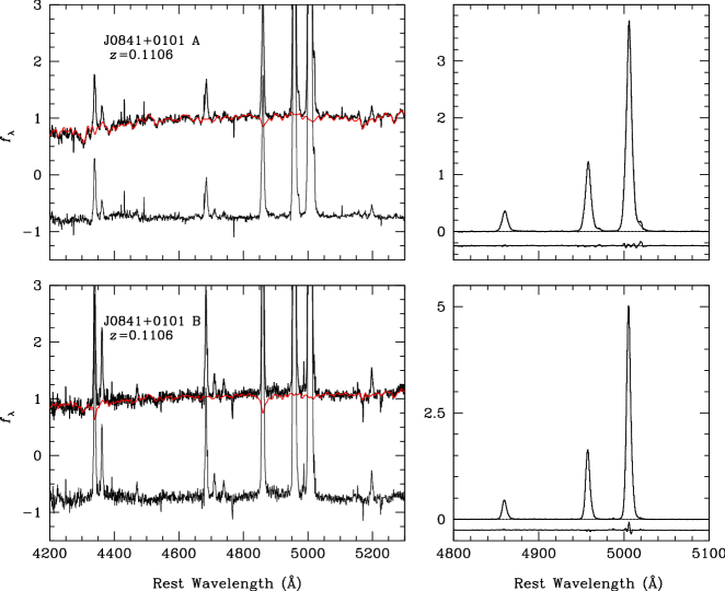
Figure 5: The binary narrow-line quasar serendipitously discovered in our spectroscopic campaign. Component A was observed by the SDSS and is the more massive of the two systems. Left: Stellar velocity dispersion fits using the best weighted fit of an F2, K1, and K4 star. These fits provide both a measurements of $\sigma_{\ast}$ and also a continuum subtraction. Flux densities are normalized to the continuum. Right: Fits to the H$\beta$ and [O III] emission lines using multi-component Gaussians; see text for details.

6 Discussion & Summary

We are looking for direct signs of feedback in the two-dimensional spatial extents and kinematics of the NLRs of a sample of luminous obscured active galaxies. Our conclusions are mixed. On the one hand, we see clear evidence that the AGN is stirring up the galaxy ISM. On the other hand, we do not see signs of galaxy-scale winds at high velocities. However, as we argue below, perhaps this is unsurprising.

We see two distinct signatures of a luminous accreting BH on the ionized gas in these galaxies. The NLRs are much more extended at these high luminosities than in lower-luminosity Seyfert galaxies. In fact, the AGNs are effectively photoionizing gas throughout the entire galaxy. This alone means that the AGN is heating the ISM on galaxy-wide scales. The impact of the AGN is more directly seen in the kinematics. We see very few ordered radial velocity curves; instead the velocity distributions are typically quite flat even at large radius. Perhaps even more striking is that the gas velocity dispersions are high out to large radius. As we have argued, not only do inactive galaxies uniformly show a drop in gas (and stellar) velocity dispersion at large radius, but even in ultra-luminous infrared galaxies the gas velocity dispersions are observed to drop at large radius. We cannot therefore attribute the gas stirring to gravitational effects such as mergers. It is most natural to implicate the accreting BH.

On the other hand, overall the velocities we observe in the NLR gas are not very high (a few hundred km s^-1). Taken at face value, our crude estimates suggest that very little of the ISM is moving fast enough to escape the galaxy, although a clumpy NLR complicates our ability to estimate this fraction robustly. In only one case do we see the spectacular outflowing nebulosity one might imagine in thinking of AGN feedback (SDSS J1356+1026). Before we can rule out that any gas is unbound from these galaxies, however, we should consider the impact of projection effects, potential observational biases, and some theoretical expectations.

Our observations suggest that ionized gas is ubiquitous within the galaxy but rare at larger (e.g., 10 kpc) scales. As explained above, the observed ratio of obscured to unobscured objects leads us to assume an ionization cone opening angle of $\sim 120\arcdeg$. With such a large opening angle, we would expect our slit to intercept the NLR nearly all the time, as we observe. On the other hand, we see extended gas on 10 kpc scales in only one case. Furthermore, the HST continuum images show extended emission on these large scales, but with a much smaller opening angle of 20-60°. Similarly, we have visually inspected the most luminous obscured AGNs from the Reyes et al. sample with $0.16<z<0.3$ and found evidence for small opening angles from the broad-band images (which have significant [O III] light in the $r$ band). Probably we are seeing the effects of surface brightness dimming at the outer reaches of the bicone. Although the true opening angle is large (120°), only a much narrower inner cone can be observed at 10 kpc. Taking the smaller opening angles, we expect to see extra-galactic extended gas only 20-40% of the time. That fraction is not inconsistent with the number of objects that we observe with emission line regions extending beyond their host galaxies.

Projection effects also preferentially bias us against detecting the true outflowing velocities. These are obscured objects, and on large scales we see evidence for ionization cones in the HST continuum imaging. We thus expect the largest accelerations to occur in the plane of the sky. We perform a Monte Carlo simulation in which the NLR is modeled as a biconical outflow with constant velocity as a function of radius, assuming different opening angles for the bicone (Fig. 6). We sample random lines of sight outside of the bicone, and find that while the intrinsic velocity is uniformly high, we only expect to observe high (e.g., approaching escape) velocities a small fraction of the time.

These simulations take into account only the bias introduced by projection effects and assume constant velocity and uniform emissivity within the bi-cone. We also considered more realistic models, in which velocity varies as a function of distance ($-2<d\log v/d\log r<1$) from the center, mass conservation is satisfied and the emissivity correspondingly declines as $n^{2}(r)$. Due to the decline of emissivity in these models, at a projected distance $d$ from the center the observed brightness is dominated by the location physically closest to the center (that is, $r=d$), and this gas is moving exactly in the plane of the sky exacerbating the projection bias. In the case $v(r)\propto r^{-2}$ the emissivity may be uniform, but the integral along the line of sight is dominated by gas that moves slower than the gas at $d$ because of the declining velocity profile. Therefore, in these more realistic situations we find a radial velocity distribution that is more peaked at zero than shown in Fig. 6. Thus, while we observe small escaping fractions, once projection effects are accounted for, the observations may be consistent with high velocities in a large fraction of the gas.

Finally, there is the possibility that the outflows operate predominantly on small scales. In local low-luminosity sources outflows are observed only within the inner hundreds of pc (e.g., Crenshaw & Kraemer, 2000). In addition, recent simulations by Debuhr et al. (2010) suggest that BHs do self-regulate their own growth but do not generate galaxy-wide outflows.

Figure 6: To illustrate the magnitude of the projection effects, we present the results of two Monte Carlo simulations of observed velocity distributions for a conical outflow with an opening angle of 60° (solid histogram) and 120° (dotted histogram). The line of sight is constrained to fall outside of the cone but is otherwise drawn from the appropriate random probability function. The outflow is assumed to emit uniformly and to have a constant outflow velocity $v_{\rm actual}$, but we measure the (smaller) radial velocity $v_{\rm obs}$. On the left, we show the distribution of velocities from both bicones, while on the right we show only the approaching bicone. Because many of the streamlines of the gas lie close to the plane of the sky, the observed velocities are biased to be significantly smaller than the real ones. This figure demonstrates that even if we detect only a small fraction of the gas at high velocities approaching the escape speed, a large fraction of the gas may actually be escaping.

Of course, other factors may be at play as well. There is the possibility that some fraction of the ionizing photons have escaped the galaxy (e.g., Netzer et al., 2004), or even that we are seeing galaxies in some pre-outburst phase, as may be expected if obscured accretion tends to accompany the late stages of merging and star formation activity (e.g., Mihos & Hernquist, 1994; Sanders & Mirabel, 1996; Canalizo & Stockton, 2001).

It is interesting to compare with simulations of galaxy-scale outflows. We start with the work of Proga et al. (2008) (see also Proga, 2007; Kurosawa & Proga, 2009). These simulations focus on smaller scales than those we probe, extending no further than 10 pc. However, it is at least a starting point for comparison. The simulations include radiative heating by both an accretion disk and an X-ray corona, and look at the impact of varying the density and temperature structure, as well as rotation, of the gas. We highlight a few generic conclusions from their studies that are very relevant to our work. First of all, the final flow includes both an equatorial inflow and a bipolar outflow. Consistent with our work, the opening angle of the outflowing cone can be quite wide (up to 160°). Also interesting to note is that the outflows can be dynamic, clumpy as we observe, and with multiple temperatures (ranging from the 10⁴ K gas observed here all the way to X-ray emitting temperatures). It remains to be seen whether the outflows on pc scales will propogate to larger (galaxy-wide scales).

A recent study by Hopkins et al. (in preparation) of outflows driven by AGNs in numerical simulations demonstrates several surprising similarities to the kinematics of the ionized gas we see in our study. The observations suggest that outflows are clumpy because the measurements of rms density and the mean density are highly discrepant. The simulations suggest that outflows are clumpy because they are subject to Rayleigh-Taylor instabilities. Furthermore, the rate of the decline of mean density with distance from the center seen in scattering observations is similar to that seen in numerical simulations where the motion of the gas becomes ballistic at large distances. The masses and the velocities of the outflows that we find are quite similar to those seen in numerical simulations, and although the kinetic energies of the outflows ($\sim 10^{42}$ erg s^-1) are just a small fraction of the total energy output of the AGN, the simulations suggest that the wind is in fact driven by a much stronger coupling of the AGN output to the gas. The small kinetic energies that we see at this late ($\sim 10^{7}$ years) stage are simply left-overs after much of the energy was efficiently radiated by the outflow. While these qualitative similarities are very encouraging, the specific mechanism responsible for coupling of the black hole output to the gas on much smaller spatial scales (which then develops into the relic outflow we see now) remains unidentified.

In short, it is clear that the presence of the AGN at the galaxy center impacts the entire galaxy. Whether significant mass outflows are driven, particularly in the radio-quiet regime considered here, remains an open question. The next step for this type of analysis is already underway. Integral-field unit observations (e.g., Villar-Martín et al., 2010), particularly with a wider wavelength coverage, will remove some of the ambiguities we struggle with.

This appendix includes all of the two-dimensional information for all galaxies that are spatially resolved in our observations (Figs. 12-20). Note in particular the high velocities and dispersions at large radius.

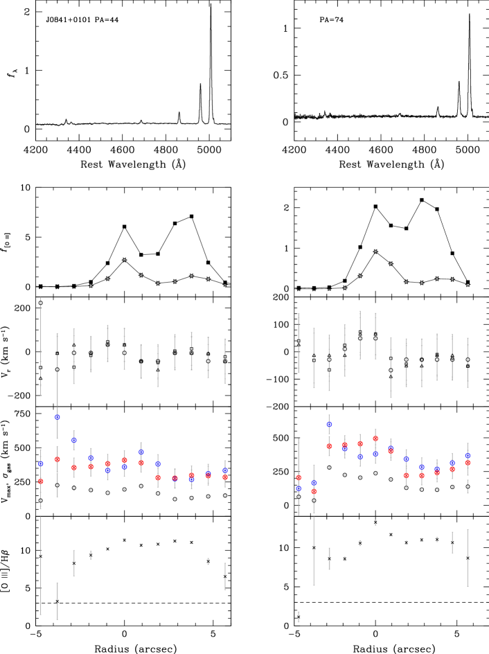
Figure 7: Resolved spectroscopic measurements for SDSS J0841+0101. In the top panel we show the central spectrum, extracted within the inner $\sim 1\arcsec$ arbitrarily normalized. The next panel shows the flux in the [O III] line (filled black squares) and in the continuum (open stars) as a function of radius (10^-15 erg cm^-2 s^-1). The velocity panel shows the velocity offset between [O III] and the “systemic” velocity as measured from H$\beta$ in the nuclear spectrum (filled black circles), the velocity dispersion in the gas (open black circles), and the maximum velocity (measured at $20\%$ of the line maximum) to the red (red open circle with cross) and to the blue (blue open circle with dot). Finally, the ratio of [O III]/H$\beta$ is plotted (black crosses). A ratio of [O III]/H$\beta$ of three is noted with the dashed line.

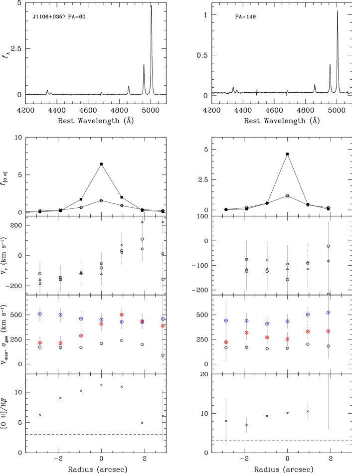
Figure 8: Resolved spectroscopic measurements for SDSS J1106+0357. Symbols as above.

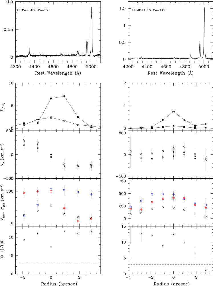
Figure 9: Resolved spectroscopic measurements for SDSS J1124+0456 and SDSS J1142+1027. Symbols as above.

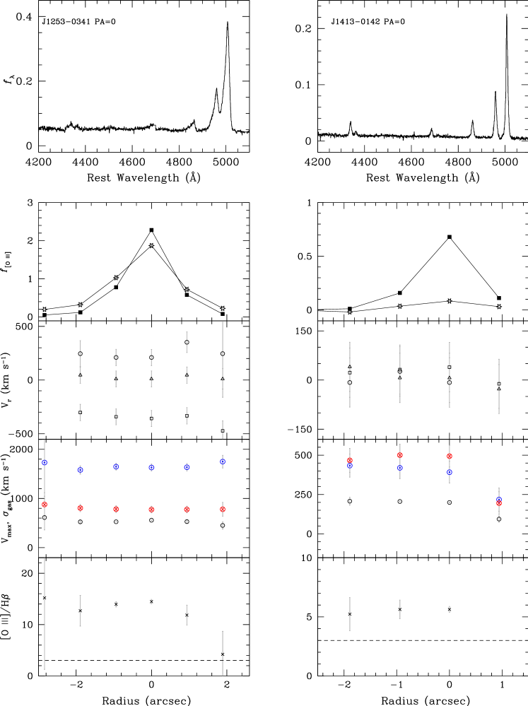
Figure 10: Resolved spectroscopic measurements for SDSS J1253$-0341$ and SDSS J1413$-0142$. Symbols as above.

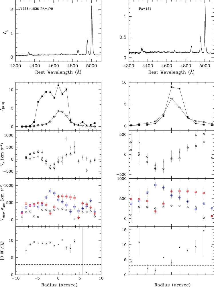
Figure 11: Resolved spectroscopic measurements for SDSS J1356+1026. Symbols as above, shown for each slit position.

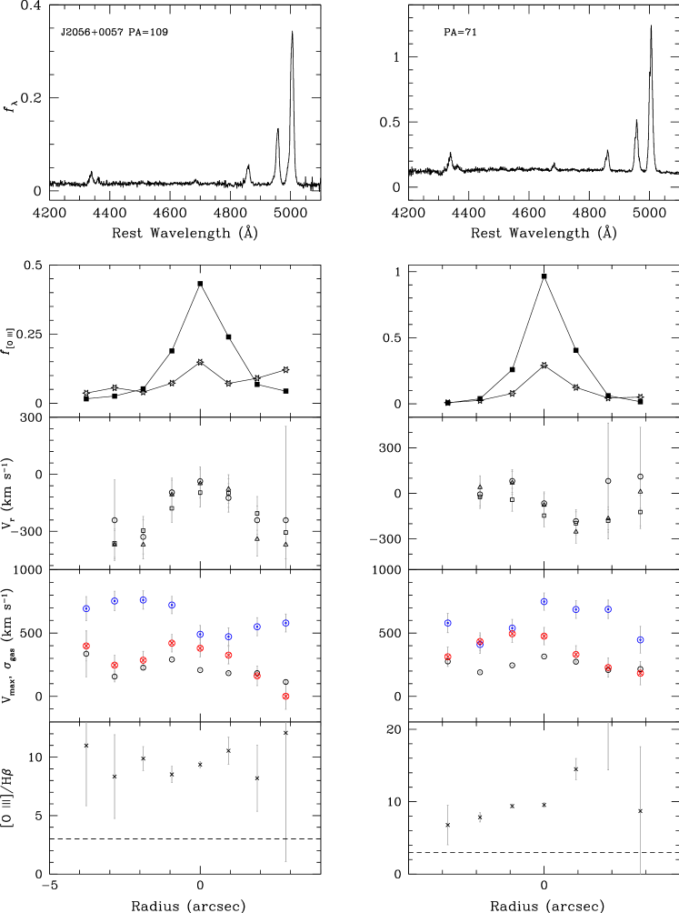
Figure 12: Resolved spectroscopic measurements for SDSS J2056+0057. Symbols as above, shown for each slit position.

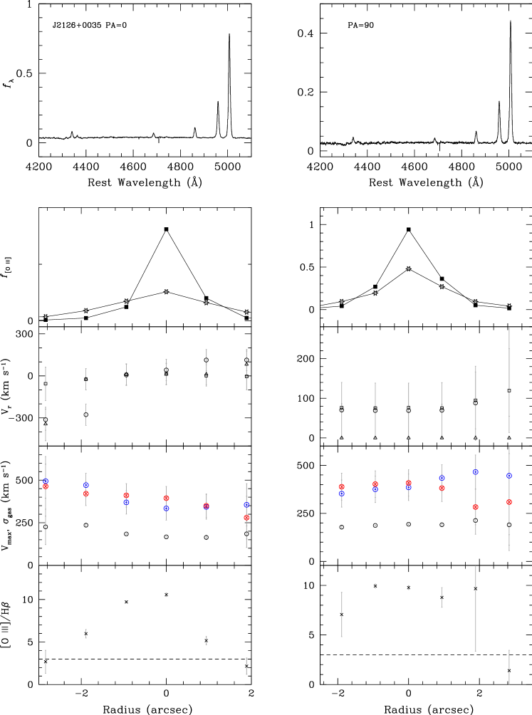
Figure 13: Resolved spectroscopic measurements for SDSS J2126+0035. Symbols as above, shown for each slit position.

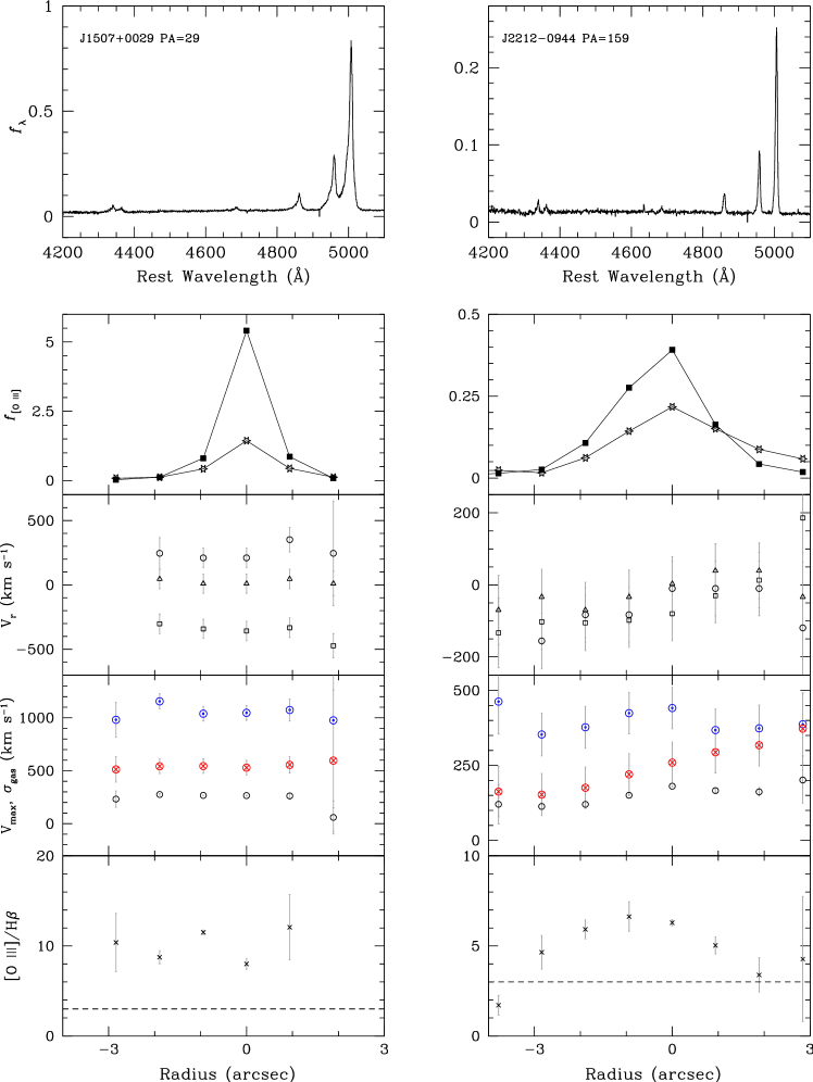
Figure 14: Resolved spectroscopic measurements for SDSS J1507+0029 and SDSS J2212$-0944$. Symbols as above.

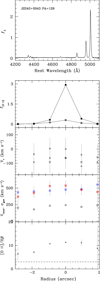
Figure 15: Resolved spectroscopic measurements for SDSS J2240+0043. Symbols as above.

References

- Allington-Smith et al. (1994) Allington-Smith, J., et al. 1994, PASP, 106, 983
- Barbosa et al. (2009) Barbosa, F. K. B., Storchi-Bergmann, T., Cid Fernandes, R., Winge, C., & Schmitt, H. 2009, MNRAS, 396, 2
- Barth et al. (2008) Barth, A. J., Bentz, M. C., Greene, J. E., & Ho, L. C. 2008, ApJ, 683, L119
- Becker et al. (1995) Becker, R. H., White, R. L., & Helfand, D. J. 1995, ApJ, 450, 559
- Bennert et al. (2002) Bennert, N., Falcke, H., Schulz, H., Wilson, A. S., & Wills, B. J. 2002, ApJ, 574, L105
- Bennert et al. (2006) Bennert, N., Jungwiert, B., Komossa, S., Haas, M., & Chini, R. 2006, A&A, 456, 953
- Bertola et al. (1995) Bertola, F., Cinzano, P., Corsini, E. M., Rix, H., & Zeilinger, W. W. 1995, ApJ, 448, L13
- Best et al. (2005) Best, P. N., Kauffmann, G., Heckman, T. M., Brinchmann, J., Charlot, S., Ivezić, Ž., & White, S. D. M. 2005, MNRAS, 362, 25
- Bîrzan et al. (2004) Bîrzan, L., Rafferty, D. A., McNamara, B. R., Wise, M. W., & Nulsen, P. E. J. 2004, ApJ, 607, 800
- Boksenberg et al. (1995) Boksenberg, A., et al. 1995, ApJ, 440, 151
- Canalizo & Stockton (2001) Canalizo, G., & Stockton, A. 2001, ApJ, 555, 719
- Colbert et al. (1996) Colbert, E. J. M., Baum, S. A., Gallimore, J. F., O’Dea, C. P., Lehnert, M. D., Tsvetanov, Z. I., Mulchaey, J. S., & Caganoff, S. 1996, ApJS, 105, 75
- Colina et al. (2005) Colina, L., Arribas, S., & Monreal-Ibero, A. 2005, ApJ, 621, 725
- Comerford et al. (2009a) Comerford, J. M., Griffith, R. L., Gerke, B. F., Cooper, M. C., Newman, J. A., Davis, M., & Stern, D. 2009a, ApJ, 702, L82
- Comerford et al. (2009b) Comerford, J. M., et al. 2009b, ApJ, 698, 956
- Condon et al. (1998) Condon, J. J., Cotton, W. D., Greisen, E. W., Yin, Q. F., Perley, R. A., Taylor, G. B., & Broderick, J. J. 1998, AJ, 115, 1693
- Conroy & Ostriker (2008) Conroy, C., & Ostriker, J. P. 2008, ApJ, 681, 151
- Crenshaw & Kraemer (2000) Crenshaw, D. M., & Kraemer, S. B. 2000, ApJ, 532, L101
- Crenshaw et al. (2003) Crenshaw, D. M., Kraemer, S. B., & George, I. M. 2003, ARA&A, 41, 117
- Crenshaw et al. (2000) Crenshaw, D. M., et al. 2000, AJ, 120, 1731
- Croton et al. (2006) Croton, D. J., et al. 2006, MNRAS, 365, 11
- Debuhr et al. (2010) Debuhr, J., Quataert, E., Ma, C., & Hopkins, P. 2010, MNRAS, 406, L55
- Draine (2003) Draine, B. T. 2003, ApJ, 598, 1017
- Evans et al. (1993) Evans, I. N., Tsvetanov, Z., Kriss, G. A., Ford, H. C., Caganoff, S., & Koratkar, A. P. 1993, ApJ, 417, 82
- Feigelson & Nelson (1985) Feigelson, E. D., & Nelson, P. I. 1985, ApJ, 293, 192
- Fillmore et al. (1986) Fillmore, J. A., Boroson, T. A., & Dressler, A. 1986, ApJ, 302, 208
- Fraquelli et al. (2003) Fraquelli, H. A., Storchi-Bergmann, T., & Levenson, N. A. 2003, MNRAS, 341, 449
- Fu et al. (2010) Fu, H., Myers, A. D., Djorgovski, S. G., & Yan, L. 2010, submitted to ApJL (arXiv/1009.0767)
- Fu & Stockton (2009) Fu, H., & Stockton, A. 2009, ApJ, 690, 953
- Gallagher et al. (2007) Gallagher, S. C., Hines, D. C., Blaylock, M., Priddey, R. S., Brandt, W. N., & Egami, E. E. 2007, ApJ, 665, 157
- Gerke et al. (2007) Gerke, B. F., et al. 2007, ApJ, 660, L23
- Greene & Ho (2005) Greene, J. E., & Ho, L. C. 2005, ApJ, 627, 721
- Greene et al. (2009) Greene, J. E., Zakamska, N. L., Liu, X., Barth, A. J., & Ho, L. C. 2009, ApJ, 702, 441
- Groves et al. (2004) Groves, B. A., Cecil, G., Ferruit, P., & Dopita, M. A. 2004, ApJ, 611, 786
- Gültekin et al. (2009) Gültekin, K., et al. 2009, ApJ, 698, 198
- Hamilton & Keel (1987) Hamilton, D., & Keel, W. C. 1987, ApJ, 321, 211
- Häring & Rix (2004) Häring, N., & Rix, H. 2004, ApJ, 604, L89
- Heinz et al. (2006) Heinz, S., Brüggen, M., Young, A., & Levesque, E. 2006, MNRAS, 373, L65
- Ho (2009) Ho, L. C. 2009, ApJ, accepted
- Ho et al. (1997) Ho, L. C., Filippenko, A. V., Sargent, W. L. W., & Peng, C. Y. 1997, ApJS, 112, 391
- Hopkins et al. (2006) Hopkins, P. F., Hernquist, L., Cox, T. J., Di Matteo, T., Robertson, B., & Springel, V. 2006, ApJS, 163, 1
- Humphrey et al. (2010) Humphrey, A., Villar-Martín, M., Sánchez, S. F., Martínez-Sansigre, A., González Delgado, R., Pérez, E., Tadhunter, C., & Pérez-Torres, M. A. 2010, MNRAS, L113
- Husemann et al. (2008) Husemann, B., Wisotzki, L., Sánchez, S. F., & Jahnke, K. 2008, A&A, 488, 145
- Isobe et al. (1986) Isobe, T., Feigelson, E. D., & Nelson, P. I. 1986, ApJ, 306, 490
- Jorgensen et al. (1995) Jorgensen, I., Franx, M., & Kjaergaard, P. 1995, MNRAS, 276, 1341
- Kurosawa & Proga (2009) Kurosawa, R., & Proga, D. 2009, MNRAS, 397, 1791
- Lal & Ho (2010) Lal, D. V., & Ho, L. C. 2010, AJ, 139, 1089
- Liu et al. (2010a) Liu, X., Greene, J. E., Shen, Y., & Strauss, M. A. 2010a, ApJ, 715, L30
- Liu et al. (2010b) Liu, X., Shen, Y., Strauss, M. A., & Greene, J. E. 2010b, ApJ, 708, 427
- Liu et al. (2009) Liu, X., Zakamska, N. L., Greene, J. E., Strauss, M. A., Krolik, J. H., & Heckman, T. M. 2009, ApJ, 702, 1098
- Matheson et al. (2008) Matheson, T., et al. 2008, AJ, 135, 1598
- McCarthy (1993) McCarthy, P. J. 1993, ARA&A, 31, 639
- McNamara & Nulsen (2007) McNamara, B. R., & Nulsen, P. E. J. 2007, ARA&A, 45, 117
- Meléndez et al. (2008) Meléndez, M., et al. 2008, ApJ, 682, 94
- Mihos & Hernquist (1994) Mihos, J. C., & Hernquist, L. 1994, ApJ, 431, L9
- Moe et al. (2009) Moe, M., Arav, N., Bautista, M. A., & Korista, K. T. 2009, ApJ, 706, 525
- Mulchaey et al. (1996a) Mulchaey, J. S., Wilson, A. S., & Tsvetanov, Z. 1996a, ApJS, 102, 309
- Mulchaey et al. (1996b) —. 1996b, ApJ, 467, 197
- Nelson & Whittle (1996) Nelson, C. H., & Whittle, M. 1996, ApJ, 465, 96
- Nesvadba et al. (2008) Nesvadba, N. P. H., Lehnert, M. D., De Breuck, C., Gilbert, A. M., & van Breugel, W. 2008, A&A, 491, 407
- Nesvadba et al. (2006) Nesvadba, N. P. H., Lehnert, M. D., Eisenhauer, F., Gilbert, A., Tecza, M., & Abuter, R. 2006, ApJ, 650, 693
- Netzer et al. (2004) Netzer, H., Shemmer, O., Maiolino, R., Oliva, E., Croom, S., Corbett, E., & di Fabrizio, L. 2004, ApJ, 614, 558
- Parrish et al. (2009) Parrish, I. J., Quataert, E., & Sharma, P. 2009, ApJ, 703, 96
- Pizzella et al. (2004) Pizzella, A., Corsini, E. M., Vega Beltrán, J. C., & Bertola, F. 2004, A&A, 424, 447
- Pogge (1988) Pogge, R. W. 1988, ApJ, 328, 519
- Proga (2007) Proga, D. 2007, ApJ, 661, 693
- Proga & Kallman (2004) Proga, D., & Kallman, T. R. 2004, ApJ, 616, 688
- Proga et al. (2008) Proga, D., Ostriker, J. P., & Kurosawa, R. 2008, ApJ, 676, 101
- Ptak et al. (2006) Ptak, A., Zakamska, N. L., Strauss, M. A., Krolik, J. H., Heckman, T. M., Schneider, D. P., & Brinkmann, J. 2006, ApJ, 637, 147
- Reichard et al. (2003) Reichard, T. A., et al. 2003, AJ, 125, 1711
- Reyes et al. (2008) Reyes, R., Zakamska, N. L., Strauss, M. A., Green, J., Krolik, J. H., Shen, Y., Richards, G. T., Anderson, S. F., & Schneider, D. P. 2008, AJ, 136, 2373
- Ruiz et al. (2001) Ruiz, J. R., et al. 2001, AJ, 122, 2961
- Rupke et al. (2002) Rupke, D. S., Veilleux, S., & Sanders, D. B. 2002, ApJ, 570, 588
- Rupke et al. (2005) —. 2005, ApJ, 632, 751
- Salviander et al. (2007) Salviander, S., Shields, G. A., Gebhardt, K., & Bonning, E. W. 2007, ApJ, 662, 131
- Sanders & Mirabel (1996) Sanders, D. B., & Mirabel, I. F. 1996, ARA&A, 34, 749
- Schmidt et al. (2007) Schmidt, G. D., Smith, P. S., Hines, D. C., Tremonti, C. A., & Low, F. J. 2007, ApJ, 666, 784
- Schmitt et al. (2003) Schmitt, H. R., Donley, J. L., Antonucci, R. R. J., Hutchings, J. B., Kinney, A. L., & Pringle, J. E. 2003, ApJ, 597, 768
- Shen et al. (2008) Shen, Y., Strauss, M. A., Hall, P. B., Schneider, D. P., York, D. G., & Bahcall, N. A. 2008, ApJ, 677, 858
- Shields et al. (2003) Shields, G. A., Gebhardt, K., Salviander, S., Wills, B. J., Xie, B., Brotherton, M. S., Yuan, J., & Dietrich, M. 2003, ApJ, 583, 124
- Sijacki et al. (2008) Sijacki, D., Pfrommer, C., Springel, V., & Enßlin, T. A. 2008, MNRAS, 387, 1403
- Silk & Rees (1998) Silk, J., & Rees, M. J. 1998, A&A, 331, L1
- Sironi & Socrates (2010) Sironi, L., & Socrates, A. 2010, ApJ, 710, 891
- Smith et al. (2010) Smith, K. L., Shields, G. A., Bonning, E. W., McMullen, C. C., Rosario, D. J., & Salviander, S. 2010, ApJ, 716, 866
- Sołtan (1982) Sołtan, A. 1982, MNRAS, 200, 115
- Springel et al. (2005) Springel, V., Di Matteo, T., & Hernquist, L. 2005, MNRAS, 361, 776
- Stockton et al. (2006) Stockton, A., Fu, H., Henry, J. P., & Canalizo, G. 2006, ApJ, 638, 635
- Stockton & MacKenty (1987) Stockton, A., & MacKenty, J. W. 1987, ApJ, 316, 584
- Storchi-Bergmann et al. (1992) Storchi-Bergmann, T., Wilson, A. S., & Baldwin, J. A. 1992, ApJ, 396, 45
- Tabor & Binney (1993) Tabor, G., & Binney, J. 1993, MNRAS, 263, 323
- Tadhunter & Tsvetanov (1989) Tadhunter, C., & Tsvetanov, Z. 1989, Nature, 341, 422
- Tadhunter (1991) Tadhunter, C. N. 1991, MNRAS, 251, 46P
- Tchekhovskoy et al. (2010) Tchekhovskoy, A., Narayan, R., & McKinney, J. C. 2010, ApJ, 711, 50
- Thoul & Weinberg (1995) Thoul, A. A., & Weinberg, D. H. 1995, ApJ, 442, 480
- Tremonti et al. (2007) Tremonti, C. A., Moustakas, J., & Diamond-Stanic, A. M. 2007, ApJ, 663, L77
- Unger et al. (1987) Unger, S. W., Pedlar, A., Axon, D. J., Whittle, M., Meurs, E. J. A., & Ward, M. J. 1987, MNRAS, 228, 671
- van Breugel et al. (1986) van Breugel, W. J. M., Heckman, T. M., Miley, G. K., & Filippenko, A. V. 1986, ApJ, 311, 58
- van Dokkum (2001) van Dokkum, P. G. 2001, PASP, 113, 1420
- Vega Beltrán et al. (2001) Vega Beltrán, J. C., Pizzella, A., Corsini, E. M., Funes, J. G., Zeilinger, W. W., Beckman, J. E., & Bertola, F. 2001, A&A, 374, 394
- Veilleux et al. (2005) Veilleux, S., Cecil, G., & Bland-Hawthorn, J. 2005, ARA&A, 43, 769
- Veilleux et al. (2003) Veilleux, S., Shopbell, P. L., Rupke, D. S., Bland-Hawthorn, J., & Cecil, G. 2003, AJ, 126, 2185
- Vignali et al. (2010) Vignali, C., Alexander, D. M., Gilli, R., & Pozzi, F. 2010, MNRAS, 404, 48
- Villar-Martín et al. (1999) Villar-Martín, M., Tadhunter, C., Morganti, R., Axon, D., & Koekemoer, A. 1999, MNRAS, 307, 24
- Villar-Martín et al. (2010) Villar-Martín, M., Tadhunter, C., Pérez, E., Humphrey, A., Martínez-Sansigre, A., Delgado, R. G., & Pérez-Torres, M. 2010, MNRAS, 407, L6
- Walsh et al. (2008) Walsh, J. L., Barth, A. J., Ho, L. C., Filippenko, A. V., Rix, H.-W., Shields, J. C., Sarzi, M., & Sargent, W. L. W. 2008, AJ, 136, 1677
- Wang et al. (2009) Wang, J., Chen, Y., Hu, C., Mao, W., Zhang, S., & Bian, W. 2009, ApJ, 705, L76
- Weymann et al. (1981) Weymann, R. J., Carswell, R. F., & Smith, M. G. 1981, ARA&A, 19, 41
- Whittle (1992a) Whittle, M. 1992a, ApJS, 79, 49
- Whittle (1992b) —. 1992b, ApJ, 387, 121
- Xu et al. (1999) Xu, C., Livio, M., & Baum, S. 1999, AJ, 118, 1169
- Yee (1980) Yee, H. K. C. 1980, ApJ, 241, 894
- York et al. (2000) York, D. G., et al. 2000, AJ, 120, 1579
- Yu & Tremaine (2002) Yu, Q., & Tremaine, S. 2002, MNRAS, 335, 965
- Zakamska et al. (2008) Zakamska, N. L., Gómez, L., Strauss, M. A., & Krolik, J. H. 2008, AJ, 136, 1607
- Zakamska & Narayan (2003) Zakamska, N. L., & Narayan, R. 2003, ApJ, 582, 162
- Zakamska et al. (2004) Zakamska, N. L., Strauss, M. A., Heckman, T. M., Ivezić, Ž., & Krolik, J. H. 2004, AJ, 128, 1002
- Zakamska et al. (2003) Zakamska, N. L., et al. 2003, AJ, 126, 2125
- Zakamska et al. (2005) —. 2005, AJ, 129, 1212
- Zakamska et al. (2006) —. 2006, AJ, 132, 1496