Physical and radiative properties of the first core accretion shock

Abstract

Context. Radiative shocks play a dominant role in star formation. The accretion shocks on the first and second Larson’s cores involve radiative processes and are thus characteristic of radiative shocks.

Aims. In this study, we explore the formation of the first Larson’s core and characterize the radiative and dynamical properties of the accretion shock, using both analytical and numerical approaches.

Methods. We develop both numerical radiation-hydrodynamics calculations and a semi-analytical model that characterize radiative shocks in various physical conditions, for radiating or barotropic fluids. Then, we perform 1D spherical collapse calculations of the first Larson’s core, using a grey approximation for the opacity of the material. We consider three different models for radiative transfer, namely: the barotropic approximation, the flux limited diffusion approximation and the more complete M1 model. We investigate the characteristic properties of the collapse and of the first core formation. Comparison between the numerical results and our semi-analytical model for radiative shocks shows that this latter reproduces quite well the core properties obtained with the numerical calculations.

Results. The accretion shock on the first Larson core is found to be supercritical, i.e. the post and pre-shock temperatures are equal, implying that all the accretion shock energy on the core is radiated away. The shock properties are well described by the semi-analytical model. The flux limited diffusion approximation is found to agree quite well with the results based on the M1 model of radiative transfer, and is thus appropriate to study the star formation process. In contrast, the barotropic approximation does not correctly describe the thermal properties of the gas during the collapse.

Conclusions. We have explored and characterized the properties of radiative shocks typical of the formation of the first Larson’s core during protostellar collapse, using both radiation-hydrodynamics numerical simulations and a semi-analytical model, except, for this latter, in the case of subcritical shocks in an optically thin medium. We show that a consistent treatment of radiation and hydrodynamics is mandatory to correctly handle the cooling of the gas during the core formation and thus to obtain the correct mechanical and thermal properties for this latter. We show that the flux limited diffusion approximation is appropriate to perform star formation calculations and thus allows a tractable and relatively correct treatment of radiative transfer in multidimensional radiation-hydrodynamics calculations.

1 Introduction

Star formation involves a large variety of complex physical processes. Among them, radiative transfer appears to be one of the most important ones, since it governs the behaviour of the earliest phases of the collapse and the formation of the so-called first core (Larson, 1969). It is well established that the molecular gas experiences different thermal regimes, from isothermal to adiabatic, during the earliest phase of the collapse, via the coupling between gas, dust and radiation (e.g. Larson, 1969; Tscharnuter & Winkler, 1979; Masunaga et al., 1998).

Since the pioneering works of Winkler & Newman and Tscharnuter (Winkler & Newman, 1980; Tscharnuter, 1987), relatively few studies have been devoted to the accretion shock on the first Larson’s core. This shock is a radiative shock, i.e. radiation can escape from the infalling material. Once this infalling gas has been shocked and has reached an optical depth of $\leavevmode\nobreak\ 1$, it becomes more or less adiabatic, at a given entropy level characteristic of the first core initial energy content. This entropy content is kept roughly constant during the nearly adiabatic subsequent stages of the collapse and the formation of the second core. The accretion shock on the first core is thus of prime importance, since it determines the entropy level of the following stages of star formation, up to the formation of the protostar itself.

A radiative shock is a shock that is so strong that it emits radiation which in turn affects the hydrodynamic behaviour of the flow. The equations of radiation-hydrodynamics (RHD) must thus be solved consistently to properly explore this kind of a process. Radiative shocks are common in astrophysics, e.g. in star formation regions or around supernovae remnants. They are well studied in the literature, from the theoretical, experimental and numerical points of view (e.g. Bouquet et al., 2000; Drake, 2007; González et al., 2009). The large variety of radiative shocks makes it difficult to try to classify them (Drake, 2005; Michaut et al., 2009).

In this work, we study radiative shocks from both numerically and analytically. We focus on the properties of the accretion shock during the formation of the first prestellar core. In the first part of the paper, we recall the main properties of radiative shocks. Then, considering the jump relations for a radiating fluid, we focus on some particular kinds of radiative shocks, with upstream and downstream material characterized by different optical depth properties. We also consider the case of a shock taking place in a barotropic material, since the barotropic approximation is the simplest way to characterize the thermal evolution of the gas during the collapse (e.g. Commerçon et al., 2008).

In the second part of this work, we study the impact of various models of radiative transfer on the protostellar collapse. Radiation hydrodynamics plays here a crucial role, for instance by evacuating the compressional energy, leading to a nearly isothermal free-fall collapse phase. Radiation transfer also has a dramatic impact on the accretion shock, with the infalling gas kinetic energy being either converted into internal energy in the static adiabatic core or radiated away. This ratio between the energy accreted onto the star and the one radiated away is a key quantity, as it ultimately determines the entropy content of the forming star. Using a 1D spherical code, we compare results of calculations done with a barotropic EOS, a flux limited diffusion approximation, and a M1 model for radiative transfer, assuming grey opacity for the infalling material. 1D calculations retain the important virtue of allowing detailed and complex physical processes to be considered in dense core collapse calculations, which is not the case in a multidimensional approach. In consequence, a 1D approach enables us to characterize the impact of these various physical processes on the results, allowing a better characterization of the validity of simplified multidimensional studies (e.g. Commerçon et al., 2010, 2011).

This paper is organized as follows. In the first section, we recall the basic properties of radiative shocks and develop semi-analytical models that can be applied in some particular cases for a radiating fluid and a barotropic fluid. In Sect. 3, we detail the numerical method and the physics inputs used in our calculations. In Sect. 4, we derive the first Larson’s core properties from the numerical calculations, using various approximations for the radiative transfer, and compare the results with the ones obtained by Masunaga et al. (1998). We also present an original semi-analytical model that allows a simple interpretation of the numerical results. Eventually, Sect. 5 summarizes our main results.

2 Radiative shock - A semi-analytic model

2.1 A qualitative picture of radiative shocks

Depending on the shock’s strength, radiative shocks belong to two groups: the subcritical shocks and the supercritical shocks. As the strength of a shock increases, the postshock temperature $T_{2}$ rises, producing a radiative flux of order $\sigma T_{2}^{4}$ that increases very rapidly. This flux penetrates the upstream material and preheats this latter to a temperature $T_{-}$ immediately ahead of the shock front (radiative precursor) that is proportional to the incident flux. $T_{-}$ increases rapidly with the shock strength and eventually becomes equal to $T_{2}$. A shock with $T_{-}<T_{2}$ is called a subcritical shock. Because the material entering the shock is preheated, the postshock temperature $T_{+}$ exceeds its asymptotic equilibrium value $T_{2}$, and decays downstream as the material cools by emitting photons that propagate across the shock (see Fig. 1 for various shock characteristics).

For stringer shocks, the preheating becomes so important that the preshock temperature equals the postshock equilibrium temperature $T_{2}$. The shock velocity at which the postshock and preshock temperatures are equal, defines the critical shock. For higher shock velocities, $T_{-}$ cannot exceed $T_{2}$, the excess energy forces the radiative precursor further into the upstream region with a temperature close to $T_{2}$. Pre- and post-shock temperatures are equal, the supercritical shock is thus isothermal. Radiation and matter are still out of equilibrium in some part of the precursor, but come to equilibrium when temperature approaches $T_{2}$. The upstream kinetic energy is radiated at the shock.

Most of the early work on radiative shocks has been described in Zel’Dovich & Raizer (1967) and Mihalas & Mihalas (1984), where readers can find the basic equations of the front structure, radiative precursor extension, etc…

Figure 1: Temperature and density profiles in a subcritical shock (left) and a supercritical shock (right). Adapted from Zel’Dovich & Raizer (1967).

2.2 Jump relations for a radiating material

Consider the jump relations (Rankine Hugoniot) for a radiating flow (see Mihalas & Mihalas, 1984; Zel’Dovich & Raizer, 1967; Drake, 2007). Conservation of mass, momentum and energy yield

$$\rho_{1}u_{1} = \rho_{2}u_{2}\equiv\dot{m},$$ (1)

$$\rho_{1}u_{1}^{2}+P_{1}+P_{\mathrm{r1}} = \rho_{2}u_{2}^{2}+P_{2}+P_{\mathrm{r2}},$$ (2)

$$\dot{m}\left(h_{1}+\rho_{1}u_{1}^{2}\right)+F_{\mathrm{r1}}+u_{1}\left(E_{\mathrm{r1}}+P_{\mathrm{r1}}\right) =$$

$$\dot{m}\left(h_{2}+\rho_{2}u_{2}^{2}\right) + F_{\mathrm{r2}}+u_{2}\left(E_{\mathrm{r2}}+P_{\mathrm{r2}}\right),$$ (3)

where subscripts “1” and “2” denote respectively the upstream and downstream states, all radiation quantities are estimated in the comoving frame. $h$ corresponds to the gas specific enthalpy ($h=\epsilon+P/\rho$, with $e=\rho\epsilon=P/(\gamma-1)$) and $\dot{m}$ is the mass flux through the shock. In comparison with the hydrodynamical case, the pressure is now the total pressure, i.e. the gas plus radiation contributions, $P+P_{\mathrm{r}}$, and the specific enthalpy is the total specific enthalpy, $\epsilon+(P+P_{\mathrm{r}}+E_{\mathrm{r}})/\rho$. The radiation energy $E_{\mathrm{r}}$ and the radiation pressure $P_{\mathrm{r}}$ are important only at high temperatures or low densities, whereas the radiation flux, $F_{\mathrm{r}}$, plays a fundamental role in all radiative shocks.

Contrarily to the hydrodynamical case, the system of equations (1), (2) and (3) can not be solved explicitly. We need to make some assumptions on both the upstream and downstream materials. In what follows, we distinguish two cases: i) the upstream and downstream materials are opaque, ii) the upstream material is optically thin and the downstream material remains opaque.

2.2.1 Radiative shock in an optically thick medium

This is the most studied case (e.g. Mihalas & Mihalas, 1984; Drake, 2007). It occurs, for instance, in shocks in stellar interiors, where matter is both dense and hot. At a sufficiently large distance from the front, matter and radiation are in equilibrium and both the downstream and upstream materials are opaque ($F_{\mathrm{r1}}=F_{\mathrm{r2}}=0$). Any radiation crossing the front from the hot downstream material into the cool upstream material is reabsorbed in the radiative precursor, into which it propagates by diffusion. Outside this diffusion layer, the flux vanishes and we have

$$\small\dot{m}\left(h_{1}+\rho_{1}u_{1}^{2}\right)+u_{1}\left(E_{\mathrm{r1}}+P_{\mathrm{r1}}\right)=\dot{m}\left(h_{2}+\rho_{2}u_{2}^{2}\right)+u_{2}\left(E_{\mathrm{r2}}+P_{\mathrm{r2}}\right).$$ (4)

Since matter and radiation are in equilibrium and the material is opaque, we have $E_{\mathrm{r}}=3P_{\mathrm{r}}=a_{\mathrm{R}}T^{4}$. Defining the compression ratio $r=\rho_{2}/\rho_{1}=u_{1}/u_{2}$, we can rewrite equations (2) and (3) in the non-dimensional form

$$\gamma\mathcal{M}_{1}^{2}\left(\frac{r-1}{r}\right)=\left(\Pi-1\right)+\alpha_{1}\left(\left(\frac{\Pi}{r}\right)^{4}-1\right),$$ (5)

and

$$\frac{\gamma}{2}\mathcal{M}_{1}^{2}\left(\frac{r^{2}-1}{r^{2}}\right)=\frac{\gamma}{\gamma-1}\left(\frac{\Pi}{r}-1\right)+4\alpha_{1}\left(\frac{\Pi^{4}}{r^{5}}-1\right),$$ (6)

where $\Pi=P_{2}/P_{1}$, $\alpha_{1}=(1/3)a_{\mathrm{R}}T_{1}^{4}/P_{1}$ and $\mathcal{M}_{1}$ is the hydrodynamic Mach number, $\mathcal{M}_{1}=u_{1}/c_{s1}=u_{1}/(\gamma P_{1}/\rho_{1})^{1/2}$. The coupled equations (5) and (6) are solved numerically to get the variations of $\Pi$ and $r$ as function of $\mathcal{M}_{1}$ and $\alpha_{1}$.

The compression ratio rises from $r=4$ for a pure hydrodynamic shock with $\gamma=5/3$ to $r=7$, which corresponds to the limiting compression ratio for a gas with $\gamma=4/3$, i.e pure radiation, a gas made of photons. The stronger the shock, the greater the radiative effects, even for a very small initial ratio of radiative pressure to gas pressure. When the upstream radiative pressure increases, the shock becomes immediately radiative since radiative pressure increases as $T^{4}$, whereas the gas pressure increases only linearly with temperature. As shown in Mihalas & Mihalas (1984), for a strong radiating shock, since the compression ratio is fixed, the temperature ratio increases only as $\mathcal{M}_{1}^{1/2}$, whereas it rises as $\mathcal{M}_{1}^{2}$ in a non-radiating shock. Note that if $P_{\mathrm{r}}/P<10^{-5}$, the non-radiating fluid approximation becomes valid for an upstream Mach number $\mathcal{M}_{1}<10$.

2.2.2 Radiative shock with an optically thin upstream material

Suppose now that the shock is propagating in an optically thin material with an opaque downstream region, as in the case of star formation (e.g., Calvet & Gullbring, 1998). In the low mass star formation context, the radiative energy and pressure can be neglected compared to the gas internal energy for the first core accretion shock.

Let us consider the material and radiative quantities at the discontinuity, outside the spike in gas temperature (i.e., between regions with subscripts ”2” and ”-”). We have

$$\centering\rho_{-}u_{-}\@add@centering = \rho_{2}u_{2}\equiv\dot{m},$$ (7)

$$\rho_{-}u_{-}^{2}+P_{-} = \rho_{2}u_{2}^{2}+P_{2},$$ (8)

$$\dot{m}\left(h_{-}+\rho_{-}u_{-}^{2}\right) = \dot{m}\left(h_{2}+\rho_{2}u_{2}^{2}\right)+\Delta F_{\mathrm{r}},$$ (9)

where $\Delta F_{\mathrm{r}}=F_{\mathrm{r2}}-F_{\mathrm{r-}}$. We consider the case of a non zero net flux $|F_{\mathrm{r2}}-F_{\mathrm{r-}}|$ across the shock. The jump relations, derived from the conservation equations (1), (2) and (3), read

$$\frac{\rho_{2}}{\rho_{-}}=\frac{\left[(\gamma+1)P_{2}+(\gamma-1)P_{-}\right]u_{2}+2(\gamma-1)\Delta F_{\mathrm{r}}}{\left[(\gamma+1)P_{-}+(\gamma-1)P_{2}\right]u_{2}},$$ (10)

and

$$\frac{T_{2}}{T_{-}}=\left(\frac{P_{2}}{P_{-}}\right)\frac{\left[(\gamma+1)P_{-}+(\gamma-1)P_{2}\right]u_{-}-2(\gamma-1)\Delta F_{\mathrm{r}}}{\left[(\gamma+1)P_{2}+(\gamma-1)P_{-}\right]u_{-}}.$$ (11)

These two relations show that radiative energy transport (i.e. the radiative flux) across a shock can significantly alter the density, temperature and velocity profiles of the flow. Both upstream and downstream materials are affected over distances which depend on the material opacity. As mentioned before, the structure of a radiative shock is as follows: the upstream material is preheated by a radiation precursor while the downstream material is cooled by radiative losses.

As for the previous opaque case for which we use an iterative solver, the downstream quantities can not be derived analytically from the conservation relations for given upstream conditions. The radiative flux has to be known and the result depends on the upstream flow.

The simplest case to study is a supercritical shock, where $T_{-}=T_{2}$ and then $h_{-}=h_{2}$. Using the same adimensional parameters as for the opaque case, we have

$$\gamma\mathcal{M}_{-}^{2}\left(\frac{r-1}{r}\right)=\Pi-1,$$ (12)

and

$$\frac{\gamma}{2}\mathcal{M}_{-}^{2}\left(\frac{r^{2}-1}{r^{2}}\right)=\frac{\gamma}{\gamma-1}\left(\frac{\Pi}{r}-1\right)+\frac{\Delta F_{\mathrm{r}}}{P_{-}u_{-}}.$$ (13)

Note that since the shock is isothermal, $r=\Pi$ and

$$\Pi=\gamma\mathcal{M}_{-}^{2}.$$ (14)

Eventually, the radiative flux discontinuity, normalized to the upstream kinetic energy, is given by:

$$X=\frac{\Delta F_{\mathrm{r}}}{0.5\rho_{1}u_{-}^{3}}=\frac{\gamma^{2}\mathcal{M}_{-}^{4}-1}{\gamma^{2}\mathcal{M}_{-}^{4}},$$ (15)

where $X$ thus represents the amount of incident kinetic energy radiated away at the shock front.

Figure 2: Compression ratio $r$ and fraction of kinetic energy radiated away at the shock, $X$, as a function of the upstream Mach number for a supercritical shock, in the case of an optically thin upstream material.

Figure 2 shows the evolution of the adimensional compression ratio, $r$, and flux discontinuity, $X$, as a function of the upstream Mach number for a supercritical shock. As seen in the figure, the compression ratio does not saturate, in contrast to the case of an opaque material. As shown by equations (10) and (11), a non-zero flux across the front, with $F_{\mathrm{r2}}>F_{\mathrm{r-}}$, increases the density jump whereas it decreases the temperature jump. In order to have an isothermal shock at low Mach number, $\mathcal{M}<2$, the downstream velocity is determinant since in that case the upstream kinetic energy is not entirely radiated away. In protostellar collapse calculations, the characteristic Mach number at the first core accretion shock is $\mathcal{M}\sim 3$, implying that almost all the kinetic energy ($>99\%$) is radiated away at this stage.

Including radiative energy and radiative pressure in equations (8) and (9) does not affect the dependence of the compression ratio upon the upstream Mach number. On the other hand, the dependence of the amount of kinetic energy radiated away becomes stronger:

$$X=\frac{\Delta F_{\mathrm{r}}}{0.5\rho_{-}u_{-}^{3}}=\frac{\gamma^{2}\mathcal{M}_{-}^{4}-1}{\gamma^{2}\mathcal{M}_{-}^{4}}(1+4\alpha_{1}).$$ (16)

The same analysis cannot be carried out for a subcritical shock with an optically thin upstream medium, since, in that case, no constraint allows us to close the system of equations (8) and (9). One needs a prescription on the radiation flux or luminosity in the upstream material to close the system.

2.3 Super- or sub-critical shock ?

In this section, we characterize in which regime the radiative shock takes place, depending on the upstream and downstream material properties.

2.3.1 Opaque material

In an opaque material, the simplest case is the one of a supercritical shock, in which the preshock gas ahead of the discontinuity is heated up to the postshock temperature (see §2.1.2). The radiative energy absorbed in the upstream region is used only to raise the gas temperature (Zel’Dovich & Raizer, 1967, p. 536). Assuming, for sake of simplicity, that the gas is neither compressed nor slowed down, that the radiative pressure is negligible compared to the the gas pressure (valid for early low mass star formation stages), and that the upstream internal energy is negligible far from the shock (region with subscript ”1”), the equation of energy reads

$$-F_{\mathrm{r}}=u_{-}\rho_{-}\epsilon(T_{-}),$$ (17)

with $\epsilon(T)\equiv\epsilon=\frac{1}{\gamma-1}\frac{k_{\mathrm{B}}T}{\mu m_{\mathrm{H}}}$. If we evaluate the flux just at the discontinuity, we find the maximum preheating temperature T_- from

$$|F_{\mathrm{r}}|\sim\sigma T_{2}^{4}=u_{-}\rho_{-}\epsilon(T_{-}).$$ (18)

We can now determine the critical temperature $T_{\mathrm{cr}}$ at which $T_{-}$ equals $T_{2}$

$$\sigma T_{\mathrm{cr}}^{4}=u_{-}\rho_{-}\epsilon(T_{\mathrm{cr}}),$$ (19)

so that

$$T_{\mathrm{cr}}=\left(\frac{u_{-}\rho_{-}k_{\mathrm{B}}}{(\gamma-1)\mu m_{\mathrm{H}}\sigma}\right)^{1/3},$$ (20)

which defines the supercritical shock condition.

2.3.2 Optically thin upstream material

In the case of an optically thin upstream material, the aforederived criterion for a supercritical shock is simply derived by assuming that all the upstream kinetic energy is radiated away at the shock, which yields

$$T_{\mathrm{cr}}=\left(\frac{0.5\rho_{-}u_{-}^{3}}{\sigma}\right)^{1/4}.$$ (21)

2.4 Estimate of the preshock temperature

In this section, we calculate the preshock temperature as a function of the upstream quantities, for various natures of the shock.

2.4.1 Supercritical shock with an optically thin or thick upstream material

This is the simplest case since the results are independent of the optical depth of the upstream material. Once the upstream density is known, the velocity and the temperature are set. When the upstream gas is not compressed ($u_{1}=u_{-}$) and for a strong shock ($\mathcal{M}>2$ so that $X\sim 1$), it is easy to get the shock temperature $T_{\mathrm{s}}=T_{-}=T_{2}$ since all the upstream kinetic energy is radiated away:

$$T_{\mathrm{s}}=\left(\frac{0.5\rho_{1}u_{1}^{3}}{\sigma}\right)^{1/4}.$$ (22)

2.4.2 Subcritical shock with an optically thick upstream material

In that case, the shock temperature is fixed by the upstream velocity. The equilibrium postshock temperature is ( Mihalas & Mihalas (1984)):

$$T_{2}=\frac{2(\gamma-1)u_{-}^{2}}{\mathcal{R}(\gamma+1)^{2}},$$ (23)

with $\mathcal{R}=k_{\mathrm{B}}/\mu m_{\mathrm{H}}$. The preshock temperature $T_{-}$ is estimated as

$$\frac{\dot{m}\mathcal{R}T_{-}}{\gamma-1}={2\sigma T^{4}_{2}}{\sqrt{3}},$$ (24)

which indicates that at any location ahead of the shock, all the radiative energy going across this location is absorbed and heats up the gas.

2.5 Jump relations for a barotropic gas

A widely used approximation to handle radiative transfer during the first stages of star formation is the barotropic approximation (e.g. Commerçon et al., 2008). For a barotropic material, the temperature and pressure depend only on the density. The total energy is thus not conserved. In this case, the jump relations are simply

$$\centering\rho_{1}u_{1}\@add@centering = \rho_{2}u_{2}\equiv\dot{m},$$ (25)

$$\rho_{1}u_{1}^{2}+P_{1} = \rho_{2}u_{2}^{2}+P_{2},$$ (26)

with the barotropic equation of state (EOS) as a closure relation

$$P\propto\rho\left[1+\left(\frac{\rho}{\rho_{\mathrm{ad}}}\right)^{\gamma-1}\right],$$ (27)

where $\rho_{\mathrm{ad}}$ is the critical density at which the gas becomes adiabatic (see Sect. 3.4.1). Using the same adimensional parameters as previously, we get

$$\gamma\mathcal{M}_{1}^{2}\left(\frac{r-1}{r}\right)=\Pi-1.$$ (28)

Using the barotropic EOS yields

$$\Pi=\frac{P_{2}}{P_{1}}=\frac{\rho_{2}}{\rho_{1}}\frac{1+r_{2}^{(\gamma-1)}}{1+r_{1}^{(\gamma-1)}}=r\frac{1+r_{1}^{(\gamma-1)}r^{(\gamma-1)}}{1+r_{1}^{(\gamma-1)}},$$ (29)

where $r_{1}=\rho_{1}/\rho_{\mathrm{ad}}$ and $r_{2}=\rho_{2}/\rho_{\mathrm{ad}}$. Eventually, we get $r$ by solving

$$1+r_{1}^{(\gamma-1)}\gamma\mathcal{M}_{1}^{2}\frac{r-1}{r}=(r-1)+r_{1}^{\gamma-1}(r^{\gamma}-1).$$ (30)

One can also derive an equivalent luminosity, assuming a shock in a perfect gas with the same jump properties. From equation (9), we have

$$X=\frac{\Delta F_{\mathrm{r}}}{0.5\rho_{1}u_{1}^{3}}=\frac{2}{\gamma-1}\frac{1}{\mathcal{M}_{1}^{2}}\left(1-\frac{\Pi}{r}\right)+\left(1-\frac{1}{r^{2}}\right),$$ (31)

where $r$ and $\Pi$ are given by (30).

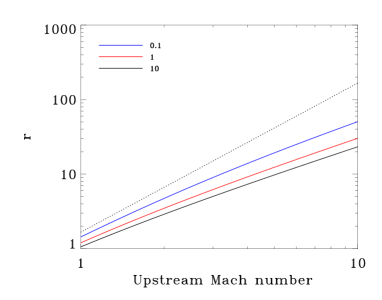
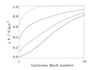
Figure 3: Evolution of the compression ratio, $r$, and of the amount of kinetic energy radiated away, $X$, as a function of the upstream Mach number for a barotropic material, with density ratio $r_{1}=0.1$ (black), $1$ (red), and $10$ (blue). The dotted lines represents the evolution for a supercritical shock with a optically thin upstream material (c.f. Fig. 2).

Figure 3 illustrates the evolution of the adimensional quantities $r$ and $X$ as a function of the upstream Mach number for a barotropic material, for density ratio $r_{1}=0.1$, $1$, and $10$, which represent transition values between the optically thin (isothermal) and thick regimes (adiabatic). For comparison, we also plot again the evolution of $r$ and $X$ for a supercritical shock with an optically thin upstream material. The compression ratio is not bound by a limiting value as the upstream Mach number increases, as for the case of a supercritical shock with an optically thin upstream material, but in contrast to the case of an opaque material. The compression ratio decreases as $r_{1}$ increases (note that for $r_{1}=10$, the material should be totally optically thick in the context of star formation). The shock is never found to be supercritical ($X\sim 1$), even though almost all the incident kinetic energy is assumed to be radiated away at high upstream Mach number. This clearly shows that a barotropic EOS approximation cannot treat properly radiative shocks. Compared to the case of a supercritical shock with an optically thin upstream which is relevant for the accretion shock on the first Larson core in the transition regions between the isothermal and adiabatic regime, the compression ratio and the amount of energy radiated away are underestimated.

The specific entropy jump at the shock is expressed as

$$\Delta s=s_{2}-s_{1}=C_{\mathrm{v}}\left[\ln\left(\frac{P_{2}}{\rho_{2}^{\gamma}}\right)-\ln\left(\frac{P_{1}}{\rho_{1}^{\gamma}}\right)\right],$$ (32)

where $s$ is the specific entropy and $C_{\mathrm{v}}=k_{\mathrm{B}}/(\mu m_{\mathrm{H}}(\gamma-1))$. The entropy jump for a barotropic fluid is thus proportional to $\Pi/r^{\gamma}$. Figure 4 shows the evolution of log$(\Pi/r^{\gamma})$ for a barotropic fluid (with $r_{1}=0.1$, 1, and 10) and for a shock with an optically thin upstream material. The entropy jump at the shock is overestimated with a barotropic law. This would lead to an incorrect initial entropy level and profile for new born protostars. The entropy is indeed a key quantity for pre-main sequence evolutionary models as it entirely determines the mass-radius relationship of an adiabatic object, like the Larson cores.

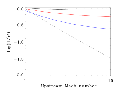
Figure 4: Evolution of the entropy jump, $\Delta s\propto\Pi/r^{\gamma}$, as a function of the the upstream Mach number for a barotropic material, with density ratio $r_{1}=0.1$ (black), $1$ (red), and $10$ (blue). The dotted line represents the evolution for a supercritical shock with an optically thin upstream material.

In this section, we have shown that the downstream quantities of radiative shocks strongly depend on the nature of the shock and on the model used to describe radiation transport. In the following sections, we study in detail the case of a particular radiative shock: the accretion shock on the first Larson core, in the context of star formation.

3 1D spherical numerical calculations - Method.

3.1 Introduction and previous work

In this subsection, we introduce our numerical method and basics concepts, for a good understanding of the following part of this work.

The two companion papers Masunaga et al. (1998), and Masunaga & Inutsuka (2000) present a very extensive study of 1D protostellar collapse. The first paper focusses on the formation and the properties of the first core, using a frequency dependent RHD model, while the second paper addresses the formation of the second core These authors use a 1D spherical code in the Lagrangean frame. Moment equations of radiation in the comoving frame are solved following Stone et al. (1992). Masunaga et al. (1998) use a variable Eddington tensor factor (VETF) that retains a frequency dependence, whereas grey opacities are used to calculate the coupling between matter and radiation and the work of the radiative pressure.

In Masunaga et al. (1998), the cores initially have uniform density and temperature, and a radius adjusted so that the cloud should be initially slightly more massive than the Jeans mass. Initial masses range from $0.1$ M_⊙ to $3$ M_⊙. They find that whatever the initial cloud mass, the first core radius $R_{\mathrm{fc}}$ is almost constant, with $R_{\mathrm{fc}}\sim 5$ AU, and the first core mass is $M_{\mathrm{fc}}\sim 0.05$ M_⊙. In their study, $R_{\mathrm{fc}}$ is defined as the point where the gas pressure is balanced by the ram pressure of the infalling envelope.

To compare our numerical results with analytical theories, it is useful to define some measurable quantities. A useful one is the mass accretion rate $\dot{M}$. For a 1D spherical model, the mass accretion rate is simply $\dot{M}=4\pi r^{2}\rho u$. In the theory, the accretion rate is generally defined as (e.g. Stahler et al., 1980)

$$\dot{M}=\xi\frac{c^{3}_{s0}}{G},$$ (33)

where $\xi$ is a dimensionless coefficient and $c_{s0}$ the isothermal sound speed. $\xi$ is estimated assuming that a non-magnetic, non-rotating cloud, whose initial state corresponds approximately to a balance between thermal support and self-gravity, has comparable free-fall time, $t_{\mathrm{ff}}\sim R_{c}^{3/2}/(GM_{c})^{1/2}$, and sound-crossing time, $t_{\mathrm{sc}}\sim R_{c}/c_{s0}$. The mass accretion rate is thus given by $\dot{M}\sim M_{c}/t_{\mathrm{ff}}$. Shu (1977) obtained $\xi=0.975$ for the expansion-wave solution, whereas the dynamic Larson-Penston solution yields $\xi\sim 50$ (Larson, 1969; Penston, 1969).

Another quantity directly comparable to the theory is the accretion luminosity, usually expressed as

$$L^{\mathrm{acc}}_{\mathrm{fc}}=\frac{GM_{\mathrm{fc}}\dot{M}}{R_{\mathrm{fc}}},$$ (34)

where $M_{\mathrm{fc}}$ corresponds to the mass of the accreting core. This accretion luminosity thus corresponds to the case where all the infalling kinetic energy is radiated away, i.e. to a supercritical radiative shock. The accretion luminosity can be directly measured in numerical calculations, from the mass accretion rate, and compared with the intrinsic effective luminosity emerging from the first core.

3.2 Numerical method

We use a 1D full Lagrangean version of the code developed by Chièze and Audit (see Audit et al., 2002), that integrates the equations of grey radiation hydrodynamics under three different assumptions (in order of increasing complexity order): a barotropic EOS, the flux limited diffusion approximation (FLD) and the M1 model. The RHD equations are integrated in their non-conservative forms using finite volumes and an artificial viscosity scheme in tensorial form. The RHD equations are integrated with an implicit scheme in time, using a standard Raphson-Newton iterative method.

3.3 General assumptions for the radiation field

The first approximation in our calculations is to consider a grey radiation field, i.e. only one group of photons, integrated over all frequencies. We also neglect scattering and assume Local Thermodynamical Equilibrium (LTE) everywhere. The second assumption concerns the coupling between radiation and hydrodynamics, for which we write the RHD equations in the comoving frame.

3.4 Models for the radiative transfer

According to previous studies using accurate model for the radiation field (e.g. Masunaga et al., 1998), it is well established that the molecular gas follows two thermal regimes during the first collapse. At low density, the gas is able to radiate freely and to couple with the dust. This is the isothermal regime, where the Jeans mass decreases with density. Then, when the gas becomes denser, typically $\rho>\rho_{\mathrm{ad}}\sim 1\times 10^{-13}$ g cm^-3, the radiation is trapped within the gas that begins to heat up adiabatically. The Jeans mass then increases with density until the gas becomes hot enough to dissociate H₂, leading to the onset of the second collapse.

3.4.1 The barotropic equation of state approximation

As mentioned earlier, the easiest way to describe the thermal evolution of the gas without solving the radiative transfer equation is to adopt a barotropic EOS that reproduces both the isothermal and adiabatic limiting regimes as a function of the density. We use the following barotropic EOS:

$$\frac{P}{\rho}=c_{\mathrm{s}}^{2}=c_{s0}^{2}\left[1+\left(\frac{\rho}{\rho_{\mathrm{ad}}}\right)^{2/3}\right],$$ (35)

where $\rho_{\mathrm{ad}}$ is the critical density at which the gas becomes adiabatic. This critical density is obtained by more accurate calculations and depends on the opacities, the composition and the geometry of the molecular gas. At low densities, $\rho\ll\rho_{\mathrm{ad}}$, $c_{\mathrm{s}}\sim c_{s0}=0.19$ km s^-1 (for $T\sim 10$ K), the molecular gas is able to radiate freely by thermally coupling to the dust and remains isothermal at 10 K. At high densities, $\rho>\rho_{\mathrm{ad}}$, we assume that the cooling due to radiative transfer is trapped by the dust opacity. Therefore, $P\propto\rho^{5/3}$, which corresponds to an adiabatic, monoatomic gas with adiabatic exponent $\gamma=5/3$. Molecular hydrogen behaves like a monoatomic gas until the temperature reaches several hundred Kelvin since the rotational degrees of freedom are not excited at lower temperatures (Whitworth & Clarke, 1997; Masunaga & Inutsuka, 2000).

3.4.2 Moment Models

In RHD calculations, the radiative transfer equation should be formally integrated over 6 dimensions at each time step. This process is too computationally demanding for multidimensional numerical analysis. Using angular moments of the transfer equation is thus very useful, by allowing a large reduction of the computational cost. However, each evolution equation of a moment of the transfer equation involves the next higher order moment of the intensity. Consequently, as for the kinetic theory of gases, the system must be closed by using an ad hoc relation that gives the highest moment as a function of the lower order moments. For radiation transport, the closure theory is usually limited to the two first moments of the transfer equation. A closure relation for the system is needed and this relation is of prime importance. Many possible choices for the closure relation exist. In the following, we present two models based on more or less accurate closure relations, that we use in this work: the flux limited diffusion (FLD) approximation and the M1 model.

3.4.3 The Flux Limited Diffusion approximation

The diffusion approximation is the most widely used moment model of radiation transport. The diffusion limit is valid when the photon mean free path is small compared with other length scales in the system. On the contrary, the approximation is no longer accurate in the transport regime. In the diffusion limit, photons diffuse through the material in a random walk. Readers can find an accurate derivation of the diffusion limit in Mihalas & Mihalas (1984), §80.

In the diffusion limit, the radiative energy $E_{\mathrm{r}}$ and radiative flux $\textbf{F}_{\mathrm{r}}$ are simply related by

$$\textbf{F}_{\mathrm{r}}=-\frac{c}{3\kappa_{\mathrm{R}}}\nabla E_{\mathrm{r}},$$ (36)

where $\kappa_{\mathrm{R}}$ is the Rosseland mean opacity. The radiative flux is expressed directly as a function of the radiative energy and is proportional and collinear to the radiative energy gradient. Equation (36) has no upper limit, but for optically thin flows, the effective propagation speed of the radiation must be limited to $c$ ($\textbf{F}_{\mathrm{r}}\leq cE_{\mathrm{r}}$). We thus have to limit the propagation speed of the radiation by means of a flux limiter. Equation (36) is then expressed as

$$\textbf{F}_{\mathrm{r}}=-\frac{c\lambda}{\kappa_{\mathrm{R}}}\nabla E_{\mathrm{r}},$$ (37)

where $\lambda=\lambda(R)$ is the flux limiter.

In this study, we retain the flux limiter derived by Minerbo (1978)

$$\lambda=\left\{\begin{array}[]{ccc}2/(3+\sqrt{9+12R^{2}})&\mathrm{if}&0\leq R\leq 3/2,\\ (1+R+\sqrt{1+2R})^{-1}&\mathrm{if}&3/2<R\leq\infty,\end{array}\right.$$ (38)

with $R=|\nabla E_{\mathrm{r}}|/(\kappa_{\mathrm{R}}E_{\mathrm{r}})$. The flux limiter has the property that $\lambda\rightarrow 1/3$ in optically thick regions and $\lambda\rightarrow 1/R$ in optically thin regions.

In the FLD approximation, an unique diffusion-type equation on the radiative energy is thus obtained

$$\frac{\partial E_{\mathrm{r}}}{\partial t}-\nabla\cdot\left(\frac{c\lambda}{\kappa_{\mathrm{R}}}\nabla E_{\mathrm{r}}\right)=\kappa_{\mathrm{P}}(4\pi B-cE_{\mathrm{r}}).$$ (39)

3.4.4 M1 model

In the M1 model, the radiation transport is described by the first two moments of the radiative transfer equation (radiative energy and flux). We use a closure relation introduced by Dubroca & Feugeas (1999). The M1 method is used in the RHD code HERACLES (González et al., 2007). Based on a minimum entropy principle, this method is able to account for large anisotropy of the radiation as well as for the correct diffusion limit. The main advantage of the M1 system is that the underlying photon distribution function is not isotropic, but has a preferential direction of propagation. The M1 model also allows to explicitly get rid of the ad-hoc limitation of the flux in the transport regime.

Let us consider the evolution equations of the zeroth and first moments of the specific intensity in the laboratory frame

$$\left\{\begin{array}[]{llll}\partial_{t}E_{\mathrm{r}}+\nabla\cdot\textbf{F}_{\mathrm{r}}&=&\kappa_{\mathrm{P}}(4\pi B-cE_{\mathrm{r}})\\ \partial_{t}\textbf{F}_{\mathrm{r}}+c^{2}\nabla\cdot\mathbb{P}_{\mathrm{r}}&=&-\kappa_{\mathrm{R}}c\textbf{F}_{\mathrm{r}}\end{array}\right.,$$ (40)

where $\kappa_{\mathrm{P}}$ is the Planck mean opacity. Note that we use the Rosseland mean in the first moment equation in order to yield the diffusion limit. As a closure relation, the radiative pressure is often expressed as $\mathbb{P}_{\mathrm{r}}=\mathbb{D}E_{\mathrm{r}}$, where $\mathbb{D}$ is the Eddington tensor. Assuming that the direction of the radiative flux is an axis of symmetry of the local specific intensity, the Eddington tensor is given by (Levermore, 1984)

$$\mathbb{D}=\frac{1-\chi}{2}\mathbb{I}+\frac{3\chi-1}{2}\textbf{n}\otimes\textbf{n},$$ (41)

where $\chi$ is the Eddington factor, $\mathbb{I}$ the identity matrix and $\textbf{n}=\frac{\textbf{f}}{f}$ a unit vector aligned with the radiative flux. In the M1 approximation, the Eddington factor $\chi$ is then obtained by minimizing the radiative entropy (Dubroca & Feugeas, 1999). The Eddington factor is then found to be

$$\chi=\frac{3+4f^{2}}{5+2\sqrt{4-3f^{2}}}.$$ (42)

It is then trivial to recover the two asymptotic regimes of radiative transfer. When $f\rightarrow 0$, $\chi=1/3$ and $\mathbb{P}_{\mathrm{r}}=1/3E_{\mathrm{r}}\mathbb{I}$ which corresponds to the diffusion limit with an isotropic radiative pressure. On the other hand, if $f=1$, $\chi=1$ and $\mathbb{P}_{\mathrm{r}}=\textbf{n}\otimes\textbf{n}E_{\mathrm{r}}$, which corresponds to the free-streaming limit. Between these two limits, the closure relation ensures that energy remains positive and that the flux is limited ($\textbf{F}_{\mathrm{r}}<cE_{\mathrm{r}}$).

3.4.5 Systems of RHD equations

• In the barotropic EOS approximation, the thermal behavior of the gas is determined by the choice of the EOS. The energy equation becomes superfluous and the Euler equations reduce to :

  $$\left\{\begin{array}[]{llll}\partial_{t}\rho+\nabla\left[\rho\textbf{u}\right]&=&0\\ \partial_{t}\rho\textbf{u}+\nabla\left[\rho\textbf{u}\otimes\textbf{u}+P\mathbb{I}\right]&=&-\rho\nabla\Phi,\\ \end{array}\right.$$ (43)

  where $\Phi$ the gravitational potential.
  

• In the FLD approximation, the system of RHD equations corresponds to the Euler equations plus the equation on the radiative energy

  $$\left\{\begin{array}[]{ccccl}\partial_{t}\rho&+&\nabla\left[\rho\textbf{u}\right]&=&0\\ \partial_{t}\rho\textbf{u}&+&\nabla\left[\rho\textbf{u}\otimes\textbf{u}+P\mathbb{I}\right]&=&-\rho\nabla\Phi+\lambda\nabla E_{\mathrm{r}}\\ \partial_{t}E&+&\nabla\left[\textbf{u}\left(E+P\right)\right]&=&-\rho\textbf{u}\cdot\nabla\Phi+\lambda\nabla E_{\mathrm{r}}\cdot\textbf{u}\\ &&&&-\kappa_{\mathrm{P}}(4\pi B-cE_{\mathrm{r}})\\ \partial_{t}E_{\mathrm{r}}&+&\nabla\left[\textbf{u}E_{\mathrm{r}}\right]&=&-\mathbb{P}_{\mathrm{r}}:\nabla\textbf{u}+\nabla\cdot\left(\frac{c\lambda}{\kappa_{\mathrm{R}}}\nabla E_{\mathrm{r}}\right)\\ &&&&+\kappa_{\mathrm{P}}(4\pi B-cE_{\mathrm{r}}).\end{array}\right.$$ (44)

  This system is closed by the perfect gas relation and the simplest FLD approximation for the radiative pressure, $\mathbb{P}_{\mathrm{r}}=\lambda E_{\mathrm{r}}$.
  

• In the M1 model, we consider the equations governing the evolution of an inviscid, radiating fluid

  $$\left\{\begin{array}[]{ccccl}\partial_{t}\rho&+&\nabla\left[\rho\textbf{u}\right]&=&0\\ \partial_{t}\rho\textbf{u}&+&\nabla\left[\rho\textbf{u}\otimes\textbf{u}+P\mathbb{I}\right]&=&-\rho\nabla\Phi+\kappa_{\mathrm{R}}\textbf{F}_{\mathrm{r}}/c\\ \partial_{t}E&+&\nabla\left[\textbf{u}\left(E+P\right)\right]&=&-\rho\textbf{u}\cdot\nabla\Phi+\kappa_{\mathrm{R}}\textbf{F}_{\mathrm{r}}/c\cdot\textbf{u}\\ &&&&-\kappa_{\mathrm{P}}(4\pi B-cE_{\mathrm{r}})\\ \partial_{t}E_{\mathrm{r}}&+&\nabla\left[\textbf{u}E_{\mathrm{r}}\right]+\nabla\cdot\textbf{F}_{\mathrm{r}}&=&-\mathbb{P}_{\mathrm{r}}:\nabla\textbf{u}+\kappa_{\mathrm{P}}(4\pi B-cE_{\mathrm{r}})\\ \partial_{t}\textbf{F}_{\mathrm{r}}&+&\nabla\left[\textbf{u}\textbf{F}_{\mathrm{r}}\right]+c^{2}\nabla\cdot\mathbb{P}_{\mathrm{r}}&=&-\left(\textbf{F}_{\mathrm{r}}\cdot\nabla\right)\textbf{u}-\kappa_{\mathrm{R}}c\textbf{F}_{\mathrm{r}}.\end{array}\right.$$ (45)

  where $\rho$ is the material density, u is the velocity, $P$ the isotropic thermal pressure, $\Phi$ the gravitational potential and $E$ the fluid total energy $E=\rho\epsilon+1/2\rho u^{2}$. This system is closed by the perfect gas relation and the M1 relation (42).

3.5 Initial and boundary conditions

We use the same model as Masunaga et al. (1998), i.e. a uniform density sphere of mass $M_{0}=1$ M_⊙, temperature $T_{0}=10$ K ($c_{s0}=0.187$ km s^-1) and radius $R_{0}=10^{4}$ AU. This initial setup corresponds to a ratio $\alpha$ of thermal to gravitational energies of $\alpha=5R_{0}k_{\mathrm{B}}T_{0}/(2GM_{0}\mu m_{\mathrm{H}})\sim 0.97$ and to a free-fall time t${}_{\mathrm{ff}}\sim 1.77\times 10^{5}$ yr. Boundary conditions are very simple: for hydrodynamics, we impose a constant thermal pressure equal to the initial pressure (other quantities are free) and for the radiation field, we impose a vanishing gradient on radiative temperature. Calculations have been performed using a Lagrangean grid containing 4500 cells.

3.6 The opacities

For the M1 model and the FLD approximation, we use the set of opacities given by Semenov et al. (2003) for low temperature ($<1000$ K) and Ferguson et al. (2005) for high temperature ($>1000$ K), that we compute as a function of the gas temperature and density. In Fig. 5, the table for the Rosseland opacity is plotted as a function of temperature and density. In Semenov et al. (2003), the dependence of the evaporation temperatures of ice, silicates and iron on gas density are taken into account. In this work, we use spherical composite aggregate particles for the grain structure and topology and a normal iron content in the silicates, Fe/(Fe + Mg)=0.3.

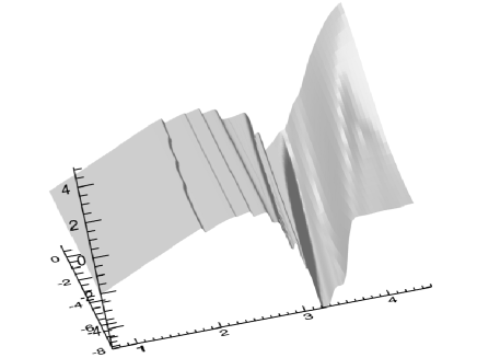
Figure 5: Rosseland opacity made of a mix of Semenov et al. (2003) model at low temperature and Ferguson et al. (2005) model at high temperature. The Rosseland mean opacity is plotted as a function of temperature ($x$-axis) and $R=\rho/(T^{3}_{6})$, with $T_{6}=T/10^{6}$, ($y$-axis) using logarithm scales.

4 1D numerical calculations of the first collapse

As we mentioned before, all calculations presented here have been performed with 4500 cells, distributed according to a logarithmic scale in mass in our initial setup. These mass and spatial resolutions are sufficient to resolve quantitatively the accretion shock energy budget (see appendix A).

Calculations with the barotropic EOS have been performed using a critical density of $\rho_{\mathrm{ad}}=3.7\times 10^{-13}$ g cm^-3 . We derived the value of $\rho_{\mathrm{ad}}$ from the intersection of extrapolated lines of the isotherm and the adiabat in the log($\rho$)-log($T$) plane, obtained with calculations using the M1 model (see Fig. 6).

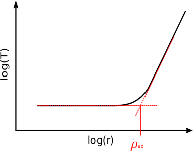
Figure 6: Sketch of the estimate of $\rho_{\mathrm{ad}}$ used in the barotropic EOS, according to the density-temperature distribution obtained with the M1 model.

4.1 Results during the first collapse. Formation of the first core.

Table 1 gives results of barotropic EOS (Baro), M1, and FLD calculations, when the central density reaches $\rho_{c}=1\times 10^{-10}$ g cm^-3. Note that for all calculations, the dynamical times are very close to $\sim 0.189$ Myr $\sim 1.07$ t_ff. We define the first core radius as the radius at which the infall velocity is the largest (i.e., the position of the accretion shock). The accretion luminosity is estimated at the first core border, according to equation (34). The mass accretion rate $\dot{M}$ and the accretion parameter $\xi$ are evaluated at $R_{\mathrm{fc}}$. Table 1 also displays the central temperature $T_{\mathrm{c}}$, the central specific entropy $s_{\mathrm{c}}$, and the first core temperature at the border $T_{\mathrm{fc}}$.

As seen from table 1, the first core radius and mass agree well with Masunaga et al. (1998) results. The results from the M1 or FLD calculations are very similar. The central temperature with the FLD is slightly higher (by $\sim 2\%$) than the one in the M1 calculations, which confirms the fact that the diffusion approximation tends to slightly overestimate the cooling. The central entropy obtained with the M1 and FLD models is lower than the one obtained with the barotropic EOS, and this difference increases with time. Indeed, taking into account radiative transfer allows the energy to be radiated away during the collapse, a process which is not properly handled with a barotropic EOS. This leads to a lower entropy level of the first core with the FLD or the M1 models. The temperature at the border of the first core is higher in the M1 and FLD cases, since the photons escaping the accretion shock heat up the infalling material. On the other hand, the mass accretion rate, the mass, the radius and the accretion parameter $\xi$ of the first core are in good agreement between the three models. Note that the values of $\xi$ obtained in our calculations are closer to the Larson-Penston solution than to Shu’s expansion wave solution.

Model	$R_{\mathrm{fc}}$	$M_{\mathrm{fc}}$	$\dot{M}$	$L_{\mathrm{acc}}$	$T_{\mathrm{c}}$	$T_{\mathrm{fc}}$	$s_{\mathrm{c}}$	$\xi$
	(AU)	(M⊙)	(M${}_{\odot}/$yr)	(L⊙)	(K)	(K)	(erg K-1 g-1)
Baro	6.8	$2.35\times 10^{-2}$	$4.2\times 10^{-5}$	0.021	551	15	$2.03\times 10^{9}$	27
FLD	8.1	$2.33\times 10^{-2}$	$4.1\times 10^{-5}$	0.019	411	58	$2.02\times 10^{9}$	26
M1	7.8	$2.33\times 10^{-2}$	$4.1\times 10^{-5}$	0.018	419	57	$2.02\times 10^{9}$	26

Table 1: Summary of first core properties for $\rho_{c}=1\times 10^{-10}$ g cm^-3.

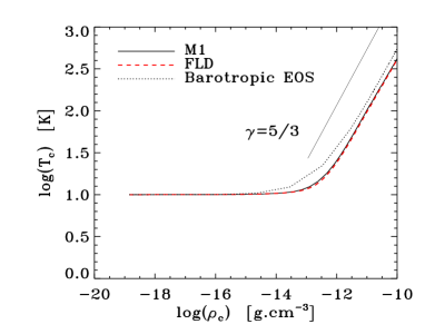
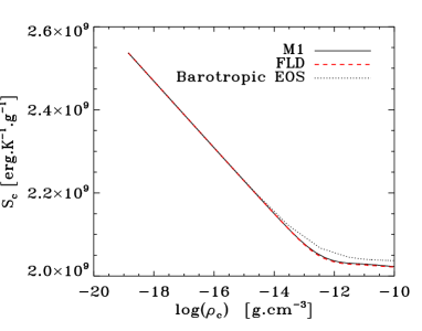
Figure 7: Evolution of the central temperature ( left) and the central entropy (right) as a function of the central density during the first collapse for the M1 (solid line), FLD (dashed red line) and barotropic (dashed-dotted line).

Figure 7 shows the evolution of the central temperature and the central entropy as a function of the central density. From Fig. 7(a), we notice the perfect bimodal thermal behavior of the gas, from isothermal to adiabatic. The critical density at which the gas begins to heat in both M1 and FLD calculations is the same. The difference with the barotropic case stems from our choice of the barotropic EOS and critical density. For FLD and M1, we find a slope of $\gamma_{\mathrm{eff}}-1\sim 0.61<2/3$ at high density. This means that the first core is not completely adiabatic, but experiences some heat loss, yielding a significant cooling.

In Fig. 7(b), the central entropy is plotted as a function of the central density. At high density, we recover the adiabatic regime, and the M1 and FLD calculations settle at the same entropy level in the center, that is lower than the one reached by the barotropic model. In the barotropic case, the entropy is determined by the EOS. The value of the “adiabat” at which the gas settles is

$$s\propto\ln\left(\frac{P}{\rho^{\gamma}}\right).$$ (46)

For the barotropic EOS, we have

$$s\propto\ln\left[\rho^{-2/3}c_{s0}^{2}\left(1+\left(\frac{\rho}{\rho_{\mathrm{ad}}}\right)^{2/3}\right)\right]\propto\ln\left(\frac{c_{s0}^{2}}{\rho_{\mathrm{ad}}^{2/3}}+\frac{c_{s0}^{2}}{\rho^{2/3}}\right).$$ (47)

At high density, $s\rightarrow\ln(c_{s0}^{2}/\rho_{\mathrm{ad}}^{2/3})$. The limiting value for the entropy is then $\sim 2.03\times 10^{9}$ erg K^-1 g^-1 for the barotropic EOS, which is higher than the value obtained with FLD and M1. Moreover, as the slope of the thermal profile (fig. 7(a)) is not exactly equal to $\gamma=5/3$ in the M1 and FLD calculations, as mentioned above, the gas tends to cool and to decrease its entropy level at a rate $\sim 10^{-3}$-$10^{-4}$ erg K^-1 g^-1 s^-1 at the center. This is one of the immediate and most important consequences of correctly taking into account radiative transfer in the collapse: the accretion shock becomes a real radiative shock and radiation is transported outward in the core.

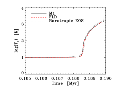
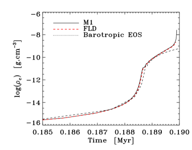
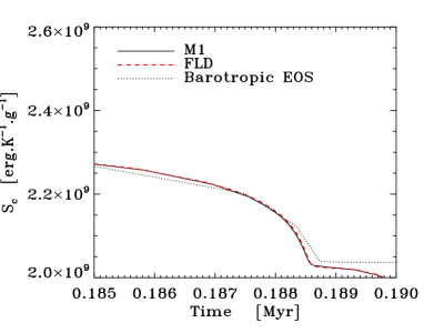
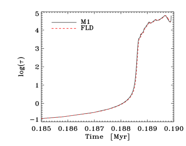
Figure 8: Evolution of the central temperature, density, entropy and optical depth with time for the M1 (solid line), FLD (dashed red line) and barotropic (dashed-dotted line) models.

Figure 8 shows the central temperature, density, entropy and optical depth evolution during the collapse. Variations of all variables are quite similar for temperature lower than T$\sim 100$ K. At 100 K, there is a first discontinuity in the opacity, due to the destruction of icy grains. This discontinuity moves to higher temperature as density increases, so that density affects to some extent the opacity. However, these differences are really small. From Fig. 8(c), we clearly see that the entropy level remains constant with the barotropic model, whereas the first core keeps cooling to lower entropy levels with the M1 and FLD calculations. This is an important result, since, as mentioned previously, the entropy level of a low mass protostar determines its mass-radius relationship, and thus its pre-main sequence subsequent evolution. According to the first principle of thermodynamics, the global entropy loss of the first core can be estimated as

$$\left(\frac{\partial L}{\partial m}\right)_{t}=-T\left(\frac{\partial s}{\partial t}\right)_{m}=-\left(\frac{\partial\epsilon}{\partial t}\right)_{m}-P\left(\frac{\partial v}{\partial t}\right)_{m},$$ (48)

where $\epsilon$ is the specific internal energy and $v=1/\rho$ is the specific volume. If the first core was perfectly adiabatic, the compressional work would be entirely converted into internal energy, and the radiative loss would be zero. As shown in Fig 9f, the luminosity increases significantly within the first core in the FLD and M1 calculations. This increase corresponds to the radiative loss, which amounts to $\sim 4\times 10^{-3}$ L_⊙. The corresponding entropy loss of the first core is then

$$\frac{\Delta s_{\mathrm{fc}}}{\Delta t}\sim-\frac{1}{T}\frac{\Delta L}{M_{\mathrm{fc}}}.$$ (49)

At $\rho_{c}=1\times 10^{-10}$ g cm^-3, we get $M_{\mathrm{fc}}\sim 2.3\times 10^{-2}$ M_⊙. The entropy loss is thus

$$\frac{\Delta s_{\mathrm{fc}}}{\Delta t}\sim-\frac{3.3\times 10^{-1}}{T}\hskip 6.0pt\mathrm{erg}\hskip 3.0pt\mathrm{K}^{-1}\mathrm{g}^{-1}.$$ (50)

For a typical first core temperature of a few 100 K, the entropy loss rate is $\sim 10^{-3}$ erg K^-1 g^-1 yr^-1, which is consistent with the value found at the center. The first core lasting about a few hundred years, the total entropy loss thus represents a few percents of the core’s initial entropy content, and this entropy loss increases with time, as shown in Fig. 1 of Masunaga et al. (1998). Such an entropy loss cannot be handled with a barotropic EOS.

In Fig. 8(d), we see that the first core quickly becomes optically thick once it begins to heat up. The optical depth at the center is so high that observations are not able to catch the central evolution of the cores at this stage of the evolution.

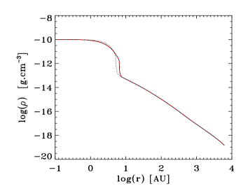
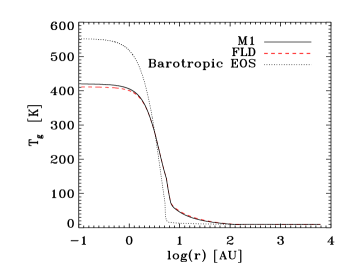
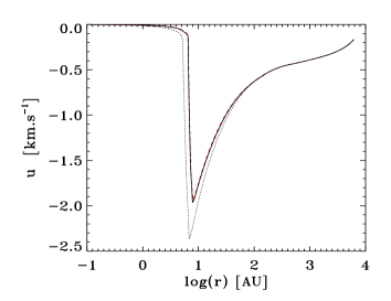
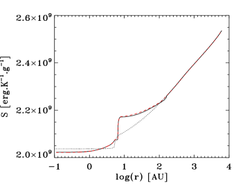
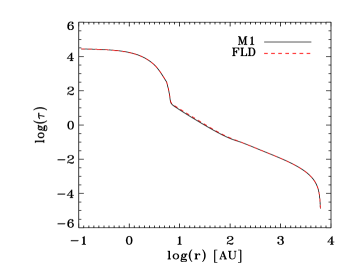
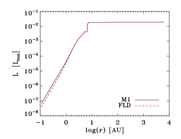
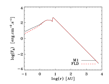
Figure 9: Radial profiles of various properties during the collapse of a 1 M_⊙ dense clump for a core central density $\rho_{c}=1\times 10^{-10}$ g cm^-3, for the M1 (solid line), FLD (dashed red line) and barotropic (dashed-dotted line) models. From top left to bottom right: (a) density, (b) gas temperature, (c) velocity, (d) entropy, (e) optical depth, (f) luminosity, (g) radiative flux and (h) integrated mass.

4.2 Mechanical and thermal profile of the first prestellar core.

Figure 9 displays the radial profiles of the density, gas temperature, velocity, specific entropy, optical depth, luminosity, radiative flux and integrated mass, once the central density reaches $\rho_{c}=1\times 10^{-10}$ g cm^-3, for calculations with M1, FLD and the barotropic EOS. As mentioned before, the first core radius is smaller with the barotropic model, whereas both M1 and FLD results are similar. For the latter models, we find only small differences around $\tau\sim 1$, i.e. at the transition between the optically thick and thin regimes. Since the M1 model naturally recovers the diffusion and transport regimes and since the FLD model is defined as to recover these limits as well, it is natural that we get similar results when either the transport or the diffusion regimes are well established. Although the accretion shock is located within the transition region around $\tau\sim 10$, the aforementioned small differences do not affect the first core properties. The entropy jump at the accretion shock is much higher with M1 and FLD than with the barotropic approximation. We also see from the temperature and entropy profiles that the barotropic EOS cannot handle correctly the transition from the isothermal to the adiabatic regime, as pointed out earlier. The radiative precursor in front of the shock is not reproduced with the barotropic EOS. In that case, the gas becomes rapidly isothermal after the shock, whereas it is heated by photons escaping from the shock in the FLD and M1 models. As a consequence, the core temperature is higher in the barotropic case. The differences in the behavior of the radiative flux at small radius come from the differences in temperature between the M1 and FLD models.

The emergent luminosity, on the other hand, is the same for both the M1 and FLD models. The luminosity jump, $\sim 0.013$ L_⊙ is consistent with the accretion luminosity estimated from equation (34), $0.014$ L_⊙. This means that all the infalling kinetic energy is radiated away at the shock boundary, i.e. that the shock is supercritical at the formation of the first core.

If we apply the criterion derived in equations (20) and (21) to the upstream quantities estimated in Fig. 9, i.e. $\rho_{1}\sim 7\times 10^{-14}$ g cm^-3, $u_{1}\sim 2\times 10^{5}$cm s^-1, and $T_{1}\sim 57$ K, the corresponding critical temperatures are $T_{\mathrm{cr}}\sim 23$ K with (20) and $T_{\mathrm{cr}}\sim 57$ K with (21). This confirms the fact that the accretion shock on the first core is supercritical. However, since accretion takes place in the transition region between optically thin and thick regimes and since most of the upstream region is optically thin (see luminosity and optical depth profiles in Fig. 9), the most relevant model is the one we developed for a supercritical shock with a upstream optically thin material.

4.3 Comparison with an analytical model

In Sect. 2, we have developed a semi-analytical solver that can be applied to the accretion radiative shock on the first core and that covers three cases: the case of sub- or super-critical shocks in an optically thick material and the case of a supercritical shock in an optically thin material. In the following, we develop a simple model for the protostellar collapse, where the upstream quantities are estimated under some basic assumptions, and we compare this model with our numerical results. We need to estimate the density, the velocity and the temperature in the preshock region in the context of the first core formation. We can easily get the density (and the velocity) from the Larson-Penston and Shu self-similar solutions. The tricky part is to estimate the temperature before the shock. However, as mentioned in §2.4, the preshock temperature is determined by the upstream velocity. Assuming that the accretion shock is supercritical and that the upstream material is optically thin, it is then easy to get this temperature and to recover all fluid variables. Omukai (2007) proposes an alternative model that fully describes the first core characteristics but does not use jump relations for a radiating fluid. In our model, we consider the characteristics at the first core border and the jump conditions for a radiating fluid.

We approximate the upstream velocity by the free-fall velocity

$$u_{\mathrm{1,ff}}=\sqrt{\frac{2GM_{\mathrm{fc}}}{R_{\mathrm{fc}}}}.$$ (51)

The preshock density is given assuming a profile $\propto r^{-2}$ in the free-falling envelope

$$\rho_{1}=\frac{c_{s}^{2}}{2\pi G}R_{\mathrm{fc}}^{-2},$$ (52)

where $c_{s}=(P/\rho)^{1/2}$ is the isothermal sound speed (at 10 K). The temperature is estimated by assuming a supercritical shock, i.e. all the upstream kinetic energy being radiated away. Moreover, our calculations using the FLD or M1 models yield $\mathcal{M}_{1}\sim 2$ and Fig. 2 shows that $X\sim 1$. The shock temperature thus reads (c.f. equation 22)

$$\sigma T_{\mathrm{s}}^{4}=\frac{\rho_{1}u_{1,\mathrm{ff}}^{3}}{2}.$$ (53)

We take the first core properties obtained in our numerical calculations, similar to those in Masunaga et al. (1998), i.e. $M_{\mathrm{fc}}\sim 2.3\times 10^{-2}$ M_⊙ and $R_{\mathrm{fc}}\sim 8$ AU. If we apply equations (51), (52) and (53) to these quantities, we get: $\rho_{1}=5.8\times 10^{-14}$ g cm^-3, $u_{1}\sim 2.3\times 10^{5}$ cm s^-1 and $T_{1}\sim 50$ K.

We now apply these preschock quantities to the jump properties derived in Sect. 2.2.2 for a supercritical shock with an optically thin upstream material. According to eq. 14, we get $r=\rho_{2}/\rho_{1}\sim 50$, which gives $\rho_{2}\sim 2.9\times 10^{-12}$ g cm^-3, and $u_{2}=4.6\times 10^{3}$ cm s^-1. Using equation (15), we get $X\sim 0.99$: all the infalling kinetic energy is radiated away at the shock.

We can compare these analytical results with the numerical ones, given in Fig. 9 and in Table 1: $\rho_{1}\sim 7\times 10^{-14}$ g cm^-3, $u_{1}\sim 2\times 10^{5}$ cm s^-1 and $T_{1}=57$ K. Thus, the analytical estimates for the preshock quantities agree quite well with the numerical values. We also read from the figure and table $\rho_{2}\sim 2.15\times 10^{-12}$ g cm^-3, $u_{2}\sim 10^{4}$ cm s${}^{-1}\ll u_{1}$, again very similar to our analytical estimates. These comparisons validate our simple analytical model to infer the properties of the first Larson’s core.

5 Summary and perspectives

In this paper, we have conducted RHD calculations aimed at describing the physical and radiative properties of radiative shocks. We have applied these calculations to the formation of the first Larson’s core, during the early phases of protostellar collapse. We have also derived simple analytical models and compared the results with the ones obtained in the simulations. The main results of our study can be summarized as follows :

1. The properties of the first collapse and the characteristics of the first core in our calculations are in good agreement with the ones obtained by Masunaga et al. (1998). We find that the first core has a typical radius of $\sim 8$ AU and a mass $\sim 2\times 10^{-2}$ M_⊙. This sets up the initial conditions for the second collapse and the formation of the second Larson’s core.

2. We show that, at the first core stage, the accretion shock is a supercritical radiative shock, at which all the infalling kinetic energy is radiated away, and that a barotropic EOS cannot reproduce the correct jump conditions at the shock. The FLD and M1 calculations show that there is a substantial entropy loss during the formation of the first core, due to the radiative loss. A barotropic EOS cannot handle correctly this cooling mechanism. In consequence, the first core’s entropy content obtained with a barotropic approximation is overestimated, compared with the calculations which solve the radiative transfer. Such a cooling effect can have a strong impact on the core fragmentation process and, eventually on the initial properties of the future protostar (Commerçon et al., in prep).

3. We confirm that, when radiative cooling is properly taken into account, the transition from an isothermal to an adiabatic phase during the first collapse and the formation of the first Larson’s core does not necessarily correspond to an optical depth of unity, as shown initially by Masunaga & Inutsuka (1999).

4. We develop a simple analytical model for supercritical shocks within an optically thin medium, which reproduces well the jump conditions obtained with the numerical calculations. We show that the compression ratio in such a kind of shock can become very high ($r\sim 50$). We plan in the future to keep exploring this issue with a frequency dependent radiative transfer model. Indeed, strong shocks on (massive) protostars are known to be optically thick for hard photons, while optically thin for UV radiation (e.g. Stahler et al., 1980).

5. We show that, at least in 1D spherical calculations, the flux limited diffusion approximation is appropriate to study the earliest stages of star formation, as it gives very similar results as the more complete M1 model for radiative transfer. Note, however, that our 1D spherical geometry code cannot account for multi dimensional effects like the anisotropy of the radiation field.

This study confirms the necessity to solve the complete RHD equations, i.e. to correctly take into account the coupling between radiation and hydrodynamics, when addressing strong shock conditions, as occurring during the formation of the first Larson’s core in the context of star formation. Such a complete, consistent treatment of radiation and hydrodynamics is necessary to correctly handle the cooling properties of the accreting gas and thus to obtain the correct mechanical and thermal properties of the first core. This, in turn, sets up the initial conditions for the second collapse and the formation of the second core. Indeed, since the first core has a short lifetime (a few hundred years), it is important to pursue these calculations during the second collapse, including H₂ dissociation. Such work is under progress.

Appendix A Effect of the numerical resolution on the energy budget through the shock. Case of a $0.01$ M_⊙ dense core.

In contrast to the hydrodynamical case, the structure of a radiative shock can extend over large distances, depending on the optical properties of the material. For an optically thin material, the photon mean free path is large, so the shock structure is very extended compared to the viscous scale. In this work (see Sect. 3), we present numerical calculations of dense core collapse, using a fix resolution in mass, i.e. the mesh is not refined in the large gradient zones. Although this Lagrangean description is well suited for the hydrodynamical shocks, thanks to the artificial viscosity scheme, it may encounter difficulties in the case of radiation-hydrodynamical flows, in particular in the optically thin region (upstream region, outside the first core).

In this appendix, we present the results of the collapse of a 0.01 M_⊙ dense core, using the same initial ratio of thermal energy over gravitational energy as in Sec 3 ($\alpha\sim 0.97$). To investigate the effect of the numerical resolution, we performed calculations with 4500 cells and 18000 cells, using the FLD model.

Figure 10 shows the density, gas temperature, velocity, entropy, optical depth and luminosity radial profiles for the 2 calculations at a central density $\rho_{c}\sim 1.6\times 10^{-11}$ g cm^-3. Although there are some significative differences in the radiative precursor region (i.e. the transition region between optically thin and thick regions, where $2<\tau<0.5$) and in the estimate of the first core radius ($\sim 10\%$), the entropy, density, velocity and luminosity jumps are about the same. In both calculations, the shock is supercritical and the amount of energy radiated away is about the same ($L=1.5\times 10^{-2}$ with 4500 cells, and $L=1.44\times 10^{-2}$ with 18000 cells). This means that the overall properties of the first accretion shock, including its global energy budget remain correctly calculated even at low resolution. However, using 18000 cells, we see that the spike in the gas temperature is resolved and that the radiative precursor length is much smaller. On the other hand, the central entropy within the first core is the same in both cases, indicating that the cooling of the first core by radiation is not affected by the lack of resolution in the radiative shock.

Figure 11 shows the normalized energy balance at $\rho_{c}=1.8\times 10^{-11}$ g cm^-3 for the calculations run with 18000 cells (left) and 4500 cells (right). The figures display the rate of change of potential energy $dE_{\mathrm{p}}/dt$, kinetic energy $dE_{\mathrm{k}}/dt$, internal energy $dU_{\mathrm{i}}/dt$, total energy $d(E_{\mathrm{k}}+E_{\mathrm{p}}+U_{\mathrm{i}})/dt$, and the work done by thermal pressure and radiative flux ($L_{\mathrm{rad}}+4\pi r^{2}Pu$). The total energy equation reads:

$$\frac{d}{dt}\left(U_{\mathrm{i}}+E_{\mathrm{k}}+E_{\mathrm{p}}+E_{\mathrm{r}}\right)+\frac{\partial}{\partial r}\left[4\pi r^{2}[u(p+P_{\mathrm{r}})+F_{\mathrm{r}}]\right]=0.$$ (54)

First, we see form fig. 11 that the radiative pressure exerts a negligible work compared to the thermal pressure. Comparing the energy balance of the two calculations, we see that it is globally the same, which confirms that the calculations done with 4500 cells get the correct features of the first core accretion shock, even though the radiative structure of this shock is not resolved.

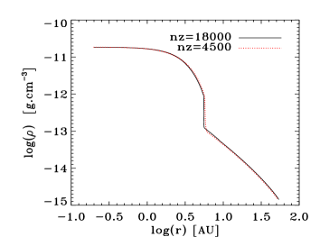
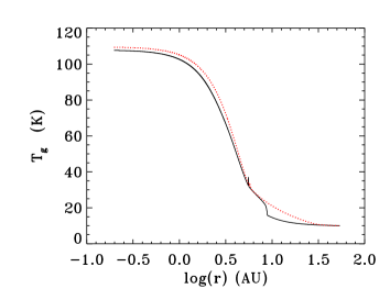
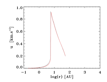
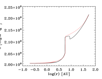
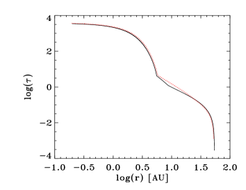
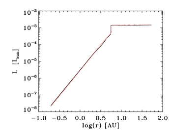
Figure 10: Radial profiles of various 1st core properties during the collapse of a 0.01 M_⊙ clump for a core central density $\rho_{c}=1.8\times 10^{-11}$ g cm^-3, for calculations done with 4500 cells (dotted red line) and 18 000 cells (solid black line). From top left to bottom right: (a) density, (b) gas temperature, (c) entropy, (d) velocity, (e) optical depth, (f) luminosity.

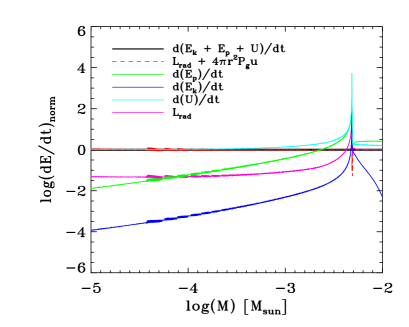
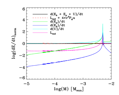
Figure 11: Normalized energy balance as a function of the mass for the calculations done with 18000 cells (left) and 4500 cells (right), when the central density reaches $\rho_{c}=1.8\times 10^{-11}$ g cm^-3. Scales are logarithmic and normalized to the rate of change of the total energy $d(E_{\mathrm{k}}+E_{\mathrm{p}}+U_{\mathrm{i}})/dt$.

.