A FEniCS-Based Programming Framework for Modeling Turbulent Flow by the Reynolds-Averaged Navier-Stokes Equations

Abstract

Finding an appropriate turbulence model for a given flow case usually calls for extensive experimentation with both models and numerical solution methods. This work presents the design and implementation of a flexible, programmable software framework for assisting with numerical experiments in computational turbulence. The framework targets Reynolds-averaged Navier-Stokes models, discretized by finite element methods. The novel implementation makes use of Python and the FEniCS package, the combination of which leads to compact and reusable code, where model- and solver-specific code resemble closely the mathematical formulation of equations and algorithms. The presented ideas and programming techniques are also applicable to other fields that involve systems of nonlinear partial differential equations. We demonstrate the framework in two applications and investigate the impact of various linearizations on the convergence properties of nonlinear solvers for a Reynolds-averaged Navier-Stokes model.

1 Introduction

Turbulence is the rule rather than the exception when water flows in nature, but finding the proper turbulence model for a given flow case is demanding. There exists a large number of different turbulence models, and a researcher in computational turbulence would benefit from being able to easily switch between models, combine models, refine models and implement new ones. As the models consist of complex, highly nonlinear systems of partial differential equations (PDEs), coupled with the Navier-Stokes (NS) equations, constructing efficient and robust iteration techniques is model- and problem-dependent, and hence subject to extensive experimentation. Flexible software tools can greatly assist the researcher experimenting with models and numerical methods. This work demonstrates how flexible software can be designed and implemented using modern programming tools and techniques.

Precise prediction of turbulent flows is still a very challenging task. It is commonly accepted that solutions of the Navier-Stokes equations, with sufficient resolution of all scales in space and time (Direct Numerical Simulation, DNS), describe turbulent flow. Such an approach is, nevertheless, computationally feasible only for low Reynolds number flow and simple geometries, at least for the foreseeable future. Large Eddy Simulations (LES), which resolve large scale motions and use subgrid models to represent the unresolved scales are computationally less expensive than DNS, but are still too expensive for the simulation of turbulent flows in many practical applications. A computationally efficient approach to turbulent flows is to work with Reynolds-averaged Navier-Stokes (RANS) models. RANS models involve solving the incompressible NS equations in combination with a set of transport equations for statistical turbulence quantities. The uncertainty in RANS models lies in the extra transport equations, and for a given flow problem it is a challenge to pick an appropriate model. There is hence a need for a researcher to experiment with different models to arrive at firm conclusions on the physics of a problem.

Most commercial computational fluid dynamics (CFD) packages contain a limited number of turbulence models, but allow users to add new models through “user subroutines” which are called at each time level in a simulation. The implementation of such routines can be difficult, and new models might not fit easily within the constraints imposed by the design of the package and the “user subroutine” interface. The result is that a specific package may only support a fraction of the models that a practitioner would wish to have access to. There is a need for CFD software with a flexible design so that new PDEs can be added quickly and reliably, and so that solution approaches can easily be composed. We believe that the most effective way of realizing such features is to have a programmable framework, where the models and numerics are defined in terms of a compact, high-level computer language with a syntax that is based on mathematical language and abstractions.

A software system for RANS modeling must provide higher-order spatial discretizations, fine-grained control of linearizations, support for both Picard and Newton type iteration methods, under-relaxation, restart of models, combinations of models and the easy implementation of new PDEs. Standard building blocks needed in PDE software, such as forming coefficient matrices and solving linear systems, can act as black boxes for a researcher in computational turbulence. To the authors’ knowledge, there is little software with the aforementioned flexibility for incompressible CFD. There are, however, many programmable environments for solving PDEs. A non-exhaustive list includes Cactus ⁷, COMSOL Multiphysics ¹¹, deal.II ^{12 2}, Diffpack ¹³, DUNE ¹⁶, FEniCS ¹⁹³⁷, Dular and Geuzaine ¹⁵, GetFEM++ ²⁰, OpenFOAM ⁴³, Overture ⁴⁴, Proteus ⁴⁷ and SAMRAI ⁵¹. Only a few of these packages have been extensively used for turbulent flow. OpenFOAM ⁴³ is a well-structured and widely used object-oriented C++ framework for CFD, based on finite volume methods, where new models can quite easily be added through high-level C++ statements. Overture ⁴⁴,⁶ is also an object-oriented C++ library used for CFD problems, allowing complex movements of overlapping grids. Proteus ⁴⁷ is a modern Python- and finite element-based software environment for solving PDEs, and has been used extensively for CFD problems, including free surface flow and RANS modeling. FEniCS ¹⁹, ³⁶ is a recent C++/Python framework, where systems of PDEs and corresponding discretization and iteration strategies can be defined in terms of a few high-level Python statements which inherit the mathematical structure of the problem, and from which low level code is generated. The approach advocated in this work utilizes FEniCS tools. All FEniCS components are freely available under GNU general public licenses ¹⁹. A number of application libraries that make use of the FEniCS software have been published ⁵⁷. For instance, cbc.solve ⁹ is a framework for solving the incompressible Navier-Stokes equations and the Rheology Application Engine (Rheagen) ⁴⁸ is a framework for simulating non-Newtonian flows. Both applications share some of the features of the current work.

Traditional simulation software packages are usually implemented in Fortran, C, or C++ because of the need for high computational performance. A consequence is that these packages are less user-friendly and flexible, but far more efficient, than similar projects implemented in scripting languages such as Matlab or Python. In FEniCS, scripting is combined with symbolic mathematics and code generation to provide both user-friendliness and efficiency. Specifically, the Unified Form Language (UFL), a domain-specific language for the specification of variational formulations of PDEs, is embedded within the programming language Python. Variational formulations are then just-in-time compiled into C++ code for efficiency. The generated C++ code can be expected to outperform hand-written quadrature code since special-purpose PDE compilers ¹, ²⁸, ⁴² are employed. UFL has built-in support for automatic differentiation, derivation of adjoint equations, etc., which makes it particularly useful for complicated and coupled PDE problems.

Several authors have addressed how object-oriented and generative programming can be used to create flexible libraries for solving PDEs, but there are significantly fewer contributions dealing with the design of frameworks on top of such libraries for addressing multi-physics problems and coupling of PDEs ⁴⁵, ³¹, ³³, ²³, ⁵⁴, ⁴⁰, ⁵⁰. These contributions focus on how the C++ or Fortran 90 languages can be utilized to solve such classes of problems. This work builds on these cited works, but applies Python as programming language and FEniCS as tool for solving PDEs. Python has strong support for dynamic classes and object orientation, and since variables are not declared in Python, generative programming comes without any extra syntax (in contrast with templates in C++). Presented code examples from the framework will demonstrate how these features, in combination with FEniCS, result in clean and compact code, where the specification of PDE models and linearization strategies can be expressed in a mathematical syntax.

FEniCS supports finite element schemes, including discontinuous Galerkin methods ⁴¹, but not finite difference methods. Many finite volume methods can be constructed as low-order discontinuous Galerkin methods using FEniCS ⁵⁵. Despite the development of several successful methods for solving the NS equations and LES models by finite element methods, finite element methods have not often been applied to RANS models, though some research contributions exist in this area ²¹, ³, ⁵², ³⁸.

The remainder of this paper is organized as follows. Section 2 demonstrates the use of FEniCS for solving simple PDEs and briefly elaborates some key aspects of FEniCS. Section 3 presents a selection of PDEs which form the basis of some common RANS models. Finite element formulations of a typical RANS model and the iteration strategies for handling nonlinear equations appear in Section 4. The software framework for NS solvers and RANS models is described in Section 5. Section 6 demonstrates two applications of the framework and investigates the impact of different types of linearizations. In Section 7 we briefly discuss the computational efficiency of the framework, and some concluding perspectives are drawn in Section 8. The code framework we describe, cbc.rans, is open source and available under the Lesser GNU Public license ⁸.

2 FEniCS for solving differential equations

FEniCS is a collection of software tools for the automated solution of differential equations by finite element methods. FEniCS includes tools for working with computational meshes, linear algebra and finite element variational formulations of PDEs. In addition, FEniCS provides a collection of ready-made solvers for a variety of partial differential equations.

2.1 Solving a partial differential equation

To illustrate how PDEs can be solved in FEniCS, we consider the weighted Poisson equation $-\nabla\cdot(\kappa\nabla u)=f$ in some domain $\Omega\subset\mathbb{R}^{d}$ with $\kappa=\kappa(x)$ a given coefficient. On a subset of the boundary, denoted by $\partial\Omega_{D}$, we prescribe a Dirichlet condition $u=0$, while on the remainder of the boundary, denoted by $\partial\Omega_{R}$, we prescribe a Robin condition $-\kappa{\partial u/\partial n}=\alpha(u-u_{0})$, where $\alpha$ and $u_{0}$ are given constants.

To solve the above boundary-value problem, we first need to define the corresponding variational problem. It reads: find $u\in V$ such that

$$F\equiv\int_{\Omega}\kappa\nabla u\cdot\nabla v\,dx-\int_{\Omega}fv\,dx+\int_{\partial\Omega_{R}}\alpha(u-u_{0})v\,ds=0\quad\forall\,v\in V,$$ (1)

where $V$ is the standard Sobolev space $H^{1}(\Omega)$ with $u=v=0$ on $\partial\Omega_{D}$. The function $u$ is known as a trial function and $v$ is known as a test function. We can partition $F$ into a “left-hand side” $a(u,v)$ and a “right-hand side” $L(v)$,

$$F=a(u,v)-L(v),$$ (2)

where

$$a(u,v) =\int_{\Omega}\kappa\nabla u\cdot\nabla v\,dx+\int_{\partial\Omega_{R}}\alpha uv\,ds,$$ (3)

$$L(v) =\int_{\Omega}fv\,dx+\int_{\partial\Omega_{R}}\alpha u_{0}v\,ds.$$ (4)

For numerical approximations, we work with a finite-dimensional subspace $V_{h}\subset V$ and aim to find an approximation $u\in V_{h}$ such that

$$a(u,v)=L(v)\quad\forall\ v\in V_{h}.$$ (5)

This leads to a linear system $AU=b$, where $A_{ij}=a(\phi_{j},\phi_{i})$ and $b_{i}=L(\phi_{i})$ are the matrix and vector obtained by evaluating the bilinear form $a$ the and linear $L$ for the basis functions of the discrete finite element function space and $U\in\mathbb{R}^{N}$ is the vector of expansion coefficients for the finite element solution $u(x)=\sum_{j=1}^{N}U_{j}\phi_{j}(x)$.

To solve equation (5) in FEniCS, all we have to do is (i) define a mesh of triangles or tetrahedra over $\Omega$; (ii) define the boundary segments $\partial\Omega_{D}$ and $\partial\Omega_{R}$ (only $\partial\Omega_{D}$ has to be defined in this case); (iii) define the function space $V_{h}$; (iv) define $F$; (v) extract the left-hand side $a$ and the right-hand side $L$; (vi) assemble the matrix $A$ and the vector $b$ from $a$ and $L$, respectively; and (vii) solve the linear system $AU=b$. To be specific, we take $d=2$, $x=(x_{0},x_{1})$, $\kappa(x_{0},x_{1})=x_{1}\sin(\pi x_{0})$, $f(x_{0},x_{1})=0$, $g(x_{0},x_{1})=0$, and $\alpha=10$ and $u_{0}=2$. The following Python program performs the above steps (i)–(vii):

from dolfin import *mesh = Mesh(’mydomain.xml.gz’)dOmega_D = MeshFunction(’uint’, mesh, ’myboundary.xml.gz’)V = FunctionSpace(mesh, ’Lagrange’, degree=1)g = Constant(0.0)bc = DirichletBC(V, g, dOmega_D)u = TrialFunction(V)v = TestFunction(V)f = Constant(0.0)k = Expression(’x[1]*sin(pi*x[0])’)alpha = 10; u0 = 2F = inner(k*grad(u), grad(v))*dx - f*v*dx + alpha*(u-u0)*v*dsa = lhs(F); A = assemble(a)L = rhs(F); b = assemble(L)bc.apply(A, b) # set Dirichlet conditionssolve(A, u.vector(), b, ’gmres’, ’ilu’)plot(u)The FEniCS tools used in this program are imported from the dolfin package, which defines classes like Mesh, DirichletBC, FunctionSpace, TrialFunction, TestFunction, and key functions such as assemble, solve and plot. We first load a mesh and boundary indicators from files. Alternatively, the mesh and boundary indicators can be defined as part of the program. The type of discrete function space is defined in terms of a mesh, a class of finite element (here ’Lagrange’ means standard continuous Lagrange finite elements ⁵) and a polynomial degree. The function space V used in the program corresponds to continuous piecewise linear elements on triangles. In addition to continuous piecewise polynomial function spaces, FEniCS supports a wide range of finite element methods, including arbitrary order continuous and discontinuous Lagrange elements, and arbitrary order $H(\rm div)$ and $H(\rm curl)$ elements. The full range of supported elements is listed in Logg and Wells ³⁷.

The variational problem is expressed in terms of the Unified Form Language (UFL), which is another component of FEniCS. The key strength of UFL is the close correspondence between the mathematical notation for $F$ and its Python implementation F. Constants and expressions can be compactly defined and used as parts of variational forms. Terms multiplied by dx correspond to volume integrals, while multiplication by ds implies a boundary integral. Meshes may include several subdomains and boundary segments, each with its corresponding volume or boundary integral. From the variational problem F, we may use the operators lhs and rhs to extract the left- and right-hand sides which may then be assembled into a matrix A and a vector b by calls to the assemble function. The Dirichlet boundary conditions may then be enforced as part of the linear system $AU=b$ by the call bc.apply(A, b). Finally, we solve the linear system using the generalized minimal residual method (’gmres’) with ILU preconditioning (’ilu’).

2.2 Solving a system of partial differential equations

The Stokes problem is now considered. It will provide a basis for the incompressible Navier-Stokes equations in the following section. The Stokes problem, allowing for spatially varying viscosity, involves the system of equations

$$-\nabla\cdot\nu(\nabla{\mbox{\boldmath$u$}}+\nabla{\mbox{\boldmath$u$}}^{T})+\nabla p ={\mbox{\boldmath$f$}},$$ (6)

$$\nabla\cdot{\mbox{\boldmath$u$}} =0.$$ (7)

For the variational formulation, we introduce a vector test function ${\mbox{\boldmath$v$}}\in{\mbox{\boldmath$V$}}$ for (6) and a scalar test function $q\in Q$ for (7). The trial functions are ${\mbox{\boldmath$u$}}\in{\mbox{\boldmath$V$}}$ and $p\in Q$. Typically, ${\mbox{\boldmath$V$}}=[V]^{d}$, where $V$ is the space defined for the Poisson problem, and $Q$ can be taken as the standard space $L^{2}(\Omega)$. The corresponding variational formulation reads: find $({\mbox{\boldmath$u$}},p)\in{\mbox{\boldmath$V$}}\times Q$ such that

$$F\equiv\int_{\Omega}\nu(\nabla{\mbox{\boldmath$u$}}+\nabla{\mbox{\boldmath$u$}}^{T}):\nabla{\mbox{\boldmath$v$}}\,dx-\int_{\Omega}p\nabla\cdot{\mbox{\boldmath$v$}}\,dx-\int_{\Omega}\nabla\cdot{\mbox{\boldmath$u$}}\,q\,dx\\ -\int_{\Omega}{\mbox{\boldmath$f$}}\cdot{\mbox{\boldmath$v$}}\,dx=0\quad\forall\ ({\mbox{\boldmath$v$}},q)\in V\times Q.$$ (8)

For simplicity, we consider in this example only problems where boundary integrals vanish. As with the Poisson equation, we obtain a linear system for the degrees of freedom of the discrete finite element solutions by using finite-dimensional subspaces of $V$ and $Q$. Note the negative sign in front of the third term in $F$. The sign of this term is arbitrary, but it has been made negative such that the resulting matrix will be symmetric, which is a feature that can be exploited by some preconditioners and iterative solvers.

The following code snippet demonstrates the essential steps for solving the Stokes problem in FEniCS:

V = VectorFunctionSpace(mesh, ’Lagrange’, degree=2)Q = FunctionSpace(mesh, ’Lagrange’, degree=1)VQ = V * Q # Taylor-Hood mixed finite elementu, p = TrialFunctions(VQ)v, q = TestFunctions(VQ)U = Function(VQ)f = Constant((0.0, 0.0)); nu = Constant(1e-6)F = nu*inner(grad(u) + grad(u).T, grad(v))*dx - p*div(v)*dx \     - div(u)*q*dx - inner(f, v)*dxA, b = assemble_system(lhs(F), rhs(F), bcs)solve(A, U.vector(), b, ’gmres’, ’amg_hypre’)u, p = U.split()We have for brevity omitted the code for loading a mesh, defining boundaries and specifying Dirichlet conditions (the boundary conditions are assumed to be available as a list bcs in the program). A mixed Taylor-Hood element is simply defined as V*Q, where V is a second-order vector Lagrange element and Q is a first-order scalar Lagrange element. Note that we solve for U, which is a mixed finite element function containing $u$ and $p$. The function U can be split into individual finite element functions, u and p, corresponding to $u$ and $p$.

More detailed information on the usage of and possibilities with the FEniCS software suite can be found in the literature ²⁶, ²⁷, ³⁵, ³⁶, ²⁵, ³⁷, ⁴⁹.

2.3 Automatic code generation

At the core of FEniCS is the C++/Python library DOLFIN ³⁷, which provides data structures for finite element meshes, functionality for I/O, a common interface to linear algebra packages, finite element assembly, handling of parameters, etc. DOLFIN differs from other finite element libraries in that it relies on generated code for some core tasks. In particular, DOLFIN relies on generated code for the assembly of finite element variational forms. Code can be generated from a form expressed in UFL by one of the two form compilers FFC ²⁶ and SFC ¹ that are available as part of FEniCS. The code may be generated prior to compile-time by explicitly calling one of the form compilers, or automatically at run-time (just-in-time compilation). The latter is the default behavior for users of the FEniCS Python interface.

Relying on generated code means that FEniCS is able to satisfy two seemingly contradictory objectives: generality, by being capable of generating code for a large class of linear and nonlinear finite element variational problems, and efficiency by calling highly optimized code generated for each specific variational problem given by the user as input. This is illustrated in Figure 1. It has been demonstrated ²⁹, ²⁵, ²⁶, ²⁷, ²⁸, ⁴² that using form compilers permits the application of optimizations and representations that could not be expected in handwritten code.

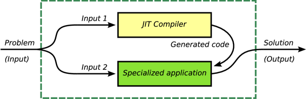
Figure 1: Sketch of the code generation process in FEniCS. The user input is partitioned into two sets: data that requires special-purpose code such as finite element variational forms (Input 1), and data that can be handled efficiently by a general purpose routine such as the mesh, boundary conditions and coefficients (Input 2). For the first set of data, FEniCS calls a just-in-time (JIT) compiler to generate special-purpose code that may then be executed for the remaining set of data (Input 2) to compute the solution.

3 Reynolds averaged Navier-Stokes equations

Turbulent flows are described by the NS equations. On a domain $\Omega\subset\mathbb{R}^{d}$ for time $t\in(0,t_{s}]$, the incompressible NS equations read

$$\frac{\partial{\mbox{\boldmath$U$}}}{\partial t}+{\mbox{\boldmath$U$}}\cdot\nabla{\mbox{\boldmath$U$}} =-\frac{1}{\varrho}\nabla P+\nabla\cdot\nu(\nabla{\mbox{\boldmath$U$}}+\nabla{\mbox{\boldmath$U$}}^{T})+{\mbox{\boldmath$f$}},$$ (9)

$$\nabla\cdot{\mbox{\boldmath$U$}} =0,$$ (10)

where ${\mbox{\boldmath$U$}}({\mbox{\boldmath$x$}},t)$ is the velocity, $P({\mbox{\boldmath$x$}},t)$ is the pressure, $\nu$ is the kinematic viscosity, $\varrho$ is the mass density and $f$ represents body forces. The incompressible NS equations must be complemented by initial and appropriate boundary conditions to complete the problem.

Simulations of turbulent flows are usually computationally expensive because of the need for extreme resolution in both space and time. However, in most applications the average quantities are of interest. In the statistical modeling of turbulent flows, the velocity and pressure are viewed as random space-time fields which can be decomposed into mean and fluctuating parts: ${\mbox{\boldmath$U$}}={\mbox{\boldmath$u$}}+{\mbox{\boldmath$u$}}^{\prime}$ and $P=p+p^{\prime}$, where $u$ and $p$ are ensemble averages of $U$ and $P$, respectively, and ${\mbox{\boldmath$u$}}^{\prime}$ and $p^{\prime}$ are the random fluctuations about the mean field. Inserting these decompositions into (9) and (10) results in a system of equations for the mean quantities $u$ and $p$:

$$\frac{\partial{\mbox{\boldmath$u$}}}{\partial t}+{\mbox{\boldmath$u$}}\cdot\nabla{\mbox{\boldmath$u$}} =-\frac{1}{\varrho}\nabla p+\nabla\cdot\nu(\nabla{\mbox{\boldmath$u$}}+\nabla{\mbox{\boldmath$u$}}^{T})-\nabla\cdot\overline{{\mbox{\boldmath$u$}}^{\prime}\otimes{\mbox{\boldmath$u$}}^{\prime}}+{\mbox{\boldmath$f$}},$$ (11)

$$\nabla\cdot{\mbox{\boldmath$u$}} =0,$$ (12)

where ${\mbox{\boldmath$R$}}=\overline{{\mbox{\boldmath$u$}}^{\prime}\otimes{\mbox{\boldmath$u$}}^{\prime}}$, known as the Reynolds stress tensor, is the ensemble average of ${\mbox{\boldmath$u$}}^{\prime}\otimes{\mbox{\boldmath$u$}}^{\prime}$. The Reynolds stress tensor is unknown and solving equations (11) and (12) requires approximating $R$ in terms of $u$, $\nabla{\mbox{\boldmath$u$}}$, or other computable quantities.

A general observation on turbulence is that it is dissipative. This observation has led to the idea of relating the Reynolds stress to the strain rate tensor of the mean velocity field, ${\mbox{\boldmath$S$}}=(\nabla{\mbox{\boldmath$u$}}+\nabla{\mbox{\boldmath$u$}}^{T})/2$. More specifically,

$${\mbox{\boldmath$R$}}=-2\nu_{T}{\mbox{\boldmath$S$}}+{\frac{2}{3}}k{\mbox{\boldmath$I$}},$$ (13)

where $\nu_{T}$ is the “turbulent viscosity”, $k=\overline{{\mbox{\boldmath$u$}}^{\prime}\cdot{\mbox{\boldmath$u$}}^{\prime}}/2$ is the turbulent kinetic energy and $I$ is the identity tensor. Many models have been proposed for the turbulent viscosity. The most commonly employed “one-equation” turbulence model is that described by Spalart and Allmaras ⁵³. It involves a transport equation for a “viscosity” parameter, coupled to 11 derived quantities with 9 model parameters.

Two-equation turbulence models represent the largest class of RANS models, providing two transport equations for the turbulence length and time scales. This family of models includes the $k$–$\epsilon$ models ²², ³⁴ and the $k$–$\omega$ models ⁵⁶. Of the two-equation models, we limit our considerations in this work to $k$–$\epsilon$ models. Due to severe mesh resolution requirements these models usually involve the use of wall functions instead of regular boundary conditions on solid walls. Support for the use of wall functions has been implemented in the current framework and special near-wall modifications are employed both for the standard $k$–$\epsilon$ model and the more elaborate four equation $v^{2}$–$f$ model ¹⁸. Implementation aspects of these wall modifications, though, involves a level of detail that is beyond the scope of the current presentation. For this reason we will mainly focus on a particular family of $k$–$\epsilon$ models, the low-Reynolds models, that apply standard Dirichlet boundary conditions on solid walls.

The “pseudo” rate of dissipation of turbulent kinetic energy is defined as⁴⁶

$$\epsilon=\nu\overline{\nabla{\mbox{\boldmath$u$}}^{\prime}:\nabla{\mbox{\boldmath$u$}}^{\prime}}.$$ (14)

All $k$–$\epsilon$ models express the turbulent viscosity parameter $\nu_{T}$ in terms of $k$ and $\epsilon$ (from dimensional arguments, $\nu_{T}\sim k^{2}/\epsilon$). The fluctuations ${\mbox{\boldmath$u$}}^{\prime}$ are unknown, and consequently $k$ and $\epsilon$ must be modeled. A low-Reynolds $k$–$\epsilon$ model in general form reads

$$\frac{\partial{\mbox{\boldmath$u$}}}{\partial t}+{\mbox{\boldmath$u$}}\cdot\nabla{\mbox{\boldmath$u$}} =\nabla\cdot\nu_{u}(\nabla{\mbox{\boldmath$u$}}+\nabla{\mbox{\boldmath$u$}}^{T})-\frac{1}{\varrho}\nabla p+{\mbox{\boldmath$f$}},$$ (15)

$$\nabla\cdot{\mbox{\boldmath$u$}} =0,$$ (16)

$${\frac{\partial k}{\partial t}}+{\mbox{\boldmath$u$}}\cdot\nabla k =\nabla\cdot(\nu_{k}\nabla k)+P_{k}-\epsilon-D,$$ (17)

$${\frac{\partial\epsilon}{\partial t}}+{\mbox{\boldmath$u$}}\cdot\nabla\epsilon =\nabla\cdot(\nu_{\epsilon}\nabla\epsilon)+\left(C_{\epsilon 1}P_{k}-C_{\epsilon 2}f_{2}\epsilon\right)\frac{\epsilon}{k}+E,$$ (18)

$$\nu_{u} =\nu+\nu_{T},$$ (19)

$$\nu_{k} =\nu+\frac{\nu_{T}}{\sigma_{k}},$$ (20)

$$\nu_{\epsilon} =\nu+\frac{\nu_{T}}{\sigma_{\epsilon}},$$ (21)

$$\nu_{T} =C_{\mu}f_{\mu}{\frac{k^{2}}{\epsilon}},$$ (22)

$$P_{k} ={\mbox{\boldmath$R$}}:\nabla{\mbox{\boldmath$u$}},$$ (23)

where various terms which are model-specific are defined in Table 1 for three common low-Reynolds models. The pressure $p$ in the NS equations is a modified pressure that includes the kinetic energy from the model for the Reynolds stresses. The dissipation rate term $\epsilon$ is also modified and the pseudo-dissipation rate defined in (14) can be recovered from these models as $\epsilon+D$. This modification is introduced in all low-Reynolds models to allow a homogeneous Dirichelt boundary condition for $\epsilon$ on solid walls. Further discussion of boundary conditions for RANS models are delayed until the presentation of examples in Section 6.

	Chien 10	Launder and Sharma 34	Jones and Launder 22
$C_{\mu}$	0.09	0.09	0.09
$\sigma_{k}$	1	1	1
$\sigma_{\epsilon}$	1.3	1.3	1.3
$D$	$2\nu\frac{k}{y^{2}}$	$2\nu|\nabla\sqrt{k}|^{2}$	$2\nu|\nabla\sqrt{k}|^{2}$
$E$	$-\frac{2\nu\epsilon}{y^{2}}\exp\left(-0.5y^{+}\right)$	$2\nu\nu_{T}|\nabla^{2}{\mbox{\boldmath$u$}}|^{2}$	$2\nu\nu_{T}|\nabla^{2}{\mbox{\boldmath$u$}}|^{2}$
$C_{\epsilon 1}$	1.35	1.44	1.55
$C_{\epsilon 2}$	1.8	1.92	2.0
$f_{\mu}$	$1-\exp(-0.0115y^{+})$	$\exp\left(\frac{-3.4}{(1+Re_{T}/50)^{2}}\right)$	$\exp\left(\frac{-2.5}{(1+Re_{T}/50)}\right)$
$f_{2}$	$1-0.22\exp\left(-\frac{Re_{T}^{2}}{36}\right)$	$1-0.3\exp\left(-{Re}_{T}^{2}\right)$	$1-0.3\exp\left(-{Re}_{T}^{2}\right)$

Table 1: Various model constants and damping functions for three low-Reynolds number turbulence models. $Re_{T}=k^{2}/(\nu\epsilon)$.

In the original models of Jones and Launder ²² and Launder and Sharma ³⁴ $D=2\nu({\partial\sqrt{k}}/{\partial y})^{2}$ and $E=2\nu\nu_{T}({\partial^{2}u_{x}}/{\partial y^{2}})$, where $y$ is the wall normal direction and $u_{x}$ is the mean velocity tangential to the wall. To eliminate the coordinate dependency, we have generalized these terms to the ones seen in Table 1. The rationale behind the generalization is that $D$ and $E$ are only important in the vicinity of walls, where the term $\partial u_{x}/\partial y$ will be dominant. The generalized terms will therefore approach the terms in the original model in the regions where the terms are significant, regardless of the geometry of the wall.

4 Numerical methods for the Reynolds averaged Navier-Stokes equations and models

This section addresses numerical solution methods for the Navier-Stokes equation presented in (15) and (16) and the turbulence models presented in Section 3. RANS models are normally considered in a stationary setting, i.e., the mean flow quantities do not depend on time. Hence, we will here ignore the time derivatives appearing in the equations in Section 3, even though we have also implemented solvers for transient systems within the current framework. We also adopt the strategy of splitting the total system of PDEs into (i) the Navier-Stokes system for $u$ and $p$, with $R$ given; and (ii) a system of equations for $R$, with $u$ and $p$ given.

4.1 Navier-Stokes solvers

There are numerous approaches to solving the NS equations. A common choice is a projection or pressure correction scheme ³², ¹⁴. Here we present a solver in which $u$ and $p$ are solved in a coupled fashion. The variational form consists of that for the Stokes problem in Section 2.2, with an additional momentum convection term. With $\varrho$ absorbed into $p$, the variational problem for the NS equations reads: find $({\mbox{\boldmath$u$}},p)\in{\mbox{\boldmath$V$}}\times Q$ such that

$$F\equiv\int_{\Omega}({\mbox{\boldmath$u$}}\cdot\nabla{\mbox{\boldmath$u$}})\cdot{\mbox{\boldmath$v$}}\,dx+\int_{\Omega}\nu_{u}(\nabla{\mbox{\boldmath$u$}}+\nabla{\mbox{\boldmath$u$}}^{T}):\nabla{\mbox{\boldmath$v$}}\,dx-\int_{\Omega}p\nabla\cdot{\mbox{\boldmath$v$}}\,dx\\ -\int_{\Omega}(\nabla\cdot{\mbox{\boldmath$u$}})q\,dx-\int_{\Omega}{\mbox{\boldmath$f$}}\cdot{\mbox{\boldmath$v$}}\,dx=0\quad\forall\ ({\mbox{\boldmath$v$}},q)\in{\mbox{\boldmath$V$}}\times Q.$$ (24)

For low “cell” Reynolds numbers, equation (24) is stable provided appropriate finite element bases are used for $u$ and $p$. For example, the Taylor-Hood element, with continuous second-order Lagrange functions for the velocity and continuous first-order Lagrange functions for the pressure is stable. It may sometimes be advantageous to use equal-order basis functions for the velocity and pressure field, in which case a stabilizing term must be added to the equations to control spurious pressure oscillations. Consider the residual of the Navier-Stokes momentum equation (15):

$$\mathcal{R}\equiv{\mbox{\boldmath$u$}}\cdot\nabla{\mbox{\boldmath$u$}}+\nabla p-\nabla\cdot\nu_{u}(\nabla{\mbox{\boldmath$u$}}+\nabla{\mbox{\boldmath$u$}}^{T})-{\mbox{\boldmath$f$}}.$$ (25)

We choose to add the momentum residual, weighted by $\nabla q$, to the variational formulation in (24), which yields the pressure-stabilized problem: find $({\mbox{\boldmath$u$}},p)\in{\mbox{\boldmath$V$}}\times Q$ such that

$$F_{\rm stab}\equiv\int_{\Omega}({\mbox{\boldmath$u$}}\cdot\nabla{\mbox{\boldmath$u$}})\cdot{\mbox{\boldmath$v$}}\,dx+\int_{\Omega}\nu_{u}(\nabla{\mbox{\boldmath$u$}}+\nabla{\mbox{\boldmath$u$}}^{T}):\nabla{\mbox{\boldmath$v$}}\,dx-\int_{\Omega}p\nabla\cdot{\mbox{\boldmath$v$}}\,dx\\ -\int_{\Omega}(\nabla\cdot{\mbox{\boldmath$u$}})q\,dx+\int_{\Omega}\tau\mathcal{R}({\mbox{\boldmath$u$}},p)\cdot\nabla q\,dx-\int_{\Omega}{\mbox{\boldmath$f$}}\cdot{\mbox{\boldmath$v$}}\,dx\\ =0\quad\forall\ ({\mbox{\boldmath$v$}},q)\in{\mbox{\boldmath$V$}}\times Q,$$ (26)

where $\tau$ is a stabilization parameter, which is usually taken to be $\beta h^{2}/4\nu$, where $\beta$ is a dimensionless parameter and $h$ is a measure of the finite element cell size. This method of stabilizing incompressible problems is known as a pressure-stabilized Petrov-Galerkin method (see Donea and Huerta ¹⁴ for background). The stabilizing terms are residual-based, i.e., the stabilizing term vanishes for the exact solution, hence consistency of the formulation is not violated. Additional stabilizing terms would be required to avoid spurious velocity oscillations in the direction of the flow if the cell-wise Reynolds number is large.

Since the convection term (the first term in $F$) is nonlinear, iterations over linearized problems are required to solve this problem. The simplest linearization is a Picard-type method, also known as successive substitution, where a previously computed solution ${\mbox{\boldmath$u$}}_{-}$ is used for the advective velocity, i.e., $\int_{\Omega}({\mbox{\boldmath$u$}}\cdot\nabla{\mbox{\boldmath$u$}})\cdot{\mbox{\boldmath$v$}}\,dx$ becomes $\int_{\Omega}({\mbox{\boldmath$u$}}_{-}\cdot\nabla{\mbox{\boldmath$u$}})\cdot{\mbox{\boldmath$v$}}\,dx$ in the linearized problem,

$$\tilde{F}\equiv\int_{\Omega}({\mbox{\boldmath$u$}}_{-}\cdot\nabla{\mbox{\boldmath$u$}})\cdot{\mbox{\boldmath$v$}}\,dx+\int_{\Omega}{\nu_{u}}_{-}(\nabla{\mbox{\boldmath$u$}}+\nabla{\mbox{\boldmath$u$}}^{T}):\nabla{\mbox{\boldmath$v$}}\,dx-\int_{\Omega}p\nabla\cdot{\mbox{\boldmath$v$}}\,dx\\ -\int_{\Omega}(\nabla\cdot{\mbox{\boldmath$u$}})q\,dx-\int_{\Omega}{\mbox{\boldmath$f$}}\cdot{\mbox{\boldmath$v$}}\,dx.$$ (27)

The linear system arising from setting $\tilde{F}=0$ is solved for a new solution ${\mbox{\boldmath$x$}}_{*}$ but this solution is only taken as a tentative quantity. Relaxation with a parameter $\omega$ is used to compute the new approximation:

$${\mbox{\boldmath$x$}}_{-}\leftarrow(1-\omega){\mbox{\boldmath$x$}}_{-}+\omega{\mbox{\boldmath$x$}}_{*},$$ (28)

where ${\mbox{\boldmath$x$}}_{-}=({\mbox{\boldmath$u$}}_{-},p_{-})$. Under-relaxation with $\omega<1$ may be necessary to obtain a convergent procedure.

Faster, but possibly less robust convergence can be obtained by employing a full Newton method, which requires differentiation of $F$ with respect to $u$ to form the Jacobian $J$. Since $J$ and $F$ contain the most recent approximations to $u$ and $p$, we add the subscript “$-$” ($J_{-}$, $F_{-}$). In each iteration, the linear system $J_{-}\delta{\mbox{\boldmath$x$}}=-F_{-}$ must be solved. The correction $\delta{\mbox{\boldmath$x$}}$ is added to ${\mbox{\boldmath$x$}}_{-}$, with a relaxation factor $\omega$, to form a new solution:

$${\mbox{\boldmath$x$}}_{-}\leftarrow{\mbox{\boldmath$x$}}_{-}-\omega\delta{\mbox{\boldmath$x$}},$$ (29)

where again ${\mbox{\boldmath$x$}}_{-}=({\mbox{\boldmath$u$}}_{-},p_{-})$ and $\delta{\mbox{\boldmath$x$}}=(\delta{\mbox{\boldmath$u$}},\delta p)$. Once $u$ and $p$ have been computed, derived quantities, such as $\nabla\cdot{\mbox{\boldmath$u$}}$ and $S$, can be evaluated.

4.2 Turbulence models

The equations for $k$ and $\epsilon$, as presented in Section 3, need to be cast in a weak form for finite element analysis. The weak equations for (17) and (18) read: find $k\in V_{k}$ such that

$$F_{k}\equiv-\int_{\Omega}{\mbox{\boldmath$u$}}\cdot\nabla kv_{k}\,dx-\int_{\Omega}\nu_{k}\nabla k\cdot\nabla v_{k}\,dx+\int_{\Omega}P_{k}v_{k}\,dx\\ -\int_{\Omega}\epsilon v_{k}\,dx-\int_{\Omega}Dv_{k}\,dx=0\quad\forall\ v_{k}\in V_{k},$$ (30)

and find $\epsilon\in V_{\epsilon}$ such that

$$F_{\epsilon}\equiv-\int_{\Omega}{\mbox{\boldmath$u$}}\cdot\nabla\epsilon v_{\epsilon}\,dx-\int_{\Omega}\nu_{\epsilon}\nabla\epsilon\cdot\nabla v_{\epsilon}\,dx\\ +\int_{\Omega}\left(C_{\epsilon 1}P_{k}-f_{2}C_{\epsilon 2}\epsilon\right)\frac{\epsilon}{k}v_{\epsilon}\,dx+\int_{\Omega}Ev_{\epsilon}\,dx=0\quad\forall\,v_{\epsilon}\in V_{\epsilon},$$ (31)

where $V_{k}$ and $V_{\epsilon}$ are suitably defined function spaces. A natural choice is to set $V_{k}=V_{\epsilon}=V$, where $V$ is the space suitable for the Poisson equation. The above weak forms correspond to $\partial k/\partial n=0$ or prescribed $k$ on the boundary, and $\partial\nu_{\epsilon}\epsilon/\partial n=0$ or prescribed $\epsilon$ on the boundary. As stated earlier, precise boundary conditions will be defined in Section 6.

For the Jones-Launder and Launder-Sharma models, the term $E$ requires some special attention in a finite element context. The term $E$ is proportional to $|\nabla^{2}{\mbox{\boldmath$u$}}|^{2}$. To avoid the difficulties associated with the presence of second-order spatial derivatives when using a finite element basis that possesses only $C^{0}$ continuity, we introduce an auxiliary vector field $g$, and project $\nabla^{2}{\mbox{\boldmath$u$}}$ onto it. The $g$ field is computed by a finite element formulation for ${\mbox{\boldmath$g$}}=\nabla^{2}{\mbox{\boldmath$u$}}$, which reads: find ${\mbox{\boldmath$g$}}\in{\mbox{\boldmath$V$}}$ such that

$$\int_{\Omega}{\mbox{\boldmath$g$}}\cdot{\mbox{\boldmath$v$}}\,dx=-\int_{\Omega}\nabla{\mbox{\boldmath$u$}}:\nabla{\mbox{\boldmath$v$}}\,dx+\int_{\partial\Omega}{\frac{\partial{\mbox{\boldmath$u$}}}{\partial n}}\cdot{\mbox{\boldmath$v$}}\,ds\quad\forall{\mbox{\boldmath$v$}}\in{\mbox{\boldmath$V$}}.$$ (32)

Then, $E$ in (31) can be computed using $g$ rather than $u$ directly. It should be pointed out that the need to do a variety of standard and special-purpose projections can arise frequently when solving multi-physics problems. The ease with which we can perform this operation is perhaps one of the less obvious attractive features of having a framework built around abstract variational formulations.

4.2.1 Segregated and coupled solution approaches

The equations for $k$ and $\epsilon$ are usually solved in sequence, which is known as a segregated approach. The first problem involves: given ${\mbox{\boldmath$u$}}\in{\mbox{\boldmath$V$}}$ and $\epsilon\in V_{\epsilon}$, find $k\in V_{k}$ such that

$$F_{k}=0\quad\forall\,v_{k}\in V_{k},$$ (33)

and then given ${\mbox{\boldmath$u$}}\in{\mbox{\boldmath$V$}}$ and $k\in V_{k}$, find $\epsilon\in V_{\epsilon}$ such that

$$F_{\epsilon}=0\quad\forall\,v_{\epsilon}\in V_{\epsilon}\thinspace.$$ (34)

Alternatively, the two equations of the $k$–$\epsilon$ system can be solved simultaneously, which we will refer to as a coupled approach. The variational statement reads: find $(k,\epsilon)\in V_{k}\times V_{\epsilon}$ such that

$$F_{k}+F_{\epsilon}=0\quad\forall\,(v,q)\in V_{k}\times V_{\epsilon}.$$ (35)

4.2.2 Solving the nonlinear equations

Nonlinear algebraic equations arising from nonlinear variational forms are solved by defining a sequence of linear problems whose solutions hopefully converge to the solution of the underlying nonlinear problem. Let the subscript “$-$” indicate the evaluation of a function at the previous iteration, e.g. $s_{-}$ is the value of $s$ in the previous iteration, and let $s$ be the unknown value in a linear problem to be solved at the current iteration. For derived quantities, like $\nu_{k-}$ and $P_{k-}$, the subscript indicates that values at the previous iteration are used in evaluating the expression.

Picard iteration

We regard (30) as an equation for $k$ and use the previous iteration value $\epsilon_{-}$ for $\epsilon$. Other nonlinearities can be linearized as follows (the tilde in $\tilde{F}_{k}$ denotes a linearized version of $F_{k}$):

$$\tilde{F}_{k}\equiv-\int_{\Omega}{\mbox{\boldmath$u$}}\cdot\nabla k\,v_{k}\,dx-\int_{\Omega}\nu_{k-}\nabla k\cdot\nabla v_{k}\,dx+\int_{\Omega}P_{k-}v_{k}\,dx\\ -\int_{\Omega}\epsilon_{-}\frac{k}{k_{-}}v_{k}\,dx-\int_{\Omega}D_{-}v_{k}\,dx,$$ (36)

where for the Launder–Sharma and Jones–Launder models

$$D_{-}={\frac{1}{2}}\nu|k_{-}|^{-1}\nabla k_{-}\cdot\nabla k_{-}\thinspace.$$ (37)

Note the introduction of $k/k_{-}$ in the term involving $\epsilon$. This is to allow for the implicit treatment of this term . The corresponding linear version of (31) reads

$$\tilde{F}_{\epsilon}\equiv-\int_{\Omega}{\mbox{\boldmath$u$}}\cdot\nabla\epsilon\,v_{\epsilon}\,dx-\int_{\Omega}\nu_{\epsilon-}\nabla\epsilon\cdot\nabla v_{\epsilon}\,dx\\ +\int_{\Omega}\left(C_{\epsilon 1}P_{k-}-f_{2-}C_{\epsilon 2}\epsilon\right)\frac{\epsilon_{-}}{k_{-}}v_{\epsilon}\,dx+\int_{\Omega}E_{-}v_{\epsilon}\,dx,$$ (38)

where

$$E_{-}=2\nu\nu_{T-}|{\mbox{\boldmath$g$}}|^{2}\thinspace.$$ (39)

When solving (38), we have the possibility of using the recently computed $k$ value from (36) in expressions involving $k$ (in our notation $k_{-}$ denotes the most recent approximation to $k$). For the linearization of the coupled system (35), we solve the problem

$$\tilde{F}_{k}+\tilde{F}_{\epsilon}=0\quad\forall\,(v,q)\in V_{k}\times V_{\epsilon}\thinspace.$$ (40)

One often wants to linearize differently in segregated and coupled formulations. For example, in the coupled approach the $\epsilon$ term in (30) may be rewritten as $\epsilon k/k$, with the product $\epsilon k$ weighted according to

$$(1-e_{d})\epsilon_{-}k+e_{d}\epsilon k_{-},\quad e_{d}\in[0,1]\thinspace.$$ (41)

This yields a slightly different $\tilde{F}_{k}$ definition:

$$\tilde{F}_{k}\equiv-\int_{\Omega}{\mbox{\boldmath$u$}}\cdot\nabla kv_{k}\,dx-\int_{\Omega}\nu_{k-}\nabla k,\nabla v_{k}\,dx+\int_{\Omega}P_{k-}v_{k}\,dx\\ -\int_{\Omega}e_{d}\epsilon_{-}k/k_{-}+(1-e_{d})\epsilon v_{k}\,dx-\int_{\Omega}D_{-}v_{k}\,dx.$$ (42)

Our use of the underscore in variable names makes it particularly easy to change linearizations. If we want a term to be treated more explicitly, or more implicitly, it is simply a matter of adding or removing an underscore. For instance, f2*C_e2*e_*e/k_, corresponds to linearizing $f_{2}C_{e2}\epsilon^{2}/k$ as $f_{2}C_{e2}\epsilon_{-}\epsilon/k_{-}$. The whole term can be made explicit and moved to the right-hand side of the linear system by simply adding an underscore: f2*C_e2*e_*e_/k_. On the contrary, we could remove all the underscores to obtain a fully implicit term, f2*C_e2*e*e/k. This action would require that we use the expression together with a full Newton method and a coupled formulation.

Newton methods

A full Newton method for (35) involves a considerable number of terms. A modified Newton approach may be preferable, where we linearize some terms as in the Picard strategy above and use a Newton method to deal with the remaining nonlinear terms. For example, previous iteration values can be used for $\nu_{k}$ while the $\nabla k\cdot\nabla k$ factor in $D$ can be kept nonlinear. A Newton method for (40) can also be formulated analogously to the case where the $k$ and $\epsilon$ equations are solved in a segregated manner. In the implementation, we can specify the full nonlinear forms $F_{k}$ and $F_{\epsilon}$, or we can do some manual Picard-type linearization and then request automatic computation of the Jacobian.

It will turn out that different schemes can be tested easily using the symbolic differentiation features of the form language UFL. The Jacobian for Newton methods will not need to be derived by hand, thereby avoiding a process which is tedious and error-prone. The details will be exemplified in code extracts in the following section.

5 Software design and implementation

Given a mathematical model, we propose to always distinguish between code specific to a certain flow problem under investigation, code responsible for solving the entire system of equations in a given model and code responsible for solving each subsystem (some PDEs, a single PDE or a term in a PDE) that makes up the entire model Here we refer to the first code segment as a problem class, the second as a solver class and the third as a scheme class. The problem code basically defines the input to the solver and asks for a solution, while the solver defines the complete PDE model in terms of a collection of scheme objects and associated unknown functions. The solver asks the some of the scheme objects to set up and solve various parts of the overall PDE model, while other scheme objects may compute quantities derived from the primary unknowns, such as the strain rate tensor and the turbulent viscosity. This design approach applies to Navier-Stokes solvers, RANS models and in fact any model consisting of a system of PDEs.

5.1 Parameters

Flexible software frameworks for computational science normally involve a large number of parameters that users can set. This is particularly true for turbulent flows. Here we assume that each class, problem, solver or scheme, creates its own self.prm object that is a dictionary of necessary parameters. To look up a parameter, say order, one writes self.prm[’order’]. The parameter dictionaries may also be nested and contain other dictionaries, where appropriate. The user can operate the parameter pool directly, through code, command-line options, a GUI or a web interface. Each class has its own parameter dictionary that contains default values that may be overloaded by the user.

5.2 Navier-Stokes solvers

5.2.1 Creating a solver

In the context of laminar flow, NSSolver and NSProblem serve as superclasses for the problem and solver, respectively. Studying a specific flow case is a matter of creating a problem class, say MyProblem, by subclassing NSProblem to inherit common code and supplying at least four key methods: mesh for returning the (initial) finite element mesh to be used, boundaries for returning a list of different boundary types for the flow (wall, inlet, outlet, periodic), body_force for specifying $f$ and initial_velocity_pressure for returning an initial guess of $u$ and $p$ for the iterative solution approach. This guess can be a formula (Expression), or perhaps computed elsewhere. In addition, the user must provide a parameters dictionary with values for various parameters in the simulation. Important parameters are the polynomial degree of the velocity and pressure fields, the solver type, the mesh resolution, the Reynolds number and a scheme identifier. The classes NSSolver and NSProblem are located in Python modules with the same name. The default parameter dictionaries are defined in these modules.

A sample of the code needed to solve a flow problem with a coupled solver may look as follows:

import cbc.rans.nsproblems as nsproblemsimport cbc.rans.nssolvers as nssolversclass MyProblem(nsproblems.NSProblem):    ...nsproblems.parameters.update(Nx=10, Ny=10, Re=100)problem = MyProblem(nsproblems.parameters)nssolvers.parameters = recursive_update(          nssolvers.parameters, degree=dict(velocity=2,          pressure=1), scheme_number=dict(velocity=1))solver  = nssolvers.NSCoupled(problem, nssolvers.parameters)solver.setup()problem.solve(max_iter=20, max_err=1E-4)plot(solver.u_); plot(solver.p_)

Any computed quantity ($u$, $p$, $S$, $\int_{\Omega}\nabla\cdot{\mbox{\boldmath$u$}}\,dx$, etc.) is stored in the solver. The methods setup and solve are general methods, normally inherited from the superclass (note that the setup method in an NSProblem class is called automatically by setup in an NSSolver class). The relationships between problem and solver classes are outlined in the brief (and incomplete) Unified Modeling Language (UML) diagram in Figure 2. Note the introduction of a third superclass Scheme, designed to hold all information relevant to the assembly and solve of one specific variational form. Subclasses in the Scheme hierarchy define one or more variational forms for (parts of) PDE problems, assemble associated linear systems, and solve these systems. Some forms arise in many PDE problems and collecting such forms in a common library, together with assembly and solve functionality, makes the forms reusable across many PDE solvers. This is the rationale behind the Scheme hierarchy.

A particular feature of classes in the Scheme hierarchy is the ease of avoiding assembly, and optimizing solve steps, if possible. For example, if a particular form is constant in time, the Scheme subclass can easily assemble the associated matrix or vector only once. If the form is also shared among PDE solvers, the various solvers will automatically take advantage of only a single assembly operation. Similarly, for direct solution methods for linear systems, the matrix can be factored only once. Such optimization is of course dependent on the discretization and linearization of the PDEs, which are details that are defined by classes in the Scheme hierarchy. Solvers can then use Scheme classes to compose the overall discretization and solution strategy for a PDE or a system of PDEs.

Two solver classes are currently part of the NSSolver hierarchy, as depicted in Figure 2. NSCoupled defines function spaces and sets up common code (solution functions) for coupled solvers, whereas NSSegregated performs this task for solvers that decouple the velocity from the pressure (e.g., fractional step methods).

The relationship between problem, solver, and scheme will be discussed further in the remainder of this section.

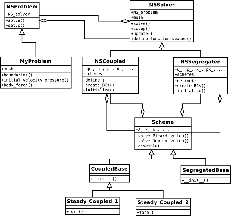
Figure 2: UML sketch of some problem, solver and scheme classes (with some of their methods and attributes) for laminar flow modeled by the Navier-Stokes equations. The arrows with triangular heads represent classes derived from the classes that they point towards. The arrows with diamond heads indicate that the class pointed to is part of the class that is pointing. For example, an NSSolver class contains a reference to an NSProblem class and an NSProblem class contains a reference to an NSSolver class.

5.2.2 Solver classes

Any problem class has a solver (NSSolver subclass), and any solver class has a reference back to the problem class. It may be necessary for several problem classes to share the same solver. The key action is calling problem.solve, where the default implementation in the superclass just calls the solver’s solve function. A problem-specific version of solve can alternatively be defined in the user’s problem class.

The setup method in the class NSSolver performs five important initialization steps: extracting the mesh from the problem class, defining function spaces, defining variational forms, initialization of velocity and pressure functions and defining boundary conditions. The definition of function spaces and forms is done in methods that must normally be overridden in subclasses, since these steps are usually tightly connected to the numerical method used to solve the equations. Here is an example of defining function spaces for $u$, $p$, the compound function $({\mbox{\boldmath$u$}},p)$, as well as a tensor function space for computing the strain rate tensor:

    def define_function_spaces(self):        u_degree = self.prm[’degree’][’velocity’’]        p_degree = self.prm[’degree’][’pressure’]        self.V = VectorFunctionSpace(self.mesh, ’Lagrange’, u_degree)        self.Q = FunctionSpace(self.mesh, ’Lagrange’, p_degree)        self.VQ = self.V*self.Q  # mixed element        # Symmetric tensor function space for strain rates Sij        d = self.mesh.geometry().dim()  # space dim.        symmetry = dict(((i,j), (j,i)) for i in range(d) \                        for j in range(d) if i > j)        self.S = TensorFunctionSpace(self.mesh, ’Lagrange’, u_degree,                                     symmetry=symmetry)We will sometimes show code like the above without further explanation. The purpose is to outline possibilities and to provide a glimpse of the size and nature of the code needed to realize certain functionality in FEniCS and Python.

Consider the coupled numerical method from Section 4.1 for the Navier-Stokes equations, combined with Picard or Newton iteration and under-relaxation. We need finite element functions for the most recently computed approximations ${\mbox{\boldmath$u$}}_{-}$ and $p_{-}$, named self.u_ and self.p_ in the code. Because we wish to solve a nonlinear system for $({\mbox{\boldmath$u$}},p$), there is a need for the compound function self.up_ with a vector $x_{-}$ (self.x_) of degrees of freedom. This vector should share storage with the vectors of ${\mbox{\boldmath$u$}}_{-}$ and $p_{-}$. The update of self.x_ is based on relaxing the solution of the linear system with the old value of self.x_. Taking into account that $u$ and $p$ are vector and scalar functions, respectively, normally approximated by different types of finite elements, it is not trivial to design a clean code (especially not in C and Fortran 77, which are the dominant languages in the CFD). There is, fortunately, convenient support for working with functions and their vectors on individual and mixed spaces in FEniCS. A typical initialization of data structures is a shared effort between the superclass and the derived solver class. The superclass is responsible for collecting all relevant information from the problem, whereas the derived class initializes solver specific functions and hooks up with appropriate schemes:

class NSSolver:    ...    def setup(self):        self.NS_problem.setup(self)        self.mesh = self.NS_problem.mesh        self.define_function_spaces()        self.u0_p0 = self.NS_problem.initial_velocity_pressure()        self.boundaries = self.NS_problem.boundaries()        self.f = self.NS_problem.body_force()        self.nu = Constant(self.NS_problem.prm[’viscosity’])class NSCoupled(NSSolver)    ...    def setup(self):        NSSolver.setup(self)        VQ = self.VQ        (self.v, self.q) = TestFunctions(VQ)        self.up = TrialFunction(VQ)        (self.u, self.p) = ufl.split(self.up)        self.bcs = self.create_BCs(self.boundaries)        self.up_ = Function(VQ)        self.u_, self.p_ = self.up_.split()        self.x_ = self.up_.vector()        self.initialize(self.u0_p0.vector())        self.schemes = {’NS’: None, ’parameters’: []}        self.define()Creating self.up_ as a $({\mbox{\boldmath$u$}},p)$ function on $V\times Q$ and then splitting this compound function into parts on $V$ and $Q$, gives two references (“pointers” in C-style terminology): self.u_ to ${\mbox{\boldmath$u$}}_{-}$ and self.p_ to $p_{-}$. Whenever we update self.u_ or self.p_, self.up_ is also updated, and vice versa. Similarly, updating self.x_ in-place updates the values of the compound function self.up_ and its parts self.u_ and self.p_, since memory is shared. That is, we can work with $u$ or $p$ or $({\mbox{\boldmath$u$}},p)$, or their corresponding degrees of freedom vectors interchangeably, according to what is the most appropriate abstraction for a given operation. The generalization to a more complicated system of vector and scalar PDEs is straightforward.

The self.nu variable deserves a comment. For laminar flow, self.nu will typically be a Constant(self.NS_problem.prm[’viscosity’]), but in turbulence computations self.nu must refer to this constant plus a finite element representation of $\nu_{T}$ (see equation (15)). This is accomplished by a simple (re)assignment in the turbulent case. Computer languages with static typing would here need some parameterization of the type, when it changes from Constant to Constant + Function. Normally, this requires nontrivial object-oriented or generative programming in C++, but dynamic typing in Python makes an otherwise complicated technical problem trivial. Especially in PDE solver frameworks, new logical combinations are needed, as is the ability to let variables point to new objects since this leads to simple and compact code. The corresponding code in C++, Java, or C# would usually introduce extra classes to help “simulate” flexible references, resulting in frameworks with potentially a large number of classes.

5.2.3 Iteration schemes

Subclasses of the Scheme class hierarchy implement specific linearized variational forms that can be combined in solver classes to implement various discretizations of the governing system of PDEs. As mentioned, reuse of common variational forms, their matrices and preconditioners, as well as encapsulation of optimization tricks are the primary reasons for introducing the Scheme hierarchy. Here is one class for the variational forms associated with a fully coupled NS solver:

class CoupledBase(Scheme):    def __init__(self, solver, unknown):        Scheme.__init__(self, solver, unknown, ...)        form_args = vars(solver).copy()        if self.prm[’iteration_type’] == ’Picard’:            F = self.form(**form_args)            self.a, self.L = lhs(F), rhs(F)        elif self.prm[’iteration_type’] == ’Newton’:            form_args[’u_’], form_args[’p_’] = solver.u, solver.p            up_, up = unknown, solver.up            F = self.form(**form_args)            F_ = action(F, function=up_)            J_ = derivative(F_, up_, up)            self.a, self.L = J_, -F_Subclasses of Scheme hold the forms a and L that are needed for forming the linear system associated with the variational form represented by the class. Typically, a method form (in a subclass of CoupledBase) defines this variational form, here stored in the F variable, and then the a and L parts are extracted. Note that a full Newton method is easily formulated, thanks to UFL’s support for automatic differentiation. First, we define the nonlinear variational form F by substituting the variable u_ in the scheme by the trial function solver.u (similar for the pressure). Second, the right-hand side is generated by applying the nonlinear form F as an action on the most recently computed unknown function (i.e., the trial function is replaced by up_, which is solver.up_). Then we can compute the Jacobian of the nonlinear form in one line.

Besides defining and storing the forms self.a and self.L, a scheme class also assembles the associated matrix self.A and vector self.b, and solves the system for the solution self.x. The latter variable simply refers to the vector storage of the solver.up_ Function. That is, the solver is responsible for creating storage for the primary unknowns and derived quantities, while scheme classes create storage for the matrix and right-hand side associated with the solution of the equations implied by the variational forms.

Subclasses of CoupledBase provide the exact formula for the variational form through the form method. Here is an example of a fully implicit scheme:

class Steady_Coupled_1(CoupledBase):    def form(self, u, v, p, q, u_, nu, f, **kwargs):        return inner(v, dot(grad(u), u_))*dx \            + nu*inner(grad(v), grad(u)+grad(u).T)*dx - inner(v, f)*dx \            - inner(div(v), p)*dx - inner(q, div(u))*dxThe required arguments are passed to form as a namespace dictionary containing all variables in the solver (see the constructor of CoupledBase where form is called). Alternatively, we may list only those variables that are needed as arguments to the form method, at the cost of extensive writing if numerous parameters are needed in the form (as in RANS models). Note that the **kwargs argument absorbs all the extra uninteresting variables in the call that do not match the names of the positional arguments. Yet, there is no additional overhead involved, because the **kwargs dictionary is simply a pointer to the solver’s namespace.

Picard and Newton variants can both employ the form shown above – the difference is simply the u_ argument (${\mbox{\boldmath$u$}}_{-}\cdot\nabla{\mbox{\boldmath$u$}}$ versus ${\mbox{\boldmath$u$}}\cdot\nabla{\mbox{\boldmath$u$}}$). Setting the u_ variable in the namespace dictionary form_args to solver.u instead of solver.u_, makes the first term evaluate to the nonlinear form inner(v, dot(grad(u), u))*dx.

An explicit scheme, utilizing only old velocities in the convection term, is implemented similarly:

class Steady_Coupled_2(CoupledBase):    def form(self, u, v, p, q, u_, nu, f, **kwargs):       if type(solver.nu) is Constant and \           self.prm[’iteration_type’] == ’Picard’:           self.prm[’reassemble_lhs’] = False       return inner(v, dot(grad(u_), u_))*dx \           + nu*inner(grad(v), grad(u)+grad(u).T)*dx - inner(v, f)*dx \           - inner(div(v), p)*dx - inner(q, div(u))*dxThe convective term for the explicit scheme is different from that for the implicit scheme, but we also flag that in a Picard iteration, for constant viscosity, the coefficient matrix does not change since the convective term only contributes to the right-hand side, implying that reassembly can be avoided. Such optimizations are key features of classes in the Schemes hierarchy.

In the real implementation of our framework, the convective term is evaluated by a separate method where one can choose between several alternative formulations of this term. Also, stabilization terms, like shown in (26), can be added in the form method.

The solver class, which one normally would assign the task of defining variational forms, now refers to subclass(es) of Scheme for defining appropriate forms and also for assembling matrices and solving linear systems. The solver class holds the system of equations, and each individual equation is represented as a scheme class. A coupled solver adds the necessary schemes to a schemes dictionary as part of the setup procedures:

class NSCoupled(NSSolver):    ...    def define(self):        # Define a Navier-Stokes scheme        classname = self.prm[’time_integration’] + ’_Coupled_’ + \                    str(self.prm[’scheme_number’][’velocity’])        self.schemes[’NS’] = eval(classname)(self, self.up_)User-given parameters are used to construct the appropriate name of the subclass of Scheme that defines the relevant form. With eval we can turn this name into a living object, without the usual if or case statements in factory functions that would be necessary in C, C++, Fortran, and Java.

5.2.4 Derived quantities

Derived quantities, such as the strain rate and stress tensors, can be computed once $u$ and $p$ are available. For a low-Reynolds turbulence model, Table 1 lists numerous quantities that must be derived from the primary unknowns in the system of PDEs. Some of the derived quantities can be computed from the primary unknowns without any derivatives, e.g., $\nu_{T}=C_{\mu}f_{\mu}k^{2}/\epsilon$ with $f_{\mu}$ being an exponential function of $Re_{T}\sim k^{2}/\epsilon$. One can either project the expression of $\nu_{T}$ onto a finite element space or one can compute the degrees of freedom of $\nu_{T}$ directly from the degrees of freedom of $k$ and $\epsilon$. Other derived quantities, such as $D$ in Table 1, involve derivatives of the primary unknowns. These derivatives are discontinuous across cell facets, and when needed in some variational form, we can either use the quantity’s form as it is, or we may choose to first project the quantity onto a finite element space of continuous functions and then use it in other contexts.

To effectively define and work with the large number of derived quantities in RANS models, we need a flexible code construction where we essentially write the formula defining a derived quantity $Q$ and then choose between three ways of utilizing the formula: we may (i) project $Q$ onto a space $V$, (ii) use the formula for $Q$ directly in some variational form, or (iii) compute the degrees of freedom of $Q$, by applying the formula to each individual degree of freedom, for efficiently creating a finite element function of $Q$. A class DerivedQuantity is designed to hold the definition of a derived quantity and to apply it in one of the three aforementioned ways. In some solver class (like NSCoupled) we can define the computation of a derived quantity, say the strain rate tensor $S$, by

Sij = DerivedQuantity(solver=self, name=’Sij’, space=self.S,      formula=’strain_rate(u_)’, namespace=ns, apply=’project’)The formula for $S$ makes use of a Python function

def strain_rate(u):    return 0.5*(grad(u) + grad(u).T)Alternatively, the formula argument could be the expression inside the strain_rate function (with u replaced by u_). We may nest functions for defining derived quantities, e.g., the stress tensor could be defined as formula=’stress(u_, p_, nu)’ where

def stress(u, p, nu):    d = u.cell().d  # no of space dimensions    return 2*nu*strain_rate(u) - p*Identity(d)The namespace argument must hold a namespace dictionary in which the string formula is going to be evaluated by eval. It means, in the present example, that ns must be a dictionary defining u_, strain_rate, and other objects that are needed in the formula for the derived quantity. A quick construction of a common namespace for most purposes is to let ns be the merge of vars(self) (all attributes in the solver) and globals() (all the global functions and variables in the solver module).

The apply argument specifies how the formula is applied: for projection (’project’), direct computations of degrees of freedom (’compute_dofs’), or plain use of the formula (’use_formula’). Other arguments are optional and may specify how to solve the linear system arising in projection, how to under-relax the projected quantity, etc. When this information is lacking, the DerivedQuantity class looks up missing information in the parameters (prm) dictionary in the solver class.

A formula for a derived quantity may involve previously defined quantities. Therefore, since ordering is key, a solver will typically collect its definitions of derived quantities in an ordered list.

A DerivedQuantity object is a special kind of a Scheme object, and therefore naturally derives from Scheme. The inner workings depend on quite advanced Python coding, but yield great flexibility. The fundamental idea is to specify the formula as a string, and not a UFL expression, because such a string can be evaluated by eval in different namespaces, yielding different results. Say we have a DerivedQuantity object with some formula ’k**2’. With a namespace ns where k is tied to an object k of type TrialFunction, ns[’k’] = k, the call eval(formula, ns) will turn the string into a UFL expression where k is an unknown finite element function. On the other hand, with ns[’k’] = k_, k_ being an already computed finite element function, the eval call turns ’k**2’ into ’k_**2, which yields a known right-hand side in a projection or a known source term in a variational form. Moreover, ns[’k’] = k.vector().array() associates the variable k in the formula with its array of the degrees of freedom, and the eval call will then lead to squaring this array. The result can be inserted into the vector of degrees of freedom of a finite element field to yield a more efficient computation of the field than the projection approach.

Derived quantities that are projected may need to overload the default boundary conditions through the create_BCs method. The DerivedQuantity class is by default set to enforce assigned boundary conditions on walls, whereas a subclass DerivedQuantity_NoBC does not. The latter is in fact used by the implemented shear stress Sij, since the velocity gradient on a wall in general will be unknown.

Especially in complex mathematical models with a range of quantities that are defined as formulae involving the primary unknowns, the DerivedQuantity class helps to shorten application code considerably and at the same time offer flexibility with respect to explicit versus implicit treatment of formulae, projection of quantities for visualization, etc.

5.2.5 Solution of linear systems

The Scheme classes are responsible for solving the linear system associated with a form. Since the Picard and Newton methods have different unknowns in the linear system ($u$ and $p$ versus corrections of $u$ and $p$), a general solve method is provided for each of them. The Picard version with under-relaxation reads

def solve_Picard_system(self, assemble_A, assemble_b):    for name in (’A’, ’x’, ’b’, ’bcs’):        exec str(name + ’ = self.’ + name)  # strip off self.    if assemble_A: self.assemble(A)    if assemble_b: self.assemble(b)    [bc.apply(A, b) for bc in bcs]  # boundary conditions modify A, b    self.setup_solver(assemble_A, assemble_b)    x_star = self.work    x_star[:] = x[:]  # start vector for iterative solvers    self.linear_solver.solve(A, x_star, b)    # relax: x = (1-omega)*x + omega*x_star = x + omega*(x_star-x)    omega = self.prm[’omega’]    x_star.axpy(-1., x); x.axpy(omega, x_star)    self.update()    return residual(A, x, b), x_starNote how we first strip off the self prefix (by loading attributes into local variables) to make the code easier to read and closer to the mathematical description. This trick is frequently used throughout our software to shorten the distance between code and mathematical expressiveness. The linear system is assembled only if the previously computed A or b cannot be reused. Similarly, if A can be reused, the factorization or preconditioner in a linear solver can also be reused (the setup_solver method will pass on such information to the linear solver). After the linear solver has computed the solution x_star, the new vector of velocities and pressures, x, is computed by relaxation. For this purpose we use the classical “axpy” operation: $y\leftarrow ax+y$ ($a$ is scalar, $x$ and $y$ are vectors). Since “axpy” is an efficient operation (carried out in, e.g., PETSc if that is the chosen linear algebra backend for FEniCS), we rewrite the usual relaxation update formula to fit with this operation. The in-place update of x through the axpy method is essential when x has memory shared with several finite element functions, as explained earlier. The returned values are the solution of one iteration, the corresponding residual and the difference between the previous and the new solution (reflected by x_star after its axpy update).

The solution of a linear system arising in Newton methods requires a slightly different function, because we solve for a correction vector, and the residual is the right-hand side of the system.

def solve_Newton_system(self, *args):    for name in (’A’, ’x’, ’b’, ’bcs’):        exec str(name + ’ = self.’ + name)    self.assemble(A)    self.assemble(b)    [bc.apply(A, b, x) for bc in bcs]    dx =self. work  # more informative name    dx.zero()    self.linear_solver.solve(A, dx, b)    x.axpy(self.prm[’omega’], dx)    self.update()    return norm(b), dxThe dummy arguments *args are included in the call (but never used) so that solve_Picard_system and solve_Newton_system can be called with the same set of arguments. A simple wrapper function solve will then provide a uniform interface to either the Picard or Newton version for creating and solving a linear system:

def solve(self, assemble_A=None, assemble_b=None):    return eval(’self.solve_%s_system’ % self.prm[’iteration_type’])\               (assemble_A, assemble_b)With this solve method, it is easy to write a general iteration loop to reach a steady state solution. This loop is independent of whether we use the Newton or Picard method, or how we avoid assembly and reuse matrices and vectors:

def solve_nonlinear(scheme, max_iter=1, max_err=1e-8, update=None):    j = 0; err = 1E+10    scheme.info = {’error’: (0,0), ’iter’: 0}    while err > max_err and j < max_iter:        res, dx = scheme.solve(scheme.prm[’reassemble_lhs’],                               scheme.prm[’reassemble_rhs’])        j += 1        scheme.info = {’error’: (res, norm(dx)), ’iter’: j}        if scheme.prm[’echo’]: print scheme.info        err = max(scheme.info[’error’])        if update: update()    return scheme.infoThe scheme object is a subclass of Scheme that has the solve method listed above. The update argument is usually some method in the solver object that updates data structures of interest, which could be some derived quantity (e.g., $S$ and $\nabla\cdot{\mbox{\boldmath$u$}}$). It can also be used to plot or save intermediate results between iterations. Note that scheme also has an update method that is called at the end of solve_Picard/Newton_system. The scheme.update method is often used to enforce additional control over x, e.g., for k_ by ensuring that it is always larger than zero.

A useful Python feature is the ability to define new class attributes whenever appropriate, and is used in the preceding snippet for storing information about the iteration in scheme.info. This presents the possibility of adding new components to a framework to dynamically increase functionality. Simple code may remain simple, even when extensions are required for more complex cases, since extensions can be added when needed at run-time by other pieces of the software.

In a classical object-oriented C++ design, the stand-alone solve_nonlinear function would naturally be a method in an NS solver superclass. However, reuse of this generic iteration function to solve other equations then forces those equations to have their solvers as subclasses in the NS hierarchy. Also, the shown version of solve_nonlinear is very simple, checking only the size of the norms of the residual for convergence. More sophisticated stopping criteria can be implemented and added trivially. Alternatively, a user may want a tailored solve_nonlinear function. This is trivially accomplished, whereas if the function were placed inside a class in a class hierarchy, the user would need to subclass that class and override the function. This approach connects the new function to a particular solver class, while a stand-alone function can be combined with any solver class from any solver hierarchy as long as the solver provides certain attributes and methods. The same flexibility can be achieved by generative programming in C++ via templates.

The solve methods in solver classes will typically make use of solve_nonlinear or variants of it for performing the solve operation.

5.3 Reynolds-averaged Navier-Stokes models

The class NSSolver and its subclasses are designed to be used without any turbulence model, but with the possibility of having a variable viscosity. Since RANS models are implemented separately in their own classes, we need to decide on the relation between NS solver classes and RANS solver classes. There are three obvious approaches: (1) let a RANS model be a subclass of an NS solver class; (2) let a RANS model have a reference to an instance of an NS solver; or (3) let a RANS solver only define and solve RANS equations, and then use a third class to couple NS and RANS classes. We want maximum flexibility in the sense that any solution method for the NS equations can in principle be used with any turbulence model. Approach (1), with subclassing RANS models, ties a RANS model to a particular NS class and thus limits flexibility. With approaches (2) and (3), the user selects any RANS model and any NS solution method. Since a RANS model is incomplete without an NS solver, we prefer approach (2).

Mirroring the structure of the NS solver, RANS solvers have a superclass TurbSolver, while the TurbProblem acts as superclass for the turbulence problems. Any turbulence problem contains an NSProblem class for defining the basic flow problem, plus parameters related to turbulence PDEs and their solution methods. Figure 3 sketches the relationships between some of the classes to be discussed in the text.

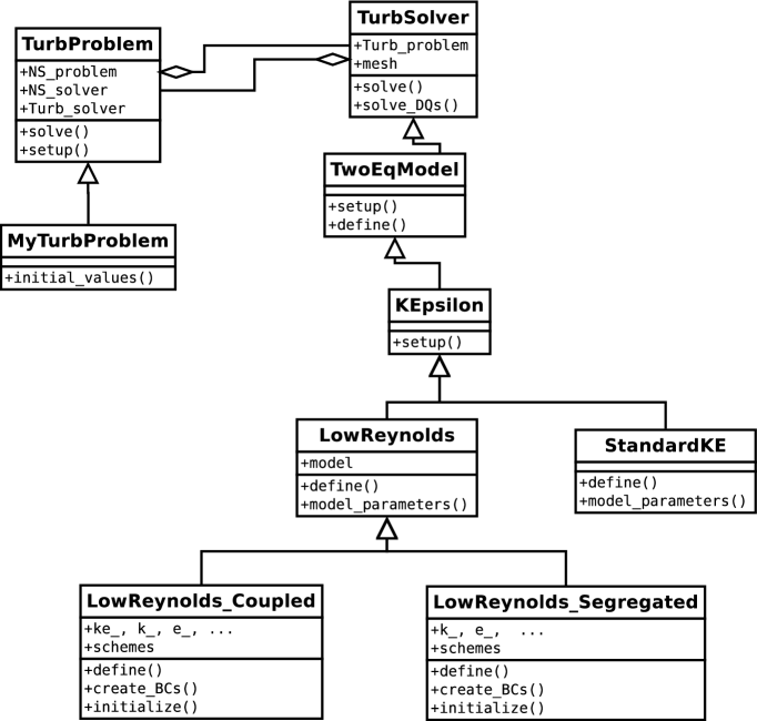
Figure 3: Sketch of a few problem and solver classes (with some of their methods and attributes) for turbulent flow modeled by RANS.

5.3.1 Required functionality

RANS modeling poses certain numerical challenges that a software system must be able to deal with in a flexible way. It must be easy to add new PDEs and combine PDEs with various constitutive relations to form new models or variations on classical ones. Due to the nonlinearties in turbulence PDEs, the degree of implicitness when designing an effective and robust iteration method is critical. We wish to make switching between implicit and explicit treatments of terms in an equation straightforward, thereby offering complete control over the linearization procedure. Key is the flexibility to construct schemes. This is made possible in part by automatic symbolic differentiation, which can be applied selectively to different terms.

5.3.2 Creating a turbulent flow problem

Solving a turbulent flow problem is a matter of extending the code example from Section 5.2.1. We make use of the same MyProblem class for defining a mesh, etc., but for a turbulent flow we might want to initialize the velocity and pressure differently. For this purpose we overload the initial_velocity_pressure method in MyProblem. A subclass of TurbProblem must be defined to set initial conditions for the turbulence equations and supply the solver with the correct boundary values (the boundaries are already supplied by MyProblem). The creation of problem and solver classes, and setting of parameters through predefined dictionaries in the cbc.rans modules, may look as follows for a specific flow case:

import cbc.rans.nsproblems as nsproblemsimport cbc.rans.nssolvers as nssolversimport cbc.rans.turbproblems as turbproblemsimport cbc.rans.turbsolvers as turbsolversclass MyProblem(nsproblems.MyProblem):    """Overload initialization of velocity/pressure."""    def initial_velocity_pressure(self):        ...class MyProblemTurb(TurbProblem):    ...nsproblems.parameters.update(Nx=10, Ny=10)turbproblems.parameters.update(Model=’Chien’, Re_tau=395.)nsproblems.parameters.update(turbproblems.parameters)NS_problem = MyProblem(nsproblems.parameters)nssolvers.parameters = recursive_update(nssolvers.parameters,          dict(degree=dict(velocity=2, pressure=1)))NS_solver  = nssolvers.NSCoupled(NS_problem, nssolvers.parameters)NS_solver.setup()problem = MyTurbProblem(NS_problem, turbproblems.parameters)turbsolvers.parameters.update(iteration_type=’Picard’, omega=0.6)solver = turbsolvers.LowReynolds_Coupled(problem,                                         turbsolvers.parameters)solver.setup()problem.solve(max_iter=10)

5.3.3 Turbulence model solver classes

The TurbSolver class has a relation to the TurbProblem class that mimics the relation between NSSolver and NSProblem. Moreover, TurbSolver needs an object in the NSSolver hierarchy to solve the NS equations during the iterations of the total system of PDEs. As mentioned in Section 5.2.2, the self.nu variable in an NS solver must now point to the finite element function representing $\nu+\nu_{T}$ in the RANS model.

We have two basic choices when implementing a RANS model, either to develop a specific implementation tailored to a particular model, or to make a general toolbox for a system of PDEs. The former approach is exemplified in the next section for a $k$–$\epsilon$ model, while the latter is discussed in Section 5.3.5. To implement a $k$–$\epsilon$ model, one naturally makes a subclass KEpsilon in the TurbSolver hierarchy. Some tasks are specific to the $k$–$\epsilon$ model in question and are better distributed to subclasses like StandardKE or LowReynolds. The choice between the three low-Reynolds models is made in LowReynolds whereas some of the data structures are defined in subclasses for either a coupled or segregated approach. In Figure 3 we also sketch the possibility of having a TwoEquationModel class with functionality common to all two-equation models.

A setup method defines the data structures and forms needed for a solution of the $k$ and $\epsilon$ equations. The code is similar to the setup method for the NS solver classes. Definition of the specific forms is performed through the Scheme class hierarchy. Any solver class has a schemes attribute which holds a dictionary of all the needed schemes. A coupled low-Reynolds model will have a scheme ’ke’ for solving the $k$ and $\epsilon$ equations, and a segregated model will have schemes ’k’ and ’e’ for the individual $k$ and $e$ equations. In addition, there is a list of schemes for all the derived quantities, such as $\nu_{T}$, $f_{\mu}$, $f_{2}$, etc.

All scheme objects are declared through the method define, which typically will be called as the final task of the setup method. It is possible to change the composition of scheme objects at run-time and simply rerun define, without having to reinitialize function spaces, test and trial functions, and unknowns.

5.3.4 Defining a specific two-equation model

The equations of all turbulence models are defined by subclasses of Scheme and can be transparently used with Picard or Newton iterations, as previously exemplified for a coupled NS solver in Section 5.2.3. Here is an outline of a coupled $k$-$\epsilon$ model:

class KEpsilonCoupled(Scheme):    def __init__(self, solver, unknown):        Scheme.__init__(self, solver, ...)        form_args = vars(solver).copy()        if self.prm[’iteration_type’] == ’Picard’:            F = self.form(**form_args)            self.a, self.L = lhs(F), rhs(F)        elif self.prm[’iteration_type’] == ’Newton’:            form_args[’k_’], form_args[’e_’] = solver.k, solver.e            F = self.form(**form_args)            ke_, ke = unknown, solver.ke            F_ = action(F, function=ke_)            J_ = derivative(F_, ke_, ke)            self.a, self.L = J_, -F_As in the CoupledBase constructor for the NS schemes, we send all attributes in the solver class as keyword arguments to the form methods. Most of these arguments are never used and are absorbed by a final **kwargs argument, but the number of variables needed to define a form is still quite substantial:

class Steady_ke_1(KEpsilonCoupled):    def form(self, k, e, v_k, v_e,  # Trial and TestFunctions                   k_, e_, nut_, u_, Sij_, E0_, f2_, D_, # Functions/forms                   nu, e_d, sigma_e, Ce1, Ce2, **kwargs): # Constants        Fk = (nu + nut_)*inner(grad(v_k), grad(k))*dx \            + inner(v_k, dot(grad(k), u_))*dx \            - 2.*inner(grad(u_), Sij_)*nut_*v_k*dx \            + (k_*e*e_d + k*e_*(1. - e_d))*(1./k_)*v_k*dx + v_k*D_*dx        Fe = (nu + nut_*(1./sigma_e))*inner(grad(v_e), grad(e))*dx \            + inner(v_e, dot(grad(e), u_))*dx \            - (Ce1*2.*inner(grad(u_), Sij_)*nut_*e_ \            - f2_*Ce2*e_*e)*(1./k_)*v_e*dx - E0_*v_e*dx        return Fk + FeVariants of this form, with different linearizations, are defined similarly. By a proper construction of class names, based on user-given parameters, the factory function for creating the right scheme object can be coded in one line with eval, as exemplified in NSCoupled.define. On the contrary, registering a user-defined scheme in a library coded in a statically typed language (Fortran, C, C++, Java, or C#) requires either an extension of the many switch or if-else statements of a factory function in the library, or sophisticated techniques to overcome the constraints of static typing.

The turbulence solver class mimics most of the code presented for the NSCoupled class. That is, we must define function spaces for $k$ and $\epsilon$, and a compound (mixed) space for the coupled system. The primary unknown in this system, called ke, and its Function counterpart ke_, are both defined similarly to up and up_ in class NSCoupled. A considerable extension, however, is the need to define all the parameters and quantities that enter the turbulence model. For the form method above to work, these quantities must be available as attributes fmu_, f2_, etc., in the solver class so that the form_args dictionary contains these names and can feed them to the form method. Details on the definitions of turbulence quantities will appear later.

5.3.5 General systems of turbulence PDEs

The briefly described classes for the $k$-$\epsilon$ model are very similar to the corresponding classes for the NS schemes, and in fact to all other turbulence models. The only difference is the name of the primary unknowns, their corresponding variable names in the solver class and their coupling. An obvious idea is to parameterize the names of the primary unknowns in turbulence models and create code that is common. This makes the code for adding a new model dramatically shorter.

For the solution of a general system of PDEs, we introduce a list, here called system_composition, containing the names of the primary unknowns in the system and how they are grouped into subsystems that are to be solved simultaneously. For example, [[’k’, ’e’]] defines only one subsystem consisting of the primary unknowns k and e to be solved for in a coupled fashion (see LowReynolds_Coupled in Figure 4). The list [[’k’], [’e’]] defines two subsystems, one for k and one for e, and is the relevant specification for a segregated formulation of a $k$–$\epsilon$ model (e.g., LowReynolds_Segregated in Figure 4). A fully coupled $v^{2}$-$f$ model ¹⁸ is specified by the list [[’k’, ’e’, ’v2’, ’f’]], while the common segregated strategy of solving a coupled $k$-$\epsilon$ system and a coupled $v^{2}$-$f$ system is specified by [[’k’, ’e’], [’v2’, ’f’]]. Using the system_composition list and a few simple naming rules, we will now illustrate how all tasks of creating relevant function spaces, data structures, boundary conditions and even initialization, can be fully automated in the superclass TurbSolver for most systems. Figure 4 shows the class hierarchy where the superclass TurbSolver performs most of the work and the individual models need merely to implement bare necessities like model_parameters and define to set up the schemes dictionary.

From the system_composition list we can define the name of a subsystem as a simple concatenation of the unknowns in the subsystem, e.g., ke for a coupled $k$-$\epsilon$ model and kev2f for a fully coupled $v^{2}$-$f$ model. We need to create unknowns for these concatenated names as well as Functions for the names and all individual unknowns. This can be done compactly as shown below.

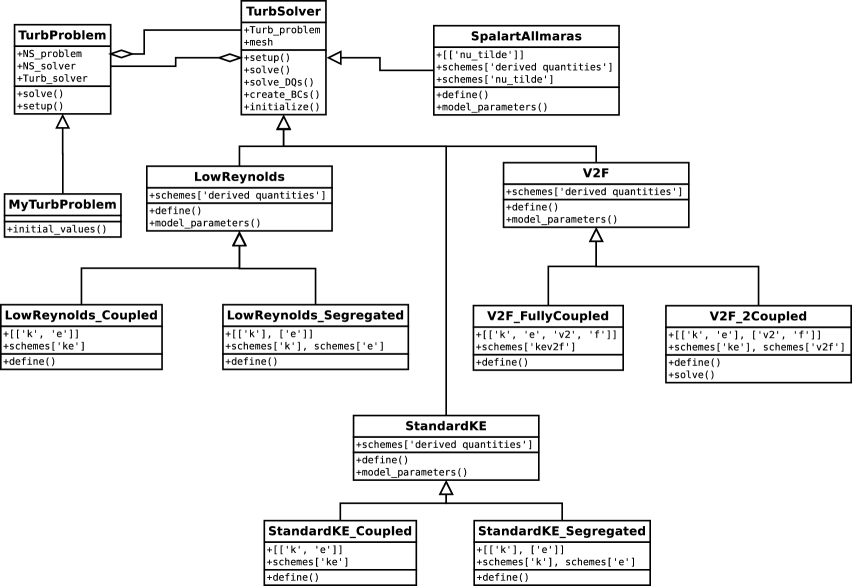
Figure 4: Sketch of a modified and extended collection of turbulence problem and solver classes. For better illustration, the lowest level of solver classes show the value of the system composition attribute as lists.

We will now go into details of the abstract code required to automate common tasks. Dictionaries, indexed by the name of an unknown (a single unknown such as k, or a compound name for the unknown in a subsystem such as ke), are introduced: V for the function spaces, v for the test functions, q for the trial functions, q_ for the Function objects holding the last computed approximation to q, q_1 for the Function objects holding the unknowns at the previous time step (and q_2, q_3, for older time steps, if necessary), and q0 for the initial conditions. For example, q[’e’] holds the trial function for $\epsilon$ in a $k$-$\epsilon$ model, v[’e’] is the corresponding test function, V[’e’] is the corresponding function space, q[’ke’] holds the trial function (in a space V[’ke’]) for the compound unknown ($k$, $\epsilon$) in a coupled $k$-$\epsilon$ formulation, q_[’ke’] (in a space V[’ke’]) holds the corresponding computed finite element function, and so on.

The constructor takes the system composition and creates lists of all names of all unknowns and the names of the subsystems:

class TurbSolver:    def __init__(self, system_composition, problem, parameters):        self.system_composition = system_composition        self.system_names = [];  self.names = []        for sub_system in self.system_composition:            self.system_names.append(’’.join(sub_system) )            for name in sub_system:                self.names.append(name)Defining the function spaces for each unknown and each compound unknown in subsystems is done by a dict comprehension:

    def define_function_spaces(self):        mesh = self.Turb_problem.NS_problem.mesh        self.V = {name: FunctionSpace(mesh, ’Lagrange’,                        self.prm[’degree’][name])                  for name in self.names + [’dq’]}        for sub_sys, sys_name in \            zip(self.system_composition, self.system_names):            if len(sub_sys) > 1:  # more than one PDE in the system?                self.V[sys_name] = MixedFunctionSpace(                    [self.V[name] for name in sub_sys])For a coupled $k$-$\epsilon$ model, the first assignment to self.V creates the spaces self.V[’k’], self.V[’e’] and self.V[’dq’], while the next for loop creates the mixed space self.V[’ke’]. The self.V[’dq’] object holds the space for derived quantities and is always added to the collection of spaces.

The test, trial, and finite element functions for the compound unknowns are readily constructed by:

    def setup_subsystems(self):        V, sys_names, sys_comp = \               self.V, self.system_names, self.system_composition        q   = {name: TrialFunction(V[name]) for name in sys_names}        v   = {name: TestFunction(V[name]) for name in sys_names}        q_  = {name: Function(V[name]) for name in sys_names}The quantities corresponding to the individual unknowns are obtained by splitting objects for compound unknowns. Typically,

        for sub_sys, sys_name in zip(sys_comp, sys_names):            if len(sub_sys) > 1:  # more than one PDE in the system?                q_.update({sub_sys[i]: f[i] \                           for i, f in enumerate(q_.split())}with a similar splitting of q, v, etc. Finally, these dictionaries are stored as class attributes:

        self.v = v; self.q = q; self.q_ = q_It is also convenient to create solver attributes with the same names as the keys in these dictionaries. That is, in a coupled $k$-$\epsilon$ model we make the short form self.k_ for self.q_[’k’], v_ke for self.v[’ke’], and similarly:

        for key, value in v .items(): setattr(self, ’v_’+key, value)        for key, value in q .items(): setattr(self, key, value)        for key, value in q_.items(): setattr(self, key+’_’, value)A dictionary self.x_ for holding the unknown vectors in the various linear systems are created in a similar way. To summarize, the ideas of the solver classes for NS problems and specific turbulence problems are followed, but unknowns are parameterized by names in dictionaries, with these names as keys, to hold the key objects. Class attributes based on the names refer to the dictionary elements, so that a solver class has attributes for trial and test functions, finite element functions, etc., just as in the NS solver classes. These class attributes are required when subclasses of Scheme define variational forms by sending solver attributes to a scheme method (see Sections 5.2.3 and 5.3.4). For example, when a scheme method needs a parameter e_ in the form, the object solver.e_ is sent as parameter (solver being the solver object), and this object is actually solver.q_[’e’] as created in the code segments above, perhaps by splitting the compound function solver.q_[’ke’] into its subfunctions.

With the names of the unknown parameterized, it becomes natural to also create common code for the scheme classes associated with turbulence models. We introduce a subclass TurbModel of Scheme that carries out the tasks shown for the KEpsilonCoupled class above, but now for a general system of PDEs:

class TurbModel(Scheme):    def __init__(self, solver, sub_system):        sub_name = ’’.join(sub_system)        Scheme.__init__(self, solver, sub_system, ...)        form_args = vars(solver).copy()        if self.prm[’iteration_type’] == ’Picard’:            F = self.scheme(**form_args)            self.a, self.L = lhs(F), rhs(F)        elif self.prm[’iteration_type’] == ’Newton’:            for name in sub_system:                # switch from Function to TrialFunction:                form_args[name+’_’] = solver.q[name]            F = self.scheme(**form_args)            u_ = solver.q_[sub_name]            F_ = action(F, function=u_)            u = solver.q[sub_name]            J_ = derivative(F_, u_, u)            self.a, self.L = J_, -F_Note that u denotes a general unknown (e.g., k, e, or ke) when automatically setting up the Newton system.

We now illustrate a specific subclass of a turbulence model. Considering a low-Reynolds model, we may create a subclass LowReynolds with a define method that sets up a list of necessary derived quantities to be computed in the NS solver ($S$, $E$) and all the derived quantities entering the low-Reynolds turbulence models (cf. Table 1). These depend on the specific model, whose name is available through the parameters dictionary in the turbulence problem class. The coding of the define method in class LowReynolds reads:

def define(self):    V = self.V[’dq’] # space for derived quantities    DQ, DQ_NoBC = DerivedQuantity, DerivedQuantity_NoBC  # short forms    NS = self.Turb_problem.NS_solver    model = self.Turb_problem.prm[’model’]    ns = dict(u_=NS.u_)    NS.schemes[’derived quantities’] = [        DQ(NS, ’Sij_’, NS.S, ’strain_rate(u_)’, ns),        ...]    self.Sij_ = NS.Sij_; self.d2udy2_ = NS.d2udy2_    ns = vars(self)   # No copy - derived quantities will be added    self.schemes[’derived quantities’] = dict(      LaunderSharma=lambda :[        DQ_NoBC(self, ’D_’, V, ’nu/2./k_*inner(grad(k_), grad(k_))’, ns),        DQ(self, ’fmu_’, V, ’exp(-3.4/(1. + (k_*k_/nu/e_)/50.)**2)’, ns),        DQ(self, ’f2_’ , V, ’1. - 0.3*exp(-(k_*k_/nu/e_)**2)’, ns),        DQ(self, ’nut_’, V, ’Cmu*fmu_*k_*k_*(1./e_)’, ns),        DQ(self, ’E_’  , V, ’2.*nu*nut_*dot(d2udy2_, d2udy2_)’, ns)],      JonesLaunder=lambda :[        DQ_NoBC(self, ’D_’, V, ’nu/2./k_*inner(grad(k_), grad(k_))’, ns),        DQ(self, ’fmu_’, V, ’exp(-2.5/(1. + (k_*k_/nu/e_)/50.))’, ns),        DQ(self, ’f2_’ , V, ’(1. - 0.3*exp(-(k_*k_/nu/e_)**2))’, ns),        DQ(self, ’nut_’, V, ’Cmu*fmu_*k_*k_*(1./e_)’, ns),        DQ(self, ’E_’  , V, ’2.*nu*nut_*dot(d2udy2_, d2udy2_)’, ns)],      Chien=lambda :[...]      )[model]()    TurbSolver.define(self)A significant number of constants are involved in the expressions for many of the derived quantities. These constants can be defined through dictionaries in another method:

    def model_parameters(self):        model = self.Turb_problem.prm[’model’]        self.model_prm = dict(Cmu=0.09, sigma_e=1.30,            sigma_k=1.0, e_nut=1.0, e_d = 0.5, f1 = 1.0)        Ce1_Ce2 = dict(            LaunderSharma=dict(Ce1=1.44, Ce2=1.92),            JonesLaunder= dict(Ce1=1.55, Ce2=2.0),            Chien=        dict(Ce1=1.35, Ce2=1.80))        self.model_prm.update(Ce1_Ce2[model])        # wrap in Constant objects:        for name in self.model_prm:            self.model_prm[name] = Constant(self.model_prm[name])        # store model_prm objects as class attributes:        self.__dict__.update(self.model_prm)Dictionaries are useful for storing the data, but in the scheme objects defining the forms we need a constant like Cmu as an attribute in the class, and this is accomplished by simply updating the __dict___ dictionary. Also note that constants should be wrapped in Constant objects if they enter variational forms written in UFL. That way constants may be changed without the need to recompile UFL forms.

Subclasses of LowReynolds define a segregated or a coupled scheme. For example,

class LowReynolds_Coupled(LowReynolds):    def __init__(self, problem, parameters):        LowReynolds.__init__(self, system_composition=[[’k’,’e’]],                             problem=problem, parameters=parameters)    def define(self):        LowReynolds.define(self)        classname = self.prm[’time_integration’] + ’_ke_’ + \                    str(self.prm[’scheme’][’ke’])        self.schemes[’ke’] = eval(classname)\                    (self, self.system_composition[0])Two actions are performed: definition of the subsystems to be solved (here the $k$-$\epsilon$ system); and creation of the scheme class that defines the variational form. If the user has set the solver parameters

turbsolvers.parameters[’time_integration’] =’Steady’turbsolvers.parameters[’scheme’][’ke’] = 1the classname variable becomes Steady_ke_1, and the corresponding class was shown in Section 5.3.4 (except that Steady_ke_1 is now derived from TurbModel and not the specialized KEpsilonCoupled).

A segregated solution approach to low-Reynolds models is implemented in a subclass LowReynolds_Segregated, where the system composition reads [[’k’],[’e’]], self.schemes[’k’] is set to some steady or transient scheme object for the $k$ equation and self.schemes[’e’] is set to a similar object defining the form in the $\epsilon$ equation.

Several turbulence models have already been implemented in cbc.rans using the generalized approach, and appear in Figure 4: the three low-Reynolds models as described, a standard $k$-$\epsilon$ model with wall functions, a Spalart-Allmaras one-equation model, a fully coupled $v^{2}$-$f$ model and a $v^{2}$-$f$ model divided into a coupled $k$-$\epsilon$ system and a coupled $v^{2}$-$f$ system. For each of these models, various scheme methods in subclasses of TurbModel define various linearizations.

Another class of models involve equations for each of the six components of the Reynolds stress tensor $R$. Minimal effort is required to make the creation of function spaces in TurbSolver work with vectors or even second order tensors since UFL has support for both vector and tensor-valued function spaces. In fact, a coupled scheme for computing all components of the Reynolds stress tensor can be expressed using computer code which mirrors the mathematical tensor notation, just as for the previously introduced scalar equations.

A particularly interesting application of the described framework is the implementation of structure-based turbulence models ²⁴, which introduce new turbulence measures and models, and lead to even larger larger systems of PDEs than found in more common Reynolds stress models. Such applications are in preparation by the authors.

6 Numerical examples

To demonstrate the framework, we consider two numerical examples. The complete computer code for the presented examples can be found in cbc.rans ⁸.

6.1 Fully developed turbulent channel

Statistically one-dimensional, fully developed channel flow between two parallel plates is used often in the development and verification of CFD codes. We will use this problem to investigate the impact of different approximate linearizations. The flow for the channel problem is characterized by a Reynolds number based on the friction velocity $u_{\tau}=(\sqrt{\nu\partial u_{x}/\partial y})_{\rm wall}$, where $u_{x}$ is the velocity tangential to the wall and $y$ is the wall normal direction. The friction-based Reynolds number is defined as $Re_{\tau}=u_{\tau}h/\nu$, where $h$ is half the channel height. Here $Re_{\tau}=395$, $u_{\tau}=0.05$ and $h=1$ are used. For this problem, ${\mbox{\boldmath$u$}}=\mathbf{0}$, $k=0$ and $\epsilon=0$ on walls, and periodic boundary conditions are applied at the inflow and outflow. The laminar flow profile is used for initial velocity field, and $k$ and $\epsilon$ are initially set to $0.01$.

We set up problem classes for the laminar and turbulent cases, as outlined in Section 5.3.2. A mesh with 50 elements in the wall normal direction for half the channel height and 10 elements in the stream-wise direction is used. Linear basis functions are used for all fields and the flow is driven by a constant pressure gradient. Due to the equal order or the velocity and pressure function spaces, the stabilized form (26) of the equations are used, with a constant $\tau=0.01$. Picard iterations are used with under-relaxation factors of 0.8 and 0.6 for the NS and turbulence equations, respectively. The problem class designed for the channel flow has to return initial values for $u$, $k$ and $\epsilon$. The problem class also defines two SubDomains that are used to identify the wall and the mapping between the periodic in- and outlets.

The first example concerns the linearization of the dissipation term $\epsilon$ in the $k$ equation (17). Since $\epsilon$ appears in the $k$ equation, an explicit treatment of $\epsilon_{-}$ may appear natural. However, an implicit treatment of $\epsilon$ will normally contribute to enhanced stability. Moreover, we also introduce a different implicit discretization through a weighting of $\epsilon_{-}k/k_{-}$ and $\epsilon$ in (41). This term is often used by segregated solvers as it adds terms to the diagonal entries of the coefficient matrix, which improves the condition number to the benefit of Krylov solvers. Here we will use a direct solver. The purpose is to investigate the impact of the weighting factor $e_{d}$ on the convergence behavior when solving the nonlinear equations. We remark that the weighted form (41) (see (41)) is of relevance only for a coupled solution procedure since $e_{d}\neq 0$ implies that $\epsilon$ is unknown in the $k$ equation.

The simulation of the channel problem for all models for a range of $e_{d}$ values is scripted and run by:

# Get relevant solvers and problemsnssolver = nssolvers.NSCouplednschannel = turbproblems.NS_channelturbchannel = turbproblems.channelturbsolver = turbsolvers.LowReynolds_Coupled# Redefine relevant parameters dictionariesprm_ns = nsproblems.parametersprm_turb = turbproblems.parametersprm_nssol = nssolvers.parametersprm_turbsol = turbsolvers.parametersprm_ns.update(dict(Nx=10, Ny=50))prm_nssol = recursive_update(prm_nssol,         dict(degree=dict(velocity=1), omega=0.8))prm_turbsol.update(omega=0.6)prm_turb.update(Re_tau=395, utau=0.05)# Loop over all models and e_dfor model in [’LaunderSharma’,’JonesLaunder’, ’Chien’]:    for e_d in linspace(0,1,5):        prm_turb.update(Model=model)        prm_ns.update(prm_turb)        NS_problem = nschannel(prm_ns)        NS_solver = nssolver(NS_problem, prm_nssol)        NS_solver.setup()        Problem = turbchannel(NS_problem, prm_turb)        Solver = turbsolver(Problem, prm_turbsol)        Solver.setup()        Solver.e_d = Constant(e_d)        Solver.define()        Problem.solve(max_iter=50, max_err=1e-12)        ... # Store results etc

Figure 5 shows the convergence response for the three low Reynolds number turbulence models discussed in Section 3. The fully coupled form using $e_{d}=1$ is the most efficient method for LaunderSharma and JonesLaunder, whereas it is unstable for Chiens model. The “segregated” form $\epsilon_{-}k/k_{-}$ ($e_{d}=0$) is least efficient, whereas a blend of both forms seems to be optimal as a default option for all models. It is interesting to note that even with a very poor (constant) initial guess for $k$ and $\epsilon$, and using rather robust under-relaxation factors, we can generally find the solution in less than 50 iterations.

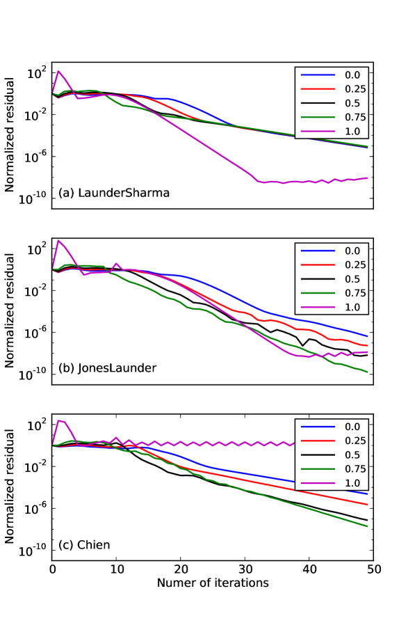
Figure 5: Plots of convergence history for a turbulent channel flow computed with NSCoupled. The different lines represent the choice of weight $e_{d}$ as indicated in the legend. The norms of the $u$ residuals (vertical axes) are plotted against the number of iterations (horizontal axes). In (a)-(c) we plot the results of using the LowReynolds_-Coupled solver with the LaunderSharma, JonesLaunder and Chien models, respectively.

6.2 Channel flow with and adverse pressure gradient

We now consider a channel that has a bump on the lower wall, thereby inducing an adverse pressure gradient that leads to separation on the decelerating side. The bump geometry is described by Marquillie et al. ³⁹, who performed Direct Numerical Simulations of the flow. The bump has also been studied experimentally at higher Reynolds numbers ³⁰, ⁴.

Adverse pressure gradient flows are notoriously difficult to model with simple RANS models. One particular reason for this is that regular wall function approaches do not work well, since the velocity profile near the wall will be far from the idealized log-law (see Figure 4.4 in Durbin and Pettersson Reif ¹⁸). Here we will employ the original four-equation V2F model of Durbin ¹⁷ (see Fig. 4) that does not employ wall functions, but involves special boundary condition-like terms. For numerical stability, these boundary conditions must be applied in a coupled and implicit manner, which is hard (if not impossible) to do with most commercial CFD software. We solve for the system composition [[’k’, ’e’], [’v2’, ’f’]], where the scalar $v^{2}$ resembles a wall normal stress and $f$ is a pressure redistribution parameter. The NS solver is the same as in the previous example.

For this example, homogeneous Dirichlet boundary conditions are applied to $u$, $k$ and $v^{2}$ on walls. Prescribed profiles for $k,\epsilon,v^{2}$ and $f$ on the inlet, obtained from an independent solution of a plain channel are used. The outlet uses a pseudo-traction-free condition ($\nabla{\mbox{\boldmath$u$}}\cdot n-pn=0$) and zero normal derivative for all other turbulence quantities. The “boundary conditions” used for $\epsilon$ and $f$ on walls are

$$\epsilon=\frac{2\nu k}{y^{2}}\text{ and }f=\frac{20\nu^{2}v^{2}}{y^{4}\epsilon},$$ (43)

respectively, where $y$ is the wall normal distance. This “boundary condition” cannot be set directly on the wall, because $y$ will be zero. However, $k/y$ approaches the wall as $O(1)$, and can be evaluated on the degrees of freedom close to the walls. In practice we set this boundary condition implicitly for $\epsilon$ and $f$ by manipulating the rows of the coefficient matrix that represent the degrees of freedom of elements in contact with a wall. The “boundary value” is computed for the degrees of freedom furthest from the wall for elements that are in contact with the wall. Within these elements, the fields are kept constant. The distance to the nearest wall $y$ is computed through a stabilized Eikonal equation, implemented as

    F = sqrt(inner(grad(y), grad(y)))*v*dx - f*v*dx \           + eps*inner(grad(y), grad(v))*dx,where f=Constant(1) and eps=Constant(0.01). The same FunctionSpace as for the turbulence parameters is used and the only assigned boundary conditions for $y$ are homogeneous Dirichlet on walls. The stabilized Eikonal equation is solved in just a few iterations using a Newton method.

We create a solver similar to solve_nonlinear where it is iterated between solving the NS-equations and the turbulence equations. Derived quantities are also updated between each subsystem’s solve. The flow field is initialized using the channel solution and the flow converges in about 50 iterations. Figure 6 shows the velocity and streamfunction (a), turbulent kinetic energy (b), and rate of energy dissipation (c) in the near vicinity of the bump. The streamfunction reveals that the flow separates on the decelerating side of the bump, in good agreement with direct numerical simulations of the same flow ³⁹. The streamfunction shown in Figure 6(a) has been computed in FEniCS through solving the Poisson equation $\nabla^{2}\psi=-\nabla\times{\mbox{\boldmath$u$}}$, which is implemented as

    q   = TestFunction(V)    psi = TrialFunction(V)    n = FacetNormal(mesh)    F = inner(grad(q), grad(psi))*dx \        - inner(q, (u[1].dx(0) - u[0].dx(1)))*dx \        + q*(n[1]*u[0] - n[0]*u[1])*ds.Here the boundary condition on the derivatives of $\psi$ (using $\nabla\times\psi={\mbox{\boldmath$u$}}$) is set weakly and it is noteworthy that this simple implementation applies for any 2 dimensional problem with any boundary. This would also be difficult to do in most CFD software.

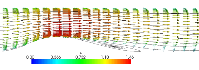
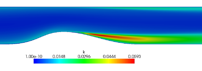
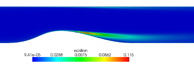
Figure 6: Computed quantities for flow past a bump using the $v^{2}-f$ model: (a) velocity vectors and streamfunction; (b) turbulent kinetic energy contours [m²/s²]; and (c) rate of energy dissipation [m²/s³].

7 Comments on computational efficiency

A key result from Section 5.3 is the convenient specification of the equations which define numerical schemes and how this specialized code is coupled with general code for handling an arbitrary system of PDEs. The user can freely choose between segregated and coupled formulations, as well as Picard-type or Newton iterations. A natural question is how this convenience and flexibility affects the computational efficiency.

Scripted programming languages inevitably involve an overhead cost that is greater than that for compiled languages. To reconcile this, FEniCS programs generate C++ code such that the solver carries out almost all computations in C++ (although this is transparent to the user, as outlined in Section 2.3). Furthermore, representations of finite element matrices and vectors can generated by a form compiler that are not tractable by hand ²⁶, and a range of domain-specific automated optimizations are applied to reduce the number of floating point operations ²⁵, ⁴². Therefore, we expect our FEniCS-based RANS solvers to have a computational efficiency superior to traditional, hand-written finite element solvers in C++. Comparisons with a state-of-the-art unstructured finite volume code CDP from Stanford for a test case show that an optimized version of our FEniCS-based NS solver is only approximately two times slower for some laminar flow cases. This is despite scope remaining for further optimizations of the FEniCS libraries and the extra flexibility offered by the finite element framework.

The Python overhead of turbulence solvers is mostly due to callbacks to Python from C++ for defining boundaries and initial conditions. The latter are computed only once per simulation, while boundary information is needed every time a linear system is computed. FEniCS has constructs for avoiding callbacks to Python by using just-in-time compilation, thereby eliminating the potential Python overhead.

8 Concluding remarks

We have presented a novel software framework for RANS modeling of turbulent flow. The framework targets researchers in computational turbulence who want full flexibility with respect to composing PDE models, coupling equations, linearizing equations and constructing iterative strategies for solving the nonlinear equations arising in RANS models.

The use of Python and FEniCS to realize the framework yields compact, high-level code, which in the authors’ opinions provides greater readability, flexibility and simplicity than what can be achieved with C++ or Fortran 2003. Throughout the text we have commented upon object-oriented designs via class hierarchies versus generative programming via stand-alone functions. It is the authors’ experiences that Python leads to a design more biased toward the generative style than does C++, perhaps because the generative style becomes so obvious in a language with dynamic typing. Although subclassing is a natural choice for users to provide new implementations, we have emphasized stand-alone functions as simpler and more flexible. Classes and dictionaries are used extensively in the code, but a disadvantage with Python, at least when implementing mathematical formulae, is the self prefix and other disturbing syntax. This disadvantage is overcome partly by a clever use of namespaces, as well as through the semi-automatic introduction of local variables.

Our computational examples illustrate two tasks that are easy to perform in the suggested framework, but usually hard to accomplish in other types of CFD software, namely an investigation of various linearizations in a family of turbulence models, and implementation of the promising $v^{2}$-$f$ model with different degree of implicitness.

Many more features than shown in this work can be added to the framework. For example, in FEniCS discontinuous Galerkin methods pose no difficulty for the programmer. FEniCS support for error control and adaptivity is also a promising topic to include and explore, especially since optimal mesh design is a major challenge in CFD. Unsteady RANS models with time dependency constitute an obvious extension, which essentially consists in adding suitable finite difference schemes for the time derivatives and a time loop in the code. The flexibility offered by FEniCS and the design of the RANS solvers makes the addition of new functionality straightforward.

We believe that our combination of mathematical formulations and specific code for the complicated class of PDE models addressed in this work demonstrate the power of Python and FEniCS as an expressive and human/computer-efficient software framework. Readers may use our implementation ideas in a wide range of science and engineering disciplines.

References

- Alnæs and Mardal [2010] M.S. Alnæs, K.A. Mardal, On the efficiency of symbolic computations combined with code generation for finite element methods, ACM Trans. Math. Software 37 (2010).
- Bangerth et al. [2007] W. Bangerth, R. Hartmann, G. Kanschat, deal.II – A general-purpose object-oriented finite element library, ACM Trans. Math. Software 33 (2007).
- Benim [2005] A.C. Benim, Finite element analysis of confined turbulent swirling flows, Int. J. Num. Methods in Fluids 11 (2005) 697–717.
- Bernard et al. [2003] A. Bernard, J.M. Foucaut, P. Dupont, M. Stanislas, Decelerating boundary layer: a new scaling and mixing length model, AIAA Journal 41 (2003) 248–255.
- Brenner and Scott [2008] S.C. Brenner, L.R. Scott, The Mathematical Theory of Finite Element Methods, volume 15 of Texts in Applied Mathematics, Springer, New York, third edition, 2008.
- Brown et al. [1997] D.L. Brown, W.D. Henshaw, D.J. Quinlan, Overture: An object oriented framework for solving partial differential equations, in: Y. Ishikawa, R.R. Oldehoeft, J.V.W. Reynders, M. Tholburn (Eds.), Scientific Computing in Object-Oriented Parallel Environments, Lecture Notes in Computer Science, Springer, 1997.
- Cactus [2011] Cactus, Software package, 2011. http://www.cactuscode.org/.
- cbc.rans [2011] cbc.rans, Software package, 2011. https://launchpad.net/cbc.rans.
- cbc.solve [2011] cbc.solve, Software package, 2011. https://launchpad.net/cbc.solve.
- Chien [1982] K.Y. Chien, Prediction of channel and boundary layer flows with a low reynolds number model, AIAA Journal 20 (1982) 33–38.
- COMSOL Multiphysics [2011] COMSOL Multiphysics, Software package, 2011. http://www.comsol.com.
- deal.II [2011] deal.II, Software package, 2011. http://www.dealii.org.
- Diffpack [2011] Diffpack, Software package, 2011. http://www.diffpack.com.
- Donea and Huerta [2003] J. Donea, A. Huerta, Finite Element Methods for Flow Problems, Wiley, 2003.
- Dular and Geuzaine [2011] P. Dular, C. Geuzaine, GetDP: a General environment for the treatment of Discrete Problems, 2011. http://www.geuz.org/getdp/.
- DUNE [2011] DUNE, The distributed and unified numerics environment, 2011. http://www.dune-project.org/dune.html.
- Durbin [1991] P.A. Durbin, Near-wall turbulence closure modeling without damping functions, Theoret. Comp. Fluid Dyn. 3 (1991) 1–13.
- Durbin and Pettersson Reif [2001] P.A. Durbin, B.A. Pettersson Reif, Statistical Theory and Modeling for Turbulent Flows, John Wiley and Sons, Chichester, 2001.
- FEniCS [2011] FEniCS, Software package, 2011. http://www.fenics.org.
- GetFEM++ [2011] GetFEM++, Software package, 2011. http://home.gna.org/getfem/.
- Ilinca et al. [2005] F. Ilinca, D. Pelletier, A. Garon, An adaptive finite element method for a two-equation turbulence model in wall-bounded flows, Int. J. Num. Methods in Fluids 24 (2005) 101–120.
- Jones and Launder [1972] W.P. Jones, B.E. Launder, The prediction of laminarization with a two-equation model of turbulence, Int. J. Heat Mass Transfer 15 (1972) 301–314.
- Joppich and Kürschner [2006] W. Joppich, M. Kürschner, MpCCI a tool for the simulation of coupled applications, Concurr. Comput.: Pract. Exper. 18 (2006) 183–192.
- Kassinos et al. [2000] S.C. Kassinos, C.A. Langer, S.L. Haire, W.C. Reynolds, Structure-based turbulence modeling for wall-bounded flows, Int. J. Heat and Fluid Flow 21 (2000) 599–605.
- Kirby et al. [2005] R.C. Kirby, M.G. Knepley, A. Logg, L.R. Scott, Optimizing the evaluation of finite element matrices, SIAM J. Sci. Comput. 27 (2005) 741–758.
- Kirby and Logg [2006] R.C. Kirby, A. Logg, A compiler for variational forms, ACM Trans. Math. Software 32 (2006) 417–444.
- Kirby and Logg [2007] R.C. Kirby, A. Logg, Efficient compilation of a class of variational forms, ACM Trans. Math. Software 33 (2007).
- Kirby and Logg [2008] R.C. Kirby, A. Logg, Benchmarking domain-specific compiler optimizations for variational forms, ACM Trans. Math. Software 35 (2008) 1–18.
- Kirby et al. [2006] R.C. Kirby, A. Logg, L.R. Scott, A.R. Terrel, Topological optimization of the evaluation of finite element matrices, SIAM J. Sci. Comput. 28 (2006) 224–240.
- Kostas et al. [2005] D. Kostas, J.M. Foucaut, M. Stanislas., Application of double SPIV on the near wall turbulence structure of an adverse pressure gradient turbulent boundary layer, in: 6th International Symposium on Particle Image Velocimetry, pp. 21–41.
- Langtangen [2003] H.P. Langtangen, Computational Partial Differential Equations - Numerical Methods and Diffpack Programming, Texts in Computational Science and Engineering, Springer, second edition, 2003.
- Langtangen et al. [2002] H.P. Langtangen, K.A. Mardal, R. Winther, Numerical methods for incompressible viscous flow, Adv. Water Res. 25 (2002) 1125–1146.
- Larson et al. [2005] J. Larson, R. Jacob, E. Ong, The model coupling toolkit: A new Fortran 90 toolkit for building multiphysics parallel coupled models, International Journal of High Performance Computing Applications 19 (2005) 277–292.
- Launder and Sharma [1974] B.E. Launder, B.I. Sharma, Application of the energy-dissipation model of turbulence to the calculation of flow near a spinning disc, Letters in Heat and Mass Transfer 1 (1974) 131–138.
- Logg [2007] A. Logg, Automating the finite element method, Arch. Comput. Methods Eng. 14 (2007) 93–138.
- Logg et al. [2011] A. Logg, K.A. Mardal, G.N. Wells (Eds.), Automated Scientitic Computing, Lecture Notes in Computational Science and Engineering, Springer, 2011. To appear, https://launchpad.net/fenics-book.
- Logg and Wells [2010] A. Logg, G.N. Wells, DOLFIN: Automated finite element computing, ACM Trans. Math. Software 37 (2010) 20:1–20:28.
- Lübon et al. [2009] C. Lübon, M. Kessler, S. Wagner, A parallel CFD solver using the discontinuous Galerkin approach, in: S. Wagner, M. Steinmetz, A. Bode, M. Brehm (Eds.), High Performance Computing in Science and Engineering, Springer, 2009.
- Marquillie et al. [2008] M. Marquillie, J.P. Laval, D. Rostislav, Direct numerical simulation of a separated channel flow with a smooth profile, J. Turbul. 9 (2008).
- Munthe and Langtangen [2000] O. Munthe, H.P. Langtangen, Finite elements and object-oriented implementation techniques in computational fluid dynamics, Comput. Methods Appl. Mech. Engrg. 190 (2000) 865–888.
- Ølgaard et al. [2008] K.B. Ølgaard, A. Logg, G.N. Wells, Automated code generation for discontinuous Galerkin methods, SIAM J. Sci. Comput. 31 (2008) 849–864.
- Ølgaard and Wells [2010] K.B. Ølgaard, G.N. Wells, Optimisations for quadrature representations of finite element tensors through automated code generation, ACM Trans. Math. Software 37 (2010) 8:1–8:23.
- OpenFOAM [2011] OpenFOAM, The open source CFD toolbox, 2011. http://www.openfoam.com.
- Overture [2011] Overture, Software package, 2011. https://computation.llnl.gov/casc/Overture.
- Peskin and Hardin [1996] A.P. Peskin, G.R. Hardin, An object-oriented approach to general purpose fluid dynamics software, Comput. Chem. Eng. 20 (1996) 1043–1058.
- Pope [2000] S.B. Pope, Turbulent flows, Cambridge University Press, 2000.
- Proteus [2011] Proteus, Software package, 2011. https://adh.usace.army.mil/proteus/.
- rheagen [2011] rheagen, Software package, 2011. https://launchpad.net/rheagen.
- Rognes et al. [2009] M. Rognes, R.C. Kirby, A. Logg, Efficient assembly of and conforming finite elements, SIAM J. Sci. Comput. 36 (2009) 4130–4151.
- Rouson et al. [2010] D.W.I. Rouson, H. Adalsteinsson, J. Xia, Design patterns for multiphysics modeling in Fortran 2003 and C++, ACM Trans. Math. Software 37 (2010).
- SAMRAI [2011] SAMRAI, Software package, 2011. https://computation.llnl.gov/casc/SAMRAI.
- Smith [2005] R.M. Smith, A practical method of two-equation turbulence modelling using finite elements, Int. J. Num. Methods in Fluids 4 (2005) 321–336.
- Spalart and Allmaras [1992] P.R. Spalart, S.R. Allmaras, A one-equation turbulence model for aerodynamic flows, AIAA Journal (1992) 92–439.
- Stewart and Edwards [2004] J.R. Stewart, H.C. Edwards, A framework approach for developing parallel adaptive multiphysics applications, Finite Elem. Anal. Des. 40 (2004) 1599–1617.
- Wells [2011] G.N. Wells, Multiphase flow through porous media, in: A. Logg, K.A. Mardal, G.N. Wells (Eds.), Automated Scientific Computing, Springer, 2011. To appear, https://launchpad.net/fenics-book.
- Wilcox [1988] D. Wilcox, Re-assessment of the scale-determining equation for advanced turbulence models, AIAA Journal 26 (1988) 1414–1421.
- www:fenics-apps [2011] www:fenics-apps, Software package, 2011. https://launchpad.net/fenics-group.