Fundamental Limits of Infinite Constellations in MIMO Fading Channels

Abstract

The fundamental and natural connection between the infinite constellation (IC) dimension and the best diversity order it can achieve is investigated in this paper. In the first part of this work we develop an upper bound on the diversity order of IC’s for any dimension and any number of transmit and receive antennas. By choosing the right dimensions, we prove in the second part of this work that IC’s in general and lattices in particular can achieve the optimal diversity-multiplexing tradeoff of finite constellations. This work gives a framework for designing lattices for multiple-antenna channels using lattice decoding.

I Introduction

The use of multiple antennas in wireless communication has certain inherent advantages. On one hand, using multiple antennas in fading channels allows to increase the transmitted signal reliability, i.e. diversity. For instance, diversity can be attained by transmitting the same information on different paths between transmitting-receiving antenna pairs with i.i.d Rayleigh fading distribution. The number of independent paths used is the diversity order of the transmitted scheme. On the other hand, the use of multiple antennas increases the number of degrees of freedom available by the channel. In [1],[2] the ergodic channel capacity was obtained for multiple-input multiple-output (MIMO) systems with $M$ transmit and $N$ receive antennas, where the paths have i.i.d Rayleigh fading distribution. It was shown that for large signal to noise ratios ($\mathsf{SNR}$), the capacity behaves as $C(\mathsf{SNR})\approx\min(M,N)\log(\mathsf{SNR})$. The multiplexing gain is the number of degrees of freedom utilized by the transmitted scheme.

For the quasi-static Rayleigh flat-fading channel, Zheng and Tse [3] characterized the dependence between the diversity order and the multiplexing gain, by deriving the optimal tradeoff between diversity and multiplexing, i.e. for each multiplexing gain the maximal diversity order was found. They showed that the optimal diversity-multiplexing tradeoff (DMT) can be attained by ensemble of i.i.d Gaussian codes, given that the block length is greater or equal to $N+M-1$. For this case, the tradeoff curve takes the form of the piecewise linear function that connects the points $(N-l)(M-l)$, $l=0,1,\dots,\min(M,N)$.

Space-time codes are coding schemes designed for MIMO systems e.g. see [4],[5] [6] and references therein. The design of space-time codes in these works pursue various goals such as maximizing the diversity order, maximizing the multiplexing gain, or achieving the optimal DMT. El Gamal et al [7] were the first to show that lattice coding and decoding achieve the optimal DMT. They presented lattice space-time (LAST) codes. These space time codes are subsets of an infinite lattice, where the lattice dimensionality equals to the number of degrees of freedom available by the channel, i.e. $\min(M,N)$, multiplied by the number of channel uses. By using a random ensemble of nested lattices, common randomness, minimum mean square error (MMSE) estimation followed by lattice decoding and modulo lattice operation, they showed that LAST codes can achieve the optimal DMT. It is worth mentioning that the MMSE estimation and the modulo operation take in a certain sense into account the finite code book.

There has been an extensive research on explicit coding schemes, based on lattices, which are DMT optimal. Such an explicit coding schemes that attain the optimal DMT for any number of transmit and receive antennas were presented in [6]. In addition it was shown in [6] that $M$ channel uses are sufficient to obtain the optimal DMT. Another step towards finding explicit space-time coding schemes that attain the optimal DMT with low computational complexity was made by Jalden and Elia [8]. They considered explicit coding schemes based on the intersection between an underlying lattice and a shaping region. They showed that for the cases where these coding schemes attain the optimal DMT using maximum-likelihood (ML) decoding, they also attain it when using MMSE estimation in the receiver, followed by lattice decoding. The MMSE estimation relies on the power constraint, i.e. the shaping region boundaries. In addition, it was shown in [8] that by applying lattice reduction methods, the optimal DMT is attained when using suboptimal linear lattice decoders that require linear complexity as a function of the rate. This result applies to wide range of explicit space-time codes such as golden-codes [9], perfect space-time codes [10] and in general cyclic division algebra based space-time codes [6], and as this codes are approximately universal [11] it also applies to every statistical characterization of the fading channel. Note that these schemes take into consideration the finiteness of the codebook in the decoder. In our work we refer to regular lattice decoding as decoding over the infinite lattice without taking into consideration the finiteness of the codebook.

The work in [7] also includes for the case $N\geq M$ a lower bound on the diversity order of LAST codes shaped into a sphere when regular lattice decoder is employed in the receiver. For sufficiently large block length it is shown that $d(r)\geq(N-M+1)(M-r)$ where $r$ is the multiplexing gain and the lattice dimension per channel use is $M$. Taherzadeh and Khandani showed in [12] that this is also an upper bound on the diversity order of any LAST code shaped into a sphere and decoded with regular lattice decoding. These results show that LAST codes together with regular lattice decoding are suboptimal compared to the optimal DMT of power constrained constellations.

Infinite constellations (IC’s) are structures in the Euclidean space that have no power constraint. In [13], Poltyrev analyzed the performance of IC’s over the additive white Gaussian noise (AWGN) channel. In this work we first extend the definitions of diversity order and multiplexing gain to the case where there is no power constraint. We also introduce a new term: the average number of dimensions per channel use, which is essentially the IC dimension divided by the number of channel uses. Then we extend the methods used in [13] in order to derive an upper bound on the diversity of any IC with certain average number of dimensions per channel use, as a function of the multiplexing gain. It turns out that for a given number of dimensions per channel use the diversity is a straight line as a function of the multiplexing gain, that depends on the number of transmit and receive antennas. This analysis holds for $any$ $M$ and $N$, and also applies for lattices with regular lattice decoding. We also find the average number of dimensions per channel use for which the upper bounds coincide with the optimal DMT of finite constellations. Finally, we show that each segment in the optimal DMT is attained by a sequence of lattices with a corresponding average number of dimensions per channel use, when using regular lattice decoder, i.e. for each point in the DMT of [3] there exists a lattice sequence of certain dimension that achieves it with regular lattice decoding. Hence, this work characterizes the best DMT IC’s may attain for any average number of dimensions per channel use, and also proves that lattices can achieve the optimal DMT when regular lattice decoder is employed in the receiver, by adapting their dimensionality. It is important to note that when the IC is a lattice, we show that the multiplexing gain of infinite lattices and finite constellations coincide.

This work gives a framework for designing lattices for multiple-antenna channels using regular lattice decoding. It also shows the fundamental and natural connection between the IC dimension and its optimal diversity order. For instance, it is shown that for the case $M=N=2$, the maximal diversity order of $4$ can be achieved (with regular lattice decoding) by a lattice that has at most $\frac{4}{3}$ average number of dimensions per channel use. On the other hand the Alamouti scheme [14], that also has maximal diversity order of $4$, utilizes only a single dimension per channel use in this set up. Hence, there is still a room to improve by a $\frac{1}{3}$ of a dimension per channel use. In addition, while in [7], [8], the MMSE estimation improves the channel in such a manner that enables the lattice decoder to attain the optimal DMT, this work shows that when considering regular lattice decoding, reducing the lattice dimensionality takes the role of MMSE estimation in the sense of improving the channel such that the optimal DMT is obtained. Finally, the analysis in this work gives another geometrical interpretation to the optimal DMT.

The outline of the paper is as follows. In section II basic definitions for the fading channel and IC’s are given. Section III presents for each channel realization a lower bound on the average decoding error probability of any IC, and an upper bound on the DMT of any IC. An upper bound on the error probability of ensemble of IC’s for each channel realization, a transmission scheme that attains the optimal DMT, and some averaging arguments on how the optimal DMT is attained by IC’s, are all presented in section IV. Discussion on the results, that addresses the difference between lattice constellations and full dimension lattice based finite constellations, followed by a geometrical interpretation to the optimal DMT, and a discussion on the relation between the multiplexing gains of an IC and a finite constellation, is presented in section V. This discussion presents an intuitive interpretation to our results and relies mainly on the basic definitions given in section II.

II Basic Definitions

We refer to the countable set $S=\{s_{1},s_{2},\dots\}$ in $\mathbb{C}^{n}$ as infinite constellation (IC). Let $\mathrm{cube}_{l}(a)\subset\mathbb{C}^{n}$ be a (probably rotated) $l$-complex dimensional cube ($l\leq n$) with edge of length $a$ centered around zero. An IC $S_{l}$ is $l$-complex dimensional if there exists rotated $l$-complex dimensional cube $\mathrm{cube}_{l}(a)$ such that $S_{l}\subset\lim_{a\to\infty}\mathrm{cube}_{l}(a)$ and l is minimal. $M(S_{l},a)=|S_{l}\bigcap\mathrm{cube}_{l}(a)|$ is the number of points of the IC $S_{l}$ inside $\mathrm{cube}_{l}(a)$. In [13], the $n$-complex dimensional IC density for the AWGN channel was defined as the upper limit (the limit supremum) of the ratio $\gamma_{\mathrm{G}}=\limsup_{a\to\infty}\frac{M(S,a)}{a^{2n}}$ and the volume to noise ratio (VNR) was given as $\mu_{\mathrm{G}}=\frac{\gamma_{\mathrm{G}}^{-\frac{1}{n}}}{2\pi e\sigma^{2}}$.

The Voronoi region of a point $x\in S_{l}$, denoted as $V(x)$, is the set of points in $\lim_{a\to\infty}\mathrm{cube}_{l}(a)$ closer to $x$ than to any other point in the IC. The effective radius of the point $x\in S_{l}$, denoted as $r_{\mathrm{eff}}(x)$, is the radius of the $l$-complex dimensional ball that has the same volume as the Voronoi region, i.e. $r_{\mathrm{eff}}(x)$ satisfies

$$|V(x)|=\frac{\pi^{l}r_{\mathrm{eff}}^{2\cdot l}(x)}{\Gamma(l+1)}.$$ (1)

A complex lattice $\Lambda$ is an IC that constitutes a discrete set in $\mathbb{C}^{n}$, closed under addition. The Voronoi regions of all lattice points are identical and satisfy

$$|V\left(\underline{x}\right)|=\gamma_{G}^{-1}\quad\forall\underline{x}\in\Lambda.$$ (2)

Hence, for large dimension the VNR of a lattice, $\mu_{G}$, approaches the ratio $\frac{r_{\mathrm{eff}}^{2}}{\sigma^{2}}$ where $r_{\mathrm{eff}}$ is the lattice effective radius. Regular lattice decoder finds the closest lattice point to an observation $\underline{y}\in\mathbb{C}^{n}$, i.e. regular lattice decoder finds the solution to the optimization problem

$$\arg\min_{\underline{x}\in\Lambda}\lVert\underline{y}-\underline{x}\rVert.$$ (3)

Note that these definitions can be also extended in a straight forward manner to an IC that constitutes a real lattice in $\mathbb{R}^{2n}$. For instance when the first $n$ entries of each lattice point are transmitted on the real part of the IC, and the second $n$ entries of each lattice point are transmitted on the imaginary part of the IC.

We consider a quasi static flat-fading channel with $M$ transmit and $N$ receive antennas. We assume for this MIMO channel perfect channel knowledge at the receiver and no channel knowledge at the transmitter. The channel model is as follows:

$$\underline{y}_{t}=H\cdot\underline{x}_{t}+\rho^{-\frac{1}{2}}\underline{n}_{t}\qquad t=1,\dots,T$$ (4)

where $\underline{x}_{t}$, $t=1,\dots,T$ is the transmitted signal, $\underline{n}_{t}\sim CN(\underline{0},\frac{2}{2\pi e}I_{N})$ is the additive noise where $CN$ denotes complex-normal, $I_{N}$ is the $N$-dimensional unit matrix, and $\underline{y}_{t}\in\mathbb{C}^{N}$. $H$ is the fading matrix with $N$ rows and $M$ columns where $h_{i,j}\sim CN(0,1)$, $1\leq i\leq N$, $1\leq j\leq M$, and $\rho^{-\frac{1}{2}}$ is a scalar that multiplies each element of $\underline{n}_{t}$, where $\rho$ plays the role of average $\mathsf{SNR}$ in the receive antenna for power constrained constellations that satisfy $\frac{1}{T}\sum_{t=1}^{T}E\{\lVert\underline{x}_{t}\rVert^{2}\}\leq\frac{2}{2\pi e}$.

We also define the extended vector $\underline{x}=\{\underline{x}_{1}^{\dagger},\dots,\underline{x}_{T}^{\dagger}\}^{\dagger}$. Suppose $\underline{x}\in S_{l}\subset\mathbb{C}^{MT}$, where $S_{l}$ is an IC with density $\gamma_{tr}=\limsup_{a\to\infty}\frac{M(S_{l},a)}{a^{2\cdot l}}$ $\big{(}a^{2\cdot l}$ is the volume of $cube_{l}(a)\big{)}$. By defining $H_{ex}$ as an $NT\times MT$ block diagonal matrix, where each block on the diagonal equals $H$, $\underline{n}_{\mathrm{ex}}=\rho^{-\frac{1}{2}}\cdot\{\underline{n}_{1}^{\dagger},\dots,\underline{n}_{T}^{\dagger}\}^{\dagger}\in\mathbb{C}^{NT}$ and $\underline{y}_{\mathrm{ex}}\in\mathbb{C}^{NT}$ we can rewrite the channel model in (4) as

$$\underline{y}_{\mathrm{ex}}=H_{\mathrm{ex}}\cdot\underline{x}+\underline{n}_{\mathrm{ex}}.$$ (5)

In the sequel we use $L$ to denote $min(M,N)$. We define as $\sqrt{\lambda}_{i}$, $1\leq i\leq L$ the real valued, non-negative singular values of $H$. We assume $\sqrt{\lambda}_{L}\geq\dots\geq\sqrt{\lambda}_{1}>0$. Our analysis is done for large values of $\rho$ (large VNR at the transmitter). We state that $f(\rho)\dot{\geq}g(\rho)$ when $\lim_{\rho\to\infty}-\frac{\ln\left(f\left(\rho\right)\right)}{\ln(\rho)}\leq-\frac{\ln\left(g\left(\rho\right)\right)}{\ln(\rho)}$, and also define $\dot{\leq}$, $\dot{=}$ in a similar manner by substituting $\leq$ with $\geq$, $=$ respectively.

We now turn to the IC definitions in the transmitter. We define the average number of dimensions per channel use as the IC dimension divided by the number of channel uses. We denote the average number of dimensions per channel use by $K$. Let us consider a $KT$-complex dimensional sequence of IC’s $S_{KT}(\rho)$, where $K\leq L$, and $T$ is the number of channel uses. First we define $\gamma_{tr}=\rho^{rT}$ as the density of $S_{KT}(\rho)$ in the transmitter. The IC multiplexing gain is defined as

$$MG(r)=\lim_{\rho\to\infty}\frac{1}{T}\log_{\rho}(\gamma_{\mathrm{tr}}+1)=\lim_{\rho\to\infty}\frac{1}{T}\log_{\rho}(\rho^{rT}+1).$$ (6)

Note that $MG(r)=max(0,r)$, i.e. for $0\leq r\leq K$ the multiplexing gain is $r$. Roughly speaking, $\gamma_{tr}=\rho^{rT}$ gives us the number of points of $S_{KT}(\rho)$ within the $KT$-complex dimensional region $cube_{KT}(1)$. In order to get the multiplexing gain, we normalize the exponent of the number of points within $cube_{KT}(1)$, $rT$, by the number of channel uses - $T$. Note that the IC multiplexing gain, $r$, can be directly translated to finite constellation multiplexing gain $r$ by considering the IC points within a shaping region. For more details see V-C. The VNR in the transmitter is

$$\mu_{\mathrm{tr}}=\frac{\gamma_{\mathrm{tr}}^{-\frac{1}{KT}}}{2\pi e\sigma^{2}}=\rho^{1-\frac{r}{K}}$$ (7)

where $\sigma^{2}=\frac{\rho^{-1}}{2\pi e}$ is each dimension noise variance. Now we can understand the role of the multiplexing gain for IC’s. The AWGN variance decreases as $\rho^{-1}$, where the IC density increases as $\rho^{rT}$. When $r=0$ we get constant IC density as a function of $\rho$, where the noise variance decreases, i.e. we get the best error exponent. In this case the number of points within $cube_{KT}(1)$ remains constant as a function of $\rho$. On the other hand, when $r=K$, we get VNR $\mu_{tr}=1$, and from [13] we know that it inflicts average error probability that is bounded away from zero. In this case, the increase in the number of IC points within $cube_{KT}(1)$ occurs at maximal rate.

Now we turn to the IC definitions in the receiver. First we define the set $H_{ex}\cdot cube_{KT}(a)$ as the multiplication of each point in $cube_{KT}(a)$ with the matrix $H_{ex}$. In a similar manner $S_{KT}^{{}^{\prime}}=H_{ex}\cdot S_{KT}$. The set $H_{ex}\cdot cube_{KT}(a)$ is almost surely $KT$-complex dimensional (where $K\leq L$) and in this case $M(S_{KT},a)=|S_{KT}\bigcap\mathrm{cube}_{KT}(a)|=|S_{KT}^{{}^{\prime}}\bigcap(H_{ex}\cdot\mathrm{cube}_{KT}(a))|$. We define the receiver density as

$$\gamma_{\mathrm{rc}}=\limsup_{a\to\infty}\frac{M(S_{KT},a)}{\mathbf{Vol}(H_{ex\cdot}\mathrm{cube}_{KT}(a))}$$

i.e., the upper limit of the ratio of the number of IC points in $H_{ex\cdot}\mathrm{cube}_{KT}(a)$, and the volume of $H_{ex\cdot}\mathrm{cube}_{KT}(a)$. Based on the majorization property of a matrix singular values [15], we get that the volume of the set $H_{ex}\cdot cube_{KT}(a)$ is smaller than $a^{2KT}\cdot\lambda_{L}^{T}\dots\lambda_{L-B+1}^{T}\cdot\lambda_{L-B}^{\beta T}$, assuming $K=B+\beta$ where $B\in\mathbb{N}$ and $0<\beta\leq 1$, i.e. the volume is smaller than the multiplication of the $B+1$ strongest singular values, raised to the power of the maximal amount of channel uses each can take place in. Hence we get

$$\gamma_{\mathrm{rc}}\geq\rho^{rT}\lambda_{L}^{-T}\dots\lambda_{L-B+1}^{-T}\cdot\lambda_{L-B}^{-\beta T}$$ (8)

and the receiver VNR is

$$\mu_{\mathrm{rc}}\leq\rho^{1-\frac{r}{K}}\cdot\lambda_{L}^{\frac{1}{K}}\dots\lambda_{L-B+1}^{\frac{1}{K}}\cdot\lambda_{L-B}^{\frac{\beta}{K}}.$$ (9)

Note that for $N\geq M$ and $K=M$ we get $\gamma_{\mathrm{rc}}=\rho^{rT}\cdot\prod_{i=1}^{M}\lambda_{i}^{-T}$ and $\mu_{\mathrm{rc}}=\rho^{1-\frac{r}{M}}\cdot\prod_{i=1}^{M}\lambda_{i}^{\frac{1}{M}}$. The average decoding error probability over the IC points of $S_{KT}(\rho)$, for a certain channel realization $H$, is defined as

$$\overline{P_{e}}(H,\rho)=\limsup_{a\to\infty}\frac{\sum_{\underline{x}^{{}^{\prime}}\in S_{KT}^{{}^{\prime}}\bigcap(H_{ex}\cdot\mathrm{cube}_{KT}(a))}P_{e}(\underline{x}^{{}^{\prime}},H,\rho)}{M(S_{KT},a)}$$ (10)

where $P_{e}(\underline{x}^{{}^{\prime}},H,\rho)$ is the error probability associated with $\underline{x}^{{}^{\prime}}$. The average decoding error probability of $S_{KT}(\rho)$ over all channel realizations is $\overline{P_{e}}(\rho)=E_{H}\{\overline{P_{e}}(H,\rho)\}$. Hence the $diversity$ $order$ equals

$$d=-\lim_{\rho\to\infty}\log_{\rho}(\overline{P_{e}}(\rho))$$ (11)

III Upper Bound on the Diversity Order

In this section we derive an upper bound on the diversity order of any IC with average number of dimensions per channel use $K$ and any value of $T$, $M$ and $N$. In Theorem 1 we derive for each channel realization a lower bound on the error probability of any IC with $K$ average number of dimensions per channel use. In Theorem 2 we derive an upper bound on the DMT of any sequence of IC’s with $K$ average number of dimensions per channel use. Finally in Corollary 2 we show that by choosing the correct average number of dimensions per channel use, the upper bound coincides with the optimal DMT of finite constellations.

As in [3] and [7], we also define $\lambda_{i}=\rho^{-\alpha_{i}}$, $1\leq i\leq L$. When the entries of the channel matrix $H$ are all i.i.d with PDF $CN(0,1)$, the PDF of its singular values is of the form $\rho^{-\sum_{i=1}^{L}(|N-M|+2i-1)\alpha_{i}}$ for large $\rho$ [3], where following the definitions above $0\leq\alpha_{L}\leq\dots\leq\alpha_{1}$. By assigning in (8), (9) respectively, we can write

$$\gamma_{\mathrm{rc}}\geq\rho^{T(r+\sum_{i=0}^{B-1}\alpha_{L-i}+\beta\alpha_{L-B})}$$

and

$$\mu_{\mathrm{rc}}\leq\rho^{1-\frac{1}{K}(r+\sum_{i=0}^{B-1}\alpha_{L-i}+\beta\alpha_{L-B})}.$$

Theorem 1.

For any $KT$-complex dimensional IC $S_{KT}(\rho)$ with transmitter density $\gamma_{\mathrm{tr}}=\rho^{rT}$ and channel realization $\underline{\alpha}=(\alpha_{1},\dots,\alpha_{L})$, we have the following lower bound on the average decoding error probability for $0\leq r\leq K$

$$\overline{P_{e}}(H,\rho)>\frac{C(KT)}{4}e^{-\mu_{\mathrm{rc}}\cdot A(KT)+(KT-1)\ln(\mu_{\mathrm{rc}})}$$

where $A(KT)=e\cdot\Gamma(KT+1)^{\frac{1}{KT}}$ and $C(KT)=\frac{e^{KT-\frac{3}{2}}\Gamma(KT+1)^{\frac{KT-1}{KT}}}{2\cdot\Gamma(KT)}$.

Proof.

We divide the proof into two parts. In the first part we prove the result for lattices, that constitute a symmetric structure for which the Voronoi regions of different lattice points are identical. In the second part we prove the result for general IC’s with receiver density $\gamma_{rc}$. As the second part of the proof is somewhat more involved, we defer it to appendix A. Note that we could have used the tighter bounds of [17], but these bounds are not needed for DMT. Instead we derive coarser and more simplified upper bounds, which are sufficient for our purposes.

We begin by proving the result for lattices. Lattices constitute a discrete subgroup of the Euclidean space, with the ordinary vector addition operation. Consider a $KT$-complex dimensional lattice, $S^{{}^{\prime}}_{KT}(\rho)$, in the receiver with density $\gamma_{rc}$. The lattice points have identical Voronoi regions up to a translation. Hence, the volume of each Voronoi region equals

$$|V(x)|=\frac{1}{\gamma_{rc}}\quad\forall x\in S^{{}^{\prime}}_{KT}(\rho).$$

According to the definition of the effective radius in (1), we get that $r_{\mathrm{eff}}(x)=r_{\mathrm{eff}}(\gamma_{rc})=(\frac{\Gamma(KT+1)}{\gamma_{rc}\pi^{KT}})^{\frac{1}{2KT}}$, $\forall x\in S^{{}^{\prime}}_{KT}(\rho)$. Note that in lattices the maximum-likelihood (ML) decoding error probability is identical for all lattice points, i.e. the average and maximal error probabilities are identical. It has been proven in [13], [18] that the error probability of any lattice point in the receiver fulfils

$$P_{e}^{S^{{}^{\prime}}_{KT}}>Pr(\lVert\underline{\tilde{n}}_{\mathrm{ex}}\rVert\geq r_{\mathrm{eff}}(\gamma_{rc}))$$

where $P_{e}^{S^{{}^{\prime}}_{KT}}$ is the ML decoding error probability of any lattice point, and $\underline{\tilde{n}}_{\mathrm{ex}}$ is the effective noise in the $KT$-complex dimensional hyperplane where $S^{{}^{\prime}}_{KT}(\rho)$ resides. We find an explicit expression for the lower bound

$$\Pr\big{(}\lVert\underline{\tilde{n}}_{\mathrm{ex}}\rVert\geq r_{\mathrm{eff}}(\gamma_{\mathrm{rc}})\big{)}>\Pr\big{(}\lVert\underline{\tilde{n}}_{\mathrm{ex}}\rVert\geq r_{\mathrm{eff}}(\frac{\gamma_{\mathrm{rc}}}{2})\big{)}>\int_{r_{\mathrm{eff}}^{2}}^{r_{\mathrm{eff}}^{2}+\sigma^{2}}\frac{r^{KT-1}e^{-\frac{r}{2\sigma^{2}}}}{\sigma^{2KT}2^{KT}\Gamma(KT)}dr\geq\frac{r_{\mathrm{eff}}^{2KT-2}e^{-\frac{r_{\mathrm{eff}}^{2}}{2\sigma^{2}}}}{\sigma^{2KT-2}2^{KT}\Gamma(KT)\sqrt{e}}.$$ (12)

By assigning $r_{\mathrm{eff}}^{2}=(\frac{2\cdot\Gamma(KT+1)}{\gamma_{rc}\pi^{KT}})^{\frac{1}{KT}}$ we get

$$P_{e}^{S^{{}^{\prime}}_{KT}}>C(KT)\cdot e^{-\frac{\gamma_{\mathrm{rc}}^{-\frac{1}{KT}}}{2\pi e\sigma^{2}}A(KT)+(KT-1)\ln(\frac{\gamma_{\mathrm{rc}}^{-\frac{1}{KT}}}{2\pi e\sigma^{2}})}$$

and by assigning $\mu_{rc}=\frac{\gamma_{\mathrm{rc}}^{-\frac{1}{KT}}}{2\pi e\sigma^{2}}$ we get

$$P_{e}^{S^{{}^{\prime}}_{KT}}>\frac{C(KT)}{4}\cdot e^{-\mu_{rc}A(KT)+(KT-1)\ln(\mu_{rc})}.$$ (13)

Note that in (12) we lower bounded the error probability with $r_{\mathrm{eff}}(\frac{\gamma_{rc}}{2})$ instead of $r_{\mathrm{eff}}(\gamma_{rc})$, and also in (13) we multiplied by $\frac{1}{4}$, in order to be consistent with the general lower bound for IC’s shown in appendix A. For lattices we have $\overline{P_{e}}(H,\rho)=P_{e}^{S^{{}^{\prime}}_{KT}}$. Essentially what we have shown here is a scaled sphere packing bound. ∎

Next, we would like to use this lower bound to average over the channel realizations and get an upper bound on the diversity order.

Theorem 2.

The diversity order of any $KT$-complex dimensional sequence of IC’s $S_{KT}(\rho)$, with $K$ average number of dimensions per channel use, is upper bounded by

$$d_{KT}(r)\leq d^{\ast}_{K}(r)=M\cdot N(1-\frac{r}{K})$$

for $0<K\leq\frac{M\cdot N}{N+M-1}$, and

$$d_{KT}(r)\leq d^{\ast}_{K}(r)=(M-l)(N-l)\frac{K}{K-l}(1-\frac{r}{K})$$

for $\frac{(M-l+1)(N-l+1)}{N+M-1-2(l-1)}+l-1<K\leq\frac{(M-l)(N-l)}{N+M-1-2\cdot l}+l$ and $l=1,\dots,L-1$. In all of these cases $0\leq r\leq K$.

Proof.

For any IC with VNR $\mu_{rc}$, assigning $\mu_{rc}^{{}^{\prime}}>\mu_{rc}$ in the lower bound from Theorem 1 also gives a lower bound on the error probability

$$\overline{P_{e}}(H,\rho)>\frac{C(KT)}{4}e^{-\mu_{\mathrm{rc}}^{{}^{\prime}}\cdot A(KT)+(KT-1)\ln(\mu_{\mathrm{rc}}^{{}^{\prime}})}.$$

It results from the fact that inflating the IC into an IC with VNR $\mu_{rc}^{{}^{\prime}}$ must decrease the error probability, where

$$\frac{C(KT)}{4}e^{-\mu_{\mathrm{rc}}^{{}^{\prime}}\cdot A(KT)+(KT-1)\ln(\mu_{\mathrm{rc}}^{{}^{\prime}})}$$

is a lower bound on the error probability of any IC with VNR $\mu_{rc}^{{}^{\prime}}$. Hence, for the case $\mu_{rc}\leq 1$ we can lower bound the error probability by assigning 1 in the lower bound and get $\frac{C(KT)}{4}e^{-A(KT)}$, i.e. for $\mu_{rc}\leq 1$ the average decoding error probability is bounded away from 0 for any value of $\rho$. We can give the event $\mu_{rc}\leq 1$ the interpretation of an outage event.

We would like to set a lower bound for the error probability for each channel realization $\underline{\alpha}$, which we denote by $P_{e}^{LB}(\rho,\underline{\alpha})$. We know that $\mu_{\mathrm{rc}}\leq\rho^{1-\frac{1}{K}(r+\sum_{i=0}^{B-1}\alpha_{L-i}+\beta\alpha_{L-B})}$. For the case $\sum_{i=0}^{B-1}\alpha_{L-i}+\beta\alpha_{L-B}<K-r$, we take

$$P_{e}^{LB}(\rho,\underline{\alpha})=\frac{C(KT)}{4}e^{-L(\rho,\underline{\alpha})\cdot A(KT)+(KT-1)\ln(L(\rho,\underline{\alpha}))}$$

where $L(\rho,\underline{\alpha})=\rho^{1-\frac{1}{K}(r+\sum_{i=0}^{B-1}\alpha_{L-i}+\beta\alpha_{L-B})}>1$. For the case $\sum_{i=0}^{B-1}\alpha_{L-i}+\beta\alpha_{L-B}\geq K-r$ we get that $\mu_{rc}\leq 1$, and we take

$$P_{e}^{LB}(\rho,\underline{\alpha})=\frac{C(KT)}{4}e^{-A(KT)}.$$

In order to find an upper bound on the diversity order, we would like to average $P_{e}^{LB}(\rho,\underline{\alpha})$ over the channel realizations. In our analysis we consider large values of $\rho$, and so we calculate

$$\overline{P_{e}}(\rho)\dot{>}\int_{\underline{\alpha}\geq 0}P_{e}^{LB}(\rho,\underline{\alpha})\cdot\rho^{-\sum_{i=1}^{L}(|N-M|+2i-1)\alpha_{i}}d\underline{\alpha}$$ (14)

where $\underline{\alpha}\geq 0$ signifies the fact that $\alpha_{1}\geq\dots\geq\alpha_{L}\geq 0$. By defining $\mathcal{A}=\{\underline{\alpha}|\sum_{i=0}^{B-1}\alpha_{L-i}+\beta\alpha_{L-B}<K-r;\underline{\alpha}\geq 0\}$ and $\overline{\mathcal{A}}=\{\underline{\alpha}|\sum_{i=0}^{B-1}\alpha_{L-i}+\beta\alpha_{L-B}\geq K-r;\underline{\alpha}\geq 0\}$ we can split (14) into 2 terms

$$\overline{P_{e}}(\rho)\dot{>}\int_{\underline{\alpha}\in\mathcal{A}}P_{e}^{LB}(\rho,\underline{\alpha})\cdot\rho^{-\sum_{i=1}^{L}(|N-M|+2i-1)\alpha_{i}}d\underline{\alpha}+\int_{\underline{\alpha}\in\overline{\mathcal{A}}}P_{e}^{LB}(\rho,\underline{\alpha})\cdot\rho^{-\sum_{i=1}^{L}(|N-M|+2i-1)\alpha_{i}}d\underline{\alpha}.$$ (15)

Hence

$$\overline{P_{e}}(\rho)\dot{>}\int_{\underline{\alpha}\in\overline{\mathcal{A}}}P_{e}^{LB}(\rho,\underline{\alpha})\cdot\rho^{-\sum_{i=1}^{L}(|N-M|+2i-1)\alpha_{i}}d\underline{\alpha}.$$ (16)

In a similar manner to [3], [7], for very large $\rho$, we approximate the average value by finding the most dominant exponential term in the integral. For this we would like to find the minimal value of

$$\lim_{\rho\to\infty}-\log_{\rho}(P_{e}^{LB}(\rho,\underline{\alpha})\cdot\rho^{-\sum_{i=1}^{L}(|N-M|+2i-1)\alpha_{i}})$$

for the case $\underline{\alpha}\in\overline{\mathcal{A}}$. For $\underline{\alpha}\in\overline{\mathcal{A}}$, we get that $P_{e}^{LB}(\rho,\underline{\alpha})$ is bounded away from 0 for any value of $\rho$. Hence, in order to find the most dominant error event we would like to find $\min_{\underline{\alpha}}\sum_{i=1}^{L}(|N-M|+2i-1)\alpha_{i}$ given that $\underline{\alpha}\in\overline{\mathcal{A}}$. The minimal value is achieved at the boundary, i.e. for $\underline{\alpha}$ satisfying $\sum_{i=0}^{B-1}\alpha_{L-i}+\beta\alpha_{L-B}=K-r$, $\underline{\alpha}\geq 0$. Hence, for any $K\leq L$ we state that

$$d_{KT}(r)\leq\min_{\underline{\alpha}}\sum_{i=1}^{L}(|N-M|+2i-1)\alpha_{i},\qquad 0\leq r\leq K$$ (17)

where $\sum_{i=0}^{B-1}\alpha_{L-i}+\beta\alpha_{L-B}=K-r$ and $\alpha_{1}\geq\dots\geq\alpha_{L}\geq 0$. Basically this optimization problem is a linear programming problem whose solution is as follows. For $0<K\leq\frac{M\cdot N}{N+M-1}$ the solution is $\alpha_{i}=1-\frac{r}{K}$, $i=1,\dots,L$. For $\frac{(M-l+1)(N-l+1)}{N+M-1-2(l-1)}+l-1<K\leq\frac{(M-l)(N-l)}{N+M-1-2\cdot l}+l$ and $l=1,\dots,L-1$ the solution is $\alpha_{L}=\dots=\alpha_{L-l+1}=0$ and $\alpha_{L-l}=\dots=\alpha_{1}=\frac{K-r}{K-l}$. The desired upper is attained by substituting the optimal values of $\underline{\alpha}$ in (17). The detailed solution for the optimization problem is presented in appendix B. ∎

From Theorem 2 we get an upper bound on the diversity order by assuming transmission of the $KT$ complex dimensions over the $B+1$ strongest singular values. This assumption is equivalent to assuming beamforming which may improve the coding gain, but does not increase the diversity order. This assumption allows us to derive a lower bound on the average decoding error probability. However, we still get maximal diversity order of $MN$ in this case.

Let us consider as an illustrative example the case of $M=N=2$. In this case, for $0<K\leq\frac{4}{3}$ we get $d_{K}^{\ast}(r)=4(1-\frac{r}{K})$. For $\frac{4}{3}<K\leq 2$ we get $d_{k}^{\ast}(r)=\frac{K}{K-1}(1-\frac{r}{K})$. In both cases $0\leq r\leq K$. For this set up we have two singular values and so $\alpha_{1}\geq\alpha_{2}\geq 0$. The optimization problem is of the form $\min_{\underline{\alpha}\geq 0}\alpha_{1}+3\alpha_{2}$, where for $0<K\leq 1$ the constraint is $\beta\alpha_{2}=K-r$, and for $1<K\leq 2$ the constraint is $\alpha_{2}+\beta\alpha_{1}=K-r$. For the case $0<K<\frac{4}{3}$ the optimization problem solution is $\alpha_{1}=\alpha_{2}=1-\frac{r}{K}$, i.e. in this case the most dominant error event occurs when both singular values are very small. For the case $K=\frac{4}{3}$ the constraint is of the form $\alpha_{2}+\frac{\alpha_{1}}{3}=\frac{4}{3}-r$, and the optimization problem solution is achieved for both $\alpha_{1}=\alpha_{2}=1-\frac{3r}{4}$ and $\alpha_{2}=0$, $\alpha_{1}=4-3r$. For the case $\frac{4}{3}<K\leq 2$ the optimization problem solution is achieved for $\alpha_{2}=0$, $\alpha_{1}=\frac{K-r}{K-1}$, i.e. one strong singular value and another very weak singular value.

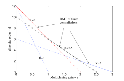
Figure 1: The diversity order as a linear function of the multiplexing gain $r$ for $M=4$, $N=3$ and $K=1$, $2$, $2.5$ and $3$.

Corollary 1.

For $0<K\leq\frac{M\cdot N}{N+M-1}$ we get $d^{\ast}_{K}(0)=MN$. For $\frac{(M-l+1)(N-l+1)}{N+M-1-2(l-1)}+l-1<K\leq\frac{(M-l)(N-l)}{N+M-1-2\cdot l}+l$, $l=1,\dots,L-1$ we get $d^{\ast}_{K}(l)=(M-l)(N-l)$.

Proof.

The proof is straight forward from $d_{K}^{\ast}(r)$ properties. ∎

From Corollary 1 we get that the range of $K$ can be divided into segments, where for each segment we have a set of straight lines, that are all equal at a certain integer point. Note that at these points, we get the same values as the optimal DMT for finite constellations.

Corollary 2.

In the range $l\leq r\leq l+1$, the maximal possible diversity order is achieved at dimension $K_{l}=\frac{(M-l)(N-l)}{N+M-1-2\cdot l}+l$ and equals

$$d^{\ast}_{K_{l}}(r)=(M-l)(N-l)\frac{K_{l}}{K_{l}-l}(1-\frac{r}{K_{l}})$$

$$=(M-l)(N-l)-(r-l)(N+M-2\cdot l-1)$$

where $l=0,\dots,L-1$. This expression equals to the optimal DMT of finite constellations in this range.

Proof.

The proof is straight forward from $d_{K}^{\ast}(r)$ properties. ∎

From Corollary 2 we can see that $d_{K_{l}}^{\ast}(l)=(M-l)(N-l)$ and $d_{K_{l}}^{\ast}(l+1)=(M-l-1)(N-l-1)$. We also know that $d_{K_{l}}^{\ast}(r)$ is a straight line. Also, the optimal DMT for finite constellations consists of a straight line in the range $l\leq r\leq l+1$, that equals $(N-l)(M-l)$ when $r=l$ and $(M-l-1)(N-l-1)$ when $r=l+1$. Hence, in the range $l\leq r\leq l+1$ for $K_{l}=\frac{(M-l)(N-l)}{N+M-1-2\cdot l}+l$, we get an upper bound that equals to the optimal DMT of finite constellations presented in [3]. Since for each $l=0,\dots,L-1$, we have such $K_{l}$, the solution of

$$\max_{0\leq K\leq L}d_{K}^{\ast}(r)\quad 0\leq r\leq L$$

equals to the optimal DMT of finite constellations.

Figure 1 illustrates the properties of $d_{K}^{\ast}(r)$ following Corrolaries 1, 2. We take the example of $M=4$, $N=3$. For $0\leq K\leq 2$ we get upper bounds that have diversity order $12$ for $r=0$. We can see that in the range $0\leq r\leq 1$, the upper bound of $K=2$ is maximal and equals to the optimal DMT of finite constellations. In the range $2<K\leq 2.5$ we can see that the upper bounds have the same diversity order $6$ at $r=1$. In the range $1\leq r\leq 2$, the upper bound of $K=2.5$ is maximal and equals to the optimal DMT of finite constellations in this range. For $2.5<K\leq 3$, the upper bounds equal to $2$ at $r=2$. In the range $2<r\leq 3$, the upper bound of $K=3$ is maximal and again equals to the optimal DMT of finite constellations in this range.

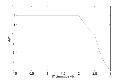
Figure 2: $d_{K}^{\ast}(0)$ as a function of the IC dimensions per channel use $K$, for $M=4$, $N=3$.

Figure 2 presents the maximal diversity order that can be attained for different average number of dimensions per channel use, for the case $M=4$ and $N=3$, i.e. the upper bound on the diversity order for $r=0$, $d^{\ast}_{K}(0)$, where $0\leq K\leq 3$. In the range $0\leq K\leq 2$ we get $d^{\ast}_{K}(0)=12$. It coincides with the result presented in Figure 1, where we showed that in this range the straight lines have the same value for $r=0$. Hence, for IC’s, one can use up to 2 average number of dimensions per channel use without compromising the diversity order. Starting from $K\geq 2$, the tradeoff starts to kick-in and the maximal diversity order starts to reduce as we increase the average number of dimensions per channel use. Also note that for $K=3$ the diversity order is $6$ when $r=0$.

IV Attaining the Best Diversity Order

In this section we show that the optimal DMT of finite constellations is achievable by a sequence of IC’s in general and lattices using regular lattice decoding in particular. In subsection IV-A we present a transmission scheme for any $M$ and $N$ that transmits an IC with $K_{l}=\frac{(M-l)(N-l)}{N+M-1-2\cdot l}+l$ and $T_{l}=N+M-1-2\cdot l$, $l=0,\dots,L-1$, where as previously defined $L=\min(M,N)$ and $K_{l}$ is chosen based on the results in section III. In subsection IV-B we present the effective channel induced by this transmission scheme. Following that we extend the methods presented in [13] and derive in Theorem 3 for each channel realization an upper bound on the average decoding error probability of ensemble of IC’s. By averaging the upper bound over the channel realizations, we show in Theorem 4 that the proposed transmission scheme attains the optimal DMT. In Theorem 5 we extend this result also to lattices when employing regular lattice decoder. Finally, we discuss power spreading technique over the transmit antennas for the transmission scheme in subsection IV-E, and give some averaging arguments on the existence of sequence of IC’s that attain the optimal DMT in subsection IV-F.

IV-A The Transmission Scheme

The transmission matrix $G_{l}$, $l=0,\dots,L-1$, has $M$ rows that represent the transmission antennas, and $T_{l}=N+M-1-2\cdot l$ columns that represent the number of channel uses.

We begin by describing the transmission matrix structure in general for any $M$ and $N$.

1. For $N\geq M$ and $K_{M-1}=\frac{M(N-M+1)}{N-M+1}=M$: the matrix $G_{M-1}$ has $N-M+1$ columns (channel uses). In the first column transmit symbols $x_{1},\dots,x_{M}$ on the $M$ antennas, and in the $N-M+1$ column transmit symbols $x_{M(N-M)+1},\dots,x_{M(N-M+1)}$ on the $M$ antennas.

2. For $M>N$ and $K_{N-1}=\frac{N(M-N+1)}{M-N+1}=N$: the matrix $G_{N-1}$ has $M-N+1$ columns. In the first column transmit symbols $x_{1},\dots,x_{N}$ on antennas $1,\dots,N$ and in the $M-N+1$ column transmit symbols $x_{N(M-N)+1},\dots,x_{N(M-N+1)}$ on antennas $M-N+1,\dots,M$.

3. For $K_{l}$, $l=0,\dots,L-2$: the matrix $G_{l}$ has $M+N-1-2\cdot l$ columns. We add to $G_{l+1}$, the transmission scheme of $K_{l+1}$, two columns in order to get $G_{l}$. In the first added column transmit $l+1$ symbols on antennas $1,\dots,l+1$. In the second added column transmit different $l+1$ symbols on antennas $M-l,\dots,M$.

Example: $M=4$, $N=3$. In this case the transmission scheme for $K=3$, $2.5$ and $2$ ($G_{2}$, $G_{1}$ and $G_{0}$ respectively) is as follows:

$$\underbrace{\underbrace{\underbrace{\left(\begin{array}[]{cc}x_{1}&0\\ x_{2}&x_{4}\\ x_{3}&x_{5}\\ 0&x_{6}\end{array}\right.}_{K_{2}=\frac{6}{2}}\left.\begin{array}[]{cc}x_{7}&0\\ x_{8}&0\\ 0&x_{9}\\ 0&x_{10}\end{array}\right.}_{K_{1}=\frac{10}{4}}\left.\begin{array}[]{cc}x_{11}&0\\ 0&0\\ 0&0\\ 0&x_{12}\end{array}\right)}_{K_{0}=\frac{12}{6}}.$$ (18)

IV-B The Effective Channel

Next we define the effective channel matrix induced by the transmission scheme. In accordance with the channel model from (4), the multiplication $H\cdot G_{l}$ yields a matrix with $N$ rows and $T_{l}$ columns, where each column equals to $H\cdot\underline{x}_{t}$, $t=1\dots T_{l}$, as in (4). We are interested in transmitting $K_{l}T_{l}$-complex dimensional IC with $K_{l}T_{l}$ complex symbols. Hence, in the proposed transmission scheme, $G_{l}$ has exactly $K_{l}T_{l}$ non-zero complex entries that represent the $K_{l}T_{l}$-complex dimensional IC within $\mathbb{C}^{MT_{l}}$. For each column of $G_{l}$, denoted by $\underline{g}_{i}$, $i=1\dots T_{l}$, we define the effective channel that $\underline{g}_{i}$ sees as $\widehat{H}_{i}$. It consists of the columns of $H$ that correspond to the non-zero entries of $\underline{g}_{i}$, i.e. $H\cdot\underline{g}_{i}=\widehat{H}_{i}\cdot\underline{\widehat{g}}_{i}$, where $\underline{\widehat{g}}_{i}$ equals the non-zero entries of $\underline{g}_{i}$. As an example assume without loss of generality that the first $l_{i}$ entries of $\underline{g}_{i}$ are not zero. In this case $\widehat{H}_{i}$ is an $N\times l_{i}$ matrix equals to the first $l_{i}$ columns of $H$. In accordance with (5), $H_{\mathrm{eff}}^{(l)}$ is an $NT_{l}\times K_{l}T_{l}$ block diagonal matrix consisting of $T_{l}$ blocks. Each block corresponds to the multiplication of $H$ with different column of $G_{l}$, i.e. $\widehat{H}_{i}$ is the $i^{\prime}th$ block of $H_{\mathrm{eff}}^{(l)}$. Note that in the effective matrix $NT_{l}\geq K_{l}T_{l}$.

We would like to elaborate on the structure of the blocks of $H_{\mathrm{eff}}^{(l)}$. For this reason we denote the columns of $H$ as $\underline{h}_{i}$, $i=1,\dots,M$.

1. The case where $N\geq M$. For this case the transmission scheme has $N+M-1-2\cdot l$ columns. The first $N-M+1$ columns of $G_{l}$, $\underline{g}_{1},\dots,\underline{g}_{N-M+1}$, contain $M\cdot(N-M+1)$ different complex symbols, i.e. there are no zero entries in these columns. Hence, in this case the first $N-M+1$ blocks of $H_{\mathrm{eff}}^{(l)}$ are

   $$\widehat{H}_{i}=H\qquad i=1,\cdots,N-M+1.$$ (19)

   After the first $N-M+1$ columns we have $M-1-l$ pairs of columns. For each pair we have

   $$\widehat{H}_{N-M+2k}=\{\underline{h}_{1},\dots,\underline{h}_{M-k}\}$$ (20)

   and

   $$\widehat{H}_{N-M+2k+1}=\{\underline{h}_{k+1},\dots,\underline{h}_{M}\}$$ (21)

   where $k=1,\dots,M-1-l$.

2. The case where $M>N$. Again the transmission scheme has $N+M-1-2\cdot l$ columns. By the definition of the first $M-N+1$ columns of $G_{l}$, we get that

   $$\widehat{H}_{i}=\{\underline{h}_{i},\dots,\underline{h}_{N+i-1}\}\qquad i=1,\cdots,M-N+1.$$ (22)

   We have additional $N-1-l$ pairs of columns in $G_{l}$. For each of these pairs we get

   $$\widehat{H}_{M-N+2k}=\{\underline{h}_{1},\dots,\underline{h}_{N-k}\}$$ (23)

   and

   $$\widehat{H}_{M-N+2k+1}=\{\underline{h}_{M-N+k+1},\dots,\underline{h}_{M}\}$$ (24)

   where $k=1,\dots,N-1-l$.

Example: consider $M=4$, $N=3$ as presented in (18). In this case $l=0,1,2$ and we have $K_{2}=3$, $K_{1}=2.5$ and $K_{0}=2$ respectively.

1. $K_{2}=3$: $H_{\mathrm{eff}}^{(2)}$ is generated from the multiplication of the $3\times 4$ matrix $H$ with the first two columns of the transmission matrix. In this case $H_{\mathrm{eff}}^{(2)}$ is a $6\times 6$ block diagonal matrix, consisting of two blocks. Each block is a $3\times 3$ matrix. We get that $\widehat{H}_{1}=\{\underline{h}_{1},\underline{h}_{2},\underline{h}_{3}\}$ and $\widehat{H}_{2}=\{\underline{h}_{2},\underline{h}_{3},\underline{h}_{4}\}$.

2. $K_{1}=\frac{10}{4}=2.5$: $H_{\mathrm{eff}}^{(1)}$ is a $12\times 10$ block diagonal matrix consisting of 4 blocks. The first two blocks are identical to the blocks of $H_{\mathrm{eff}}^{(2)}$. The additional two blocks (multiplication with columns 3-4) are $3\times 2$ matrices. We get that $\widehat{H}_{3}=\{\underline{h}_{1},\underline{h}_{2}\}$ and $\widehat{H}_{4}=\{\underline{h}_{3},\underline{h}_{4}\}$.

3. $K_{0}=2$: $H_{\mathrm{eff}}^{(0)}$ consists of six blocks. In this case the last two blocks are $3\times 1$ vectors. We get that $\widehat{H}_{5}=\underline{h}_{1}$ and $\widehat{H}_{6}=\underline{h}_{4}$.

We present $H_{\mathrm{eff}}^{(0)}$ of our example in equation (25). Note that $\underline{h}_{i}\in\mathbb{C}^{3}$ for $1\leq i\leq 4$, and $\underline{0}$ is a $3\times 1$ vector.

$$H_{\mathrm{eff}}^{(0)}=\left(\begin{array}[]{cccccc}\underline{h}_{1}&\underline{h}_{2}&\underline{h}_{3}&\underline{0}&\underline{0}&\underline{0}\\ \underline{0}&\underline{0}&\underline{0}&\underline{h}_{2}&\underline{h}_{3}&\underline{h}_{4}\\ \underline{0}&\underline{0}&\underline{0}&\underline{0}&\underline{0}&\underline{0}\\ \underline{0}&\underline{0}&\underline{0}&\underline{0}&\underline{0}&\underline{0}\\ \underline{0}&\underline{0}&\underline{0}&\underline{0}&\underline{0}&\underline{0}\\ \underline{0}&\underline{0}&\underline{0}&\underline{0}&\underline{0}&\underline{0}\end{array}\right.\left.\begin{array}[]{cccc}\underline{0}&\underline{0}&\underline{0}&\underline{0}\\ \underline{0}&\underline{0}&\underline{0}&\underline{0}\\ \underline{h}_{1}&\underline{h}_{2}&\underline{0}&\underline{0}\\ \underline{0}&\underline{0}&\underline{h}_{3}&\underline{h}_{4}\\ \underline{0}&\underline{0}&\underline{0}&\underline{0}\\ \underline{0}&\underline{0}&\underline{0}&\underline{0}\end{array}\right.\left.\begin{array}[]{cc}\underline{0}&\underline{0}\\ \underline{0}&\underline{0}\\ \underline{0}&\underline{0}\\ \underline{0}&\underline{0}\\ \underline{h}_{1}&\underline{0}\\ \underline{0}&\underline{h}_{4}\end{array}\right)$$ (25)

From the sequential construction of the blocks of $H_{\mathrm{eff}}^{(l)}$ (19)-(21), (22)-(24) it is easy to see that when two columns of $H$ occur in a certain block of $H_{\mathrm{eff}}^{(l)}$, the columns of $H$ between them must also occur in the same block, i.e. if $\underline{h}_{1}$, $\underline{h}_{5}$ occur in a certain block, then $\underline{h}_{2},\underline{h}_{3},\underline{h}_{4}$ also occur in the same block. Next we prove a property of the transmission scheme $G_{l}$, that relates to the number of occurrences of the columns of $H$ in the blocks of $H_{\mathrm{eff}}^{(l)}$. For each set of columns in $H$, we give an upper bound on the amount of its appearances in different blocks.

Lemma 1.

Consider the transmission scheme $G_{l}$, $l=0,\dots L-1$. In case $0\leq i-j<L$, the columns $\underline{h}_{j},\dots,\underline{h}_{i}$ may occur together in at most $N-i+j$ blocks of $H_{\mathrm{eff}}^{(l)}$. In case $i-j\geq L$ they can not occur together in any block of $H_{\mathrm{eff}}^{(l)}$.

Proof.

See appendix C. ∎

IV-C Upper Bound on The Error Probability

Next we would like to derive an upper bound on the average decoding error probability of ensemble of $K_{l}T_{l}$-complex dimensional IC, for each channel realization. We define $|H_{\mathrm{eff}}^{(l)\dagger}H_{\mathrm{eff}}^{(l)}|=\rho^{-\sum_{i=1}^{K_{l}T_{l}}\eta_{i}}$ , where $\rho^{-\frac{\eta_{i}}{2}}$ is the $i^{\prime}th$ singular value of $H_{\mathrm{eff}}^{(l)}$, $1\leq i\leq K_{l}T_{l}$. We also define $\underline{\eta}=(\eta_{1},\dots,\eta_{K_{l}T_{l}})^{T}$. Note that $NT_{l}\geq K_{l}T_{l}$.

Theorem 3.

There exists a sequence of $K_{l}T_{l}$-complex dimensional IC’s, with channel realization $H_{\mathrm{eff}}^{(l)}$ and a receiver VNR $\mu_{rc}=\rho^{1-\frac{r}{K_{l}}-\frac{\sum_{i=1}^{K_{l}T_{l}}{\eta_{i}}}{K_{l}T_{l}}}$, that has an average decoding error probability

$$\overline{P_{e}}(H_{\mathrm{eff}}^{(l)},\rho)=\overline{P_{e}}(\underline{\eta},\rho)\leq D(K_{l}T_{l})\rho^{-T_{l}(K_{l}-r)+\sum_{i=1}^{K_{l}T_{l}}\eta_{i}}=D(K_{l}T_{l})\rho^{-T_{l}(K_{l}-r)}\cdot|H_{\mathrm{eff}}^{(l)\dagger}H_{\mathrm{eff}}^{(l)}|^{-1}$$

where $D(K_{l}T_{l})$ is a constant independent of $\rho$, and $\eta_{i}\geq 0$ for every $1\leq i\leq K_{l}T_{l}$.

Proof.

We base our proof on the techniques developed by Poltyrev [13] for the AWGN channel. However, the channel considered here is colored. In spite of that, we show that what affects the average decoding error probability is the singular values product, which is encapsulated by the receiver VNR, $\mu_{rc}$. This observation enables us to facilitate this colored channel analysis. The full proof in appendix D. ∎

By averaging arguments we know that there exists a sequence of IC’s that satisfies these requirements.

IV-D Achieving the Optimal DMT

In this subsection we calculate the DMT of the proposed transmission scheme. We upper bound the determinant of the effective channel inverse, $|H_{\mathrm{eff}}^{(l)\dagger}H_{\mathrm{eff}}^{(l)}|^{-1}$, based on the effective channel properties presented in subsection IV-B. In Theorem 3 we showed that the upper bound on the error probability depends on this determinant. Hence, the upper bound on the determinant gives us a new upper bound on the average decoding error probability. We average the new upper bound over all channel realizations and get the DMT of the transmission scheme.

The channel matrix $H$ consists of $N\cdot M$ i.i.d entries, where each entry has distribution $h_{i,j}\sim CN(0,1)$. Without loss of generality we consider the case where the columns of $H$ are drawn sequentially from left to right, i.e. $\underline{h}_{1}$ is drawn first, then $\underline{h}_{2}$ is drawn et cetera. Column $\underline{h}_{j}$ is an $N$-dimensional vector. Given $\underline{h}_{\max(1,j-N+1)},\dots,\underline{h}_{j-1}$, we can write

$$\underline{h}_{j}=\Theta(\underline{h}_{\max(1,j-N+1)},\dots,\underline{h}_{j-1})\cdot\underline{\widetilde{h}}_{j}$$

where $\Theta(\cdot)$ is an $N\times N$ unitary matrix. $\Theta(\cdot)$ is chosen such that:

1. The first element of $\underline{\widetilde{h}}_{j}$, $\widetilde{h}_{1,j}$, is in the direction of $\underline{h}_{j-1}$.

2. The second element, $\widetilde{h}_{2,j}$, is in the direction orthogonal to $\underline{h}_{j-1}$, in the hyperplane spanned by $\{\underline{h}_{j-1},\underline{h}_{j-2}\}$.

3. Element $\widetilde{h}_{\min(j,N)-1,j}$ is in the direction orthogonal to the hyperplane spanned by $\{\underline{h}_{\max(2,j-N+2)},\dots,\underline{h}_{j-1}\}$ inside the hyperplane spanned by $\{\underline{h}_{\max(1,j-N+1)},\dots,\underline{h}_{j-1}\}$.

4. The rest of the $N-\min(j,N)+1$ elements are in directions orthogonal to the hyperplane $\{\underline{h}_{\max(1,j-N+1)},\dots,\underline{h}_{j-1}\}$.

Note that $\widetilde{h}_{i,j}$, $1\leq i\leq N$, $1\leq j\leq M$ are i.i.d random variables with distribution $CN(0,1)$. Let us denote by $\underline{h}_{j\perp j-1,\dots,j-k}$ the component of $\underline{h}_{j}$ which resides in the $N-k$ subspace which is perpendicular to the space spanned by $\{\underline{h}_{j-1},\dots,\underline{h}_{j-k}\}$. In this case we get

$$\lVert\underline{h}_{j\perp j-1,\dots,j-k}\rVert^{2}=\sum_{i=k+1}^{N}|\widetilde{h}_{i,j}|^{2}\quad 1\leq k\leq\min(j,N)-1.$$ (26)

If we assign $|\widetilde{h}_{i,j}|^{2}=\rho^{-\xi_{i,j}}$, we get that the probability density function (PDF) of $\xi_{i,f}$ is

$$f(\xi_{i,j})=C\cdot\log{\rho}\cdot\rho^{-\xi_{i,j}}\cdot e^{-\rho^{-\xi_{i,j}}}$$ (27)

where $C$ is a normalization factor. In our analysis we assume a very large value for $\rho$. Hence we can neglect events where $\xi_{i,j}<0$ since in this case the PDF (27) decreases exponentially as a function of $\rho$. For a very large $\rho$, $\xi_{i,j}\geq 0$, $1\leq i\leq N$ and $1\leq j\leq M$, the PDF takes the following form

$$f(\xi_{i,j})\propto\rho^{-\xi_{i,j}}\qquad\xi_{i,j}\geq 0.$$ (28)

In this case by assigning in (26) the vector $\underline{\xi}_{j}=(\xi_{1,j},\dots,\xi_{N,j})^{T}$, whose PDF is proportional to $\rho^{-\sum_{i=1}^{N}\xi_{i,j}}$, we get

$$\lVert\underline{h}_{j\perp j-1,\dots,j-k}\rVert^{2}\dot{=}\rho^{-\min_{s\in\{k+1,\dots,N\}}\xi_{s,j}}=\rho^{-a(k,\underline{\xi}_{j})}$$ (29)

where $1\leq k\leq\min(j,L)-1$ and $a(k,\underline{\xi}_{j})=\min_{s\in\{k+1,\dots,N\}}\xi_{s,j}$. In addition

$$\lVert\underline{h}_{j}\rVert^{2}\dot{=}\rho^{-\min_{s\in\{1,\dots,N\}}\xi_{s,j}}=\rho^{-a(0,\underline{\xi}_{j})}.$$ (30)

Note that

$$a(\min(j,L)-1,\underline{\xi}_{j})\geq\dots\geq a(0,\underline{\xi}_{j})\geq 0.$$ (31)

Next we wish to quantify the contribution of a certain column in the channel matrix, $\underline{h}_{j}$, to the determinant $|H_{\mathrm{eff}}^{(l)\dagger}H_{\mathrm{eff}}^{(l)}|$. $H_{\mathrm{eff}}^{(l)}$ is a block diagonal matrix. Hence the determinant of $|H_{\mathrm{eff}}^{(l)\dagger}H_{\mathrm{eff}}^{(l)}|$ can be expressed as

$$|H_{\mathrm{eff}}^{(l)\dagger}H_{\mathrm{eff}}^{(l)}|=\prod_{i=1}^{T_{l}}|\widehat{H}_{i}^{\dagger}\widehat{H}_{i}|.$$ (32)

Assume $\widehat{H}_{i}=(\underline{\widehat{h}}_{1},\dots,\underline{\widehat{h}}_{m})$, i.e. $\widehat{H}_{i}$ has $m$ columns. In this case we can state that the determinant

$$|\widehat{H}_{i}^{\dagger}\widehat{H}_{i}|=\lVert\underline{\widehat{h}}_{1}\rVert^{2}\lVert\underline{\widehat{h}}_{2\perp 1}\rVert^{2}\dots\lVert\underline{\widehat{h}}_{m\perp m-1,\dots,1}\rVert^{2}.$$

Note that $\widehat{H}_{i}$ also has more rows than columns. The columns of $\widehat{H}_{i}$ are subset of the columns of the channel matrix $H$. Hence we are interested in the blocks where $\underline{h}_{j}$ occurs. We know that the contribution of $\underline{h}_{j}$ to those determinants can be quantified by taking into account the columns to its left in each block. We consider two cases:

• The case $N\geq M$. In this case we can see from (19)-(21) that $\underline{h}_{j}$ may occur with $\{\underline{h}_{1},\dots,\underline{h}_{j-1}\}$ to its left in different blocks.

• The case $M>N$. In this case we can see from (22)-(24) that $\underline{h}_{j}$ may occur only with $\{\underline{h}_{\max(1,j-N+1)},\dots,\underline{h}_{j-1}\}$ to its left in different blocks.

Based on (29) and (30) we can quantify the contribution of $\underline{h}_{j}$ to $|H_{\mathrm{eff}}^{(l)\dagger}H_{\mathrm{eff}}^{(l)}|$ by

$$\lVert\underline{h}_{j}\rVert^{2b_{j}(0)}\prod_{k=1}^{\min(j,L)-1}\lVert\underline{h}_{j\perp j-1,\dots,j-k}\rVert^{2b_{j}(k)}\dot{=}\rho^{-\sum_{k=0}^{\min(j,L)-1}b_{j}(k)a(k,\underline{\xi}_{j})}$$ (33)

where $b_{j}(k)$ is the number of occurrences of $\underline{h}_{j}$ in the blocks of $H_{\mathrm{eff}}^{(l)}$, with only $\{\underline{h}_{j-1},\dots,\underline{h}_{j-k}\}$ to its left. $b_{j}(0)$ is the number of occurrences of $\underline{h}_{j}$ with no columns to its left. Note that from the definition of the transmission scheme we get that for $l=0$, $b_{j}(k)>0$ for $1\leq k\leq\min(j,L)-1$.

In the following theorem we calculate the DMT of the proposed transmission scheme.

Theorem 4.

There exists a sequence of $K_{l}T_{l}$-complex dimensional IC’s with transmitter density $\gamma_{tr}=\rho^{rT_{l}}$ and $T_{l}$ channel uses that has diversity order

$$d_{K_{l}T_{l}}(r)\geq(M-l)(N-l)-(r-l)(N+M-2\cdot l-1)$$

where $0\leq r\leq K_{l}$ and $l=0,\dots,L-1$. In the range $l\leq r\leq l+1$ this lower bound coincides with the optimal DMT of finite constellations.

Proof.

The proof outline is as follows. The upper bound on the error probability from Theorem 3 depends on $|H_{\mathrm{eff}}^{(l)\dagger}H_{\mathrm{eff}}^{(l)}|^{-1}$. We upper bound this determinant value and average over different realizations of $H_{\mathrm{eff}}^{(l)}$ in order to find the diversity order of the transmission matrix $G_{l}$. We begin by lower bounding $|H_{\mathrm{eff}}^{(l)\dagger}H_{\mathrm{eff}}^{(l)}|$. Based on the sequential structure of $G_{l}$, we lower bound the contribution of a certain column of $H$, $\underline{h}_{j}$, $1\leq j\leq M$ to the determinant. This gives us a new upper bound on the error probability for each channel realization. We average the new upper bound on the error probability, by averaging over $\underline{\widetilde{h}}_{1},\dots,\underline{\widetilde{h}}_{M}$. From this averaging we get the required DMT. The full proof is in appendix E ∎

The diversity order attained in Theorem 4 for $K_{l}$, $T_{l}$ coincides with the optimal DMT of finite constellations in the range $l\leq r\leq l+1$. Hence, by considering $0\leq l\leq L-1$, we can attain the optimal DMT with $L$ sequences of IC’s.

We present as an illustrative example the case of $M=N=2$. Let us consider the case where $l=0$. In this case $K_{0}=\frac{4}{3}$, and $T_{0}=3$, i.e. we transmit $4$-complex dimensional IC. The transmission scheme diversity order in this case is $4-3r$, $0\leq r\leq\frac{4}{3}$. In this case the effective channel matrix, $H_{\mathrm{eff}}^{(0)}$, consists of three blocks: $\widehat{H}_{1}=(\underline{h}_{1},\underline{h}_{2})$, $\widehat{H}_{2}=\underline{h}_{1}$ and $\widehat{H}_{3}=\underline{h}_{2}$. According to our definitions

$$|\widehat{H}_{1}^{\dagger}\widehat{H}_{1}|=\lVert\underline{h}_{1}\rVert^{2}\cdot\lVert\underline{h}_{2\perp 1}\rVert^{2}=\rho^{-\min(\xi_{1,1},\xi_{2,1})}\cdot\rho^{-\xi_{2,2}}$$

and also $\lVert\underline{h}_{1}\rVert^{2}=\rho^{-\min(\xi_{1,1},\xi_{2,1})}$, $\lVert\underline{h}_{2}\rVert^{2}=\rho^{-\min(\xi_{1,2},\xi_{2,2})}$. In accordance with (83) we divide the integral into two terms. In the first term we solve the optimization problem

$$\min_{\xi_{\underline{i},\underline{j}}\in\mathcal{A}}(4-3r)-(\xi_{2,2}+2\cdot\min{\big{(}\xi_{1,1},\xi_{2,1})}+\min{(\xi_{1,2},\xi_{2,2}})\big{)}+\sum_{i=1}^{2}\sum_{j=1}^{2}\xi_{i,j}.$$ (34)

One solution to this problem is $\xi_{i,j}=0$ for $1\leq i\leq 2$, $1\leq j\leq 2$. In this case we get an exponential term that equals $4-3r$. For the second integral we solve the optimization problem

$$\min_{\xi_{\underline{i},\underline{j}}\in\overline{\mathcal{A}}}\sum_{i=1}^{2}\sum_{j=1}^{2}\xi_{i,j}.$$

In this case the optimization problem solution is $\sum_{i=1}^{2}\sum_{j=1}^{2}\xi_{i,j}=4-3r$. Hence, all together, we get a diversity order that equals $4-3r$, that coincides with the optimal DMT of finite constellations in the range $0\leq r\leq 1$.

In the next theorem we prove the existence of a sequence of lattices that has the same lower bound as in Theorem 4.

Theorem 5.

There exists a sequence of $2K_{l}T_{l}$-real dimensional lattices with transmitter density $\gamma_{tr}=\rho^{rT_{l}}$ and $T_{l}$ channel uses, that attains a diversity order

$$d_{K_{l}T_{l}}(r)\geq(M-l)(N-l)-(r-l)(N+M-2\cdot l-1)$$

where $0\leq r\leq K_{l}$ and $l=0,\dots,L-1$.

Proof.

See appendix G ∎

Note that we considered a $2K_{l}T_{l}$-real dimensional lattice, where the lattice first $K_{l}T_{l}$ dimensions are spread over the real part of the non-zero entries of $G_{l}$, and the other $K_{l}T_{l}$ dimensions of the lattice are spread on the imaginary part of the non-zero entries of $G_{l}$. This does not necessarily yields a $K_{l}T_{l}$-complex dimensional lattice in the transission scheme. Considering the $2K_{l}T_{l}$-real dimensional lattice enables us to use the Minkowski-Hlawaka-Siegel Theorem [13],[19], and prove Theorem 5.

IV-E Power Spreading

For practical reasons, such as power peak to average ratio, one may prefer to have a transmission scheme that spreads the transmitted power equally over time and space. The transmitting matrix $G_{l}$ contains exactly $K_{l}T_{l}$ non-zero entries, where the rest of the entries are zero. In order to spread the power more equally over time and space we use the following unitary operations

$$U_{L}G_{l}U_{R}.$$

$U_{L}$ is an $M\times M$ unitary matrix that spreads each column of $G_{l}$, i.e. spreads over space. $U_{R}$ is a $T_{l}\times T_{l}$ unitary matrix that spreads each raw of $G_{l}$, i.e. spreads over time. As the distribution of $H$ and $H\cdot U_{L}$ are identical, multiplying $U_{L}$ with $G_{l}$ gives exactly the same performance. Based on the notations from $\eqref{eq:Channel Fading}$ we can state that

$$G_{l}\cdot U_{R}=\big{(}\underline{x}_{1},\dots,\underline{x}_{T_{l}}\big{)}$$

where $\big{(}\underline{x}_{1},\dots,\underline{x}_{T_{l}}\big{)}$ are the channel inputs. In the receiver we can state that the received signals are $\big{(}\underline{y}_{1},\dots,\underline{y}_{T_{l}}\big{)}$. By multiplying with $U_{R}^{\dagger}$ we get

$$\big{(}\underline{y}_{1},\dots,\underline{y}_{T_{l}}\big{)}\cdot U_{R}^{\dagger}=G_{l}+\big{(}\underline{n}_{1},\dots,\underline{n}_{T_{l}}\big{)}U_{R}^{\dagger}.$$

The distribution of $\big{(}\underline{n}_{1},\dots,\underline{n}_{T_{l}}\big{)}$ is identical to the distribution of $\big{(}\underline{n}_{1},\dots,\underline{n}_{T_{l}}\big{)}U_{R}^{\dagger}$. Hence, multiplying $G_{l}$ with $U_{R}$ gives also exactly the same performance. For instance, in order to achieve full diversity and spread the power more uniformly, we take $G_{0}$ and duplicate its structure $s$ times to create the transmission scheme $G_{0}^{(s)}$. In this case the transmission matrix $G_{0}^{(s)}$ consists of $sK_{0}T_{0}$ complex non-zero entries, i.e we transmit an $sK_{0}T_{0}$ complex dimensional IC within the $sMT_{0}$ complex space. $G_{0}^{(s)}$ is an $M\times sT_{0}$ dimensional matrix, that has exactly the same diversity order as $G_{0}$ (it duplicates the structure of $G_{0}$ $s$ times). Each row of $G_{0}^{(s)}$ has exactly $sN$ non-zero entries. We define $U_{R}^{(s)}$ as $sT_{0}\times sT_{0}$ unitary matrix. For large enough $s$, the multiplication $G_{0}^{(s)}\cdot U_{R}^{(s)}$ spreads the power more uniformly over space and time, and still achieves full diversity.

IV-F Averaging Arguments

In this subsection we show that there exist $L$ sequences of lattices that attain the optimal DMT, where each sequence of the $L$ sequences attains a different segment on the optimal DMT curve. In addition we show that there exists a single IC that attains the optimal DMT by diluting its points and adapting its dimensionality.

As a consequence of Theorem 3 and Theorem 4 we can state the following

Corollary 3.

Consider a sequence of $KT$-complex dimensional IC’s $S_{KT}(\rho)$ with density $\gamma_{tr}=1$, that attains diversity order $d$. This sequence of IC’s also attains diversity order $d(1-\frac{r}{K})$ when the sequence density is scaled to $\gamma_{tr}=\rho^{rT}$.

Proof.

The proof is in appendix H. ∎

Corollary 4.

The optimal DMT is attained by exactly $L$ sequences of $2K_{l}T_{l}$-real dimensional lattices, $l=0,\dots,L-1$, where each sequence attains different segment of the optimal DMT.

Proof.

From Theorem 5 we know that there exists a $2K_{l}T_{l}$-real dimensional sequence of lattices with density $\gamma_{tr}=1$ that attains diversity $(M-l)(N-l)+l(N+M-2\cdot l-1)$. Hence, based on Corollary 3 we can scale this $2K_{l}T_{l}$-real dimensional sequence of lattices into a sequence of lattices with density $\gamma_{tr}=\rho^{rT_{l}}$, and a diversity order $(M-l)(N-l)-(r-l)(N+M-2\cdot l-1)$, i.e. the sequence of lattices attains the optimal DMT line in the range $l\leq r\leq l+1$. The optimal DMT is the maximal value of the $L$ lines, for each $0\leq r\leq L$. Hence, there exist $L$ sequences of lattices that attain the optimal DMT. ∎

Next, we show that there exists a single sequence of IC’s that attains the optimal DMT. The optimal DMT consists of $L$ segments of straight lines. Each segment is attained by reducing the IC’s dimensionality to the correct dimension, and diluting their points to get the desired density. Note that in Theorem 4 we showed that for each multiplexing gain, $r$, there exists a sequence of IC’s that attains the optimal DMT. On the other hand, in Corollary 5 we show that a single sequence of IC’s attains the optimal DMT for any $r$, by adapting its dimensionality and diluting its points. Also note that $K_{0}T_{0}>K_{1}T_{1}>\cdots>K_{L-1}T_{L-1}$.

Corollary 5.

There exists a single sequence of $K_{0}T_{0}$-complex dimensional IC’s, that attains the $L$ segments of the optimal DMT:

$$(M-l)(N-l)-(r-l)(N+M-2\cdot l-1)\quad 0\leq r\leq K_{l}$$

where $l=0,\cdots,L-1$. The $l^{\prime}th$ segment is attained by reducing the IC’s complex dimensionality to $K_{l}T_{l}$, and by diluting their points to get density $\gamma_{tr}=\rho^{T_{l}r}$.

Proof.

See Appendix I. ∎

V Discussion

In this section we discuss the results presented in the paper. We begin by explaining why full dimension lattice based coding schemes such as Golden-codes [9], perfect codes [10] and other cyclic-division algebra based space-time codes [6] which were shown to attain the optimal DMT, are sub-optimal when regular lattice decoder (3) is employed in the receiver. In addition, we explain why using the MMSE estimation in the receiver enables these schemes to attain the optimal DMT. Afterwards, based on our results, we give another geometrical interpretation to the optimal DMT. Finally, since in practice a finite codebook is transmitted, we show that given a lattice with multiplexing gain $r$ as defined for IC’s in (6), a finite constellation with multiplexing gain $r$ as defined in [3] can also be carved from it.

V-A Lattice Constellations Vs. Full Dimension Lattice Based Finite Constellations

In order to demonstrate that full dimension lattice based coding schemes with regular lattice decoding are sub-optimal let us consider Golden-codes transmitted over a channel with $M=N=2$ where $T=2$. For large $\rho$ the channel singular values PDF is proportional to $\rho^{-\alpha_{1}-3\alpha_{2}}$, where $\alpha_{1}\geq\alpha_{2}\geq 0$. A Golden-code of a certain rate is carved from a $4$-complex dimensional lattice. We show that when performing regular lattice decoding in the receiver the maximal diversity order that can be attained for $r=0$ is $2$. This is in contrast to ML decoding or alternatively MMSE estimation followed by lattice decoding [7], [8] for which the maximal diversity order equals 4.

We begin by showing why the maximal diversity order of a Golden-code is 2 when performing regular lattice decoding. In the receiver, the squared effective radius of the effective lattice induced by the channel realization equals (1)

$$r_{\mathrm{eff}}^{2}\dot{=}\rho^{-\frac{\alpha_{1}+\alpha_{2}}{2}}\dot{=}\gamma_{\mathrm{rc}}^{-\frac{1}{4}}.$$ (35)

For lattices $r_{\mathrm{eff}}\geq r_{\mathrm{packing}}=\frac{d_{\min}^{\left(\mathrm{lattice}\right)}}{2}$, where $r_{\mathrm{packing}}$, $d_{\min}^{\left(\mathrm{lattice}\right)}$ are the packing radius and the minimal distance of the lattice respectively. Hence, we get

$$\left(\frac{d_{\min}^{\left(\mathrm{lattice}\right)}}{2}\right)^{2}\dot{\leq}\rho^{-\frac{\alpha_{1}+\alpha_{2}}{2}}.$$ (36)

When the squared minimal distance is in the order of the additive noise variance, $\rho^{-1}$, the error probability will not decrease with $\rho$. This will happen for instance when $\alpha_{2}=0$ and $\alpha_{1}=2$. This event occurs for large $\rho$ with probability proportional to $\rho^{-2}$. Hence, in this case the diversity order is 2. Note that for the 4-complex dimensional lattice we get (9)

$$\mu_{\mathrm{rc}}\dot{=}\frac{r_{\mathrm{eff}}^{2}}{\rho^{-1}}\dot{=}\rho^{1-\frac{\alpha_{1}+\alpha_{2}}{2}}.$$ (37)

Therefore, the event where the squared effective radius is in the order of the noise variance is equivalent to $\mu_{\mathrm{rc}}\dot{=}1$ which is the outage event for lattices, presented in Theorem 2.

From equation (36) we get that the minimal distance for each channel realization of the entire lattice, induces diversity order 2. On the other hand, when the decoder only considers the words within the finite codebook, the non-vanishing determinant (NVD) property combined with the boundaries of the codebook leads to a lower bound on the minimal distance of the Golden-code for each channel realization, that is larger than the expression in (36), and enables to attain diversity order 4 [6].

The fact that considering the entire lattice leads to smaller minimal distance is not surprising since the multiplication of the transmitted lattice with the channel realization leads to scaling of this lattice in the direction of the channel singular values. When considering the infinite lattice, the scaling may reduce the distance between points that were very far in the transmitted lattice. These points are not necessarily part of the finite codebook and therefore does not effect the minimal distance of the finite Golden-code but do effect the minimal distance of the lattice.

MMSE estimation followed by lattice decoding will also lead to diversity order 4. Translating the arguments presented in [7], [8] to our setting leads to VNR

$$\tilde{\mu}_{\mathrm{rc}}\dot{=}\rho^{\frac{\left(1-\alpha_{1}\right)^{+}+\left(1-\alpha_{2}\right)^{+}}{2}}$$ (38)

where $\left(x\right)^{+}=x$ for $x\geq 0$ and zero else. This expression is larger than the expression in (37) and implies that the MMSE estimation, that takes into account the transmitted power, also improves the minimal distance for each channel realization. However, the improvement in VNR (and minimal distance) comes at the expense of a self additive noise that depends on the transmitted codeword. Under the assumption that the transmitted codewords are not too far from the origin the variance of the effective noise is small enough to allow attaining the optimal DMT. For instance Golden-code codewords are from a bounded shaping region, which enables to attain diversity order 4. Note that for the entire lattice, the farther the lattice point is from the origin, the larger the effective noise variance is. This eventually leads to poor error performance for lattice points far enough from the origin.

Our work shows that transmitting a lattice with average number of dimensions per channel use $K=\frac{4}{3}$ and performing regular lattice decoding in the receiver leads to VNR

$$\mu_{\mathrm{rc}}\dot{=}\rho^{1-\frac{\alpha_{1}}{4}-\frac{3\alpha_{2}}{4}}$$ (39)

which is also larger than (37) and enables to attain diversity order 4 (in fact it attains the optimal DMT in the range $0\leq r\leq 1$). Hence, from our work we can see that reducing the lattice dimensionality increases the lattice minimal distance to such an extent that enables to attain the optimal DMT when performing regular lattice decoding. In this sense reducing the lattice dimensionality takes the role of MMSE estimation. It is also interesting to note that MMSE estimation followed by lattice decoding yields good error performance for lattice points close enough to the origin (for instance lattice points within the shaping region), and bad performance for lattice points very far from the origin. On the other hand, regular lattice decoding yields the same performance for all lattice points inside or outside the shaping region. An illustrative example that shows how reduced dimension assists in increasing the minimal distance compared to full dimension lattice is presented in Figure 3.

(a) Finite constellation: In this case even when $h_{2}$ is small it is possible to decode.

(b) Full dimensional infinite constellaion: In this case due to the infiniteness of the constellation when $h_{2}$ is very small it is impossible to decode.

(c) Infinite constellaion with reduced dimension: In this case even when $h_{2}$ is very small it is possible to decode.

Figure 3: Illustrative example for the case $M=2$, $N=2$ of the significance of reducing dimensions when considering regular lattice decoding. For this example we assume that the realization of $H$ is diagonal, where the diagonal elements are $h_{1}$ and $h_{2}$.

V-B Geometrical Interpretation of the Optimal DMT, for IC’s

In this subsection we give a geometrical interpretation of the optimal DMT, based on allocation of lattice dimensions. This is a qualitative discussion and the exact results appear in sections III, IV.

First from our results we can see that for a sequence of lattices with certain number of dimensions per channel use the DMT is a straight line as a function of the multiplexing gain (see Corollary 3). It results from the fact that for lattices changing the multiplexing gain is equivalent to scaling each dimension by $\rho^{-\frac{r}{2K}}$. Assume that the sequence of lattices attains for multiplexing gain $r=0$ diversity order $d$, i.e. the error probability decays as $\rho^{-d}$. In this case scaling each dimension by $\rho^{-\frac{r}{2K}}$ leads to error probability that decays as $\rho^{-d\left(1-\frac{r}{K}\right)}$. This behavior results from the fact that the lattice decoder takes into consideration all the lattice points. Hence, the scaling merely replaces $\rho$ with $\rho^{1-\frac{r}{K}}$ in the error probability expression. The optimal DMT is a piecewise linear function. We get that each line corresponds to a sequence of lattices with certain number of dimensions per channel use.

Next we wish to give the reasoning for the average number of dimensions per channel use required to achieve each line in the optimal DMT. For simplicity let us consider the case $M=N=3$. We begin by considering the straight line in the range $0\leq r\leq 1$. In this range the optimal DMT equals $9-5\cdot r$. We wish to show why the average number of dimensions per channel use that enables to attain this straight line equals $\frac{9}{5}$. For large $\rho$ the channel singular values PDF is of the form of $\rho^{-\alpha_{1}-3\alpha_{2}-5\alpha_{3}}$, where $\alpha_{1}\geq\alpha_{2}\geq\alpha_{3}\geq 0$. When the transmission scheme spreads over $T$ channel uses, the equivalent channel matrix, $H_{\mathrm{ex}}$, presented in (5) has $3T$ singular values. Each singular value of $H$ occurs $T$ times in the singular values of $H_{\mathrm{ex}}$. Assume each complex dimension of the lattice is transmitted on a certain singular value of $H_{\mathrm{ex}}$. Let us denote by $T_{i}$ the number of dimensions transmitted on the singular values that equal $\rho^{-\frac{\alpha_{i}}{2}}$, $1\leq i\leq 3$. Note that $\sum_{i=1}^{3}T_{i}$ may be smaller than $3T$. According to this assumption a $\left(\sum_{i=1}^{3}T_{i}\right)$-complex dimensional lattice is transmitted over $T$ channel uses, and the average number of dimensions per channel use is $K=\frac{\sum_{i=1}^{3}T_{i}}{T}$. The effective radius in the receiver equals

$$r_{\mathrm{eff}}\dot{=}\rho^{-\frac{r\cdot T}{\sum_{i=1}^{3}T_{i}}-\frac{T_{1}\alpha_{1}+T_{2}\alpha_{2}+T_{3}\alpha_{3}}{\sum_{i=1}^{3}T_{i}}}.$$ (40)

and the VNR equals

$$\mu_{\mathrm{rc}}\dot{=}\rho^{1-\frac{r\cdot T}{\sum_{i=1}^{3}T_{i}}-\frac{T_{1}\alpha_{1}+T_{2}\alpha_{2}+T_{3}\alpha_{3}}{\sum_{i=1}^{3}T_{i}}}.$$ (41)

We are interested in the probability of the outage event, i.e. the probability that $\mu_{\mathrm{rc}}\dot{=}1$. Essentially, we show that when $K<\frac{9}{5}$ it is possible to attain maximal diversity order of $9$ for $r=0$, but it is impossible to attain the line $9-5\cdot r$ for any $0<r\leq\frac{9}{5}$. It results from the fact that multiplexing gain $r>0$ requires scaling each dimension by $\rho^{-\frac{r}{2K}}=\rho^{-\frac{r\cdot T}{2\sum_{i=1}^{3}T_{i}}}$, which decreases $r_{\mathrm{eff}}$ (and as a consequence also decreases the lattice minimal distance) to such an extent that it does not enable to attain the optimal DMT. On the other hand when $K>\frac{9}{5}$ the channel decreases $r_{\mathrm{eff}}$ to such an extent that it does not enable to attain the optimal DMT for $0\leq r<1$. Hence, $K=\frac{9}{5}$ balances the effect of the scaling and the channel and allows to attain the optimal DMT in the range $0\leq r\leq 1$.

In order to attain the maximal diversity order $9$ when $r=0$, the outage event $\mu_{\mathrm{rc}}\dot{=}1$ implies that the following conditions need to be fulfilled

$$\frac{T_{1}}{\sum_{i=1}^{3}T_{i}}\leq\frac{1}{9},\qquad\frac{T_{1}+T_{2}}{\sum_{i=1}^{3}T_{i}}\leq\frac{4}{9}$$ (42)

i.e. each singular value can not occur in more dimensions than the relative effect it has on the PDF of the singular values. The largest average number of dimensions per channel use that fulfils (42) is $\frac{9}{5}$. In this case for $T=5$ a 9-complex dimensional lattice is transmitted, and the conditions are fulfilled with equality when $T_{1}=1$, $T_{2}=3$ and $T_{3}=5$. When $K<\frac{9}{5}$ the conditions in (42) are still fulfilled and therefore diversity order $9$ is still attained for $r=0$. However, based on (40) we get for $r>0$ that $r_{\mathrm{eff}}$ decreases faster than the case of $K=\frac{9}{5}$. Hence, for $K<\frac{9}{5}$ the diversity order is smaller than $9-5\cdot r$ when $0<r\leq\frac{9}{5}$.

So far we have shown that choosing $K<\frac{9}{5}$ leads to sub-optimal DMT. Now, we wish to show that in the range $0\leq r\leq 1$ the DMT is smaller than $9-5\cdot r$ also when $K>\frac{9}{5}$. First, for $K>\frac{9}{5}$ the conditions in (42) are not met. Hence, in this case the diversity order is smaller than $9$ when $r=0$. For $r=1$ and $K=\frac{9}{5}$ the diversity order equals $4$. Assume the best assignment of lattice dimensions would enable to choose $T_{3}=T$. In this case $\mu_{\mathrm{rc}}$ in (41) is effected equally if $r=1$, $\alpha_{3}=0$ or $r=0$, $\alpha_{3}=1$, i.e. the scaling inflicted by $r=1$ decreases $r_{\mathrm{eff}}$ in (40) as if the singular value $\rho^{-\frac{\alpha_{3}}{2}}=\rho^{-\frac{1}{2}}$. In both cases we get

$$\mu_{\mathrm{rc}}=\rho^{\frac{T_{1}+T_{2}-T_{1}\alpha_{1}-T_{2}\alpha_{2}}{T_{1}+T_{2}+T}}.$$ (43)

The difference is that when $r=1$, $\alpha_{3}=0$ the PDF of the singular values equals $\rho^{-\alpha_{1}-3\alpha_{2}}$ which leads to smaller diversity order than the case $r=0$, $\alpha_{3}=1$. For large $\rho$ and $r=1$, $\alpha_{3}=0$ is included in the most dominant error event when $K\geq\frac{9}{5}$. Hence, diversity order of $4$ is attained for $r=1$ and $K>\frac{9}{5}$ when the following condition is met

$$\frac{T_{1}}{T_{1}+T_{2}}\leq\frac{1}{4}$$ (44)

which is exactly the condition for attaining maximal diversity order of $4$ when $r=0$ in a channel with $2$ transmit and $2$ receive antennas. This condition is met as long as $K\leq\frac{7}{3}$. Hence, for $\frac{9}{5}<K\leq\frac{7}{3}$ the best diversity order is smaller than $9$ when $r=0$, and equals $4$ when $r=1$. Since for each $K$ the largest DMT is a straight line, the DMT for each $0<K\leq\frac{7}{3}$ in the range $0\leq r\leq 1$ is smaller than $9-5\cdot r$. We are left with the case $\frac{7}{3}<K\leq 2$. By applying similar arguments, only this time considering $r=2$, it can be shown that in the range $0\leq r<2$ the largest DMT for any $\frac{7}{3}<K\leq 2$ is smaller than $7-3\cdot r$. These arguments also show that in the range $2\leq r\leq 3$ the optimal DMT equals $2-r$. Hence, we get for $0\leq r<1$ that the optimal DMT equals $9-5\cdot r$, where for $1\leq r<2$, $2\leq r\leq 3$ the optimal DMT equals $7-3\cdot r$ and $2-r$ respectively.

V-C The Relation Between the Multiplexing Gains of an IC and a Finite Constellation

In this paper we defined the multiplexing gain of IC’s sequence as the rate the IC’s density increases (6), i.e. when $\gamma_{\mathrm{tr}}=\rho^{rT}$ the multiplexing gain is $r$. We characterized the optimal DMT of IC’s based on this definition of the multiplexing gain. In practice a finite constellation is transmitted, even when performing regular lattice decoding in the receiver. Hence, in this subsection we show that finite constellation with multiplexing gain $r$ can be carved from a lattice with multiplexing gain $r$ (according to the definition given in (6)), while maintaining the same performance when performing regular lattice decoding in the receiver.

Consider a lattice $\Lambda$ with density $\gamma_{\mathrm{tr}}=\rho^{rT}$. In this case for each lattice point the Voronoi region volume equals

$$|V\left(x\right)|=|V|=\gamma_{\mathrm{tr}}^{-1}=\rho^{-rT}\quad\forall x\in\Lambda.$$

In [20] it has been shown that for any Jordan measurable bounded set $S$ with volume $|V\left(S\right)|$ there exists a translate $u$ such that

$$|\left(\Lambda+u\right)\cap S|\geq\frac{|V\left(S\right)|}{|V|}$$ (45)

where $\Lambda+u$ is the translate of each lattice point by the constant $u$, and $|\left(\Lambda+u\right)\cap S|$ is the number of words of the translated lattice within the region $S$. Hence, for each lattice in a sequence with multiplexing gain $r$, there exists a translate such that the number of codewords within a sphere with volume 1 is larger or equal to $\rho^{rT}$, i.e. the rate is $r\log\left(\rho\right)$ where in this setting $\rho$ takes the role of $\mathsf{SNR}$. Hence, it is possible to carve from the translated lattices sequence a finite constellations sequence with multiplexing gain $r$ according to the definitions of finite constellations. When performing regular lattice decoding the translate does not effect the performance. Hence, the results we presented in this work also apply when carving finite constellations with the corresponding multiplexing gain from the lattices sequence, and performing regular lattice decoding in the receiver.

VI Summary

This work investigates the DMT of IC’s. A new tradeoff between the IC average number of dimensions per channel use and the best DMT it may attain is presented. Based on this tradeoff a transmission scheme that enables to attain the optimal DMT of finite constellations, by lattices with regular lattice decoding, is presented.

Appendix A Proof of Theorem 1

We prove the result for any IC with density $\gamma_{rc}$. The proof outline is as follows. We prove the theorem by contradiction. First, for a given IC with receiver density $\gamma_{rc}$, we assume an average decoding error probability that equals to the lower bound we wish to prove. Then, we derive a “regular” IC from the given IC with the same density $\gamma_{rc}$ and the same average decoding error probability. Regularizing the IC allows us to find a lower bound on the IC maximal error probability that depends on its density. We expurgate half of the codewords with the largest error probability and get another regular IC with density $\frac{\gamma_{rc}}{2}$. Based on the average decoding error probability, we upper bound the expurgated IC maximal error probability, and based on its density we lower bound the same maximal error probability, and get a contradiction.

Let us consider a $KT$-complex dimensional IC in the receiver, $S^{{}^{\prime}}_{KT}(\rho)$, with receiver density $\gamma_{rc}$ and average decoding error probability

$$\overline{P_{e}}(H,\rho)=(1-\epsilon^{\ast})\frac{\overline{C}(KT)}{4}e^{-\mu_{\mathrm{rc}}\cdot\overline{A}(KT)+(KT-1)\ln(\mu_{\mathrm{rc}})}$$ (46)

where $\overline{A}(KT)=(\frac{1}{(1-\epsilon_{1})(1-\epsilon_{2})})^{\frac{1}{KT}}e\cdot\Gamma(KT+1)^{\frac{1}{KT}}$, $\overline{C}(KT)=(\frac{1}{(1-\epsilon_{1})(1-\epsilon_{2})})^{\frac{KT-1}{KT}}\frac{e^{KT-\frac{3}{2}}\Gamma(KT+1)^{\frac{KT-1}{KT}}}{2\cdot\Gamma(KT)}$ and $0<\epsilon_{1},\epsilon_{2}<1$.

Next we construct a regularized IC, $S^{{}^{\prime\prime}}_{KT}(\rho)$, from $S^{{}^{\prime}}_{KT}(\rho)$, whose Voronoi regions are bounded and have finite volumes , i.e. there exists a finite radius $r$ such that $V(x)\subset Ball(x,r)$, $\forall x\in S^{{}^{\prime\prime}}_{KT}(\rho)$, where $Ball(x,r)$ is a $KT$-complex dimensional ball centered around $x$. We construct $S^{{}^{\prime\prime}}_{KT}(\rho)$ in the following manner. Let us define $C_{0}(\rho,H)=\{S^{{}^{\prime}}_{KT}(\rho)\bigcap(H_{ex}\cdot cube_{KT}(b))\}$, i.e. a finite constellation derived from $S^{{}^{\prime}}_{KT}(\rho)$. We turn this finite constellation into an IC by tiling $C_{0}(\rho,H)$ in the following manner

$$S^{{}^{\prime\prime}}_{KT}(\rho)=C_{0}(\rho,H)+(b+b^{{}^{\prime}})\tilde{H}_{ex}\mathbb{Z}^{2KT}$$ (47)

where for simplicity we assumed that $cube_{KT}(b)\subset\mathbb{C}^{KT}$, i.e. contained within the first $KT$ complex dimensions. Correspondingly, under this assumption, $\tilde{H}_{ex}$ equals the first $KT$ complex columns of $H_{ex}$. In this case, the tiling of $C_{0}(\rho,H)$ is done according to the complex integer combinations of $\tilde{H}_{ex}$ columns. In general, $cube_{KT}(b)$ may be a rotated cube within $\mathbb{C}^{MT}$. In this case the tiling is done according to some $KT$ complex linearly independent vectors, consisting of linear combinations of $H_{ex}$ columns. An alternative way to construct $S^{{}^{\prime\prime}}_{KT}(\rho)$ is by considering the transmitter IC $S_{KT}(\rho)$. In this case we can construct another IC in the transmitter

$$\overline{S}_{KT}(\rho)=\{S_{KT}(\rho)\bigcap cube_{KT}(b)\}+(b+b^{{}^{\prime}})\mathbb{Z}^{2KT}$$ (48)

where without loss of generality we assumed again that $cube_{KT}(b)\in\mathbb{C}^{KT}$. In this case $S^{{}^{\prime\prime}}_{KT}(\rho)=\{H_{ex}\cdot\overline{S}_{KT}(\rho)\}$.

Next we would like to set $b$ and $b^{{}^{\prime}}$ to be large enough such that $S^{{}^{\prime\prime}}_{KT}(\rho)$ has average decoding error probability smaller or equal to $\frac{\overline{C}(KT)}{2}e^{-\mu_{\mathrm{rc}}\cdot\overline{A}(KT)+(KT-1)\ln(\mu_{\mathrm{rc}})}$ and density larger or equal to $\gamma_{rc}$. Due to the symmetry that results from the tiling (47), it is sufficient to upper bound the average decoding error probability of the points $x\in C_{0}(\rho,H)\subset S^{{}^{\prime\prime}}_{KT}(\rho)$ denoted by $P_{e}^{S^{{}^{\prime\prime}}_{KT}}(C_{0})$ in order to upper bound the average decoding error probability of the entire IC $S^{{}^{\prime\prime}}_{KT}(\rho)$ . Hence $P_{e}^{S^{{}^{\prime\prime}}_{KT}}(C_{0})$ is also the average decoding error probability for the IC $S^{{}^{\prime\prime}}_{KT}(\rho)$. We can upper bound the error probability in the following manner

$$P_{e}^{S^{{}^{\prime\prime}}_{KT}}(C_{0})\leq P_{e}(C_{0})+P_{e}(S^{{}^{\prime\prime}}_{KT}\setminus C_{0})$$ (49)

where $P_{e}(C_{0})$ is the average decoding error probability of the finite constellation $C_{0}(\rho,H)$ and $P_{e}(S^{{}^{\prime\prime}}_{KT}\setminus C_{0})$ is the average decoding error probability to points in the set $\{S^{{}^{\prime\prime}}_{KT}\setminus C_{0}(\rho,h)\}$, i.e. the error probability inflicted by the replicated codewords outside the set $C_{0}(\rho,H)$.

We begin by upper bounding $P_{e}(S^{{}^{\prime\prime}}_{KT}\setminus C_{0})$ by choosing $b^{{}^{\prime}}$ to be large enough. By the tiling at the transmitter (48) and the fact that we have finite complex dimension $KT$, for a certain channel realization $H_{ex}$ we get that there exists $\delta(H_{ex})$ such that any pair of points $x_{1}\in C_{0}(\rho,H)$, $x_{2}\in\{S^{{}^{\prime\prime}}_{KT}\setminus C_{0}(\rho,h)\}$ fulfils $\lVert\underline{x}_{1}-\underline{x}_{2}\rVert\geq 2b^{{}^{\prime}}\cdot\delta(H_{ex})$. The term $\delta(H_{ex})$ is a factor that defines the minimal distance between these 2 sets for a given channel realization. Note that also for the case $M>N$, there must exist such $\delta(H_{ex})$, as we assumed that $S^{{}^{\prime\prime}}_{KT}(\rho)$ is $KT$-complex dimensional IC, i.e. the projected IC $S^{{}^{\prime\prime}}_{KT}(\rho)=H_{ex}\overline{S}_{KT}(\rho)$ is also $KT$-complex dimensional. Hence, we get that

$$P_{e}(S^{{}^{\prime\prime}}_{KT}\setminus C_{0})\leq Pr(\lVert\underline{\tilde{n}}_{\mathrm{ex}}\rVert\geq b^{{}^{\prime}}\delta(H_{ex}))$$

where $\underline{\tilde{n}}_{\mathrm{ex}}$ is the effective noise in the $KT$-complex dimensional hyperplane where $S^{{}^{\prime\prime}}_{KT}(\rho)$ resides. By using the upper bounds from [13], we get that for $\frac{(b^{{}^{\prime}}\delta(H_{ex}))^{2}}{2KT}>\sigma^{2}$

$$Pr(\lVert\underline{\tilde{n}}_{\mathrm{ex}}\rVert\geq b^{{}^{\prime}}\delta(H_{ex}))\leq e^{-\frac{(b^{{}^{\prime}}\delta(H_{ex}))^{2}}{2\sigma^{2}}}(\frac{(b^{{}^{\prime}}\delta(H_{ex}))^{2}e}{2KT\sigma^{2}})^{KT}.$$

Hence, for $b^{{}^{\prime}}$ large enough we get that

$$P_{e}(S^{{}^{\prime\prime}}_{KT}\setminus C_{0})\leq(1-\epsilon^{\ast})\frac{\overline{C}(KT)}{4}e^{-\mu_{\mathrm{rc}}\cdot\overline{A}(KT)+(KT-1)\ln(\mu_{\mathrm{rc}})}.$$

Now we would like to upper bound the error probability, $P_{e}(C_{0})$, of the finite constellation $C_{0}(\rho,H)$. According to the definition of the average decoding error probability in (10), the definition of $C_{0}(\rho,H)$ and the assumption in (46), we get that

$$P_{e}(C_{0})\leq\frac{(1-\epsilon^{\ast})(1+\epsilon(b))}{4}\overline{C}(KT)e^{-\mu_{\mathrm{rc}}\cdot\overline{A}(KT)}\cdot\mu_{\mathrm{rc}}^{(KT-1)}$$

where $lim_{b\to\infty}\epsilon(b)=0$. It results from the fact that in (10) we take the limit supremum, and so for $b$ large enough the average decoding error probability of the IC must be upper bounded by the aforementioned term. Also, for any $b$ the average decoding error probability of the finite constellation $C_{0}(\rho,H)$ is smaller or equal to the error probability, defined in (10), of decoding over the entire IC. Based on the upper bound from (49) we get the following upper bound on the error probability of $S^{{}^{\prime\prime}}_{KT}(\rho)$

$$P_{e}^{S^{{}^{\prime\prime}}_{KT}}(C_{0})\leq\tfrac{(1-\epsilon^{\ast})(1+\epsilon(b))}{2}\overline{C}(KT)e^{-\mu_{\mathrm{rc}}\cdot\overline{A}(KT)}\cdot\mu_{\mathrm{rc}}^{(KT-1)}.$$ (50)

According to the definition of $\gamma_{rc}$ and due to the fact that we are taking limit supremum: for any $0<\epsilon_{1}<1$ there exists $b$ large enough such that

$$\frac{|C_{0}(\rho,H)|}{vol\big{(}H_{ex}\cdot cube_{KT}(b)\big{)}}\geq(1-\epsilon_{1})\gamma_{rc}.$$ (51)

where $|C_{0}(\rho,H)|$ is the number of points in $C_{0}(\rho,H)$. In fact there exists large enough $b$ that fulfils both (50) and (51).

In (47) we tiled by $b+b^{{}^{\prime}}$. If we had tiled $C_{0}(\rho,H)$ only by $b$, then for large enough $b$ we would have got IC with density larger or equal to $(1-\epsilon_{1})\gamma_{rc}$. However , as we tile by $b+b^{{}^{\prime}}$, we get for $b$ large enough that $S^{{}^{\prime\prime}}_{KT}(\rho)$ has density greater or equal to $\frac{1-\epsilon_{1}}{1+\frac{b^{{}^{\prime}}}{b}}\gamma_{rc}$. Hence, for any $0<\epsilon_{2}<1$ there exists $b$ large enough such that

$$\gamma^{{}^{\prime\prime}}_{rc}\geq(1-\epsilon_{1})(1-\epsilon_{2})\gamma_{rc}.$$ (52)

where $\gamma^{{}^{\prime\prime}}_{rc}$ is the density of $S^{{}^{\prime\prime}}_{KT}(\rho)$. Again, there also must exist large enough $b$ that fulfils (50) and (52) simultaneously. Hence, for large enough $b$ we can derive from $S^{{}^{\prime}}_{KT}(\rho)$ an IC $S^{{}^{\prime\prime}}_{KT}(\rho)$ with density $\gamma^{{}^{\prime\prime}}_{rc}\geq(1-\epsilon_{1})(1-\epsilon_{2})\gamma_{rc}$ and average decoding error probability smaller or equal to $\frac{(1-\epsilon^{\ast})(1+\epsilon(b))}{2}\overline{C}(KT)e^{-\mu_{\mathrm{rc}}\cdot\overline{A}(KT)+(KT-1)\ln(\mu_{\mathrm{rc}})}$.

By averaging arguments we know that expurgating the worst half of the codewords in $S^{{}^{\prime\prime}}_{KT}(\rho)$, yields an IC $S^{{}^{\prime\prime\prime}}_{KT}(\rho)$ with density

$$\gamma^{{}^{\prime\prime\prime}}_{rc}\geq(1-\epsilon_{1})(1-\epsilon_{2})\frac{\gamma_{rc}}{2}=\overline{\gamma_{rc}}$$ (53)

and maximal decoding error probability

$$sup_{x\in S^{{}^{\prime\prime\prime}}_{KT}}P_{e}^{S^{{}^{\prime\prime\prime}}_{KT}}(x)\leq(1-\epsilon^{\ast})(1+\epsilon(b))\overline{C}(KT)e^{-\mu_{\mathrm{rc}}\cdot\overline{A}(KT)}\mu_{\mathrm{rc}}^{KT-1}$$ (54)

where $P_{e}^{S^{{}^{\prime\prime\prime}}_{KT}}(x)$ is the error probability of $x\in S^{{}^{\prime\prime\prime}}_{KT}(\rho)$.

From the construction method of $S^{{}^{\prime\prime}}_{KT}(\rho)$, defined in (47), it can be easily shown that tiling $C_{0}(\rho,H)$ yields bounded and finite volume Voronoi regions, i.e. there exists a finite radius $r$ such that $V(x)\subset Ball(x,r)$, $\forall x\in S^{{}^{\prime\prime}}_{KT}(\rho)$. Due to the symmetry that results from $S^{{}^{\prime\prime}}_{KT}(\rho)$ construction (47), it also applies for $S^{{}^{\prime\prime\prime}}_{KT}(\rho)$. Hence, there must exist a point $x_{0}\in S^{{}^{\prime\prime\prime}}_{KT}(\rho)$ that satisfies $|V(x_{0})|\leq\frac{1}{\gamma^{{}^{\prime\prime\prime}}_{rc}}\leq\frac{1}{\overline{\gamma_{rc}}}$. According to the definition of the effective radius in (1), we get that $r_{\mathrm{eff}}(x_{0})\leq r_{\mathrm{eff}}(\overline{\gamma_{rc}})$. Hence, we get

$$sup_{x\in S^{{}^{\prime\prime\prime}}_{KT}}P_{e}^{S^{{}^{\prime\prime\prime}}_{KT}}(x)\geq P_{e}^{S^{{}^{\prime\prime\prime}}_{KT}}(x_{0})>Pr\big{(}\lVert\underline{\tilde{n}}_{\mathrm{ex}}\rVert\geq r_{\mathrm{eff}}(x_{0})\big{)}\geq Pr\big{(}\lVert\underline{\tilde{n}}_{\mathrm{ex}}\rVert\geq r_{\mathrm{eff}}(\overline{\gamma_{rc}})\big{)}$$ (55)

where the lower bound $P_{e}^{S^{{}^{\prime\prime\prime}}_{KT}}(x_{0})>Pr(\lVert\underline{\tilde{n}}_{\mathrm{ex}}\rVert\geq r_{\mathrm{eff}}(x_{0}))$ was proven in [13]. We calculate the following lower bound

$$\Pr\big{(}\lVert\underline{\tilde{n}}_{\mathrm{ex}}\rVert\geq r_{\mathrm{eff}}(\overline{\gamma_{\mathrm{rc}}})\big{)}>\int_{r_{\mathrm{eff}}^{2}}^{r_{\mathrm{eff}}^{2}+\sigma^{2}}\frac{r^{KT-1}e^{-\frac{r}{2\sigma^{2}}}}{\sigma^{2KT}2^{KT}\Gamma(KT)}dr\geq\frac{r_{\mathrm{eff}}^{2KT-2}e^{-\frac{r_{\mathrm{eff}}^{2}}{2\sigma^{2}}}}{\sigma^{2KT-2}2^{KT}\Gamma(KT)\sqrt{e}}$$ (56)

By assigning $r_{\mathrm{eff}}^{2}=(\frac{\Gamma(KT+1)}{\overline{\gamma_{rc}}\pi^{KT}})^{\frac{1}{KT}}$ we get

$$sup_{x\in S^{{}^{\prime\prime\prime}}_{KT}}P_{e}^{S^{{}^{\prime\prime\prime}}_{KT}}(x)>\overline{C}(KT)\cdot e^{-\frac{\gamma_{\mathrm{rc}}^{-\frac{1}{KT}}}{2\pi e\sigma^{2}}\overline{A}(KT)+(KT-1)\ln(\frac{\gamma_{\mathrm{rc}}^{-\frac{1}{KT}}}{2\pi e\sigma^{2}})}.$$ (57)

Hence, for certain $\epsilon_{1}$ and $\epsilon_{2}$ we get

$$sup_{x\in S^{{}^{\prime\prime\prime}}_{KT}}P_{e}^{S^{{}^{\prime\prime\prime}}_{KT}}(x)>\overline{C}(KT)\cdot e^{-\mu_{rc}\overline{A}(KT)+(KT-1)\ln(\mu_{rc})}$$ (58)

where $\mu_{rc}=\frac{\gamma_{\mathrm{rc}}^{-\frac{1}{KT}}}{2\pi e\sigma^{2}}$. For $b$ large enough we get $(1-\epsilon^{\ast})(1+\epsilon(b))<1$, and so (58) contradicts (54). As a result we get contradiction of the initial assumption in (46). This contradiction also holds for any $\overline{P_{e}}(H,\rho)<\frac{(1-\epsilon^{\ast})\overline{C}(KT)}{4}e^{-\mu_{\mathrm{rc}}\cdot\overline{A}(KT)+(KT-1)\ln(\mu_{\mathrm{rc}})}$. Hence, we get that

$$\overline{P_{e}}(H,\rho)>\frac{\overline{C}(KT)}{4}e^{-\mu_{\mathrm{rc}}\cdot\overline{A}(KT)+(KT-1)\ln(\mu_{\mathrm{rc}})}.$$ (59)

Note that the lower bound holds for any $0<\epsilon_{1},\epsilon_{2},\epsilon^{\ast}<1$ and also that the expressions in (46), (59) are continuous. As a result we can also set $\epsilon_{1}=\epsilon_{2}=\epsilon^{\ast}=0$ and get the desired lower bound. Finally, note that we are interested in a lower bound on the error probability of any IC for a given channel realization. Hence, we are free to choose different values for $b$ and $b^{{}^{\prime}}$ for each channel realization. and $b^{{}^{\prime}}$.

Appendix B Proof of the optimization problem in Theorem 2

We would like to solve the optimization problem in (17) for any value of $K=B+\beta\leq L$, where $B\in\mathbb{N}$ and $0<\beta\leq 1$. First we consider the case of $0<K\leq 1$, i.e. the case where $B=0$. In this case the constraint boils down to $\alpha_{L}=1-\frac{r}{K}$. By assigning $\alpha_{1}=\dots=\alpha_{L}=1-\frac{r}{K}$ we get that $d_{KT}(r)\leq MN(1-\frac{r}{K})$. Next we analyze the case where $K>1$. Due to the constraint, the minimal value must satisfy $\alpha_{1}=\dots=\alpha_{L-B}$. From the constraint we also know that $\alpha_{L}=K-r-\sum_{i=1}^{B-1}\alpha_{L-i}-\beta\alpha_{L-B}$. By assigning in (17) we get

$$\min_{\underline{\alpha}>0}(K-r)(N+M-1)+\big{(}(M-B)(N-B)-\beta(N+M-1)\big{)}\alpha_{L-B}-\sum_{i=1}^{B-1}2i\cdot\alpha_{L-i}$$ (60)

where $\alpha>0$ signifies $\alpha_{1}\geq\dots\geq\alpha_{L}\geq 0$. We would like to consider two cases. The case where $\big{(}(M-B)(N-B)-\beta(N+M-1)\big{)}>\sum_{i=1}^{B-1}2i$ and the case where $\big{(}(M-B)(N-B)-\beta(N+M-1)\big{)}\leq\sum_{i=1}^{B-1}2i$. The first case, where $\big{(}(M-B)(N-B)-\beta(N+M-1)\big{)}>B(B-1)$, is achieved for $K<\frac{MN}{N+M-1}$. In this case we use the following Lemma in order to find the optimal solution

Lemma 2.

Consider the optimization problem

$$\min_{\underline{c}}B_{1}c_{1}-\sum_{i=2}^{D}B_{i}c_{i}$$

where: $(1).$ $c_{1}\geq\dots\geq c_{D}\geq 0$; $(2)$. $B_{1}>\sum_{i=2}^{D}B_{i}$ and $B_{2}>\dots>B_{D}>0$; $(3)$. $\beta c_{1}+\sum_{i=2}^{D}c_{i}=\delta>0$, where $0<\beta\leq 1$. The minimal value is achieved for $c_{1}=\dots=c_{D}=\frac{\delta}{D-1+\beta}$.

Proof.

We prove by induction. First let us consider the case where $D=2$. In this case we would like to find

$$\min_{\underline{c}}B_{1}c_{1}-B_{2}c_{2}.$$ (61)

where $c_{1}\geq c_{2}\geq 0$, $\beta c_{1}+c_{2}=\delta>0$, $B_{1}>B_{2}>0$ and $0<\beta\leq 1$. It is easy to see that for this case the minimum is achieved for $c_{1}=c_{2}$, as increasing $c_{1}$ while decreasing $c_{2}$ to satisfy $\beta c_{1}+c_{2}=\delta$ will only increase (61).

Now let assume that for $D$ elements, the minimum is achieved for $c_{1}=\dots=c_{D}=\frac{\delta}{D-1+\beta}$. Let us consider $D+1$ elements with constraint $\beta c_{1}+\sum_{i=2}^{D+1}c_{i}=\delta$. If we take $c_{1}=\dots=c_{D+1}=\frac{\delta}{D+\beta}$ we get

$$(B_{1}-\sum_{i=2}^{D+1}B_{i})\frac{\delta}{D+\beta}.$$ (62)

We would like to show that this is the minimal possible value for this problem. Take $c^{{}^{\prime}}_{D+1}=\frac{\delta}{D+\beta}-\epsilon\geq 0$. In this case $\beta c^{{}^{\prime}}_{1}+\sum_{i=2}^{D}c_{i}^{{}^{\prime}}=\frac{(D-1+\beta)\delta+(D+\beta)\epsilon}{D+\beta}$ in order to satisfy $\beta c_{1}^{{}^{\prime}}+\sum_{i=2}^{D+1}c_{i}^{{}^{\prime}}=\delta$. According to our assumption $B_{1}c_{1}^{{}^{\prime}}-\sum_{i=2}^{D}B_{i}c_{i}^{{}^{\prime}}$ is minimal for $c^{{}^{\prime}}_{1}=\dots=c_{D}^{{}^{\prime}}=\frac{\delta}{D+\beta}+\frac{\epsilon}{D-1+\beta}$. By assigning these values we get

$$(B_{1}-\sum_{i=2}^{D+1}B_{i})\frac{\delta}{D+\beta}+(B_{1}-\sum_{i=2}^{D}B_{i})\frac{\epsilon}{D-1+\beta}+B_{D+1}\epsilon$$

which is greater than (62). This concludes the proof. ∎

For the case $\big{(}(M-B)(N-B)-\beta(N+M-1)\big{)}>B(B-1)$, the optimization problem coincides with Lemma 2 as it fulfils the condition $B_{1}>\sum_{i=2}^{D}B_{i}$ in the lemma. Hence, the optimization problem solution for $K<\frac{MN}{N+M-1}$ is $\alpha_{1}=\dots=\alpha_{L-1}=\frac{K-r-\alpha_{L}}{K-1}=\alpha$. The minimum is achieved when $\alpha_{L}=\alpha$, i.e. the maximal value $\alpha_{L}$ can receive under the constraint $\alpha_{1}\geq\dots\geq\alpha_{L}\geq 0$. We get that $\alpha=1-\frac{r}{K}$, and the optimization problem solution of (17) for the case $K<\frac{MN}{M+N-1}$ is $d_{KT}(r)\leq MN(1-\frac{r}{K})$, .

For the case $\big{(}(M-B)(N-B)-\beta(N+M-1)\big{)}\leq B(B-1)$, or equivalently $K\geq\frac{MN}{N+M-1}$, we would like to show that the optimal solution must fulfil $\alpha_{L}=0$. It results from the fact that for the optimal solution, the term $\big{(}(M-B)(N-B)-\beta(N+M-1)\big{)}\alpha_{L-B}-\sum_{i=1}^{B-1}2i\cdot\alpha_{L-i}$ in (60) must be negative. This is due to the fact that taking $\alpha_{1}=\dots=\alpha_{L-1}$ gives negative value. Hence, for the optimal solution we would like to maximize $\sum_{i=1}^{B-1}\alpha_{L-i}-\beta\alpha_{L-B}=K-r-\alpha_{L}$. By taking $\alpha_{L}=0$ the sum is maximized. Hence, the optimal solution for $K\geq\frac{MN}{M+N-1}$ must have $\alpha_{L}=0$.

Now consider the general case. Assume that for $K\geq\frac{(M-l+1)(N-l+1)}{N+M-1-2(l-1)}+l-1$ the optimal solution must have $\alpha_{L}=\dots=\alpha_{L-l+1}=0$. First consider the case where $1\leq l\leq B-1$. For this case the constraint is $\sum_{i=l}^{B-1}\alpha_{L-i}+\beta\alpha_{L-B}=K-r$, i.e. the constraint contains at least two singular values. We can rewrite (17) as follows

$$\min_{\underline{\alpha}>0}(K-r)(N+M-1-2\cdot l)+\big{(}(M-B)(N-B)-\beta(N+M-1-2\cdot l)\big{)}\alpha_{L-B}-\sum_{i=l+1}^{B-1}2(i-l)\cdot\alpha_{L-i}.$$ (63)

For the case $\big{(}(M-B)(N-B)-\beta(N+M-1-2\cdot l)\big{)}>(B-1-l)(B-l)$ we get that $K<\frac{(M-l)(N-l)}{N+M-1-2\cdot l}+l$ and we also assumed that $K\geq\frac{(M-l+1)(N-l+1)}{N+M-1-2(l-1)}+l-1$. For this case we can use Lemma 2 and get that the optimization problem solution is $\alpha_{L-l-1}=\dots=\alpha_{L-B}=\frac{K-r-\alpha_{L-l}}{K-l-1}=\alpha$. The minimum is achieved for $\alpha_{L-l}=\alpha$. We get that $\alpha_{L}=\dots=\alpha_{L-l+1}=0$ and $\alpha_{1}=\dots=\alpha_{L-l}=\frac{K-r}{K-l}$. Hence, for the case $\frac{(M-l+1)(N-l+1)}{N+M-1-2(l-1)}+l-1\leq K<\frac{(M-l)(N-l)}{N+M-1-2\cdot l}+l$ the solution is $d_{KT}(r)\leq(N-l)(M-l)\frac{K-r}{K-l}$.

For the case $\big{(}(M-B)(N-B)-\beta(N+M-1-2\cdot l)\big{)}\leq(B-1-l)(B-l)$, or equivalently $K\geq\frac{(M-l)(N-l)}{N+M-1-2\cdot l}+l$, the term $\big{(}(M-B)(N-B)-\beta(N+M-1-2\cdot l)\big{)}\alpha_{L-B}-\sum_{i=l+1}^{B-1}2(i-l)\cdot\alpha_{L-i}$ in (63) must be negative for the optimal solution. This is due to the fact that by taking $\alpha_{1}=\dots=\alpha_{L-l-1}$ we get a negative value. Hence we would like to maximize the sum $\sum_{i=l+1}^{B-1}\alpha_{L-i}+\beta\alpha_{L-B}=K-r-\alpha_{L-l}$. The sum is maximized by taking $\alpha_{L-l}=0$. Hence the optimal solution for the case $K\geq\frac{(M-l)(N-l)}{N+M-1-2\cdot l}+l$ must have $\alpha_{L-l}=\dots=\alpha_{L}=0$. Note that for the case $l=B-1$ we have only two terms in the constraint $\alpha_{L-B+1}+\beta\alpha_{L-B}=K-r$. However, the solution remains the same.

For the case $K\geq\frac{(M-l+1)(N-l+1)}{N+M-1-2(l-1)}+l-1$ and $l=B$ the constraint is of the form $\alpha_{L-B}=\frac{K-r}{K-l}$. Again we assume that $\alpha_{L-B+1}=\dots=\alpha_{L}=0$. In this case the solution is $\alpha_{1}=\dots=\alpha_{L-l}=\frac{K-r}{K-l}$ and so $d_{KT}(r)\leq(M-l)(N-l)\frac{K-r}{K-l}$. This concludes the proof.

Appendix C Proof of Lemma 1

We begin by proving the case $N\geq M$. From the construction of $G_{l}$ it can be seen that a set of columns $\{\underline{h}_{j},\dots,\underline{h}_{i}\}$ may occur in $N-i+j$ blocks at most. It results from the fact that we can only subtract $M-i$ columns to the right of $\underline{h}_{i}$ (20), and $j-1$ columns to the left of $\underline{h}_{j}$ (21), and still get a block that contains $\{\underline{h}_{j},\dots,\underline{h}_{i}\}$ (or even more specifically a block that contains $\{\underline{h}_{j},\underline{h}_{i}\}$). In addition, columns $\{\underline{h}_{j},\dots,\underline{h}_{i}\}$ must occur in the first $N-M+1$ blocks, as these blocks equal to $H$ (19). Hence, we can upper bound the number of occurrences by $N-M+1+j-1+M-i=N-i+j$.

Next we prove the case $M>N$. When $0\leq i-j<N$, the set of columns $\{\underline{h}_{j},\dots,\underline{h}_{i}\}$ may occur in $N-i+j$ blocks at most. We divide the proof into four cases.

1. $i\leq N$ and $j\geq M-N+1$. In this case the set of columns $\{\underline{h}_{j},\dots,\underline{h}_{i}\}$ occurs in the first $M-N+1$ blocks (22). As for the additional $N-1-l$ pairs of columns, the set of columns belongs both to the set $\{\underline{h}_{1},\dots,\underline{h}_{N}\}$ and $\{\underline{h}_{M-N+1},\dots,\underline{h}_{M}\}$. Hence, in the additional column pairs we can subtract $N-i$ columns to the right of $\underline{h}_{i}$ (23) and $j-M+N-1$ columns to the left of $\underline{h}_{j}$ (24). Added together we observe that the number of occurrences can not exceed $N-i+j$.

2. $i\leq N$ and $j<M-N+1$. In this case the set of columns can have only $j$ occurrences in the first $M-N+1$ blocks. In this case the set $\{\underline{h}_{j},\dots,\underline{h}_{i}\}$ occurs within $\{\underline{h}_{1},\dots,\underline{h}_{N}\}$ but does not occur within $\{\underline{h}_{M-N+1},\dots,\underline{h}_{M}\}$. Hence, the transmission scheme only subtracts columns to the right of $\underline{h}_{i}$ (23). In this case we can have $N-i$ subtractions and together we get $N-i+j$ occurrences at most.

3. $i>N$ and $j\geq M-N+1$. We have here $M-i+1$ occurrences in the first $M-N+1$ blocks. In this case the set $\{\underline{h}_{j},\dots,\underline{h}_{i}\}$ occurs within $\{\underline{h}_{M-N+1},\dots,\underline{h}_{M}\}$ but does not occur within $\{\underline{h}_{1},\dots,\underline{h}_{N}\}$. Hence we can subtract up to $j-M+N-1$ columns to the left of $\underline{h}_{j}$ (24). Together there are $N-i+j$ occurrences at most.

4. Last case, $i>N$ and $j<M-N+1$. Here the set of columns can only occur in the first $M-N+1$ blocks. In this case there are exactly $N-i+j$ occurrences in the first $M-N+1$ blocks.

In case $i-j\geq N$, the set of columns does not occur in any block as each column of $G_{l}$ does not have more than $N$ non-zero entries.

Appendix D Proof of Theorem 3

Based on [13] we have the following upper bound on the maximum-likelihood (ML) decoding error probability of each $K_{l}T_{l}$-complex dimensional IC point $\underline{x}^{{}^{\prime}}\in S_{K_{l}T_{l}}$

$$P_{e}(\underline{x}^{{}^{\prime}})\leq Pr(\lVert\underline{\tilde{n}}_{\mathrm{ex}}\rVert\geq R)+\sum_{\underline{l}\in Ball(\underline{x}^{{}^{\prime}},2R)\bigcap S_{K_{l}T_{l}},\underline{l}\neq\underline{x}^{{}^{\prime}}}Pr(\lVert\underline{l}-\underline{x}^{{}^{\prime}}-\underline{\tilde{n}}_{ex}\rVert<\lVert\underline{\tilde{n}}_{ex}\rVert)$$ (64)

where $Ball(\underline{x}^{{}^{\prime}},2R)$ is a $K_{l}T_{l}$-complex dimensional ball of radius $2R$ centered around $\underline{x}^{{}^{\prime}}$, and $\underline{\tilde{n}}_{\mathrm{ex}}$ is the effective noise in the $K_{l}T_{l}$-complex dimensional hyperplane where the IC’s resides. Note that the second term in (64) represents the pairwise error probability to points within $Ball(\underline{x}^{{}^{\prime}},2R)$, i.e. the decision region is at distance $R$ at most.

Next we upper bound the average decoding error probability of an ensemble of constellations drawn uniformly within $cube_{K_{l}T_{l}}(b)$. Each code-book contains $\lfloor\gamma_{\mathrm{tr}}b^{2K_{l}T_{l}}\rfloor$ points, where each point is drawn uniformly within $cube_{K_{l}T_{l}}(b)$. In the receiver, the random ensemble is uniformly distributed within $\{H_{\mathrm{eff}}^{(l)}\cdot\mathrm{cube}_{K_{l}T_{l}}(b)\}$. Let us consider a certain point, $\underline{x}^{{}^{\prime}}\in\{H_{\mathrm{eff}}^{(l)}\cdot\mathrm{cube}_{K_{l}T_{l}}(b)\}$, from the random ensemble in the receiver. We denote the ring around $\underline{x}^{{}^{\prime}}$ by $Ring(\underline{x}^{{}^{\prime}},i\Delta)=Ball(\underline{x}^{{}^{\prime}},i\Delta)\setminus Ball(\underline{x}^{{}^{\prime}},(i-1)\Delta)$. The average number of points within $Ring(\underline{x}^{{}^{\prime}},i\Delta)$ of the random ensemble is

$$Av(\underline{x}^{{}^{\prime}},i\Delta)=\gamma_{\mathrm{rc}}|H_{\mathrm{eff}}^{(l)}\cdot\mathrm{cube}_{K_{l}T_{l}}(b)\bigcap Ring(\underline{x}^{{}^{\prime}},i\Delta)|\leq\gamma_{\mathrm{rc}}|Ring(\underline{x}^{{}^{\prime}},i\Delta)|\leq\frac{\gamma_{\mathrm{rc}}\pi^{K_{l}T_{l}}2K_{l}T_{l}}{\Gamma(K_{l}T_{l}+1)}(i\Delta)^{2K_{l}T_{l}-1}\Delta$$ (65)

where $\gamma_{\mathrm{rc}}=\rho^{rT_{l}+\sum_{i=1}^{K_{l}T_{l}}\eta_{i}}$. By using the upper bounds on the error probability (64), and the average number of points within the rings (65), we get for a certain channel realization the following upper bound on the average decoding error probability of the finite constellations ensemble, at point $\underline{x}^{{}^{\prime}}$

$$\overline{P_{e}^{FC}}(\underline{x}^{{}^{\prime}},\rho,\underline{\eta})\leq Pr(\lVert\underline{\tilde{n}}_{\mathrm{ex}}\rVert\geq R)+\gamma_{\mathrm{rc}}Q(K_{l}T_{l})\sum_{i=1}^{\lceil\frac{2R}{\Delta}\rceil}Pr(\tilde{n}_{ex,1}>\frac{(i-1)\Delta}{2})\cdot(i\Delta)^{2K_{l}T_{l}-1}\Delta$$ (66)

where $Q(K_{l}T_{l})=\frac{\pi^{K_{l}T_{l}}2K_{l}T_{l}}{\Gamma(K_{l}T_{l}+1)}$, and $\tilde{n}_{ex,1}$ is the first component of $\underline{\tilde{n}}_{ex}$ (the pairwise error probability has scalar decision region). By taking $\Delta\to 0$ we get

$$\overline{P_{e}^{FC}}(\underline{x}^{{}^{\prime}},\rho,\underline{\eta})\leq Pr(\lVert\underline{\tilde{n}}_{\mathrm{ex}}\rVert\geq R)+\gamma_{\mathrm{rc}}Q(K_{l}T_{l})\int_{0}^{2R}Pr(\tilde{n}_{ex,1}>\frac{x}{2})x^{2K_{l}T_{l}-1}dx.$$ (67)

Note that this upper bound applies for any value of $R\geq 0$ and $b$, and does not depend on $\underline{x}^{{}^{\prime}}$, i.e. $\overline{P_{e}^{FC}}(\underline{x}^{{}^{\prime}},\rho,\underline{\eta})=\overline{P_{e}^{FC}}(\rho,\underline{\eta})$.

Now we divide the channel realization into two subsets: $\mathcal{A}=\{\underline{\eta}\mid\sum_{i=1}^{K_{l}T_{l}}\eta_{i}\leq T_{l}(K_{l}-r),\eta_{i}\geq 0\}$, where $\underline{\eta}=(\eta_{1},\dots,\eta_{K_{l}T_{l}})$ and $\overline{\mathcal{A}}=\{\underline{\eta}\mid\sum_{i=1}^{K_{l}T_{l}}\eta_{i}>T_{l}(K_{l}-r),\eta_{i}\geq 0\}$. For each set we upper bound the error probability. We begin with the case $\underline{\eta}\in\mathcal{A}$. For this case we upper bound the terms in (67) and find an upper bound on the error probability as a function of the receiver VNR, $\mu_{rc}=\rho^{1-\frac{r}{K_{l}}-\frac{\sum_{i=1}^{K_{l}T_{l}}{\eta_{i}}}{K_{l}T_{l}}}$. We begin by upper bounding the integral of the second term in (67). Note that

$$Pr(\tilde{n}_{\mathrm{ex},1}\geq\frac{x}{2})\leq e^{-\frac{x^{2}}{8\sigma^{2}}}.$$

Hence, the integral in the second term in (67) can be upper bounded by

$$\sigma^{2K_{l}T_{l}}\Gamma(K_{l}T_{l})2^{3K_{l}T_{l}-2}\int_{0}^{2R}\frac{e^{-\frac{x^{2}}{8\sigma^{2}}}x^{2K_{l}T_{l}-1}}{\sigma^{2K_{l}T_{l}}\Gamma(K_{l}T_{l})2^{3K_{l}T_{l}-2}}dx$$

where $\int_{0}^{2R}\frac{e^{-\frac{x^{2}}{8\sigma^{2}}}x^{2K_{l}T_{l}-1}}{\sigma^{2K_{l}T_{l}}\Gamma(K_{l}T_{l})2^{3K_{l}T_{l}-2}}dx=Pr(\lVert\tilde{n}_{\mathrm{ex}}\rVert\leq 2R)\leq 1$. As a result we get the following upper bound

$$\int_{0}^{2R}Pr(\tilde{n}_{ex,1}>\frac{x}{2})x^{2K_{l}T_{l}-1}dx\leq\sigma^{2K_{l}T_{l}}\Gamma(K_{l}T_{l})2^{3K_{l}T_{l}-2}.$$ (68)

By assigning this upper bound in the second term of (67) we get

$$\gamma_{\mathrm{rc}}Q(K_{l}T_{l})\int_{0}^{2R}Pr(\tilde{n}_{ex,1}>\frac{x}{2})x^{2K_{l}T_{l}-1}dx\leq\frac{\gamma_{\mathrm{rc}}\sqrt{\pi}^{2K_{l}T_{l}}2K_{l}T_{l}\sigma^{2K_{l}T_{l}}\Gamma(K_{l}T_{l})2^{3K_{l}T_{l}-2}}{\Gamma(K_{l}T_{l}+1)}=\rho^{-T_{l}(K_{l}-r)+\sum_{i=1}^{K_{l}T_{l}}\eta_{i}}\cdot\frac{4^{K_{l}T_{l}}}{2e^{K_{l}T_{l}}}.$$ (69)

Next we upper bound $Pr(\lVert\tilde{n}_{\mathrm{ex}}\rVert\geq R)$, the first term in (67). We choose

$$R^{2}=R_{\mathrm{eff}}^{2}=\frac{2K_{l}T_{l}}{{2\pi e}}\gamma_{rc}^{-\frac{1}{K_{l}T_{l}}}=\frac{2K_{l}T_{l}}{2\pi e}\rho^{-\frac{r}{K_{l}}-\sum_{i=1}^{K_{l}T_{l}}\frac{\eta_{i}}{K_{l}T_{l}}}.$$

For $\underline{\eta}\in\mathcal{A}$ we get that

$$\frac{R_{\mathrm{eff}}^{2}}{2K_{l}T_{l}\cdot\sigma^{2}}=\rho^{1-\frac{r}{K_{l}}-\sum_{i=1}^{K_{l}T_{l}}\frac{\eta_{i}}{K_{l}T_{l}}}\geq 1.$$

By using the upper bounds from [13], we know that for the case $\frac{R_{\mathrm{eff}}^{2}}{2K_{l}T_{l}\cdot\sigma^{2}}\geq 1$, $Pr(\lVert\tilde{n}_{\mathrm{ex}}\rVert\geq R_{\mathrm{eff}})\leq e^{-\frac{R_{\mathrm{eff}}^{2}}{2\sigma^{2}}}(\frac{R_{\mathrm{eff}}^{2}e}{2K_{l}T_{l}\sigma^{2}})^{K_{l}T_{l}}$. Hence we get

$$Pr(\lVert\tilde{n}_{\mathrm{ex}}\rVert\geq R_{\mathrm{eff}})\leq e^{-K_{l}T_{l}\rho^{1-\frac{r}{K_{l}}-\sum_{i=1}^{K_{l}T_{l}}\frac{\eta_{i}}{K_{l}T_{l}}}}\cdot\rho^{T_{l}(K_{l}-r)-\sum_{i=1}^{K_{l}T_{l}}\eta_{i}}\cdot e^{K_{l}T_{l}}.$$ (70)

The fact that $\underline{\eta}\in\mathcal{A}$ has two significant consequences: the VNR is greater or equal to 1, and as $\rho$ increases the maximal VNR in the set also increases. For very large VNR in the receiver, the upper bound of the first term, (70), is negligible compared to the upper bound on the second term, (69). On the other hand, the set of rather small VNR values is fixed for increasing $\rho$ (the VNR is grater or equal to 1). Hence there must exist a coefficient $D^{{}^{\prime}}(K_{l}T_{l})$ that gives us

$$\overline{P_{e}^{FC}}(\rho,\underline{\eta})\leq D^{{}^{\prime}}(K_{l}T_{l})\rho^{-T_{l}(K_{l}-r)+\sum_{i=1}^{K_{l}T_{l}}\eta_{i}}$$ (71)

for any $\rho$ and $\underline{\eta}\in\mathcal{A}$, where $\overline{P_{e}^{FC}}(\rho,\underline{\eta})$ is the average decoding error probability of the ensemble of constellations, for a certain channel realizations.

Note that we could also take $R\geq R_{\mathrm{eff}}$, as the upper bound in (69) does not depend on $R$ and the upper bound in (70) would only decrease in this case. It results from the fact that we are interested in the exponential behavior of the error probability, and we consider a fixed VNR (as a function of $\rho$) as an outage event. This allows us to take cruder bounds than [13] in (69), that do not depend on $R$.

For the case $\underline{\eta}\in\overline{\mathcal{A}}$, we get

$$\rho^{-T_{l}(K_{l}-r)+\sum_{i=1}^{K_{l}T_{l}}\eta_{i}}\geq 1.$$

Hence, we can upper bound the error probability for $\underline{\eta}\in\overline{\mathcal{A}}$ by 1. We can also upper bound the error probability for this case by the upper bound from equation (71), as long as we state that $D^{{}^{\prime}}(K_{l}T)\geq 1$. Hence, the upper bound from (71) applies for $\eta_{i}\geq 0$, $1\leq i\leq K_{l}T_{l}$.

So far we upper bounded the average decoding error probability of the ensemble of finite constellations. We extend now these finite constellations into an ensemble of IC’s with density $\gamma_{tr}$, and show that the upper bound on the average decoding error probability does not change. Let us consider a certain finite constellation, $C_{0}(\rho,b)\subset cube_{K_{l}T_{l}}(b)$, from the random ensemble. We extend it into IC

$$IC(\rho,K_{l}T_{l})=C_{0}(\rho,b)+(b+b^{{}^{\prime}})\cdot\mathbb{Z}^{2K_{l}T_{l}}$$ (72)

where without loss of generality we assumed that $cube_{K_{l}T_{l}}(b)\in\mathbb{C}^{K_{l}T_{l}}$. In the receiver we have

$$IC(\rho,K_{l}T_{l},H_{\mathrm{eff}}^{(l)})=H_{\mathrm{eff}}^{(l)}\cdot C_{0}(\rho,b)+(b+b^{{}^{\prime}})H_{\mathrm{eff}}^{(l)}\cdot\mathbb{Z}^{2K_{l}T_{l}}.$$ (73)

By extending each finite constellation in the ensemble into an IC according to the method presented in (72), we get a new ensemble of IC’s. We would like to set $b$ and $b^{{}^{\prime}}$ to be large enough such that the IC’s ensemble average decoding error probability has the same upper bound as in (71), and a density that equals $\gamma_{rc}$ up to a coefficient. First we would like to set a value for $b^{{}^{\prime}}$. Increasing $b^{{}^{\prime}}$ decreases the error probability inflicted by the codewords outside the set $\{H_{\mathrm{eff}}^{(l)}\cdot C_{0}(\rho,b)\}$. Without loss of generality, we upper bound the error probability of the points $x\in\{H_{\mathrm{eff}}^{(l)}\cdot C_{0}(\rho,b)\}\subset IC(\rho,K_{l}T_{l},H_{\mathrm{eff}}^{(l)})$, denoted by $P_{e}^{IC}(H_{\mathrm{eff}}^{(l)}\cdot C_{0})$. Due to the tiling symmetry, $P_{e}^{IC}(H_{\mathrm{eff}}^{(l)}\cdot C_{0})$ is also the average decoding error probability of the entire IC. We begin with $\underline{\eta}\in\mathcal{A}$. For this case, we upper bound the IC error probability in the following manner

$$P_{e}^{IC}(H_{\mathrm{eff}}^{(l)}\cdot C_{0})\leq P_{e}^{FC}(H_{\mathrm{eff}}^{(l)}\cdot C_{0})+P_{e}\big{(}H_{\mathrm{eff}}^{(l)}\cdot(IC\setminus C_{0})\big{)}$$

where $P_{e}^{FC}(H_{\mathrm{eff}}^{(l)}\cdot C_{0})$ is the error probability of the finite constellation $\{H_{\mathrm{eff}}^{(l)}\cdot C_{0}\}$, and $P_{e}\big{(}H_{\mathrm{eff}}^{(l)}\cdot(IC\setminus C_{0})\big{)}$ is the average decoding error probability to points in the set $\{H_{\mathrm{eff}}^{(l)}\cdot(IC\setminus C_{0})\}$. For the case $\underline{\eta}\in\mathcal{A}$, we know that $0\leq\eta_{i}\leq T_{l}(K_{l}-r)$. Hence, the constriction caused by the channel in each dimension can not be smaller than $\rho^{-\frac{T_{l}}{2}(K_{l}-r)}$. As a result, for any $x_{1}\in\{H_{\mathrm{eff}}^{(l)}\cdot C_{0}\}$ and $x_{2}\in\{H_{\mathrm{eff}}^{(l)}\cdot(IC\setminus C_{0})\}$ we get $\lVert\underline{x}_{1}-\underline{x}_{2}\rVert\geq 2b^{{}^{\prime}}\cdot\rho^{-\frac{T_{l}}{2}(K_{l}-r)}$. By choosing $b^{{}^{\prime}}=\sqrt{\frac{K_{l}T_{l}}{\pi e}}\rho^{\frac{T_{l}}{2}(K_{l}-r)+\epsilon}$, we get for $\underline{\eta}\in\mathcal{A}$ that $\lVert\underline{x}_{1}-\underline{x}_{2}\rVert\geq 2\sqrt{\frac{K_{l}T_{l}}{\pi e}}\rho^{\epsilon}$. Hence we get

$$P_{e}\big{(}H_{\mathrm{eff}}^{(l)}\cdot(IC\setminus C_{0})\big{)}\leq Pr(\lVert\underline{\tilde{n}}_{\mathrm{ex}}\rVert\geq\sqrt{\frac{K_{l}T_{l}}{\pi e}}\rho^{\epsilon}).$$

For $\rho\geq 1$ we get according to the bounds in [13] that

$$Pr(\lVert\underline{\tilde{n}}_{\mathrm{ex}}\rVert\geq\sqrt{\frac{K_{l}T_{l}}{\pi e}}\rho^{\epsilon}))\leq e^{-K_{l}T_{l}\rho^{1+\epsilon}}\rho^{K_{l}T_{l}(1+\epsilon)}e^{K_{l}T_{l}}.$$

As a result, there exists a coefficient $D^{{}^{\prime\prime}}(K_{l}T_{l})$ such that

$$P_{e}\big{(}H_{\mathrm{eff}}^{(l)}\cdot(IC\setminus C_{0})\big{)}\leq D^{{}^{\prime\prime}}(K_{l}T_{l})\rho^{-T_{l}(K_{l}-r)+\sum_{i=1}^{K_{l}T_{l}}\eta_{i}}$$

for $\underline{\eta}\in\mathcal{A}$ and $\rho\geq 1$. This bound applies for any IC in the ensemble. From (71) we can state that $\overline{P_{e}^{FC}}(\rho,\underline{\eta})=E_{C_{0}}\big{(}P_{e}^{FC}(H_{\mathrm{eff}}^{(l)}\cdot C_{0})\big{)}\leq D^{{}^{\prime}}(K_{l}T_{l})\rho^{-T_{l}(K_{l}-r)+\sum_{i=1}^{K_{l}T_{l}}\eta_{i}}$. Hence

$$\overline{P_{e}}(\rho,\underline{\eta})\leq D(K_{l}T_{l})\rho^{-T_{l}(K_{l}-r)+\sum_{i=1}^{K_{l}T_{l}}\eta_{i}}$$ (74)

where $\overline{P_{e}}(\rho,\underline{\eta})=E_{C_{0}}\big{(}P_{e}^{IC}(H_{\mathrm{eff}}^{(l)}\cdot C_{0})\big{)}$ is the average decoding error probability of the ensemble of IC’s defined in (73), and $D=2\max(D^{{}^{\prime}},D^{{}^{\prime\prime}})>1$.

Next, we set the value of $b$ to be large enough such that each IC density from the ensemble in (73), $\gamma_{rc}^{{}^{\prime}}$, equals $\gamma_{rc}$ up to a factor of 2. By choosing $b=b^{{}^{\prime}}\cdot\rho^{\epsilon}$ we get

$$\gamma_{rc}^{{}^{\prime}}=\gamma_{rc}(\frac{b}{b+b^{{}^{\prime}}})^{2K_{l}T}=\gamma_{rc}\frac{1}{1+\rho^{-\epsilon}}.$$

For each value $\rho\geq 1$, we get $\frac{1}{2}\gamma_{rc}\leq\gamma_{rc}^{{}^{\prime}}\leq\gamma_{rc}$. As a result we have

$$\mu_{rc}\leq\mu_{rc}^{{}^{\prime}}=\frac{(\gamma_{rc}^{{}^{\prime}})^{-\frac{1}{K_{l}T}}}{2\pi e\sigma^{2}}\leq 2\mu_{rc}.$$

Note that in our proof we referred to a matrix of dimension $NT_{l}\times K_{l}T_{l}$. However these results apply for any full rank matrix with number of rows which is greater or equal to the number of columns.

Appendix E Proof of theorem 4

Specifically, we first lower bound the contribution of $\underline{h}_{j}$ to the determinant (33), by upper bounding $\sum_{k=0}^{\min(j,L)-1}b_{j}(k)a(k,\underline{\xi}_{j})$. Based on Lemma 1, and the fact that when two columns of $H$ occur together in a block of $H_{\mathrm{eff}}^{(l)}$, all the columns of $H$ between them must also occur in the same block, we get

$$\sum_{s=k}^{\min(j,L)-1}b_{j}(s)\leq N-k\qquad 0\leq k\leq\min(j,L)-1.$$ (75)

where $\sum_{s=k}^{\min(j,L)-1}b_{j}(s)$ is the number of occurrences of $\{\underline{h}_{j},\dots,\underline{h}_{j-k}\}$ in the blocks of $H_{\mathrm{eff}}^{(l)}$. Hence, we can state that

$$\sum_{s=0}^{\min(j,L)-1}b_{j}(s)\leq N$$

by assigning $k=0$ in (75). Also note that for $l=0$, the sum $\sum_{s=0}^{\min(j,L)-1}b_{j}(s)a(s,\underline{\xi}_{j})$ is larger than for any other $1\leq l\leq L-1$. From the inequalities in (31), and the fact that for $l=0$ we get $b_{j}(k)>0$ for any $1\leq k\leq\min(j,L)-1$, we can state that

$$\sum_{s=0}^{\min(j,L)-1}b_{j}(s)a(s,\underline{\xi}_{j})\leq\sum_{s=0}^{\min(j,L)-2}a(s,\underline{\xi}_{j})+(N-\min(j,L)+1)a(\min(j,L)-1,\underline{\xi}_{j})=c(j).$$ (76)

Using (33) and (76) we can state that for a vector $\underline{\xi}_{j}$, whose PDF is proportional to $\rho^{-\sum_{i=1}^{N}\xi_{i,j}}$, we can lower bound the contribution of $\underline{h}_{j}$ to $|H_{\mathrm{eff}}^{(l)\dagger}H_{\mathrm{eff}}^{(l)}|$ by

$$\lVert\underline{h}_{j}\rVert^{2b_{j}(0)}\prod_{k=1}^{\min(j,L)-1}\lVert\underline{h}_{j\perp j-1,\dots,j-k}\rVert^{2b_{j}(k)}\geq\rho^{-c(j)}.$$ (77)

By taking into account the contribution of each column $\underline{h}_{j}$ to the determinant we get that

$$|H_{\mathrm{eff}}^{(l)\dagger}H_{\mathrm{eff}}^{(l)}|=\prod_{j=1}^{M}\lVert\underline{h}_{j}\rVert^{2b_{j}(0)}\prod_{k=1}^{\min(j,L)-1}\lVert\underline{h}_{j\perp j-1,\dots,j-k}\rVert^{2b_{j}(k)}.$$ (78)

By considering the set of vectors $\underline{\xi}_{1},\dots,\underline{\xi}_{M}$, whose PDF is proportional to $\rho^{-\sum_{j=1}^{M}\sum_{i=1}^{N}\xi_{i,j}}$, and by using the lower bound from (77) we get

$$|H_{\mathrm{eff}}^{(l)\dagger}H_{\mathrm{eff}}^{(l)}|\geq\rho^{-\sum_{j=1}^{M}c(j)}$$ (79)

The upper bound on the error probability presented in Theorem 3 is proportional to

$$\rho^{-T_{l}(K_{l}-r)}\cdot|H_{\mathrm{eff}}^{(l)\dagger}H_{\mathrm{eff}}^{(l)}|^{-1}=\rho^{-T_{l}(K_{l}-r)+\sum_{i=1}^{K_{l}T}\eta_{i}}$$ (80)

for $\eta_{i}\geq 0$ and $1\leq i\leq K_{l}T_{l}$, where $\rho^{-\frac{\eta_{i}}{2}}$ are the singular values of $H_{\mathrm{eff}}^{(l)}$. Hence, in order to use the upper bound from Theorem 3 in our analysis, we need to show that by taking $\xi_{i,j}\geq 0$, $1\leq i\leq N$, $1\leq j\leq M$ we also get that $\eta_{i}\geq 0$, $1\leq i\leq K_{l}T_{l}$. Note that the entries of $H_{\mathrm{eff}}^{(l)}$ are elements of the channel matrix $H$. Also, all the columns of $H$ must appear in $H_{\mathrm{eff}}^{(l)}$. Hence, from trace considerations we get

$$\frac{\rho^{-\min_{i,j}(\xi_{i,j})}}{K_{l}T_{l}}\leq\rho^{-\min_{s}(\eta_{s})}\leq N\cdot K_{l}T_{l}^{2}\rho^{-\min_{i,j}(\xi_{i,j})}.$$

As a result $\min_{i,j}(\xi_{i,j})\geq 0$ if and only if $\min_{s}(\eta_{s})\geq 0$, and so $\eta_{s}\geq 0$ for every $1\leq s\leq K_{l}T_{l}$. As the upper bound on the error probability in (80) applies for $\eta_{i}\geq 0$, $1\leq i\leq K_{l}T_{l}$, this upper bound also applies whenever $\xi_{i,j}\geq 0$, $1\leq i\leq N$ and $1\leq j\leq M$. In equation (79) we found a lower bound on the determinant. We use this lower bound to upper bound the determinant of the matrix inverse $|H_{\mathrm{eff}}^{(l)\dagger}H_{\mathrm{eff}}^{(l)}|^{-1}$

$$|H_{\mathrm{eff}}^{(l)\dagger}H_{\mathrm{eff}}^{(l)}|^{-1}\leq\rho^{\sum_{j=1}^{M}c(j)}.$$ (81)

and as a consequence we can upper bound the error probability.

We can express the average decoding error probability over the ensemble of IC’s for large $\rho$ as follows

$$\overline{P_{e}}(\rho)=\int_{H}P_{e}(\rho,H)f(H)dH\dot{=}\int_{\xi_{\underline{i},\underline{j}}\geq 0}P_{e}(\rho,\xi_{\underline{i},\underline{j}})f(\xi_{\underline{i},\underline{j}})d\xi_{\underline{i},\underline{j}}$$ (82)

where $P_{e}(\rho,H)=P_{e}(\rho,\xi_{\underline{i},\underline{j}})$ is the ensemble average decoding error probability per channel realization, and $\xi_{\underline{i},\underline{j}}\geq 0$ means $\xi_{i,j}\geq 0$ for $1\leq i\leq N$ and $1\leq j\leq M$. We divide the integration range into two sets: $\mathcal{A}=\{\xi_{\underline{i},\underline{j}}\mid\sum_{i=1}^{N}\sum_{j=1}^{M}\xi_{i,j}\leq T_{l}(K_{l}-r);\xi_{\underline{i},\underline{j}}\geq 0\}$ and $\overline{\mathcal{A}}=\{\xi_{\underline{i},\underline{j}}\mid\sum_{i=1}^{N}\sum_{j=1}^{M}\xi_{i,j}>T_{l}(K_{l}-r);\xi_{\underline{i},\underline{j}}\geq 0\}$. Hence, we can write the average decoding error probability as follows

$$\overline{P_{e}}(\rho)\dot{=}\int_{\xi_{\underline{i},\underline{j}}\in\mathcal{A}}P_{e}(\rho,\xi_{\underline{i},\underline{j}})f(\xi_{\underline{i},\underline{j}})d\xi_{\underline{i},\underline{j}}+\int_{\xi_{\underline{i},\underline{j}}\in\overline{\mathcal{A}}}P_{e}(\rho,\xi_{\underline{i},\underline{j}})f(\xi_{\underline{i},\underline{j}})d\xi_{\underline{i},\underline{j}}.$$ (83)

We begin by upper bounding the first term of the error probability in (83). Based on Theorem 3, the average decoding error probability per channel realization is upper bounded by $P_{e}(\rho,H)\leq\rho^{-T_{l}(K_{l}-r)+\sum_{i=1}^{K_{l}T_{l}}\eta_{i}}$. Using the upper bound on the determinant (81) and the fact that $|H_{\mathrm{eff}}^{(l)\dagger}H_{\mathrm{eff}}^{(l)}|^{-1}=\rho^{\sum_{i=1}^{K_{l}T_{l}}\eta_{i}}$, we get that the first term of the error probability (83) is upper bounded by

$$\int_{\xi_{\underline{i},\underline{j}}\in\mathcal{A}}\rho^{-T_{l}(K_{l}-r)+\sum_{j=1}^{M}(c(j)-\sum_{i=1}^{N}\xi_{i,j})}d\xi_{\underline{i},\underline{j}}.$$ (84)

Now we prove a Lemma that shows that the exponent of the integrand in the upper bound from (84) is negative for $\xi_{\underline{i},\underline{j}}\geq 0$.

Lemma 3.

consider $\xi_{i,j}\geq 0$ for $1\leq i\leq N$ and $1\leq j\leq M$. The sum

$$c(j)-\sum_{i=1}^{N}\xi_{i,j}\leq 0$$

for every $1\leq j\leq M$.

Proof.

See appendix F. ∎

In a similar manner to [3], [7], for a very large $\rho$ and a finite integration range, we can approximate the integral by finding the most dominant exponential term in (84). Based on Lemma 3 we know that the exponent of the integrand is always negative. Hence, we can approximate the upper bound by finding

$$\min_{\xi_{\underline{i},\underline{j}}\in\mathcal{A}}T_{l}(K_{l}-r)+\sum_{j=1}^{M}(\sum_{i=1}^{N}\xi_{i,j}-c(j)).$$

As $\sum_{i=1}^{N}\xi_{i,j}-c(j)\geq 0$ the minimum is achieved when $\sum_{i=1}^{N}\xi_{i,j}-c(j)=0$ for $1\leq j\leq M$. This can be achieved for instance by taking $\xi_{i,j}=0$ for $1\leq i\leq N$, $1\leq j\leq M$. In this case we get that the diversity order equals $T_{l}(K_{l}-r)$ which is the best diversity order possible for IC’s of complex dimension $K_{l}T_{l}$.

Next we upper bound the second term of the error probability from (83). For $\xi_{\underline{i},\underline{j}}\in\overline{\mathcal{A}}$ we upper bound the average decoding error probability per channel realization by 1. In this case we get

$$\int_{\xi_{\underline{i},\underline{j}}\in\overline{\mathcal{A}}}\rho^{-\sum_{j=1}^{M}\sum_{i=1}^{N}\xi_{i,j}}d\xi_{\underline{i},\underline{j}}.$$

Again we approximate this integral by calculating the most dominant exponential term, i.e. $\min_{\xi_{\underline{i},\underline{j}}\in\overline{\mathcal{A}}}\sum_{i=1}^{N}\sum_{j=1}^{M}\xi_{i,j}$. The minimal value for this case is also $T_{l}(K_{l}-r)$. Hence, we get a diversity order $T_{l}(K_{l}-r)$ for the second term. As a result we can state that for both terms in (83) we get the same diversity order, and the transmission scheme diversity order is upper bounded by $T_{l}(K_{l}-r)$. The proof is concluded.

Appendix F Proof of Lemma 3

We know that

$$c(j)=\sum_{s=0}^{\min(j,L)-2}a(s,\underline{\xi}_{j})+(N-\min(j,L)+1)a(\min(j,L)-1,\underline{\xi}_{j})$$

where

$$a(k,\underline{\xi}_{j})=\min_{s\in\{k+1,\dots,N\}}\xi_{s,j}\qquad 0\leq k\leq\min(j,L)-1$$

and by definition

$$a(\min(j,L)-1,\underline{\xi}_{j})\geq\dots\geq a(0,\underline{\xi}_{j})\geq 0.$$

In order to prove the Lemma we begin with $a(\min(j,L)-1,\underline{\xi}_{j})$. We know that

$$\sum_{s=\min(j,L)}^{N}\xi_{s,j}\geq(N-\min(j,L)+1)\cdot\min_{s}\xi_{s,j}$$ (85)

where $s\in\{\min(j,L),\dots,N\}$. We can also see that

$$\xi_{k+1,j}\geq\min_{s\in\{k+1,\dots,N\}}\xi_{s,j}$$ (86)

for $0\leq k\leq\min(j,L)-2$. Hence we get

$$c(j)-\sum_{i=1}^{N}\xi_{i,j}\leq 0.$$

This concludes the proof.

Appendix G Proof of Theorem 5

We prove that there exists a sequence of $2K_{l}T_{l}$-real dimensional lattices (as a function of $\rho$) that attains the same diversity order as in Theorem 4. By using the Minkowski-Hlawaka-Siegel Theorem [13],[19], we upper bound the error probability of the ensemble of lattices, for each channel realization. This upper bound equals to the upper bound derived in Theorem 3. Then we average the upper bound over all channel realizations, and receive the desired diversity order.

We consider a $2K_{l}T_{l}$-real dimensional ensemble of lattices, transmitted using the transmission scheme defined in subsection IV-A. We spread the first $K_{l}T_{l}$ dimensions of the lattice on the real part of the non-zero entries of $G_{l}$, and the other $K_{l}T_{l}$ dimensions of the lattice on the imaginary part of the non-zero entries of $G_{l}$. Each lattice in the ensemble has transmitter density $\gamma_{tr}=\rho^{rT_{l}}$, i.e. multiplexing gain $r$. We begin by analyzing the performance of the ensemble of lattices in the receiver, for each channel realization. We assume a certain channel realization that induces a receiver VNR $\mu_{rc}=\rho^{1-\frac{r}{K_{l}}-\sum_{i=1}^{K_{l}T_{l}}\frac{\eta_{i}}{K_{l}T_{l}}}$, where $\underline{\eta}\geq 0$. For each lattice in the ensemble we get that the channel realization induces a new lattice in the receiver, $H_{eff}^{(l)}\cdot\underline{x}$, with density $\gamma_{rc}$ in accordance with (5) and subsection IV-B. For lattices with regular lattice decoding, the error probability is equal among all codewords. Hence, it is sufficient to analyze the lattice’s zero codeword error probability. We define the indication function

$$I_{Ball(0,2R)}(\underline{x})=\left\{\begin{array}[]{ll}1,&\lVert\underline{x}\rVert\leq 2R\\ 0,&else\end{array}\right..$$

In a similar manner to (64) we can state that for each lattice induced in the receiver, $\Lambda_{\mathrm{rc}}$, the lattice zero codeword error probability is upper bounded by

$$\sum_{\underline{x}\in\Lambda_{\mathrm{rc}},\underline{x}\neq 0}I_{{Ball(0,2R_{\mathrm{eff}})}}(\underline{x})\cdot Pr(\rVert\underline{\tilde{n}}_{\mathrm{ex}}\lVert>\rVert\underline{x}-\underline{\tilde{n}}_{\mathrm{ex}}\lVert)+Pr(\lVert\underline{\tilde{n}}_{\mathrm{ex}}\rVert\geq R_{\mathrm{eff}})$$ (87)

where $\frac{R_{\mathrm{eff}}^{2}}{2K_{l}T_{l}\sigma^{2}}=\mu_{rc}$, and $\underline{\tilde{n}}_{\mathrm{ex}}$ is the effective noise in the $K_{l}T_{l}$-complex hyperplane where $\Lambda_{rc}$ resides in. By defining $f_{rc}(\underline{x})=I_{{Ball(0,2R_{\mathrm{eff}})}}(\underline{x})\cdot Pr(\rVert\underline{\tilde{n}}_{\mathrm{ex}}\lVert>\rVert\underline{x}-\underline{\tilde{n}}_{\mathrm{ex}}\lVert)$, we can rewrite the upper bound on the error probability from (87)

$$\sum_{\underline{x}\in\Lambda_{\mathrm{rc}},\underline{x}\neq 0}f_{\mathrm{rc}}(\underline{x})+Pr(\lVert\underline{\tilde{n}}_{\mathrm{ex}}\rVert\geq R_{\mathrm{eff}}).$$ (88)

Note that

$$\gamma_{rc}\int_{\mathbb{R}^{2K_{l}T_{l}}}f_{rc}(\underline{x})d\underline{x}+Pr(\lVert\underline{\tilde{n}}_{\mathrm{ex}}\rVert\geq R_{\mathrm{eff}})$$ (89)

is equal to the expression in (67), where $\gamma_{rc}$ is the density of the lattice induced in the receiver $\Lambda_{\mathrm{rc}}$, as defined above.

We need to show that there exists a single probability measure for all channel realizations, that gives an average decoding error probability over the ensemble, which is upper bounded by (89). Hence, we consider the ensemble of lattices in the transmitter which is fixed for each channel realization. For this reason we define

$$\underline{y}_{\mathrm{ex}}^{{}^{\prime}}=\big{(}H_{\mathrm{eff}}^{(l)\dagger}\cdot H_{\mathrm{eff}}^{(l)}\big{)}^{-1}H_{\mathrm{eff}}^{(l)\dagger}\cdot\underline{y}_{\mathrm{ex}}.$$ (90)

Note that the operation in (90) does not change the error probability of the lattice when we use regular lattice decoding. Each lattice in the ensemble has density $\gamma_{tr}=\rho^{rT_{l}}$. Now we define the following indication function

$$I_{ellipse(H,2R)}(\underline{x})=\left\{\begin{array}[]{ll}1,&\rVert H\cdot\underline{x}\lVert\leq 2R\\ 0,&else\end{array}\right.,$$

that is the function is one if $\underline{x}$ is within the ellipse and zero otherwise. Let us denote the error probability of a lattice in the ensemble for certain channel realization $\underline{\eta}$ by $P_{e}^{(\nu)}(\underline{\eta},\rho)$, where $\nu$ is a random variable that represents a certain lattice in the ensemble. Using regular lattice decoding, we get the following upper bound on the error probability for each lattice codeword

$$P_{e}^{(\nu)}(\underline{\eta},\rho)\leq\sum_{\underline{x}\in\Lambda_{\mathrm{tr}},\underline{x}\neq 0}I_{{ellipse(H_{\mathrm{eff}}^{(l)},2R_{\mathrm{eff}})}}(\underline{x})\cdot Pr\big{(}\rVert A\cdot\underline{\hat{n}}_{\mathrm{ex}}\lVert>\rVert A\cdot(\underline{x}-\underline{\hat{n}}_{\mathrm{ex}})\lVert\big{)}+Pr(\lVert A\cdot\underline{\hat{n}}_{\mathrm{ex}}\rVert\geq R_{\mathrm{eff}})$$ (91)

where $A$ is a $K_{l}T_{l}$x$K_{l}T_{l}$ matrix that satisfies $A^{\dagger}A=H_{\mathrm{eff}}^{(l)\dagger}H_{\mathrm{eff}}^{(l)}$, $\Lambda_{tr}$ is the lattice from the ensemble that corresponds to $\nu$ and $\underline{\hat{n}}_{\mathrm{ex}}\sim CN\big{(}0,(H_{\mathrm{eff}}^{(l)\dagger}H_{\mathrm{eff}}^{(l)})^{-1}\big{)}$. Note that (91) is equal to (88), and the corresponding terms in the expressions are also equal.

Let us define $g_{rc}(\underline{x})=I_{{ellipse(H_{\mathrm{eff}}^{(l)},2R_{\mathrm{eff}})}}(\underline{x})\cdot Pr\big{(}\rVert A\underline{\hat{n}}_{\mathrm{ex}}\lVert>\rVert A(\underline{x}-\underline{\hat{n}}_{\mathrm{ex}})\lVert\big{)}$. We get that

$$\gamma_{\mathrm{tr}}\int_{\mathbb{R}^{2K_{l}T_{l}}}g_{\mathrm{rc}}(\underline{x})d\underline{x}=\gamma_{\mathrm{rc}}\int_{\mathbb{R}^{2K_{l}T_{l}}}f_{\mathrm{rc}}(\underline{x})d\underline{x}.$$ (92)

Next we show that by averaging the upper bound in (91) over the ensemble of lattices in the transmitter, with the correct probability measure, we get

$$E_{\nu}\{P_{e}^{(\nu)}(\underline{\eta},\rho)\}\leq\gamma_{rc}\int_{\mathbb{R}^{2K_{l}T_{l}}}f_{rc}(\underline{x})d\underline{x}+Pr(\lVert\underline{\tilde{n}}_{\mathrm{ex}}\rVert\geq R_{\mathrm{eff}}).$$ (93)

We prove (93) by using the Minkowski-Hlawaka-Siegel theorem [13]:

Theorem 6.

(Minkowski-Hlawaka-Siegel Theorem) In the set of all the lattices of density $\gamma$ in $\mathbb{R}^{2K_{l}T_{l}}$, there exists a probability measure $\nu$ such that for any Riemann integrable function $f(\underline{x})$ which vanishes outside some bounded region we have

$$E_{\nu}\{\sum_{\underline{x}\in\Lambda}g(\underline{x})\}=\gamma\int_{\mathbb{R}^{2K_{l}T_{l}}}g(\underline{x})d\underline{x}$$ (94)

where $E_{\nu}\{\cdot\}$ represents the expectation with respect to the measure $\nu$.

Note that considering a $2K_{l}T_{l}$-real dimensional lattices enables us to use this theorem. Hence, by choosing $\gamma=\gamma_{\mathrm{tr}}$, $g(\underline{x})=g_{\mathrm{rc}}(\underline{x})$, and considering (91), (92) we get the desired upper bound (93). As a result, we can upper bound the ensemble average decoding error probability for each channel realization by the upper bound from Theorem 3 (74).

Now we are ready to lower bound the diversity order. According to Theorem 6 there exists a single probability measure that satisfies (94), for any Riemann integrable function that vanishes outside some bounded region. Based on (79) and Lemma 3, we get for the set $\{\xi_{\underline{i},\underline{j}}|\sum_{i=1}^{N}\sum_{j=1}^{M}\xi_{i,j}\leq T_{l}(K_{l}-r);\xi_{\underline{i},\underline{j}}\geq 0\}$ a set of functions, $g_{\mathrm{rc}}(\underline{x})$, which are bounded. As a result we can upper bound the ensemble average decoding error probability for this set by the expression from (74). For the set of events $\{\xi_{\underline{i},\underline{j}}|\sum_{i=1}^{N}\sum_{j=1}^{M}\xi_{i,j}>T_{l}(K_{l}-r);\xi_{\underline{i},\underline{j}}\geq 0\}$ we upper bound the ensemble average decoding error probability by 1. This bounds are the exact same bounds we used in order to average over the channel realizations in Theorem 4. Hence, by averaging over the channel realizations we get for the ensemble the same lower bound on the diversity order as in Theorem 4. This concludes the proof.

Appendix H Proof of Corollary 3

Let $P_{e}(S(\rho),r)$ denote the average decoding error probability of the IC $S(\rho)$ with density $\gamma_{tr}=\rho^{rT}$. Since $S_{KT}(\rho)$ has density $\gamma_{tr}=1$ for every $\rho$, this IC’s sequence has multiplexing gain $r=0$. Hence, in accordance with our definitions, we denote $S_{KT}(\rho)$ average decoding error probability by $P_{e}(S_{KT}(\rho),0)$. Assume

$$P_{e}(S_{KT}(\rho),0)=A^{{}^{\prime}}(\rho)\rho^{-d}$$

where $-\lim_{\rho\to\infty}\log_{\rho}P_{e}(S_{KT}(\rho),0)=d$, i.e. $S_{KT}(\rho)$ has diversity order $d$. By scaling the sequence of IC’s such that

$$\overline{S}_{KT}(\rho)=S_{KT}(\rho)\cdot\rho^{-\frac{r}{2K}}\qquad 0\leq r\leq K,$$

i.e., scaling $S_{KT}(\rho)$ by a factor of $\rho^{-\frac{r}{2K}}$, we get that $\overline{S}_{KT}(\rho)$ has density $\gamma_{tr}=\rho^{rT}$, multiplexing gain $r$ and so its error probability

$$P_{e}(\overline{S}_{KT}(\rho),r)=P_{e}(S_{KT}(\rho^{1-\frac{r}{K}}),0)=A^{{}^{\prime}}(\rho^{1-\frac{r}{K}})\rho^{-d(1-\frac{r}{K})}.$$

As a result we get $-\lim_{\rho\to\infty}\log_{\rho}P_{e}(\overline{S}_{KT}(\rho),r)=d(1-\frac{r}{K})$, i.e. $\overline{S}_{KT}(\rho)$ has diversity order $d(1-\frac{r}{K})$.

Appendix I Proof of Corollary 5

The proof of this corollary relies heavily on Theorem 3. We begin by describing the $L$ ensembles of IC’s and how they are transmitted. Then we use averaging arguments in order to show that there exists a singe sequence of IC’s that attains the optimal DMT.

We begin by considering a sequence of $K_{0}T_{0}$-complex dimensional IC’s with multiplexing gain $r=0$, i.e. the transmitter density $\gamma_{tr}=1$ for any $\rho$. In a similar manner to Theorem 3, we first consider an ensemble of finite constellations drawn uniformly within $\mathrm{cube}_{K_{0}T_{0}}(b)\subset\mathbb{C}^{K_{0}T_{0}}$. Each code-book contains $\lfloor\gamma_{\mathrm{tr}}b^{2K_{0}T_{0}}\rfloor=\lfloor b^{2K_{0}T_{0}}\rfloor$ points, where each point is drawn uniformly within $cube_{K_{0}T_{0}}(b)$. Let us denote a certain finite constellation in the ensemble by $C_{FC}(\rho,K_{0}T_{0},b)\subset\mathrm{cube}_{K_{0}T_{0}}(b)$. We extend each finite constellation in the ensemble into an IC in a similar manner to (72)

$$IC(\rho,K_{0}T_{0})=C_{FC}(\rho,K_{0}T_{0},b)+(b+b^{{}^{\prime}})\cdot\mathbb{Z}^{2K_{0}T_{0}}.$$ (95)

By choosing $b=\sqrt{\frac{K_{0}T_{0}}{\pi e}}\rho^{\frac{K_{0}T_{0}}{2}+2\epsilon}$ and $b^{{}^{\prime}}=\sqrt{\frac{K_{0}T_{0}}{\pi e}}\rho^{\frac{K_{0}T_{0}}{2}+\epsilon}$, we get a sequence of ensembles of IC’s with multiplexing gain $r=0$. For a certain channel realization $\underline{\eta}\geq 0$ we get in accordance with Theorem 3

$$\overline{P_{e}}(\rho,\underline{\eta},K_{0}T_{0})\leq D(K_{0}T_{0})\rho^{-T_{0}K_{0}+\sum_{i=1}^{K_{0}T_{0}}\eta_{i}}$$ (96)

where $\overline{P_{e}}(\rho,\underline{\eta},K_{0}T_{0})$ is the average decoding error probability of the $K_{0}T_{0}$-complex dimensional ensemble of IC’s. From Theorem 4 we know that by transmitting the ensemble of IC’s over the transmission matrix $G_{0}$, and averaging over the channel realizations, we get diversity order $d_{K_{0}}=MN$. Transmitting over $G_{0}$ gives us a $K_{0}T_{0}$-complex dimensional ensemble of IC’s within $\mathbb{C}^{MT_{0}}$.

Next we derive from the $K_{0}T_{0}$-complex dimensional ensemble of IC’s, another $K_{l}T_{l}$-complex dimensional ensemble of IC’s, where $l=1,\dots,L-1$. For each IC, $IC(\rho,K_{0}T_{0})$, in the ensemble we take the first $\lfloor b^{2K_{l}T_{l}}\rfloor$ points in $C_{FC}(\rho,K_{0}T_{0},b)$. We take the components of these points inside $\mathrm{cube}_{K_{l}T_{l}}(b)$, and denote this new finite constellation as $C_{FC}(\rho,K_{l}T_{l},b)$. Then we replicate these points in a similar manner to (95). In this case we get a new $K_{l}T_{l}$-complex dimensional IC

$$IC(\rho,K_{l}T_{l})=C_{FC}(\rho,K_{l}T_{l},b)+(b+b^{{}^{\prime}})\cdot\mathbb{Z}^{2K_{l}T_{l}}.$$ (97)

By doing it to each IC in the ensemble, we get a new $K_{l}T_{l}$-complex dimensional ensemble of IC’s. This new ensemble is equivalent to ensemble of IC’s generated by drawing uniformly $\lfloor b^{2K_{l}T_{l}}\rfloor$ points inside $\mathrm{cube}_{K_{l}T_{l}}(b)$, and then replicate these points according to $(b+b^{{}^{\prime}})\mathbb{Z}^{2K_{l}T_{l}}$. Each IC sequence in this ensemble has multiplexing gain $r=0$. Since $b>\sqrt{\frac{K_{l}T_{l}}{\pi e}}\rho^{\frac{K_{l}T_{l}}{2}+2\epsilon}$ and $b^{{}^{\prime}}>\sqrt{\frac{K_{l}T_{l}}{\pi e}}\rho^{\frac{K_{l}T_{l}}{2}+\epsilon}$, we get in accordance with Theorem 3 that for a certain channel realization $\underline{\eta}\geq 0$

$$\overline{P_{e}}(\rho,\underline{\eta},K_{l}T_{l})\leq D(K_{l}T_{l})\rho^{-T_{l}K_{l}+\sum_{i=1}^{K_{l}T_{l}}\eta_{i}}$$ (98)

where $\overline{P_{e}}(\rho,\underline{\eta},K_{l}T_{l})$ is the average decoding error probability of the $K_{l}T_{l}$-complex dimensional ensemble of IC’s. By transmitting this ensemble of IC’s on the transmission matrix $G_{l}$, and averaging over the channel realizations, we get diversity order $d_{K_{l}}=(M-l)(N-l)+l(N+M-2\cdot l-1)$. Transmitting over $G_{l}$ gives us a $K_{l}T_{l}$-complex dimensional ensemble of IC’s within $\mathbb{C}^{MT_{l}}$.

From the sequential structure of the transmission scheme we get that omitting the $2\cdot l$ rightmost columns of $G_{0}$ yields $G_{l}$. Hence we can derive from the $K_{0}T_{0}$-complex dimensional ensemble of IC’s, that attains diversity order $d_{K_{0}}$, another $K_{l}T_{l}$-complex dimensional ensemble of IC’s the attains diversity order $d_{K_{l}}$, where $l=1,\dots,L-1$. We attain it by diluting the points of each $K_{0}T_{0}$-complex dimensional IC in the ensemble in the aforementioned manner, and then reducing its dimensionality by dropping the $2\cdot l$ rightmost columns of $G_{0}$.

So far we have shown the connection between the ensembles. Now we would like to show that there exists a certain sequence of $K_{0}T_{0}$-complex dimensional IC’s, that gives us the desired diversity orders by diluting its points and adapting its dimensionality. We denote the average decoding error probability of the $K_{l}T_{l}$-complex dimensional ensemble of IC’s by $A_{l}(\rho)\rho^{-d_{K_{l}}}$, where $\lim_{\rho\to\infty}\frac{\log(A_{l}(\rho))}{\log(\rho)}=0$. We also define $I_{l,\rho}$ as the event where a $K_{l}T_{l}$-complex dimensional IC in the ensemble has average decoding error probability which is smaller or equal to $(L+1)A_{l}(\rho)\rho^{-d_{K_{l}}}$, where $l=0,\dots,L-1$. From averaging arguments we know that $Pr(I_{l,\rho})\geq\frac{L}{L+1}$. We wish to show that the probability of the event $\{I_{0,\rho}\cap I_{1,\rho}\dots\cap I_{L-1,\rho}\}$ is bounded away from zero. From averaging arguments we know that

$$Pr(I_{0,\rho}\cap I_{1,\rho}\dots\cap I_{L-1,\rho})\geq 1-\sum_{i=0}^{L-1}Pr(I_{i,\rho})\geq\frac{1}{L+1}.$$

Hence there must exist a sequence of $K_{0}T_{0}$-complex dimensional IC’s that attains diversity order $d_{K_{0}}$ and has multiplexing gain $r=0$, from which we can derive for each $l=1,\dots,L-1$, a sequence of $K_{l}T_{l}$-complex dimensional IC’s with multiplexing gain $r=0$ and diversity order $d_{K_{l}}$.

Next we show that these $L$ sequences attain the optimal DMT. Consider a sequence of $K_{l}T_{l}$-complex dimensional IC’s, that has multiplexing gain $r=0$ and attains diversity order $d_{K_{l}}$. From Corollary 3 we know that scaling this sequence by a scalar $\rho^{-\frac{r}{2K_{l}}}$ yields a new sequence of IC’s with multiplexing gain $r$ and diversity order

$$d_{K_{l}}(r)=(M-l)(N-l)-(r-l)(N+M-2\cdot l-1)$$

where $0\leq r\leq K_{l}$ and $l=0,\dots,L-1$. Each of the $L$ straight lines $d_{K_{l}}(r)$, $l=0,\dots,L-1$, coincides with a different segment out of the $L$ segments of the optimal DMT. This concludes the proof.

References

- [1] I. Telatar, “Capacity of multi-antenna gaussian channels,” Europ. Trans. Telecommu, vol. 10, pp. 585 –595, Nov. 1999.
- [2] G. Foschini, “Layered space-time architecture for wireless communication in a fading environment when using multi-element antennas,” Bell Labs Tech. J., vol. 1, no. 2, pp. 41 –59, 1996.
- [3] L. Zheng and D. Tse, “Diversity and multiplexing: a fundamental tradeoff in multiple-antenna channels,” IEEE Trans. on Inf. Theory, vol. 49, no. 5, pp. 1073 – 1096, 2003.
- [4] V. Tarokh, N. Seshadri, and A. Calderbank, “Space-time codes for high data rate wireless communication: performance criterion and code construction,” IEEE Trans. on Inf. Theory, vol. 44, no. 2, pp. 744 –765, mar. 1998.
- [5] V. Tarokh, H. Jafarkhani, and A. Calderbank, “Space-time block codes from orthogonal designs,” IEEE Trans. on Inf. Theory, vol. 45, no. 5, pp. 1456 –1467, jul. 1999.
- [6] P. Elia, K. Kumar, S. Pawar, P. Kumar, and H.-F. Lu, “Explicit space time codes achieving the diversity multiplexing gain tradeoff,” IEEE Trans. on Inf. Theory, vol. 52, no. 9, pp. 3869 –3884, sep. 2006.
- [7] H. El Gamal, G. Caire, and M. Damen, “Lattice coding and decoding achieve the optimal diversity-multiplexing tradeoff of mimo channels,” IEEE Trans. on Inf. Theory, vol. 50, no. 6, pp. 968 –985, 2004.
- [8] J. Jalden and P. Elia, “Dmt optimality of lr-aided linear decoders for a general class of channels, lattice designs, and system models,” IEEE Trans. on Inf. Theory, vol. 56, no. 10, pp. 4765 –4780, oct. 2010.
- [9] J.-C. Belfiore, G. Rekaya, and E. Viterbo, “The golden code: a 2 x 2 full-rate space-time code with nonvanishing determinants,” IEEE Trans. on Inf. Theory, vol. 51, no. 4, pp. 1432 – 1436, april 2005.
- [10] F. Oggier, G. Rekaya, J.-C. Belfiore, and E. Viterbo, “Perfect space-time block codes,” IEEE Trans. on Inf. Theory, vol. 52, no. 9, pp. 3885 –3902, sept. 2006.
- [11] S. Tavildar and P. Viswanath, “Approximately universal codes over slow-fading channels,” IEEE Trans. on Inf. Theory, vol. 52, no. 7, pp. 3233 – 3258, july 2006.
- [12] M. Taherzadeh and A. K. Khandani, “On the limitations of the naive lattice decoding,” IEEE Trans. on Inf. Theory, vol. 56, no. 10, pp. 4820 –4826, oct. 2010.
- [13] G. Poltyrev, “On Coding Without Restrictions for the AWGN Channel,” IEEE Trans. on Inf. Theory, vol. 40, no. 2, pp. 409–417, 1994.
- [14] S. Alamouti, “A simple transmit diversity technique for wireless communications,” IEEE Journal on Selected Areas in Communications, vol. 16, no. 8, pp. 1451 –1458, oct 1998.
- [15] Y. jiang, W. Hager, and J. LI, “The generalized triangular decomposition,” Math. Computat., vol. 77, no. 262, pp. 1037 –1056, Apr. 2008.
- [16] R. Dar, M. Feder, and M. Shtaif, “The jacobi mimo channel,” IEEE Trans. on Inf. Theory, vol. PP, no. 99, p. 1, 2012.
- [17] A. Ingber, R. Zamir, and M. Feder, “Finite dimensional infinite constellations,” Submitted to IEEE Trans. on Inf. Theory. Available on arxiv.org.
- [18] V. Tarokh, A. Vardy, and K. Zeger, “Universal bound on the performance of lattice codes,” IEEE Trans. on Inf. Theory, vol. 45, no. 2, pp. 670 –681, mar 1999.
- [19] P. Gruber and C. Lekkerkerker, “Geometry of Numbers,” Nort-Holland Mathematical Library.
- [20] H.-A. Loeliger, “Averaging bounds for lattices and linear codes,” IEEE Trans. on Inf. Theory, vol. 43, no. 6, pp. 1767 –1773, nov 1997.