Decay of energy and suppression of Fermi acceleration in a dissipative driven stadium-like billiard

Abstract

The behavior of the average energy for an ensemble of non-interacting particles is studied using scaling arguments in a dissipative time-dependent stadium-like billiard. The dynamics of the system is described by a four dimensional nonlinear mapping. The dissipation is introduced via inelastic collisions between the particles and the moving boundary. For different combinations of initial velocities and damping coefficients, the long time dynamics of the particles leads them to reach different states of final energy and to visit different attractors, which change as the dissipation is varied. The decay of the average energy of the particles, which is observed for a large range of restitution coefficients and different initial velocities, is described using scaling arguments. Since this system exhibits unlimited energy growth in the absence of dissipation, our results for the dissipative case give support to the principle that Fermi acceleration seem not to be a structurally stable phenomenon.

Some dynamical properties of a dissipative time-dependent stadium-like billiard are studied. The system is described in terms of a four-dimensional nonlinear mapping. Dissipation is introduced via inelastic collisions of the particle with the boundary, thus implying that the particle has a fractional loss of energy upon collision. The dissipation causes substantial modifications in the dynamics of the particle as well as in the phase space of the non-dissipative system. In particular, inelastic collisions are an efficient mechanism to suppress Fermi acceleration of the particle. We show that a slight modification of the intensity of the damping coefficient yields a change of the final average velocity of the ensemble of particles. Such a difference in the final plateaus of average velocity is explained by a large number of attractors created in the phase space by the introduction of dissipation in the system. We also described the behavior of decay of energy via a scaling formalism using as variables: (i) initial velocity ($V_{0}$); (ii) the damping coefficient ($\gamma$) and; (iii) number of collisions with the boundary ($n$). The decay of energy, leading the dynamics to converges to different plateaus in the low energy regime, is a confirmation that inelastic collisions do indeed suppress Fermi acceleration in two-dimensional time-dependent billiards.

I Introduction

Billiard problems symbolize the dynamics of a point-like particle (the billiard ball) which moves inside a compact region $Q$, that in the context of the mathematics of billiards is known as a billiard table (or for short, billiard). Inside the billiard, the particle moves in straight lines until it reaches the boundary where the specular reflection rule is used (i.e., mirror like). This implies that the incidence angle is equal to the reflection angle upon collision: for a general reference, see, e.g., ref1 . The first studies about billiards began with Birkhoff in 1929 Birkhoff , who proposed the billiard ball motion in a manifold with an edge. After the pioneering results of Sinai ref3 , Bunimovich ref6 ; ref7 and Gallavotti galavoti , who gave mathematical support to the field, several applications of billiards have been found in different areas of research including optics ref8 ; ref9 ; ref10 ; edl , quantum dots ref11 , microwaves ref12 , astronomy ref13 , laser dynamics ref14 and many others.

In the case when the billiard boundary is time-dependent, $\partial Q=\partial Q(t)$, depending on the shape of the border, the particle can accumulate energy under the effect of successive collisions, leading to the phenomenon known as Fermi acceleration (FA). Introduced in 1949 by Enrico Fermi ref15 as an attempt to explain the high energy of the cosmic rays, FA basically consists in the unlimited energy growth of a point-like particle suffering collisions with an infinitely heavy and time-dependent boundary. One of the important questions which arises from the study of 2-D time-dependent billiards is: what is the condition which leads the particle to experience unlimited energy growth? As previously discussed in Ref. ref21 , the Loskutov-Ryabov-Akinshin (LRA) conjecture claims that the chaotic dynamics for a particle in a billiard with static boundary is a sufficient condition to produce FA if a time-perturbation to the boundary is introduced. Later, F. Lenz et al in Ref. ref22 studied the case of a specific time-perturbation to the elliptical billiard, which is integrable for the static boundary. In this elliptic particular case, FA is produced by orbits that “cross” in the phase space the region of the separatrix, which marks the separation from motion of two kinds: (i) libration and (ii) rotation; therefore characterizing a change in the dynamics from librator to rotator ref1 ; ref22 , or vice-versa. This “crossing” behavior is indeed assumed to be the FA production mechanism. Latter on ref23 was shown that when the crossings were stopped, the FA is suppressed and the energy of the particle is constant for long time dynamics. As illustrated in ref22 and confirmed in ref23 for a different time-perturbation, the existence of a separatrix curve in the phase space, which is observed in the static case, turns into a stochastic layer when a time perturbation is introduced on the boundary, and produces the needed condition for the particle to accumulate energy along its orbit leading the dynamics to exhibit FA.

While the condition to produce FA in billiards is well understood, a question which naturally arises is: “What should one do to suppress FA in time-dependent billiards if the energy of the particle is unlimited?” The study of suppression of FA is quite recent for two-dimensional billiards and one can consider different kinds of dissipative forces. To illustrate a few of them, the introduction of inelastic collisions has been discussed for the oval-like billiard ref29 , Lorentz gas ref30 and elliptical billiard ref23 . The introduction of a drag force can also be considered a way to suppress FA, as demonstrated in the oval-like billiard NEW and elliptical billiard NEW1 .

In this paper, we consider the dynamics of a time-dependent stadium-like billiard, aiming to understand and describe the behavior of the average velocity for an ensemble of initial conditions when dissipation is introduced. First, we construct the equations describing the dynamics of the model, including those governing the reflection rule. Then we investigate the dynamics for regimes of high and low energy. The initial high energy regime, as will be shown, decays in time according to a power law. Critical exponents are derived and scaling arguments are used to describe a scaling invariance for the average velocity in the regime of high energy. Generally the dynamics of the system depends on the control parameters including those controlling the non-linearity of the system. As they are changed, average quantities of some observables exhibit typical behavior observed in phase transitions ref36 . Near the phase transition, critical exponents can be defined and a scaling investigation can be carried out. Our results for the dissipative stadium-like billiard show that the phenomenon of FA is suppressed even for small dissipative coefficients, then changing the regime of unlimited energy growth to limited growth. Since the conservative version of this billiard presents FA losk1 ; losk2 ; losk3 , this result give support to the principle that FA seem not to be a structurally stable phenomenon edl1 .

This paper is organized as follows: In Sec. II we construct the equations that describe the dynamics of a dissipative time-dependent stadium-like billiard. Section III is devoted to discuss our results and is therefore divided in two parts: (i) The first one includes the investigation of the chaotic transient considering high and low energy regimes, including the scaling investigation and critical exponents. (ii) In the second part, the final convergence for the velocity is studied as function of the dissipation and initial energy regime. Our final remarks and conclusions are drawn in Sec. IV.

II The Model and the Mapping

In this section we construct the equations that describe the dynamics of the system. The model describes the dynamics of a point-like particle suffering inelastic collisions with a time-dependent stadium billiard. Inelastic collisions are introduced by two distinct damping coefficients $\gamma\in[0,1]$ and $\beta\in[0,1]$, where $\gamma$ corresponds to the restitution coefficient with respect to the normal component of the boundary at the instant of the collision while $\beta$ is the restitution coefficient with respect to the tangential component. For $\gamma=\beta=1$, as expected, results of the non-dissipative case are all obtained. To construct the dynamics of the model, we have to consider two distinct situations: (i) successive collisions and; (ii) indirect collisions. For case (i), the particle suffers successive collisions with the same focusing component. On the other hand, in (ii), after suffering a collision with a focusing boundary, the next collision of the particle is with the opposite one where the particle can, in principle, collide many times with the parallel borders. We have considered that the time dependence in the boundary is $R(t)=R_{0}+r\sin(wt)$, where $R_{0}\gg r$. The velocity of the boundary is obtained by

$$\dot{R}(t)=B(t)=B_{0}\cos(wt)~{},$$ (1)

with $B_{0}=rw$ and $r$ is the amplitude of oscillation of the moving boundary while $w$ is the frequency of oscillation. In our approach, the dynamics of the model is described in its simplified version in the sense that the boundary is assumed to be fixed, but, at the moment of the collisions, it exchanges energy with the particle as if it was moving. We consider fixed $w=1$.

The dynamics is evolved considering the variables $(\alpha_{n},\varphi_{n},t_{n},V_{n})$, where $\alpha$ is the angle between the trajectory of the particle and the normal line at the collision point, $\varphi$ is the angle between the normal line at the collision point and the vertical line in the symmetry axis. We assume that $V$ is the velocity of the particle and $t$ is the time at the instant of the impact while the index $n$ denotes the $n^{th}$ collision of the particle with the boundary. As an initial condition, we assume that at the initial time $t=t_{n}$, the particle is at the focusing boundary and the velocity vector directs towards to the billiard table. In the notation, all variables with (*) are measured immediately before the collision. Figure 1

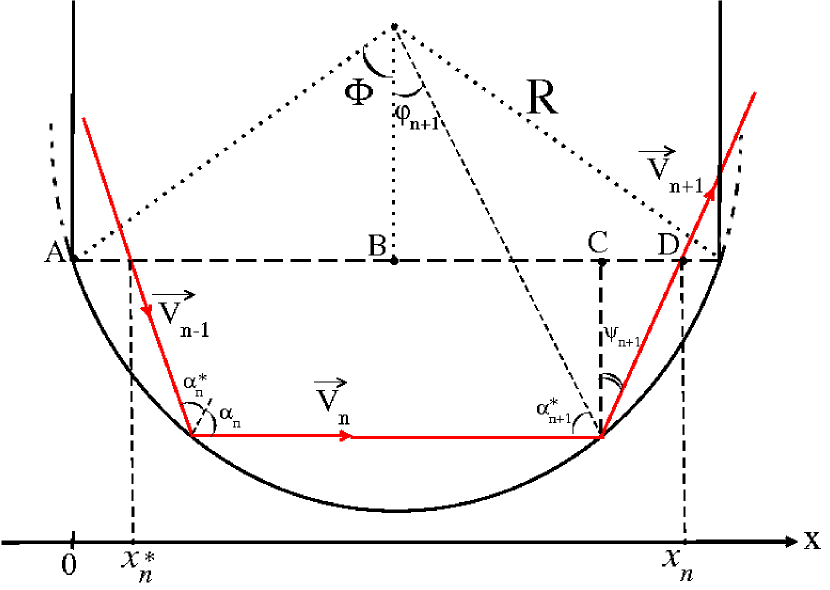
Figure 1: (color online) Dynamical variables and a typical trajectory with successive collisions.

shows an illustration of a trajectory with successive collisions, where $R=(a^{2}+4b^{2})/(8b)$ and $\Phi=\arcsin(a/2R)$. The control parameters $a$, $b$ and $l$ are drawn in Fig.2.

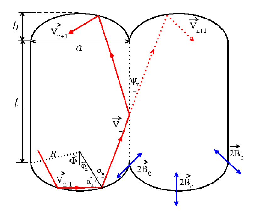
Figure 2: (color online) Illustration of the: (i) unfolding method; (ii) control parameters and (iii) a typical trajectory with indirect collisions with the focusing component.

If $a=2b$ the original stadium billiard is recovered.

Let us consider case (i) first. For the occurrence of a successive collision, it is necessary that $\mid\varphi_{n+1}\mid\leq\Phi$. Therefore, according to Fig. 1 and the specular reflection, we have that

$$\alpha^{*}_{n+1} = \alpha_{n}~{},$$

$$\varphi_{n+1} = \varphi_{n}+\pi-2\alpha_{n}~{}~{}(mod~{}2\pi)~{},$$

$$t_{n+1} = t_{n}+{2R\cos(\alpha_{n})\over V_{n}}~{}.$$

Considering the case of indirect collisions, case (ii), it is necessary that $\mid\varphi_{n+1}\mid>\Phi$. To obtain the equations describing the dynamics, it is useful to consider the unfolding method ref1 . Then two auxiliary variables, $\psi$, which is the angle between the trajectory and the vertical line at the collision point and, $x_{n}$, which is the projection of the particle position under the horizontal axis are used. From geometrical considerations of Fig. 1 we obtain that $\psi_{n}=\alpha_{n}-\varphi_{n}$. One sees also that $x_{n}$ is the summation of the line segments $\overline{AB}+\overline{BC}+\overline{CD}$. Taking into account the expression of $\psi_{n}$, and after some algebra, we obtain $x_{n}={R\over\cos(\psi_{n})}[\sin(\alpha_{n})+\sin(\Phi-\psi_{n})]$. The recurrence relation between $x_{n}$ and $x_{n+1}$ is given by the unfolding method, described in Fig. 2, as $x_{n+1}=x_{n}+l\tan(\psi_{n})$.

To obtain the angular equations, we invert the particle motion, i.e., consider the reverse direction of the billiard particle, then the expression that furnishes $x_{n}$ is also inverted and the angle $\alpha_{n}$ becomes $\alpha^{*}_{n}$. Resolving it with respect to $\alpha^{*}_{n}$, taking into account that this angle is changed in the opposite direction, then the angles $\alpha_{n}$ and $\varphi_{n}$ must have their sign reversed. Moreover, the incident angle $\alpha^{*}_{n}$ assumes $\alpha^{*}_{n+1}$ when the motion of the particle is re-inverted. The expressions of $\varphi_{n+1}$ and the time $t_{n+1}$ are obtained by simple geometrical considerations of Fig. 2. Thus, we obtain the mapping for the case of indirect collisions as

$$\alpha^{*}_{n+1} = \arcsin[\sin(\psi_{n}+\Phi)-x_{n+1}\cos(\psi_{n})/R]~{},$$

$$\varphi_{n+1} = \psi_{n}-\alpha^{*}_{n+1}~{},$$

$$t_{n+1} = t_{n}+{R[\cos(\varphi_{n})+\cos(\varphi_{n+1})-2\cos(\Phi)]+l\over V_{n}\cos(\psi_{n})}~{}.$$

For both cases (i) and (ii), the recurrence relations for $V_{n}$ and $\alpha_{n}$ are the same. Let us discuss how to obtain them. Expressing the two components of the velocity vector before the collisions we have that

$$\vec{V}_{n}\cdot\vec{T}_{n+1} = -V_{n}\cos(\alpha^{*}_{n})~{},$$

$$\vec{V}_{n}\cdot\vec{N}_{n+1} = V_{n}\sin(\alpha^{*}_{n})~{}.$$

Given that the moving boundary is not an inertial referential frame, we assume that at the instant of the collision, the wall is instantaneously at rest, then the reflection laws are given by

$$\vec{V}^{\prime}_{n+1}\cdot\vec{T}_{n+1} = \beta\vec{V}^{\prime}_{n}\cdot\vec{T}_{n+1}~{},$$

$$\vec{V}^{\prime}_{n+1}\cdot\vec{N}_{n+1} = -\gamma\vec{V}^{\prime}_{n}\cdot\vec{N}_{n+1}~{},$$

where $\beta$ and $\gamma$ are respectively the restitution coefficients with respect to the tangent and the normal components of the motion. We stress that $\vec{V}^{\prime}_{n+1}\cdot\vec{T}_{n+1}$ and $\vec{V}^{\prime}_{n+1}\cdot\vec{N}_{n+1}$ are the components of the velocity of the particle measured in the referential frame of the moving wall with respect to the tangent and the normal components respectively.

In the inertial referential frame, we have that the equations for the components of the velocity are given by

$$\vec{V}_{n+1}\cdot\vec{T}_{n+1}=\beta\vec{V}_{n}\cdot\vec{T}_{n+1}+(1-\beta)\vec{B}(t_{n+1})\cdot\vec{T}_{n+1}~{},$$

$$\vec{V}_{n+1}\cdot\vec{N}_{n+1}=-\gamma\vec{V}_{n}\cdot\vec{N}_{n+1}+(1+\gamma)\vec{B}(t_{n+1})\cdot\vec{N}_{n+1}~{},$$

where $B(t_{n+1})$ is obtained from Eq.(1) evaluated at the time $t_{n+1}$. Finally, the expression of $V_{n+1}$ is given by

$$\mid\vec{V}_{n+1}\mid=\sqrt{(\vec{V}_{n+1}\cdot\vec{T}_{n+1})^{2}+(\vec{V}_{n+1}\cdot\vec{N}_{n+1})^{2}}~{}.$$ (2)

The last equation refers to the reflection angle, which according to the reflection law is given by

$$\alpha_{n+1}=\arcsin\left({\mid\vec{V}_{n}\mid\over\mid\vec{V}_{n+1}\mid}\sin(\alpha^{*}_{n+1})\right)~{}.$$ (3)

III Discussions of the Dynamics and numerical results

To investigate the dynamics of the model, we set as fixed the parameters $a=0.5$, $b=0.01$, $l=1$ and the amplitude of oscillation of the moving wall as $B_{0}=0.01$. The reason for keeping the parameters fixed is because some observables are scaling invariant with respect to the control parameters, as discussed for the static case in Ref. liv . Therefore for this paper we chose to investigate the dynamics by the variation of the parameter $\gamma$ as well as the initial velocity $V_{0}$. The parameter $\beta$ is considered fixed as $\beta=1$. Moreover we stress that collisions of the particle with the straight segments of the border are considered elastic.

Figure 3 illustrates the dynamics of the particle on the variables $(\psi,\xi)$, where $\xi=x/a$, for the conservative case and the dissipative dynamics respectively. It is known from the literature that, when dissipation is introduced in the dynamics, the invariant curves surrounding the fixed points might be destroyed and the elliptic fixed points turn into sinks litch . Specific discussions of fixed points in the non dissipative case can be seen for the stadium-like billiard in Refs. losk1 ; losk2 ; losk3 ; liv . The procedure used to construct the phase portraits was to consider 25 different initial conditions and evolve each initial condition until $10^{7}$ collisions. For the conservative case, FA is indeed oberserved for the stadium billiard for an initial velocity higher than the critical resonant one losk1 , and the phase space for this unlimited energy growth is shown in Fig.3(a). On the other hand, the darker regions of Fig. 3(b) mark the convergence to the attractors while the spread points along the plot identify the seemingly chaotic transient. The control parameters and initial conditions used in the construction of the figure were: (a) $V_{0}=10$, $\gamma=1.0$ and (b) $V_{0}=10$, $\gamma=0.999$. Comparing Fig.3(a) and (b), one can see the “birth” of a period-2 atractor, and two period one atracting ponits.

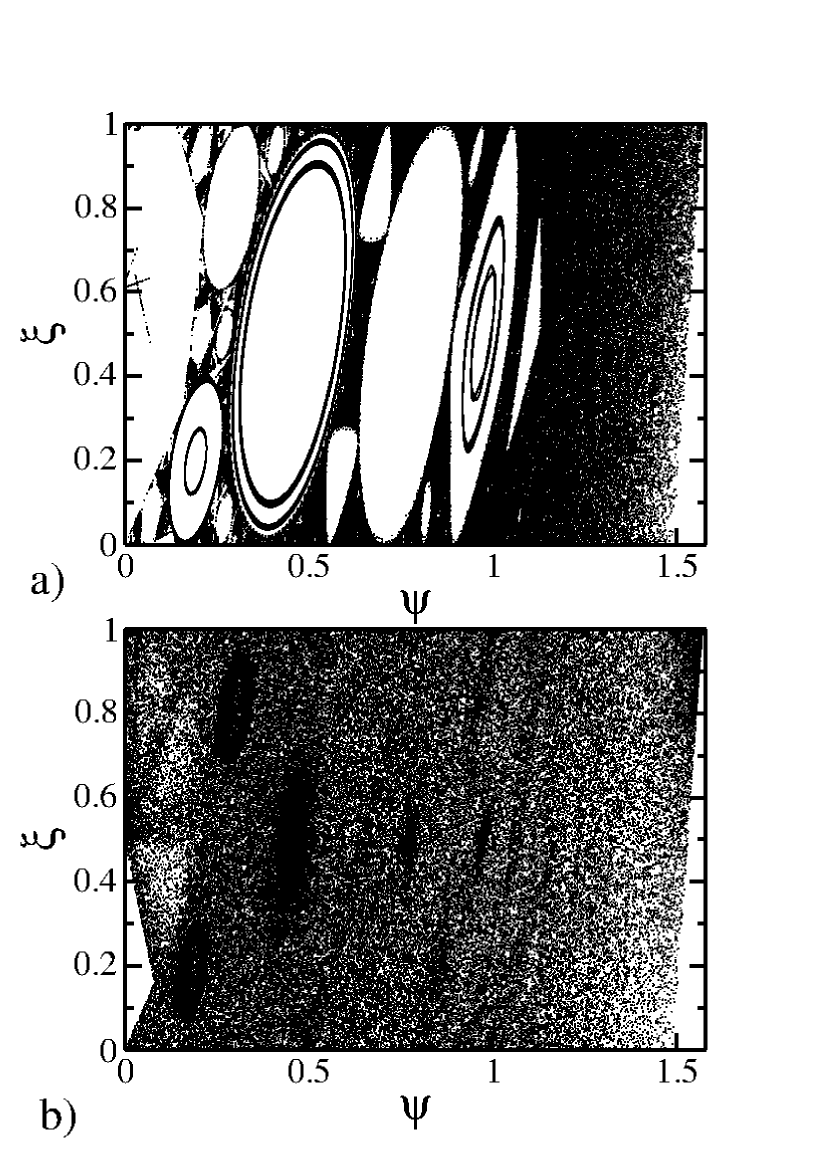
Figure 3: Phase portrait of $(\psi,\xi)$ for: (a) $V_{0}=10$, $\gamma=1.0$ and (b) $V_{0}=10$, $\gamma=0.999$.

In order to have a better understanding of the dynamics, particularly the convergence of the initial conditions to the attractors, we concentrate to study the dynamics and hence some properties of the average velocity of the particle. We consider dependence of the average velocity as function of both: (a) number of collisions with the boundary $n$; (b) initial velocity $V_{0}$ and; (c) restitution coefficient $\gamma$. The average velocity is therefore defined as

$$\overline{V}={1\over M}\sum_{j=1}^{M}{V_{i,j}(n,V_{0},\gamma)}~{},$$ (4)

where $M$ is an ensemble of $5000$ different initial conditions $(\alpha,\varphi)$, from which $\xi$ and $\psi$ are described, and $V_{i}$ is expressed by

$$V_{i}(n,V_{0},\gamma)={1\over n}\sum_{k=1}^{n}{V_{k}}~{},$$ (5)

where $n$ is the number of collisions with the moving wall.

The numerical investigations were carried out in two different ways. To understand the behavior of the average velocity and hence the energy of the particle at the range of large initial velocity we consider two regimes of time: (i) short time, mainly marked by the dynamics evolving through a transient and; (ii) long time where the dynamics has already reached the attractor. For high initial velocity, the particle experiences a decay in the average velocity marked by a transient in the dynamics. Moreover the decay of energy is described by a homogeneous function with critical exponents. (ii) For long time, a statistics is made to the regime of convergence ir order to understand the role of the dissipation and of the initial energy regime. The simulations were evolved up to $n=5\times 10^{8}$ collisions and considering an ensemble of $5000$ different initial configurations uniformly chosen as $\varphi\in[0,\Phi]$ and $\alpha\in[0,\pi/2]$. Due to the axial symmetry of the stadium-like billiard, a negative range of the initial conditions is not needed.

III.1 Transient for short time

In this section we concentrate to investigate the initial transient. Therefore we consider two ranges of initial velocity: (i) large and (ii) low. Let us start with the high energy. Figures 4(a,b) illustrate the behavior of $\overline{V}$ as function of the number of collisions. In Fig. 4(a) we assume as fixed the initial velocity as $V_{0}=100$, and varied the restitution coefficient $\gamma$. In Figure 4(b) we considered fixed $\gamma=0.999$ and varied the initial velocity $V_{0}$. The range of $V_{0}$ was chosen in such a way to configure a very large initial velocity as compared to the maximum boundary velocity $V_{0}>>r\omega$. The curves shown in Figs. 4(a) and 4(b) indeed exhibit similar behavior for short time. They begin in a constant regime for each initial velocity and suddenly, depending on the value of the damping coefficient $\gamma$, they experience a crossover $n_{x}$ marking a change from a constant regime and bend towards a regime of decay according a power law. A careful fitting in the curves gives that the decay exponent is $\zeta\approx-1$. After the decay observed for large $n$, the curves of $\overline{V}$ saturate in different plateaus of low energy, which may depend of both $V_{0}$ and $\gamma$. The plateaus characterize indeed different attractors to where the dynamics has converged to.

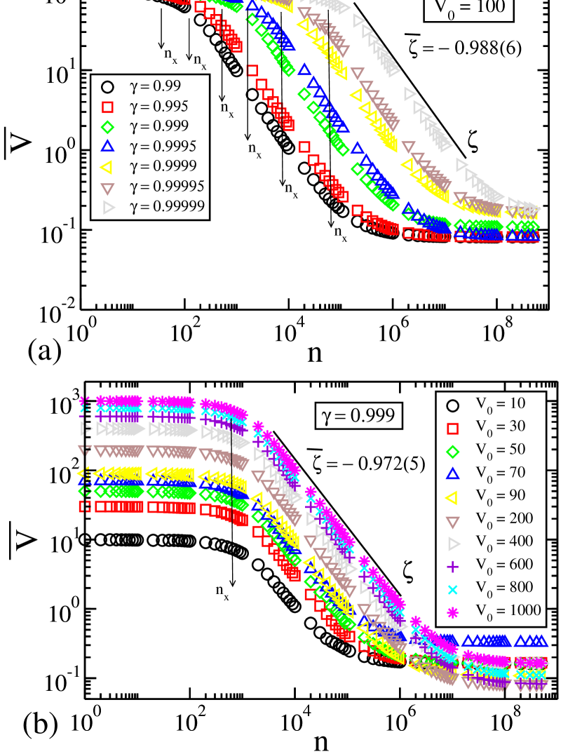
Figure 4: (color online) Plot of $\overline{V}~{}vs~{}n$ for the large initial velocity. The parameters and initial conditions used were: (a) $V_{0}=100$ and different restitution coefficients $\gamma$ and; (b) different initial velocities and a fixed $\gamma=0.999$.

For large enough time the convergence regions are around the range $V\in(0.07,0.6)$ The investigation of these plateaus will be made in the next subsection.

Given that the initial behavior of $\bar{V}$ for the range of large initial $V_{0}$ is similar even for different values of $V_{0}$ and $\gamma$, we can suppose that:

• (i) $\overline{V}\propto V_{0}^{\alpha}$, for $n\ll n_{x}$, where $\alpha$ is a critical exponent and $n_{x}$ is the characteristic crossover collision;

• (ii) $\overline{V}\propto\left({n\over V_{0}}\right)^{\zeta}$, for $n\gg n_{x}$, where $\zeta\approx-1$ is the power law decaying exponent;

• (iii) $\left({n_{x}\over V_{0}}\right)\propto V_{0}^{z_{1}}(1-\gamma)^{z_{2}}$, where $z_{1}$ and $z_{2}$ are dynamical exponents.

On the scaling hypothesis (iii) we considered $(1-\gamma)$ instead of $\gamma$, because we want to consider the transition $(1-\gamma)\rightarrow 0^{+}$. We see also that different initial velocities produce different curves of $\overline{V}$ but with the same negative slope. Therefore the transformation $n\rightarrow n/V_{0}$ makes all the curves coincide in the decay regime. This transformation together with some curves of $\overline{V}$ are shown in Fig. 5.

Figure 5: (color online) Plot of $\overline{V}$ as a function of: (a) $n$ and (b) $n/V_{0}$. The parameter $\gamma$ was fixed as $\gamma=0.999$ and 5 different initial conditions were used, as labeled in the figure.

After this transformation, all curves of $\overline{V}$ start in a constant regime and then decay together as a power law with exponent $\zeta\approx-1$.

Given that the initial behavior of $\overline{V}$ is constant, we conclude that $\alpha=1$. The critical exponents $z_{1}$ and $z_{2}$ are obtained respectively by power law fits on the plots $(n_{x}/V_{0})\times V_{0}$ and $(n_{x}/V_{0})\times(1-\gamma)$. Figure 6

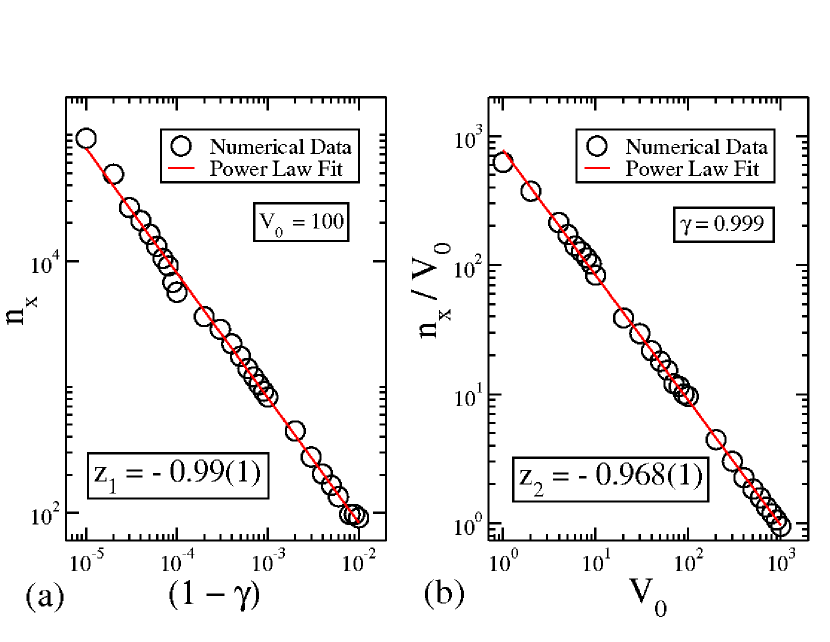
Figure 6: (color online) Plot of: (a) $n_{x}/V_{0}~{}vs~{}V_{0}$ for $\gamma=0.999$ and; (b) $n_{x}\times(1-\gamma)$ for $V_{0}=100$. After fitting the data we obtain $z_{1}=-0.99(1)$ and $z_{2}=-0.968(1)$.

gives us that $z_{1}=-0.99(1)$ and $z_{2}=-0.968(1)$.

The three scaling hypotheses allow us to describe the behavior of $\overline{V}$ for short $n$ (before the convergence to the constant plateau) formally as a scaling function of the type

$$\overline{V}(n/V_{0},V_{0}(1-\gamma))=\lambda\overline{V}(\lambda^{a_{1}}n/V_{0},\lambda^{b_{1}}V_{0}(1-\gamma))~{},$$ (6)

where $\lambda$ is a scaling factor and $a_{1}$ and $b_{1}$ are scaling exponents. Assuming that $\lambda^{a_{1}}n/V_{0}$ constant, we have

$$\lambda=\left({n\over V_{0}}\right)^{-{1\over a_{1}}}~{}.$$ (7)

Substituting Eq.(7) in (6), we obtain

$$\overline{V}(n/V_{0},V_{0}(1-\gamma))=V_{0}^{-{1\over a_{1}}}\overline{V_{1}}(1,\lambda^{-{b_{1}\over a_{1}}}V_{0}(1-\gamma))~{}.$$ (8)

If we compare Eq.(8) with the hypothesis (ii) and assuming that $\overline{V_{1}}$ is constant for $n\gg n_{x}$, we obtain

$$\zeta=-{1\over a_{1}}~{},$$ (9)

and given that the critical exponent $\zeta\approx-1$, obtained by fitting a power law to the decay regime, we have that $a_{1}=1$.

Choosing now $\lambda^{b_{1}}V_{0}(1-\gamma)$ constant, we have

$$\lambda=\left(V_{0}(1-\gamma)\right)^{-{1\over{b_{1}}}}~{}.$$ (10)

Replacing Eq.(10) in (6), we obtain

$$\overline{V}(n/V_{0},V_{0}(1-\gamma))=V_{0}(1-\gamma)^{-{1\over{b_{1}}}}\overline{V_{2}}(\lambda^{-{{a_{1}}\over{b_{1}}}}n/V_{0},1)~{}.$$ (11)

A comparison of Eq.(11) with hypothesis (i), and assuming $\overline{V_{2}}$ constant for $n\ll n_{x}$, leads to

$$\alpha=-{1\over b_{1}}~{},$$ (12)

and given the constancy of the initial regime, we conclude that $\alpha=1$, yielding $b_{1}=-1$.

Comparing now Eqs.(7) with (10) and after straightforward algebra, we obtain that

$$\left({n\over V_{0}}\right)=\left(V_{0}(1-\gamma)\right)^{{a_{1}\over b_{1}}}~{}.$$ (13)

When Eq. (13) is compared with the scaling hypothesis (iii) we conclude that

$${a_{1}\over b_{1}}={\alpha\over\zeta}=z_{1}=z_{2}=-1~{}.$$ (14)

This procedure and the critical exponents let us rescale properly both axis of the $\overline{V}~{}vs~{}n$ plot and obtain a single and universal curve for the short time transient dynamics, as shown in Fig. 7.

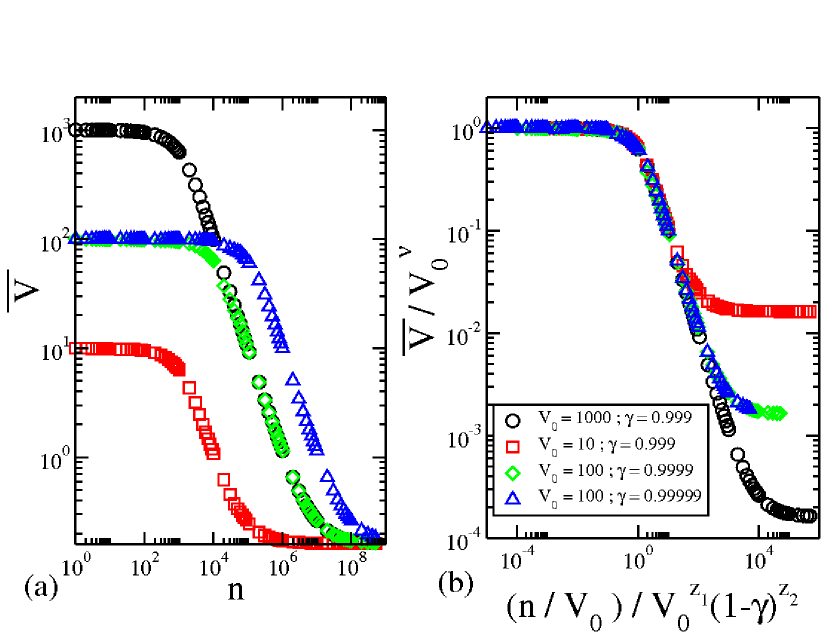
Figure 7: (color online) Plot of: (a) $\overline{V}~{}vs~{}n$, and (b) overlap of the initial transient of all curves of (a) onto a single plot, after a suitable rescale of the axis.

Basically, this result confirms that, independent of the initial velocity and the control parameter $\gamma\cong 1$, the behavior of the transient for the high energy regime of $\overline{V}$ curves is scaling invariant with respect to $V_{0}$ and $\gamma$.

Let us now consider the case where the initial velocity is low, therefore the behavior of the transient is different. The curves of $\bar{V}$ exhibit a regime of growth until they reach the convergence regions, as shows Figs. 8(a,b). The combination of control parameters $V_{0}$ was set in order to keep the initial velocity in the low energy regime. The dissipation and the initial velocity are labeled in the figure.

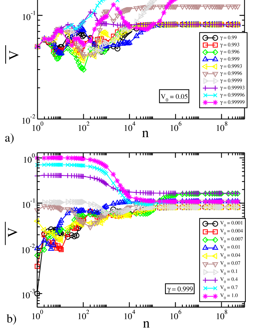
Figure 8: (color online) Plot of $\overline{V}~{}vs~{}n$ for the low energy regime: In (a) $V_{0}=0.05$ was fixed and the dissipation parameter $\gamma$ was ranged while; (b) $\gamma=0.999$ was fixed and the initial velocity for the a initial energy regime was ranged.

The presence of the attractors indeed define the region to where the curves of $\bar{V}$ converge to and therefore saturate. Although one may think this is quite a paradoxical behavior in the sense that dissipation leads to a regime of growth, if one looks deeper at the dynamics, indeed the particle is only converging to an attractor wich is located at higer energy compared to the initial velocity. Considering that this attractor is not at infinite velocity, the FA is suppressed.

III.2 Sinks, attractors and Convergence of $\overline{V}$

Once the behavior of the chaotic transient for both high and low energy regimes is described, let us concentrate our efforts to investigate the convergence regions, the role of the sinks and their dependence according the dissipation and initial velocities.

As shown in Fig. 3, the fixed points in the space $(\psi,\xi)$ become sinks. However a visualization of the phase portraits in such a variables does not give any conclusions regarding the final velocity. Then it is natural to look at the plots of $V$ vs $t~{}mod(2\pi)$ where $t$ is the time shown in Fig. 9.

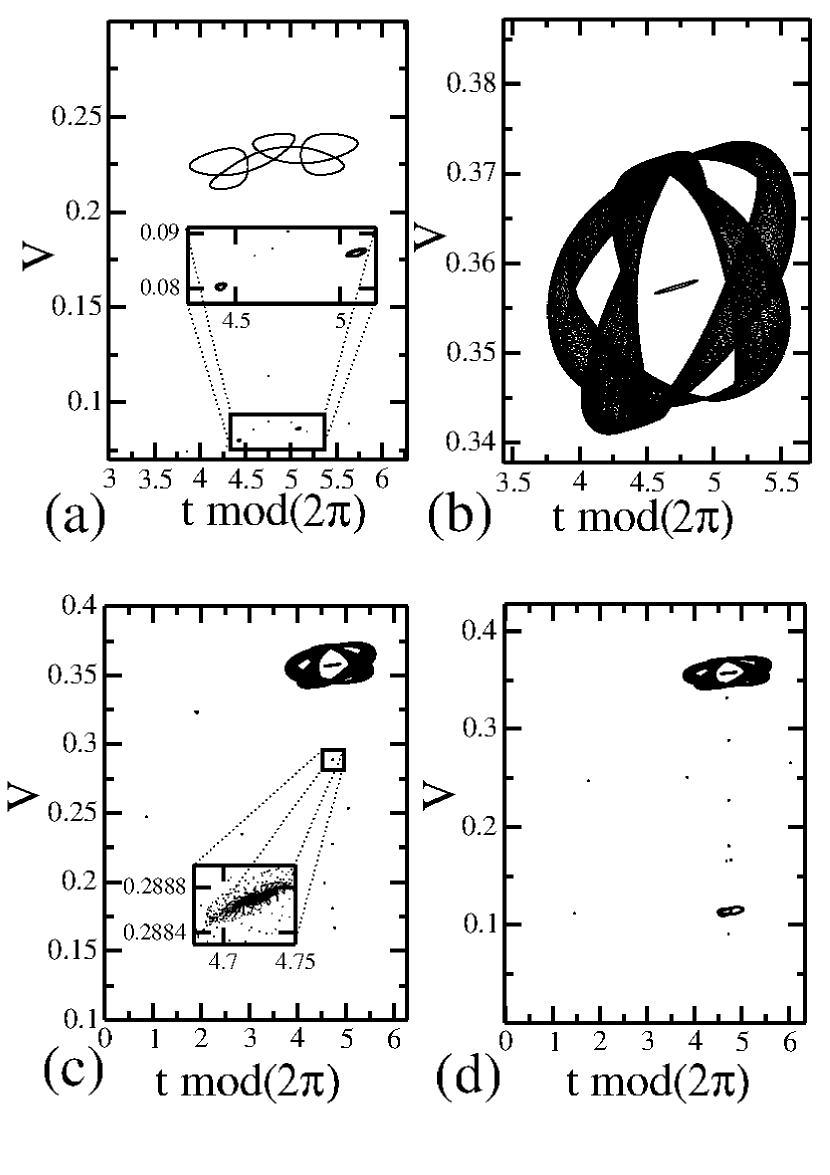
Figure 9: Plot of $V\times t~{}mod(2\pi)$ after the chaotic transient for: (a) $V_{0}=1000$, $\gamma=0.99$; (b) $V_{0}=100$, $\gamma=0.9999$; (c) $V_{0}=100$, $\gamma=0.999$ and (d) $V_{0}=10$, $\gamma=0.999$.

We can see that the convergence regions for the curves of $\overline{V}$ illustrated in Figs. 4 and 8 are around $V\in(0.07,0.6)$. It is also possible to see from Fig. 9 many different sets of attracting fixed points and more complex attractors. A zoom-in window shows better some of the sinks in Figs. 9(a,c). In particular, one can enumerate in Fig. 9(d) at least $13$ different attractors. Each attractor of this set produces a different plateau in the asymptotic curves of $\bar{V}$. This multitude of attracting points for the convergence zone is the reason why a scaling treatment for long time is indeed a real challenge. To construct the figures, we set $100$ different initial conditions, each one of them evolved in time until $5\times 10^{7}$ collisions.

Each attractor has its own influence over the dynamics which is dependent on the size of the basin of attraction. A way to see this is constructing a histogram of frequency of initial conditions showing convergence to a particular attractor. Figure 10 shows the corresponding histogram of frequency of visited attractors for the same control parameter used in Fig. 9 however with a large ensemble of initial conditions, indeed $25\times 10^{4}$ of them where each one of them was evolved until $5\times 10^{8}$ collisions.

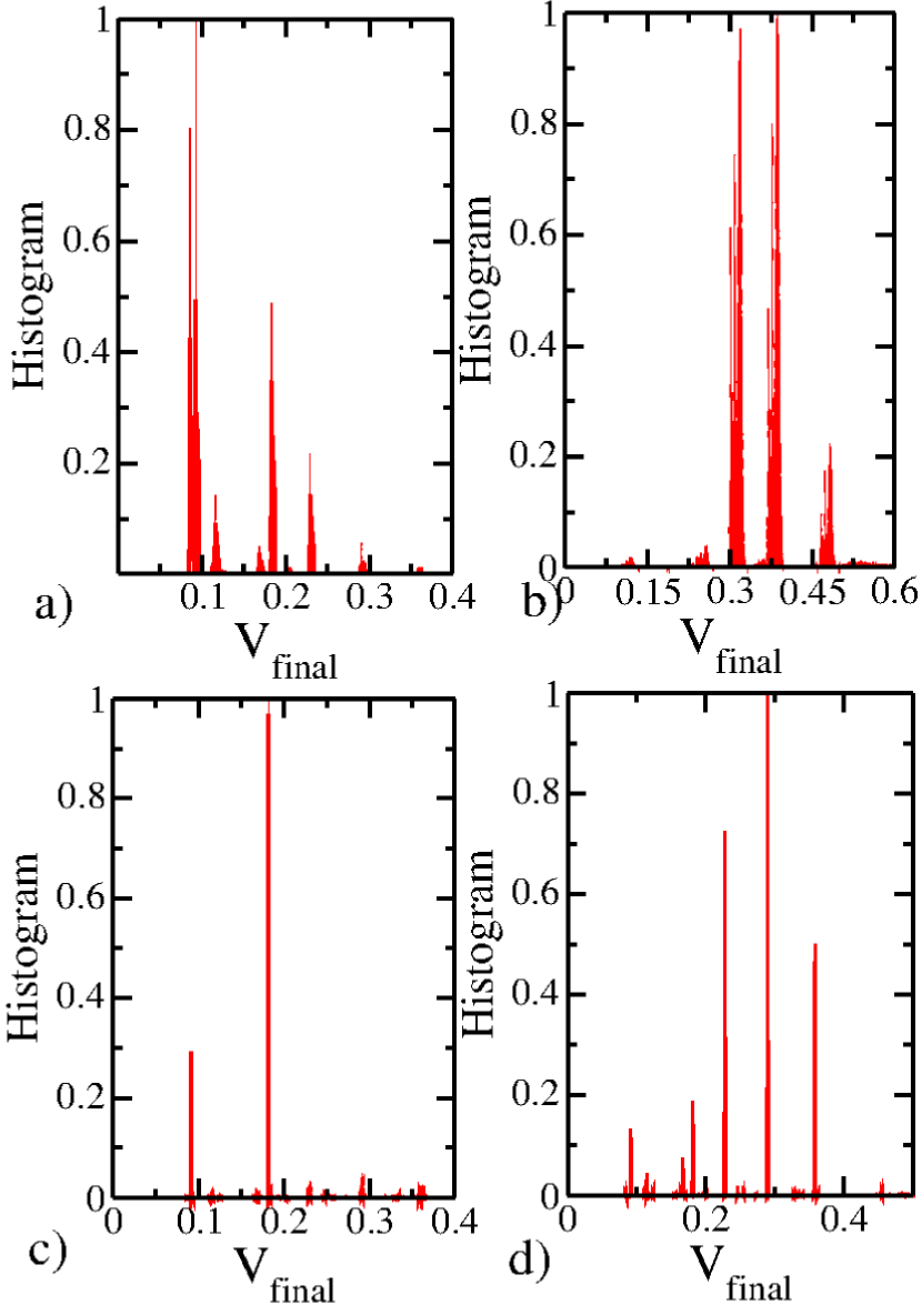
Figure 10: (color online) Histogram of frequency for the convergence velocity region for: (a) $V_{0}=1000$, $\gamma=0.99$; (b) $V_{0}=100$, $\gamma=0.9999$; (c) $V_{0}=100$, $\gamma=0.999$ and (d) $V_{0}=10$, $\gamma=0.999$.

Figure 10(a) shows that the most visited attractors are those located around $V\in(0.08,0.09)$. A comparison of this result with Fig. 9(a) shows one main attractor indicating a possibly period-2 attractor. Figure 10(b) shows that the distribution of final velocity of the orbits, for the combination of control parameters $\gamma=0.9999$ and $V_{0}=100$, are more concentrated in a range $V\in(0.3,0.4)$. Again, if the results are compared with Fig. 9(b), one sees that the visited region $V\in(0.3,0.4)$ corresponds to the seemingly cyclic attractor. Also, Figs. 10(c,d) show many different visited regions corresponding to the regions of final velocity as shown in Figs. 9(c,d).

The influence of the attractors are dependent on the control parameters used. Therefore specific attractors can be more influence than others for a combination of control parameters. In order to understand the dependence of the attractors with the dissipation parameter and the initial velocity, we constructed a histogram of frequency taking into account different control parameters and initial velocities, as shown in Fig. 11. After a careful look at Fig. 11, we conclude that the attractors for “more” dissipative systems, for example the ones for $\gamma\in[0.95,0.999]$, prefers the regions of lower velocities even considering the high and low initial velocity. On the other hand the “less” dissipative dynamics, for example for the range $\gamma\in[0.9995,0.999999]$, prefers regions of higher velocities as compared to the previous case. Each histogram shown in Fig. 11 was constructed considering $25\times 10^{4}$ different initial conditions where each one of them was evolved up to $5\times 10^{8}$ collisions. Figures 11(a,b) represent the histograms for the initial high velocity while Figs. 11(c,d) show the histograms for the low initial velocity. In particular, one can notice that in Fig. 11(d), the legend used for each parameter of dissipation $\gamma$, applies to all plots of Fig. 11.

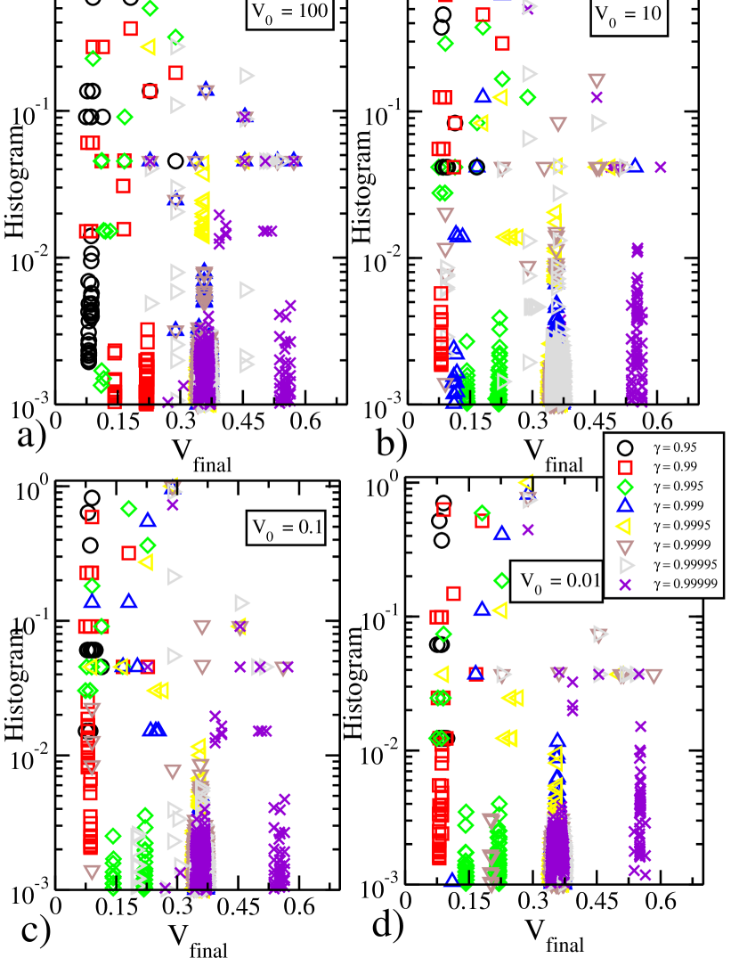
Figure 11: (color online) Histogram of frequency for different parameters $\gamma$. The control parameters and initial condition used were: (a) $V_{0}=100$, (b) $V_{0}=10$, (c) $V_{0}=0.1$ and (d) $V_{0}=0.01$.

IV Conclusions

In summary, we considered a time-dependent stadium-like billiard with dissipation introduced via inelastic collisions. With the introduction of the dissipation, we have shown that FA is suppressed. High initial velocities, after a crossover time, decay as a power law of the number of collisions with the border, while low initial energy regimes, lead the particle to present a regime of “growing” to the same convergence region of the orbits with a high energy chaotic transient. This chaotic transient for the high energy regimes, was characterized as function of both $V_{0}$ and $\gamma$. Scaling arguments were used to overlap the behavior of $\overline{V}$ for short $n$, showing that the dynamics of short time is scaling invariant with respect to $V_{0}$ and $\gamma$, if we considered high initial energy regime. The system is shown to have many attractors, where some of them are sinks and others are more complicate. When the damping coefficient is varied there is a tendency for more dissipation bringing the dynamics to visit more often the region $V_{final}\approx 0.30$. On the other hand, less dissipative dynamics prefers the attractors around $V_{final}\in(0.3,0.6)$. Finally, it is clear that the unlimited energy growth is interrupted with the presence of inelastic collisions therefore leading to one more example where Fermi acceleration seems not to be a structurally stable phenomenon.

References

- (1) N. Chernov and R. Markarian, Chaotic Billiards. (American Mathematical Society, Vol. 127, 2006).
- (2) G. D. Birkhoff, Dynamical Systems, (Am. Math. Soc. Colloquium Publ. vol 9) (Providence, RI: American Mathematical Society 1927).
- (3) Y. G. Sinai, Russ. Math. Surveys, 25, 137 (1970); 25, 141 (1970).
- (4) L. A. Bunimovich, Commun. Math. Phys., 65, 295 (1979).
- (5) L. A. Bunimovich and Y. G. Sinai, Commun. Math. Phys., 78, 479 (1981).
- (6) G. Gallavotti and D. S. Ornstein, Commun. Math. Phys., 38, 83 (1974).
- (7) N. Friedman et al., Phys. Rev. Lett., 86, 1518 (2001).
- (8) M. F. Andersen et al., Phys. Rev. A, 69, 63413 (2004).
- (9) M. F. Andersen et al., Phys. Rev. Lett., 97, 104102 (2006).
- (10) E. D. Leonel, Phys. Rev. Lett. 98, 114102 (2007).
- (11) H. J. Stokmann, Quantum Chaos: An Introduction. Cambridge University Press - 1999.
- (12) C. M. Marcus et al., Phys. Rev. Lett., 69, 506 (1992).
- (13) P. Fré, A. S. Sorin, J. High Energy Phys., 3, 1 (2010).
- (14) A. D. Stone, Nature, 465, 696 (2010).
- (15) E. Fermi. Phys. Rev., 75, 1169 (1949).
- (16) A. Loskutov, A. B. Ryabov and L. G. Akinshin, J. Phys. A, 33, 7973 (2000).
- (17) F. Lenz, F. K. Diakonos and P. Schemelcher, Phys. Rev. Lett., 100, 014103 (2008).
- (18) E. D. Leonel and L. Bunimovich, Phys. Rev. Lett., 104, 224101 (2010).
- (19) D. F. M. Oliveira and E. D. Leonel, Physica A, 389, 1009 (2010).
- (20) D. F. M. Oliveira, J. Vollmer and E. D. Leonel, Physica D, 240, 389 (2011).
- (21) E. D. Leonel and L. Bunimovich, Phys. Rev. E, 82, 016202 (2010).
- (22) D. F. M. Oliveira, M. Robnik, Phys. Rev. E, 83, 026202 (2011).
- (23) R. K. Pathria, Statistical Mechanics, Elsevier – Burlington 2008.
- (24) A. Loskutov and A. B. Ryabov, J. Stat. Phys., 108, 995 (2002).
- (25) A. Loskutov, A. B. Ryabov and E. D. Leonel, Physica A, 389, 5408 (2010).
- (26) A. B. Ryabov and A. Loskutov, J. Phys. A, 43, 125104 (2010).
- (27) E. D. Leonel, J. Phys. A: Math. Theor. 40, F1077 (2007).
- (28) A. L. P. Livorati, A. Loskutov and E. D. Leonel, J. Phys. A, 44, 175102 (2011).
- (29) A. J. Lichtenberg, M.A. Lieberman, Regular and Chaotic Dynamics. Appl. Math. Sci. 38, Springer Verlag, New York, 1992.