The Complex Energy Spectrum of Isomeric Reactions

Abstract

The internal motion in a molecule, in which isomerization processes occur, is characterized by two essentially different modes of motion - oscillatory and rotational. The quantum equation of motion which describes an isomerization process is reduced to the Mathieu-Hill equation. As is known, this equation is able to describe both modes. In the paper, it is shown that the chaotic region of the energy spectrum characterizing an isomerization process corresponds to the region where two modes of motion are merged together.

1 Introduction

Dynamic stochasticity [1, 2, 3] occurs in the region of parameter values, where topologically different trajectories adjoin each other. Trajectories near the boundary are highly sensitive to small disturbances. For small disturbances these trajectories take a very complicated shape, which is one of the manifestations of stochasticity.

An elementary example of such systems is a pendulum that may perform two kinds of motion - oscillatory and rotational. This explains in the main a growing interest in physical processes in which motion reduces to pendulum type motions.

A quantum analogue of dynamic stochasticity - quantum chaos [4, 5] occurs in the same region of parameter values where dynamic stochasticity does. In that case, the quantum states of two different symmetries adjoin each other. A highly complicated process takes place in a neighborhood of the boundary - the energy spectrum corresponding to the symmetry of one kind transforms to the energy spectrum of the other kind, which, in turn, demands the removal of degeneration corresponding to the symmetry of one kind and the appearance of degeneration corresponding to the symmetry of second kind. In the energy spectrum graph this process is represented by the set of branch points and merged energy levels. In passing through these points, the system may lose information on the initial conditions and pass from the pure state to the mixed one. The mixed state thus formed will be the state expressing quantum chaos. From that moment of time, the state of the system is not any longer described by a wave function and it becomes necessary to describe it by a density matrix [6, 7, 8].

Frequently, the objects of quantum chaos realization are polyatomic molecules [9, 10, 11, 12]. For example, quantum chaos may take place in a polyatomic molecule, one of the generalized coordinates of which performs torsional oscillations which, with an increase of the amplitude, transform to rotational motion [12]. Quantum chaos is a characteristic feature of such a transitional region.

From the standpoint of quantum chaos it is of special interest to investigate the so-called floppy molecules which have a capacity to isomerization [9, 10]. An example of such molecules is lithium cyanide (LiNC). This molecule contains a firm fragment $C\equiv N$ with a triple bond and a relatively light lithium atom (Li) which is able to perform angular oscillations relative to the molecule axis. When the oscillation amplitude attains the threshold value, the lithium atom detaches itself from the nitrogen atom and passes over to the carbon atom (Fig.1a). At higher energies, it again returns to the nitrogen atom and there begins the alternating jump-over process, i.e., the lithium atom begins to rotate about the fragment $C\equiv N$.

The energy spectrum of lithium atom motion was studied by the numerical methods in [9, 10]. It was shown that the energy spectrum consists of equidistant and nonequidistant regions. The energy levels arranged in a nonequidistant manner correspond to lithium atom states at which the oscillatory mode of motion transforms to the rotational one.

The aim of the present paper is to study the energy spectrum of lithium atom motion relative to the firm fragment $C\equiv N$. As different from the papers [9, 10], which are based mainly on the numerical methods, our approach to the problem is analytical: using numerical data we approximate the potential energy of the lithium atom and study the energy spectrum by the analysis of the Schrödinger equation.

2 An Isomerization Potential

The lithium atom motion relative to the firm fragment $C\equiv N$ can be described by means of two coordinates R and $\theta$ only (Fig.1b). $\theta=0^{0}$ and $\theta=180^{0}$ correspond to the equilibrium states of Li–CN and NC–Li, respectively. R is the distance between the lithium atom and the centre of mass of the fragment $C\equiv N$.

-

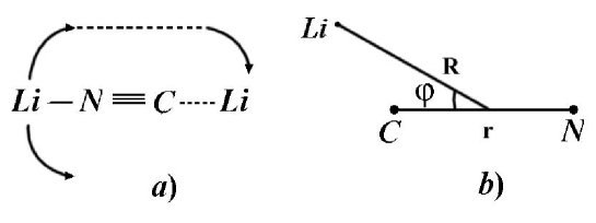
Figure 1: The izomerization reaction in lithium cyanide: a) lithium atom motion relative to the firm fragment; b) the coordinates R and $\theta$ describing the lithium atom.

The potential energy V of lithium atom motion relative to the firm fragment $C\equiv N$ was studied in [9] (Fig.2). It was shown that the potential energy has two different minima for $\theta=0^{0}$ and $\theta=180^{0}$. The energy distance between these minima is $\emph{V}(180^{0})-\emph{V}(0)\approx 6.21$ kcal/mol,while the distance from the minimum at $\theta=0^{0}$ to the maximum is 3.42 kcal/mol. Totally, the isomerization energy, i.e. the distance from $\emph{V}(180^{0})$ to $\emph{V}_{max}$ is $\approx 9.63$ kcal/mol (Fig.2).

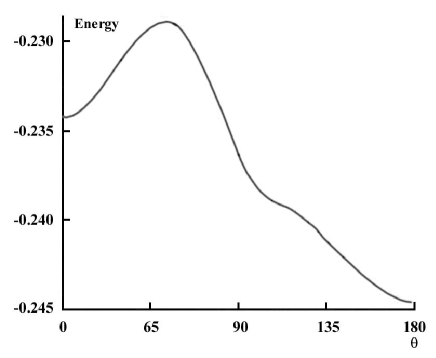
Figure 2: The plot of the potential energy $\emph{V}(\theta)$ obtained by a numerical method [9]. The angle $\theta$ is laid off along the abscissa axis, and the potential energy in atom units $(1\ am.u.=627.52\ kcal/mol,1\ kcal/mol=7\cdot 10^{-21}J)$ is laid off along the ordinate axis.

It can be easily verified that the potential energy of isomerization is approximated by the formula

$$V(\theta)=C+\alpha_{1}\cos\theta-\alpha_{2}cos^{2}\theta,$$

where $\alpha_{1}<2\alpha_{2}$. Indeed, the points of a minimum of the potential energy $V(\theta)$ are $\theta=\pi{n}$, while the points of a maximum $\theta_{\pm}=\pm\arccos\frac{\alpha_{1}}{2\alpha_{2}}+2\pi{n}$. If $\alpha_{1}\rightarrow 2\alpha_{2}$, then $\theta_{+}\rightarrow\theta_{-}\rightarrow 2\pi{n}$. This means that minima vanish at points $2\pi{n}$, while maxima adjacent to them merge. Therefore $\alpha_{1}<2\alpha_{2}$ is the condition of existence of two pits with different depth values.

We begin the reading of the potential energy $\emph{V}(\theta)$ from the largest minimum $\emph{V}[(2n+1)\pi]$. Then $C=\alpha_{1}+\alpha_{2}$, and for defining the numerical values of $\alpha_{1}$ and $\alpha_{2}$ we obtain the equations $\emph{V}(\theta)=2\alpha_{1}$, $\emph{V}(\pi)=0$, $\emph{V}_{max}=\emph{V}(\theta_{\pm})=\frac{(2\alpha_{2}+\alpha_{1})^{2}}{4\alpha_{2}^{2}},$ from which for the above-mentioned numerical values we obtain $\alpha=3.245$ kcal/mol and $\alpha_{2}=6.243$ kcal/mol.

The plot of the approximated potential energy is shown in Fig.3. It should be noted that the existence of potential minima of different heights is typical of isomerization processes where the firm fragment is nonsymmetric [13].

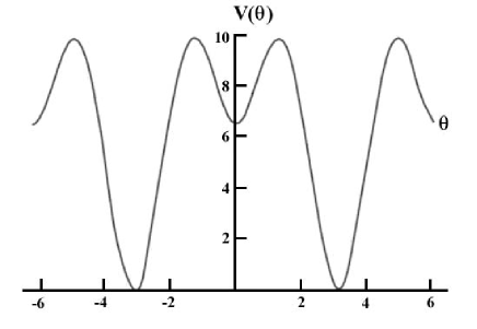
Figure 3: The potential energy of the lithium atom representing the isomerization process. The graph is constructed for the potential energy $V(\theta)=\alpha_{2}+\alpha_{1}+\alpha_{1}\cos\theta-\alpha_{2}\cos^{2}\theta,$ when $\alpha_{1}<2\alpha_{2}$.

A Hamiltonian function describing the lithium atom motion relative to the firm fragment $C\equiv N$ has the form

$$H=\frac{P^{2}_{\theta}}{2I}+V(\theta),$$ (1)

where $I=M_{1}R^{2}+M_{2}r^{2}$ is the moment of inertia, and $P_{\theta}$ is the generalized pulse corresponding to the cyclic variable $\theta$.

$$\frac{1}{M_{1}}=\frac{1}{m_{Li}}+\frac{1}{m_{N}+m_{C}},\qquad\frac{1}{M_{2}}=\frac{1}{m_{N}}+\frac{1}{m_{C}},$$ (2)

$$V(\theta)=\alpha_{2}+\alpha_{1}+\alpha_{1}\cos\theta-\alpha_{2}\cos^{2}\theta.$$ (3)

$m_{Li}$, $m_{N}$ and $m_{C}$ are the masses of lithium, nitrogen and carbon atoms. The expression (1) does not take into account the radial motion of the lithium atom, which is assumed to be at some average distance from the fragment $C\equiv N$.

3 The Classical Consideration. The Phase Portrait

Let us first consider the lithium atom motion relative to the firm fragment $C\equiv N$ in classical terms. For the sake of simplicity, we will study this motion for energy $E>2\alpha$. As will be seen later, these energy values include the oscillation and rotation modes which we are interested in.

To obtain the motion equation, we write the energy integral

$$\frac{I\dot{\theta}^{2}}{2}+\alpha_{1}+\alpha_{2}+\alpha_{1}\cos\theta-\alpha_{2}\cos^{2}\theta=E.$$ (4)

Using this integral of motion we can obtain a period of the lithium atom rotation about the fragment $C\equiv N$

$$T_{+}=2\sqrt{\frac{I}{2}}\int\limits_{0}^{\pi}\frac{d\theta}{\sqrt{E-U(\theta)}}=2\sqrt{\frac{I}{2}}\sum_{\pm}F(\gamma_{\pm},r),$$

where

$$\gamma_{\pm}=\arcsin\left(\left(1\pm\frac{\alpha_{1}}{2\alpha_{2}}\right)\sqrt{\frac{a^{2}+1}{a^{2}+\left(1\pm\frac{\alpha_{1}}{2\alpha_{2}}\right)^{2}}}\right),\qquad a^{2}=\frac{E}{\alpha_{2}}-\left(1+\frac{\alpha_{1}}{2\alpha_{2}}\right)^{2},$$

$$r=\sqrt{\frac{(1-b)(c+1)}{(1-c)(b+1)}},\qquad b=\frac{\alpha_{1}}{2\alpha_{2}}+\sqrt{\left(1+\frac{\alpha_{1}}{2\alpha_{2}}\right)^{2}-\frac{E}{\alpha_{2}}},$$

$$c=\frac{\alpha_{1}}{2\alpha_{2}}-\sqrt{\left(1+\frac{\alpha_{1}}{2\alpha_{2}}\right)^{2}-\frac{E}{\alpha_{2}}}.$$

Here

$$F(\alpha,k)=\int_{0}^{\alpha}\frac{d\varphi}{\sqrt{1-k^{2}\sin^{2}\varphi}}$$

is a eliptic function of first order.

When $E\rightarrow+E_{c}=\frac{\left(2\alpha_{2}+\alpha_{1}\right)^{2}}{4\alpha_{2}},$ in the limit from above we have $a\rightarrow 0$, $\gamma_{\pm}\rightarrow\frac{\pi}{2}$, $r\rightarrow 1$, and the rotation period

$$T_{+}\rightarrow+T_{c}=4\sqrt{\frac{I}{2\alpha_{2}}}F\left(\frac{\pi}{2},r\rightarrow 1\right)=4\sqrt{\frac{I}{2\alpha_{2}}}\ln\frac{4}{\sqrt{1-r^{2}}}\rightarrow\infty.$$

Therefore as $E\rightarrow+E_{c}$ the rotation period logarithmically tends to infinity. Analogosously, we can calculate the oscillatory motion period $T_{-}$. These calculations are not given here. We only note the oscillatory motion period, too, diverges logarithmically when $E\rightarrow-E_{c}$, i.e., if $E\rightarrow-E_{c}$, then $T_{-}\rightarrow-T_{c}\rightarrow\infty$.

As a rule, the existence of a logarithmically diverging period indicates the presence of two different modes of motion and the existence of a boundary trajectory - separatrix between them. This means that the separatrix appears to be obtained at energies $E=-E_{c}$.

Using the expression (4) we can construct the phase portrait on the plane $(\dot{\theta},\theta)$. As seen from Fig.4, the phase portrait consists of closed (elliptic) trajectories, which correspond to the oscillatory process, and wave trajectories describing rotational motion. The alternation of elliptic trajectories of two different dimensions on the $\theta$-axis is caused by the presence of two different minima of potential energy. Thus we see that lithium atoms may have two types of motion - oscillatory when $E<\frac{(2\alpha_{2}+\alpha_{1})^{2}}{4\alpha_{2}}$ and rotatory when $E>\frac{(2\alpha_{2}+\alpha_{1})^{2}}{4\alpha_{2}}$. As seen from the figure these two types of motion are divided by the separatrix.

-

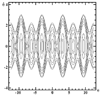
Figure 4: The phase portrait corresponding to an isomerization process, constructed by means of the equation (4).

4 Quantum-Mechanical Consideration of Motion. The Mathieu-Hill- Schrödinger Equation.

Let us now consider the motion of the lithium atom relative to the fragment $C\equiv N$ from the standpoint of quantum mechanics. We replace the Hamiltonian function (1) by the Hamilton operator

$$\hat{H}=\frac{\hat{p}^{2}}{2I}+V(\theta),$$ (5)

where $\hat{p}=-i\hbar\frac{\partial}{\partial\theta}$ is a pulse operator. Then the Schrödinger equation takes the form

$$-\frac{\hbar^{2}}{2I}\frac{\partial^{2}\psi}{\partial\theta^{2}}+(\alpha_{1}+\alpha_{2}+\alpha_{1}\cos\theta-\alpha_{2}\cos^{2}\theta)\psi=\varepsilon\psi.$$ (6)

We make the replacement $\theta\rightarrow 2\theta$ and introduce the notation

$$E=\frac{8I}{\hbar^{2}}\left(\epsilon-\alpha_{1}-\alpha_{2}+\frac{\alpha_{2}}{2}\right),\qquad q_{1}=\frac{8I}{\hbar^{2}}\alpha_{1},\qquad q_{2}=-\frac{8I}{2\hbar^{2}}\alpha_{2}.$$

Then, by simple transformations, from the equation (6) we obtain

$$\frac{d^{2}\psi}{d\theta^{2}}+\left[E-2\lambda(q_{1}\cos 2\theta+q_{2}\cos 4\theta\right)]\psi=0.$$ (7)

For the sake of simplicity, we restrict our consideration to the investigation of the dependence of energy levels on one (and not on two) parameter and to this end we introduce the parameter $\lambda$ into (7). This relationship is studied assuming $q_{1}$ and $q_{2}$ to be given values. The energy spectrum of the initial problem is obtained at $\lambda=0.5$. The Schrödinger equation takes the form known as the Hill equation which in turn implies the Mathieu equation as $q_{1}\rightarrow 0$. Using the known methods [14], solutions of this equation are sought for in the form of Fourier series

$$Ce_{2n}(z;\lambda;q_{1},q_{2}) = \sum_{r=0}^{\infty}A_{2r}^{(2n)}(\lambda)\cos{2rz},$$

$$Ce_{2n+1}(z;\lambda;q_{1},q_{2}) = \sum_{r=0}^{\infty}A_{2r+1}^{(2n+1)}(\lambda)\cos(2r+1)z.$$

$$Se_{2n+1}(z;\lambda;q_{1},q_{2}) = \sum_{r=0}^{\infty}B_{2r+1}^{(2n+1)}(\lambda)\sin(2r+1)z,$$

$$Se_{2n+2}(z;\lambda;q_{1},q_{2}) = \sum_{r=0}^{\infty}B_{2r+2}^{(2n+2)}(\lambda)\sin(2r+2)z.$$ (8)

Substituting these values into the equation (7) and equating the coefficients of the same harmonic, we obtain recurrent relations for the coefficients $A_{2r}$, $A_{2r+1}$, $B_{2r}$, $B_{2r+1}$, (their upper indexes are omitted). For example, for the first series of (8) these relations have the form:

$$r = 0\qquad aA_{0}-\lambda{q_{1}A_{2}}-\lambda{q_{2}A_{4}}=0,$$

$$r = 1\qquad(a-4)A_{2}-2\lambda{q_{1}A_{0}}-\lambda{q_{1}A_{4}}-\lambda{q_{2}A_{2}}-\lambda{q_{2}A_{6}}=0,$$

$$r = 2\qquad(a-16)A_{4}-\lambda{q_{1}A_{2}}-\lambda{q_{1}A_{6}-2}\lambda{q_{2}A_{0}}-\lambda{q_{2}A_{8}}=0,$$

$$r = 3\qquad(a-36)A_{6}-\lambda{q_{1}A_{4}}-\lambda{q_{1}A_{8}}-\lambda{q_{2}A_{2}}-\lambda{q_{2}A_{10}}=0,$$

$$r \geq 4\qquad(a-4r^{2})A_{2r}-\lambda{q_{1}A_{2(r-1)}}-\lambda{q_{1}A_{2(r+1)}}-\lambda{q_{2}A_{2(r-2)}}-$$ (9)

$$-\lambda{q_{2}A_{2(r+2)}}=0.$$

This is an infinite system of equations that establishes a relation between the coefficients $A_{2r}$. In order that this system would have a nontrivial solution it is necessary that $Det(A_{ij})=0$, where

$$A_{ij} = \left[a-4(i-1)^{2}\right]\delta_{ij}-\lambda{q_{1}\delta_{i+1;j}}-\lambda{q_{2}\delta_{i+2;j}}-\lambda{q_{1}\delta_{i;j+1}}-\lambda{q_{2}\delta_{i;j+2}}-$$ (10)

$$-\lambda{q_{1}\delta_{i;2}\delta_{j;1}}-\lambda{q_{2}\delta_{i;3}\delta_{j;1}}-\lambda{q_{2}\delta_{i;2}\delta_{j;2}},\ i=1\ldots\infty,\ j=1\ldots\infty.$$

are elements of the matrix composed of the coefficients of the system of equations (9) and written by means of the Kronecker symbol. Analogously, we obtain recurrent relations for the coefficients $A_{2r+1}$, $B_{2r}$ and $B_{2r+1}$, matrix determinants and characteristic equations, the numerical solution of which gives the energy spectrum.

5 A Quantitative Estimate of an Energy Spectrum

To obtain a quantitative estimate of the energy spectrum, we have to calculate first the numerical values of the parameters $q_{1}$ and $q_{2}$ contained in the Mathieu-Hill equation (7).

Applying the obtained values of $\alpha_{1}$ and $\alpha_{2}$, taking into consideration the carbon, nitrogen and lithium mass values ($m_{C}=19.92\cdot 10^{-27}kg,$ $m_{N}=23.24\cdot 10^{-27}kg,$ $m_{Li}=11.62\cdot 10^{-27}kg$) and also the values of the linear parameters r and R from [9] ($r=2.186a_{0}=11.57\cdot 10^{-11}m,$  $R=4.05a_{0}=21.43\cdot 10^{-11}m,$), we obtain, by means of the equations (2),$q_{1}=\frac{8I}{\hbar^{2}}\alpha_{1}\approx 9300$ and $q_{2}=-\frac{8I}{\hbar^{2}}\alpha_{2}\approx-8942$. Using the obtained values of $q_{1}$ and $q_{2}$ and the numerical solutions of the characteristic equation, we can construct the energy spectrum as a function of Mathieu characteristics $E(\lambda)$ (Fig.5).

As seen from Fig.5a, for low energies we have levels arranged equidistantly, which corresponds to oscillations of the lithium atom near the nitrogen molecule, i.e., to oscillatory motion in a deep ($\theta=0^{0}$) pit (Fig.3). When the lithium atom energy is $\varepsilon\geq 6\mbox{\ kcal/mol}$, the alternating transition from one pit to the other and vice versa takes place. In Fig.5 to this transition there correspond levels arranged nonequidistantly. The spectrum obtained by us qualitatively coincides with the picture obtained in [10]. In both cases nonequidistant levels appear in the same intervals of energy.

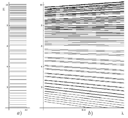
Figure 5: The spectrum of lithium atom motion about the fragment $C\equiv N$. Spectrum given in the Fig.5a is obtained from the Fig.5b by means of projection on the energetic axis of the values of energy at $\lambda=0.5$. a) we see the nonequidistance of energy levels of the lithium atom at energies $\varepsilon\geq 6\mbox{\ kcal/mol}$. In this region, the transition from the oscillatory mode to the rotational one takes place. b) the energy spectrum depending on the parameter $\lambda$.

6 Conclusion

Finding of energy spectrum of states which corresponds to the process of isomerization comes to the finding of proper values of Mathieu-Hill equation.

The energy spectrum of lithium atom motion includes a region $\varepsilon<4kcal/mol$, where levels are arranged equidistantly. These levels correspond to small oscillations of the lithium atom near isomeric states. Levels arranged nonequidistantly begin for relatively high energies, when the energy level reaches half of the barrier height and exceeds $\varepsilon\geq 6kcal/mol$.

It should be noted that the system considered in the paper is integrable. Therefore the generality of nonequidistant (chaotic) levels is not the manifestation of quantum chaos though it may appear when these states are disturbed by periodic force as illustrated by the example of a quantum pendulum [7, 8].

Acknowledgement

The financial support by the Deutsche Forschungsgemeinschaft (DFG) through SFB 762, grant No. KO-2235/3 and STCU grant No 5053 is gratefully acknowledged.

References

- [1] A.J. Lichtenberg and M.A. Liberman. Regular and Stochastic Motion. Springer-Verlag, New York, 1983.
- [2] R.Z. Sagdeev, D. A. Usikov and G.M. Zaslavsky. Nonlinear Physics. Hardwood, Acad. Publ.New York,1988.
- [3] K.T. Alligood, T.D. Sauer, J. York. Chaos and Introduction to Dynamical Systems.Springer, New York, 1996.
- [4] H.J. Stockmann. Quantum Chaos. An Introduction. Cambridge Univ. Press,Cambridge, 1993.
- [5] F. Haake. Quantum Signatures of Chaos. Springer, Berlin, 2001.
- [6] L.Chotorlishvili, A.Ugulava Physica D. 239, (2010), 103.
- [7] A.Ugulava, L.Chotorlishvili and K. Nickoladze. Phys. Rev. E70, (2004), 026219.
- [8] A.Ugulava, L.Chotorlishvili and K. Nickoladze. Phys. Rev. E71, (2005), 056211.
- [9] R.Essers, J. Tennyson and P.E.S. Wormer, Chemical Physics Letters. 89, No.3, (1982), 223.
- [10] F.J. Arranz, F. Borondo, R.M. Benito. Eur. Phys. J. Ser. D, 4, (1998), 181.
- [11] V.V. Eryomin, I.M. Umanskii, N.E. Kuz’menko. Chem. Phys. Lett. 316, No.3-4, (2000), 303.
- [12] A. Ugulava, L.Chotorlishvili, T. Gvardgaladze and S. Chkhaidze. Modern Physics Letters, 21, No.7, (2007), 415.
- [13] G. Herzberg, Infrared and Raman Spectra of Polyatomic Molecules, New-York, 1945.
- [14] N.W. McLachlan. Theory and Application of Mathieu Functions. Oxford, 1947.