Steady state fluctuation relation and time-reversibility for non-smooth chaotic maps

Abstract

Steady state fluctuation relations for dynamical systems are commonly derived under the assumption of some form of time-reversibility and of chaos. There are, however, cases in which they are observed to hold even if the usual notion of time reversal invariance is violated, e.g. for local fluctuations of Navier-Stokes systems. Here we construct and study analytically a simple non-smooth map in which the standard steady state fluctuation relation is valid, although the model violates the Anosov property of chaotic dynamical systems. Particularly, the time reversal operation is performed by a discontinuous involution, and the invariant measure is also discontinuous along the unstable manifolds. This further indicates that the validity of fluctuation relations for dynamical systems does not rely on particularly elaborate conditions, usually violated by systems of interest in physics. Indeed, even an irreversible map is proved to verify the steady state fluctuation relation.

1 Introduction

One of the central aims of nonequilibrium statistical physics is to find a unifying principle in the description of nonequilibrium phenomena. Nonequilibrium fluctuations are expected to play a major role in this endeavor, since they are ubiquitous, are observable in small as well as in large systems, and a theory about them is gradually unfolding, cf. Refs. [24, 11, 16, 9, 1, 3] for recent reviews. A number of works have been devoted to the derivation and test of fluctuation relations (FRs), of different nature [18, 19, 28, 31, 42, 2, 4, 34]. It is commonly believed that, although nonequilibrium phenomena concern a broad spectrum of seemingly unrelated problems, such as hydrodynamics and turbulence, biology, atmospheric physics, granular matter, nanotechnology, gravitational waves detection, etc. [1, 5, 6, 7], the theory underlying FRs rests on deeper grounds, common to the different fields of application. This view is supported by the finding that deterministic dynamics and stochastic processes of appropriate form obey apparently analogous FRs [1, 3, 42, 2], and by the fact that tests of these FRs on systems which do not satisfy all the requirements of the corresponding proofs typically confirm their validity. Various works have been devoted to identify the minimal mathematical ingredients as well as the physical mechanisms underlying the validity of FRs [29, 4, 30, 3]. This way, the different nature of some of these, apparently identical but different, FRs has been clarified to a good extent [4, 16, 2, 3]. However, analytically tractable examples are needed to clearly delimit the range of validity of FRs, and to further clarify their meaning.

In this paper, the assumptions of time reversal invariance and of smoothness properties, required by certain derivations of FRs for deterministic dynamical systems, are investigated by means of simple models that are amenable to detailed mathematical analysis. In particular, we consider the steady state FR for the observable known as the phase space contraction rate $\Lambda$, which we call the $\Lambda$-FR, for dissipative and reversible dynamical systems, in cases in which $\Lambda$ equals the so-called dissipation function $\Omega$ [24], and the $\Lambda$-FR then equals the steady state $\Omega$-FR [4]. As will be shown below, the phase variables $\Lambda$ and $\Omega$ coincide provided that the probability density entering the definition of $\Omega$ is taken uniform, as in the case of the equilibrium density for the baker map [25]. Both the $\Lambda$-FR and the $\Omega$-FR rest on dynamical assumptions: While the steady state $\Omega$-FR has been proven to hold under the quite mild condition of decay of correlations with respect to the initial (absolutely continuous, with respect to the Lebesgue measure) phase space distribution [4], the $\Lambda$-FR has been proven for a special class of smooth, hyperbolic (Anosov) dynamical systems [18, 19], whose natural measure is an SRB measure. Indeed, there are almost no systems of physical interest that strictly obey such conditions. However, in a similar fashion, there are almost no systems of physical interest satisfying the Ergodic Hypothesis, and yet this hypothesis is commonly adopted and leads to correct predictions. Analogously to the ergodic condition, one may thus interpret the Anosov assumption as a practical tool to infer the physical properties of nonequilibrium systems. Nevertheless, it is important to investigate which aspects of the derivation of the $\Lambda$-FR are not essential to its validity. Along these lines one notices that the $\Lambda$-FR seems to inherently rely on a rigid notion of time reversibility, which, however, is not always satisfied [17], and on the smoothness of the natural measure along the unstable directions, which is also problematic. On the other hand, the validity of the $\Omega$-FR has never been explicitly checked on an exactly solvable model.

By considering a fundamental class of chaotic dynamical systems, known as baker maps, we want to assess the relevance of the Anosov assumption and of time reversibility for the validity of the $\Lambda$-FR, in cases in which it coincides with the $\Omega$-FR. Also, by assessing the validity of these FRs while violating standard assumptions, we probe and extend their range of validity. The maps we consider are appealing, since they are among the very few dynamical systems which can be analytically investigated in full detail. For this reason, baker maps have often been used as paradigmatic models of systems that enjoy nonequilibrium steady states (NESS) [25, 12, 9, 35, 36].

Our main results are summarized as follows: The assumed sufficient conditions of the standard derivation of the $\Lambda$-FR, i.e. smooth time reversal operator and the Anosov property, are not necessary. Indeed, the $\Lambda$-FR is verified in maps whose invariant measure and time reversal involution are discontinuous along the unstable direction. This result is connected with the fact that $\Lambda$ equals $\Omega$, and that the $\Omega$-FR is known to be quite a generic property of reversible dynamics. The Anosov condition allows the natural measure to be approximated in terms of unstable periodic orbits, which constitutes a convenient tool in low dimensional dynamics and even in some high dimensional cases [14, 11, 32, 5]. This approximation may hold even if the Anosov condition is not strictly verified, because periodic orbits enjoy particular symmetries which other trajectories do not [15]. However, if the Anosov condition is violated, one must check case by case whether the unstable periodic orbit expansion may be trusted. We will also face this issue, showing that in some case the unstable periodic orbit expansion becomes problematic, hence a different approach must be developed. In particular, we will profit from a separation of the full phase space into two regions, within each of which the invariant measure as well as the time reversal operator are smooth. Nevertheless, the full system is ergodic: the two regions are not separately invariant, and any typical trajectory densely explores both making the discontinuities relevant, e.g. for the role of periodic orbits.

2 Time-reversibility for maps

In this Section we review the concept of time reversibility for time discrete deterministic evolutions. In order to remain close to the notion of (microscopic) time reversibility of interest to physics, one usually calls time reversal invariant the maps whose phase space dynamics obeys a given symmetry. In particular, one commonly calls reversible a dynamical system if there exists an involution in phase space, which anticommutes with the evolution operator [22, 11].

In practice, consider a mapping $M:\mathcal{U}\to\mathcal{U}$ of the phase space $\mathcal{U}\subset\mathbb{R}^{d}\>,\>d\in\mathbb{N}$, which evolves points according to the deterministic rule

$$\underline{x}_{n+1}=M(\underline{x}_{n})\quad,$$ (1)

where $n$ is the discrete time. The set of points $\{\underline{x}_{1},\underline{x}_{2},\underline{x}_{3},...\}$, obtained by repeated application of the map $M$, constitutes the discrete analogue of a phase space trajectory of a continuous time dynamical system and, indeed, each $\underline{x}_{n}$ could be interpreted as a snapshot of the states visited by a continuously evolving system. If $M$ admits an inverse, $M^{-1}$, which evolves the states backward in time, like rewinding a movie, with inverted dynamics $\underline{x}_{n}=M^{-1}(\underline{x}_{n+1})$, $M$ is called reversible if there exists a transformation $G$ of the phase space that obeys the relation

$$GMG=M^{-1}\>,\>GG=I\quad,$$ (2)

where $I$ is the identity mapping.

This is not the only possible notion of reversibility; there exists a variety of weaker as well stronger properties [22, 41], which may be thought of as abstract counterparts of the time reversibility of the dynamics of the microscopic constituents of matter. For every $\underline{x}\in\mathcal{U}$, the symmetry property Eq.(2) obviously implies

$$GMGM(\underline{x})=\underline{x}~{}.$$ (3)

If $M$ is a diffeomorphism, as often assumed [11], Eq.(3) can be differentiated to obtain

$$DG(MGM(\underline{x}))DM(GM(\underline{x}))DG(M(\underline{x}))DM(\underline{x})=I\quad,$$ (4)

where $DM(\underline{x})$ denotes the Jacobian matrix of $M$ evaluated at the point $\underline{x}$ of the phase space, and similarly $DG(\underline{x})$. Using the relations $[DM]^{-1}(\underline{x})=DM^{-1}(M(\underline{x}))$ and $[DG]^{-1}(\underline{x})=DG(G(\underline{x}))$ leads to

$$DM(GM(\underline{x}))DG(M(\underline{x}))DM(\underline{x})=DG(MGMG(\underline{x}))$$

$$DG(M(\underline{x}))DM(\underline{x})=DM^{-1}(MGM(\underline{x}))DG(MGMG(\underline{x}))$$

$$DM(\underline{x})=DG(GM(\underline{x}))DM^{-1}(MGM(\underline{x}))DG(MGMG(\underline{x}))\quad,$$ (5)

which, together with (2), yields

$$DM(\underline{x})=DG(GM(\underline{x}))DM^{-1}(G(\underline{x}))DG(\underline{x})~{}.$$ (6)

Moreover, computing the determinant of the matrices in Eq.(6) we obtain

$$J_{M}(GM(\underline{x}))J_{M}(\underline{x})\frac{J_{G}(M(\underline{x}))}{J_{G}(\underline{x})}=1$$ (7)

where $J_{M}(\underline{x})=|\det DM(\underline{x})|$ and $J_{G}(\underline{x})=|\det DG(\underline{x})|$ stand for the local Jacobian determinants computed at $\underline{x}$. Because the involution $G$ is unitary and $J_{G}(\underline{x})=1$ for every $\underline{x}$, by definition, Eq.(7) can be simplified to obtain

$$J_{M}(\underline{x})=J_{M}^{-1}(GM(\underline{x}))$$ (8)

for all $\underline{x}$ in the phase space. This equation provides a key ingredient for the derivation of fluctuation relations in dynamical systems [19, 20, 11], as we will also see later on for our examples.

Reversible dissipative systems have been discussed extensively in connection with so-called thermostatting algorithms, both for time continuous [8, 13, 9] and time discrete [21, 35, 37] dynamics. Special attention has been paid in these systems to the time average of the phase space contraction rate $\Lambda(\underline{x})=-\ln J_{M}(\underline{x})$, which is an indicator of the dissipation rate. The other indicator recently used in connection with FRs is the dissipation function which, in our context, takes the form [4, 16]

$$\Omega(\underline{x}):=\log\frac{\rho(\underline{x})}{\rho(GM\underline{x})}+\Lambda(\underline{x})$$ (9)

for a given phase space probability density $\rho$. Obviously, $\Omega$ takes different forms depending on $\rho$, and one has $\Lambda=\Omega$ if $\rho$ is uniform in the phase space, which will be our case. Hence, in the following we only use $\Lambda$ for simplicity.

On a trajectory segment of duration $n$ steps, starting at initial condition $\underline{x}_{0}$, the time average of $\Lambda$ is defined by

$$\overline{\Lambda}_{n}(\underline{x}_{0})-\frac{1}{n}\sum_{k=0}^{n-1}\ln J_{M}(M^{k}(\underline{x}_{0}))\quad.$$ (10)

Given this trajectory segment, let us call reversed trajectory segment the segment of duration $n$ and initial condition $GM^{n}(\underline{x}_{0})=M^{-n}G(\underline{x}_{0})$, cf. Eq.(2). Its average phase space contraction rate may be written as

$$\overline{\Lambda}_{n}(GM^{n}(\underline{x}_{0})) = -\frac{1}{n}\sum_{k=0}^{n-1}\ln J_{M}(M^{k}GM^{n}(\underline{x}_{0}))$$ (11)

$$= -\frac{1}{n}\sum_{k=0}^{n-1}\ln J_{M}(GM^{-k+n}(\underline{x}_{0}))$$

$$= \frac{1}{n}\sum_{k=0}^{n-1}\ln J_{M}(M^{-k+n-1}(\underline{x}_{0}))$$

in which the last equality follows from Eq.(8) if the dynamics is time reversal invariant. We have thus shown that the phase space contraction rates of reverse trajectories take opposite values,

$$\overline{\Lambda}_{n}(GM^{n}(\underline{x}_{0}))=-\overline{\Lambda}_{n}(\underline{x}_{0})\quad,$$ (12)

in time-reversible dissipative systems. It is interesting to note that, in discrete time, the initial condition of the reverse trajectory is constructed by applying the reversal operator $G$ to a point, $M^{n}(\underline{x}_{0})$, which is not part of the forward trajectory segment, but is reached one time step after the last point of the original segment. This equation is at the heart of the proof of steady state FRs for reversible dynamical systems.

3 The $\Lambda$-FR

The steady state $\Lambda$-FR was first obtained by Evans, Cohen and Morriss [18] for a Gaussian ergostatted (i.e. constant energy [8]) particle system, whose entropy production rate is proportional to the phase space contraction rate. It was then rigorously shown to be characteristic of the phase space contraction rate of time reversal invariant, dissipative, transitive Anosov systems by Gallavotti and Cohen [19].

This relation may be expressed as follows. Consider the dimensionless phase space contraction rate, averaged over a trajectory segment of duration $n$, with middle point $\underline{x}$, in the phase space $\mathcal{U}$,

$$e_{n}(\underline{x})\frac{1}{n\langle\Lambda\rangle}\sum_{k=-n/2}^{n/2-1}\Lambda(M^{k}(\underline{x}))=\frac{1}{\langle\Lambda\rangle}~{}\overline{\Lambda}_{n}(M^{-n/2}(\underline{x}))\quad,$$ (13)

where, without loss of generality, $n$ is even and

$$\langle\Lambda\rangle=\int_{\mathcal{M}}\Lambda(\underline{x})~{}\mu({\rm d}\underline{x})$$

is the nonequilibrium steady state phase space average of $\Lambda$, computed with respect to the natural measure $\mu$ on $\mathcal{U}$, i.e. the $M$-invariant measure characterizing the time statistics of trajectories typical with respect to the Lebesgue measure. Then the Fluctuation Theorem may be stated as follows [19, 11]:

Gallavotti-Cohen Fluctuation Theorem. Let $M$ be a $C^{1+\alpha}$, $\alpha>0$, reversible Anosov diffeomorphism of the compact connected manifold $\mathcal{U}$, with an involution $G$ and a $G$-invariant Riemann metric. Let $\mu$ be the corresponding SRB measure, and assume that $\langle\Lambda\rangle>0$ with respect to $\mu$. Then there exists $p^{*}>0$ such that

$$p-\delta\leq\lim_{n\to\infty}\frac{1}{n\langle\Lambda\rangle}\log\frac{\mu(\{x:e_{n}(x)\in(p-\delta,p+\delta)\})}{\mu(\{x:e_{n}(x)\in(-p-\delta,-p+\delta)\})}\leq p+\delta$$ (14)

if $|p|<p^{*}$ and $\delta>0$.

Eq.(14), usually considered for an arbitrarily small $\delta$ and by specifically dealing with the phase space contraction rate as an observable, refers to what we denoted as the $\Lambda$-FR in the introduction. According to this terminology, one may say that the Gallavotti-Cohen Fluctuation Theorem proves the $\Lambda$-FR under specific conditions. This theorem is a rather sophisticated result, obtained by heavily relying on properties of Anosov diffeomorphisms, hence, in principle, it is hardly generic (see also [20]). For instance, Ruelle’s derivation [11] makes use of Bowen’s shadowing property, topologically mixing specifications, properties of sums for Hölder continuous functions, expansiveness of the dynamics, continuity of the tangent bundle splitting, the unstable periodic orbit expansion of $\mu$, and large deviations results for one dimensional systems with short range interactions. In these derivations, time reversibility and transitivity are necessary to ensure that the denominator of the fraction in the $\Lambda$-FR does not vanish when the numerator does not, while the smoothness of the invariant measure along the unstable directions, which allows the periodic orbit expansion, is included in the SRB property of $\mu$. Recently, Porta has shown for perturbed cat maps that the $\Lambda$-FR requires the existence of a smooth involution representing the time reversal operator.

Experimental and numerical verifications of relations looking like Eq.(14), for observables of interest in physics, have been obtained for systems which may hardly be considered Anosov [24, 16, 23]. Therefore, especially in view of the fact that the observable of interest is not $\Lambda$, except in very special situations, various studies have argued that strong dynamical properties, such as those required by the standard proof of the fluctuation theorem for $\Lambda$, should not be strictly necessary [26, 4, 16, 1]. Indeed, according to these references, time reversibility seems to be the fundamental ingredient for fluctuation relations of the physically interesting dissipation, since a minimum degree of chaos, such that correlations do not persist in time, can be taken for granted in most particle systems.

Here we will proceed to show that properties implied by the Anosov condition, like the smoothness of the natural measure along the unstable directions, are violated in some simple models while the $\Lambda$-FR still holds.

4 The $\Lambda$-FR for a simple dissipative baker map

Research on chaos and transport has strongly benefitted from the study of simple dynamical systems such as baker maps [25, 12, 35, 9]. These paradigmatic models provide the big advantage that they can still be solved analytically, because they are piecewise linear, yet they exhibit non-trivial dynamics which is chaotic in the sense of displaying positive Lyapunov exponents. There are two fundamentally different ways to generate nonequilibrium steady states for such systems [9], namely by considering area preserving, ‘Hamiltonian-like’ maps under suitable nonequilibrium boundary conditions [12, 38, 37], or by including dissipation such that $\langle\Lambda\rangle>0$, as required by the $\Lambda$-FR [35, 21, 25]. Within the framework of the former approach, FRs for baker maps have been derived in Refs. [35, 36]. Here we follow the latter approach by endowing the map with a bias, which can be represented by a suitable asymmetry in the evolution equation. This bias may mimic an external field acting on the particles of a given physical system by generating a current $\Psi$. One should further require the map to be area contracting (expanding) in the direction parallel (opposite) to the bias, which is the situation in standard thermostatted particle systems [21, 35].

We now discuss the proof of the $\Lambda$-FR for maps of this type. The probably most simple model is described in Refs. [39, 37, 25]. Here we give, in a different fashion than in the book Ref. [25], the proof of the $\Lambda$-FR for this system by including the one sketched in this book. This sets the scene for a slightly more complicated model, which we will analyze in the following section. The calculations that follow allow us in particular to investigate the applicability of the unstable periodic orbit expansion for cases in which the smoothness conditions that guarantee their applicability are violated, but to a different extent in the different models.

Let $\mathcal{U}=[0,1]\times[0,1]$ be the phase space, and consider the evolution equation

$$\left(\begin{array}[]{c}x_{n+1}\\ y_{n+1}\end{array}\right)=M\left(\begin{array}[]{c}x_{n}\\ y_{n}\end{array}\right)=\left\{\begin{array}[]{ll}\left(\begin{array}[]{c}x_{n}/l\\ ry_{n}\end{array}\right),&\hbox{for $0\leq x\leq l$;}\\ \left(\begin{array}[]{c}(x_{n}-l)/r\\ r+ly_{n}\end{array}\right),&\hbox{for $l\leq x\leq 1$.}\end{array}\right.\quad.$$ (15)

At each iteration, $\mathcal{U}$ is mapped onto itself, and the Jacobian determinant is given by

$$J_{M}(\underline{x})\left\{\begin{array}[]{ll}J_{A}=r/l,&\hbox{for $\>0\leq x\leq l$;}\\ J_{B}=l/r=J_{A}^{-1},&\hbox{for $\>l\leq x\leq 1$.}\end{array}\right.\quad.$$ (16)

The map $M$ is locally either phase space contracting or expanding. Furthermore, the constraint $r+l=1$ makes the map reversible, in the sense of admitting the following involution $G$, meant to mimic the time reversal invariant nature of the equations of motion of a particle system,

$$\left(\begin{array}[]{c}x_{G}\\ y_{G}\end{array}\right)=G\left(\begin{array}[]{c}x\\ y\end{array}\right)\left(\begin{array}[]{c}1-y\\ 1-x\end{array}\right)\quad.$$ (17)

The map $G$ amounts to a simple mirror symmetry operation with respect to the diagonal represented in Fig.1.

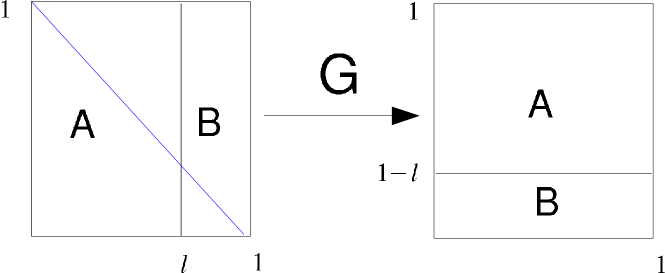
Figure 1: Involution $G$ for the map defined by Eq.(15).

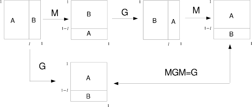
Figure 2: Check of reversibility for the map in Eq.(15), performed by verifying Eq.(2).

The relation $J_{B}=J_{A}^{-1}$ in Eq.(16) is a direct consequence of the time reversibility of the model. To see how this occurs, let us first observe, with the aid of Fig. 2, that the following relations hold for the map Eq.(15):

$$\hskip 85.35826ptGMA=B~{},\quad GMB=A\quad.$$ (18)

Combining this with Eq.(8), we immediately obtain Eq.(16). Relation (8) can be further exploited by introducing the Jacobians of the dynamics restricted to the stable and unstable manifolds in the generic regions $i=\{A,B\}$, which we denote by $J_{i}^{s}$ and $J_{i}^{u}$, respectively. One then has

$$J^{u}_{A}J^{s}_{A}=(J^{u}_{B})^{-1}(J^{s}_{B})^{-1}$$

which, considering the specific constraints of our map, $(J^{u}_{A})^{-1}+(J^{u}_{B})^{-1}=1$ and $J^{s}_{A}+J^{s}_{B}=1$, leads to

$$J^{s}_{A}=(J^{u}_{B})^{-1}\quad\mbox{ and }~{}J^{s}_{B}=(J^{u}_{A})^{-1}\quad.$$ (19)

These equations constitute a consequence, like Eq.(8), of the time-reversibility of the model [11].

A probability density $\rho_{n}$ on $\mathcal{U}$, given at time $n$, evolves according to the Frobenius-Perron equation as [25, 10]

$$\varrho_{n+1}(M(\underline{x}))=J_{M}^{-1}(\underline{x})\>\varrho_{n}(\underline{x})\quad.$$ (20)

Correspondingly, the mean values of a phase function $\mathcal{O}:\mathcal{U}\to I\hskip-3.4ptR$ evolve and can be computed as

$$\langle\mathcal{O}\rangle_{n}=\int_{\mathcal{U}}\mathcal{O}(\underline{x}){\rm d}\mu_{n}(\underline{x})\int_{\mathcal{U}}\mathcal{O}(\underline{x})\rho_{n}(\underline{x})~{}{\rm d}\underline{x}\quad.$$ (21)

If $\langle\mathcal{O}\rangle_{n}$ converges exponentially to a given steady state value $\langle\mathcal{O}\rangle$, for all phase variables $\mathcal{O}$, one says that the state represented by the regular measure $\mu_{n}$ corresponding to the density $\rho_{n}$ converges to a steady state, which yields the asymptotic time statistics of the dynamics. This state will be characterized by an invariant measure $\mu$, which typically is a natural one. For our models this measure is singular, because $M$ is dissipative [39, 25].

However, due to the definition of the map Eq.(15), which stretches distances in the horizontal direction $-$the direction of the unstable manifolds$-$, every application of the map smoothes any initial probability density in that direction, so that our invariant measure is uniform along the $x$-axis. Therefore, to compute steady state averages it is not necessary to use the full information provided by the $n\to\infty$ limit of Eq.(20). Without loss of generality, we may assume that the initial state is “microcanonical”, i.e. its density is uniform in $\mathcal{U}$, $\rho_{0}(x,y)=1$. Then each iteration of the map keeps the density uniform along $x$, while it produces discontinuities in the $y$ direction, so that the $n$-th iterate of the density can be factorized as

$$\rho_{n}(x,y)=C\cdot\hat{\rho}_{n}(y)\quad,$$ (22)

where $\hat{\rho}_{n}$ is a piecewise constant function, which gradually builds up to a fractal structure, and $C$ is a constant that is easily computed to be $1$ by requiring the normalization of $\rho_{n}$. Hence, the varying averages of observables are computed as

$$\langle\mathcal{O}\rangle_{n}\int_{0}^{1}{\rm d}x\int_{0}^{1}{\rm d}y~{}\mathcal{O}(x,y)\hat{\rho}_{n}(y)\quad,$$ (23)

and their steady state values are obtained by taking the limit $n\to\infty$. The average of the phase space contraction rate, which is constant along the $y$-axis, is then easily obtained as

$$\langle\Lambda\rangle_{n} = -\int_{0}^{1}{\rm d}x\int_{0}^{1}{\rm d}y~{}\hat{\rho}_{n}(y)\ln J(x)$$ (24)

$$= \int_{0}^{l}{\rm d}x\ln\frac{r}{l}+\int_{l}^{1}{\rm d}x\ln\frac{l}{r}(l-r)\ln(l/r)\quad.$$

As this result does not depend on $n$, it does not change by taking the limit, and we have $\langle\Lambda\rangle=(l-r)\ln(l/r)$, which vanishes for $l=1/2$ and is positive for all other $l\in(0,1)$. From Eqs.(10) and (16), we can write

$$n~{}\overline{\Lambda}_{n}=(\alpha-\beta)\ln J_{B}\quad,$$ (25)

where $\alpha$ and $\beta=n-\alpha$ denote the number of times the trajectory falls in region $A$ or region $B$, respectively.

To proceed with the derivation of the $\Lambda$-FR for this map, one may now follow two equivalent approaches. First of all, observe that our map is of Anosov type, except for an inessential line of discontinuity, which does not prevent the existence of a Markov partition. Therefore, two basic approaches to the proof of the $\Lambda$-FR may be considered: One may either trust the expansion of the invariant measure in terms of unstable periodic orbits [14, 15], or one may adopt a stochastic approach to the fluctuation relation [25], motivated by the fact that our baker map is isomorphic to a Bernoulli shift, i.e. to a Markov chain whose transition probabilities fulfill

$$p(i_{M^{k}(\underline{x}_{0})};k\rightarrow i_{M^{k+1}(\underline{x}_{0})};k+1)=p(i_{M^{k+1}(\underline{x}_{0})};k+1)\quad,$$

where $i_{M^{k}(\underline{x}_{0})}$, with $k\in[0,n-1]$, denotes the region containing the point $M^{k}(\underline{x}_{0})$, out of the two regions $\{A,B\}$, $p(i_{M^{k}(\underline{x}_{0})};k\rightarrow i_{M^{k+1}(\underline{x}_{0})};k+1)$ denotes the probability that the evolution touches region $i_{M^{k+1}(\underline{x}_{0})}$ at the time step $k+1$, given that it visited the region $i_{M^{k}(\underline{x}_{0})}$ at the previous time step $k$, and $p(i_{M^{k+1}(\underline{x}_{0})};k+1)$ is the probability that $M^{k+1}(\underline{x}_{0})$ belongs to the region $i_{M^{k+1}(\underline{x}_{0})}$. In the $n\rightarrow\infty$ limit, the latter becomes the invariant measure $\mu_{i_{M^{k+1}(\underline{x}_{0})}}$ of the region $i_{M^{k+1}(\underline{x}_{0})}$ itself.

If one uses unstable periodic orbits, the argument proceeds as follows: Every orbit $\omega$ is assigned a weight proportional to the inverse of the Jacobian determinant of the dynamics restricted to its unstable manifold, which is $J_{\omega}^{u}=(J^{u}_{A})^{\alpha}(J^{u}_{B})^{\beta}$, if $\omega$ falls in region $A$ a number $\alpha$ of times and falls in region $B$ a number $\beta$ of times. Then the probability that the dimensionless phase space contraction rate $e_{n}$, computed over a segment of a typical trajectory, falls in the interval $B_{p,\delta}=(p-\delta,p+\delta)$, coincides, in the large $n$ limit, with the sum of the weights of the periodic orbits whose mean phase space contraction rate falls in $B_{p,\delta}$. Denoting this steady state probability by $\pi_{n}(B_{p,\delta})$, one can write

$$\pi_{n}(B_{p,\delta})\approx\frac{1}{N_{n}}~{}\sum_{\omega,e_{n}(\omega)\in B_{p,\delta}}(J_{\omega}^{u})^{-1}\quad,$$ (26)

where $N_{n}$ is a normalization constant, and the approximate equality becomes exact when $n\to\infty$. Because the support of the invariant measure is the whole phase space $\mathcal{U}$, time reversibility guarantees that the support of $\pi_{n}$ is symmetric around $0$, and one can consider the ratio

$$\frac{\pi_{n}(B_{p,\delta})}{\pi_{n}(B_{-p,\delta})}\approx\frac{\sum_{\omega,e_{n}(\omega)\in B_{p,\delta}}(J_{\omega}^{u})^{-1}}{\sum_{\omega,e_{n}(\omega)\in B_{-p,\delta}}(J_{\omega}^{u})^{-1}}~{},$$ (27)

where each $\omega$ in the numerator has a counterpart in the denominator, and the two are related through the involution $G$, as implied by Eq.(12). Therefore, considering each pair of trajectory segments $\omega$ and $\overline{\omega}$, of initial conditions $\underline{x}_{0}$ and $GM^{n}(\underline{x}_{0})$ respectively, Eqs.(12) and (19) imply

$$e_{n}(\omega)=-\overline{e}_{n}(\overline{\omega})~{},\quad(J_{\overline{\omega}}^{u})^{-1}=J_{\omega}^{s}~{},$$ (28)

where, for sake of simplicity, by $e_{n}(\omega)$ we mean the average of $e_{n}(\underline{x}_{0})$, based on any point $\underline{x}_{0}$ of the orbit $\omega$. Consequently, exponentiating the definition of $e_{n}\overline{\Lambda}_{n}/\langle\Lambda\rangle$, and recalling that $J_{\omega}J_{\omega}^{s}J_{\omega}^{u}$, for every orbit $\omega$, we may write

$$\frac{J_{\overline{\omega}}^{u}}{J_{\omega}^{u}}\frac{1}{J_{\omega}^{s}J_{\omega}^{u}}=\frac{1}{J_{\omega}}\exp\left[n\left(\langle\Lambda\rangle p+\epsilon_{\omega}\right)\right]$$ (29)

where $|\epsilon_{\omega}|\leq\delta$ if $e_{n}(\omega)\in B_{p,\delta}$. Because each forward orbit $\omega$ in the denominator of Eq.(27) has a counterpart $\overline{\omega}$ in the denominator, and Eq.(29) holds for each such pair, apart from an error bounded by $\delta$, the whole expression Eq.(27) takes the same value as each of the ratios Eq.(29), with an error $|\epsilon|\leq\delta$,

$$\frac{\pi_{n}(B_{p,\delta})}{\pi_{n}(B_{-p,\delta})}=e^{n\left(\langle\Lambda\rangle p+\epsilon\right)}~{},$$ (30)

where $\epsilon$ can be made arbitrarily small by taking $\delta$ sufficiently small and $n$ sufficiently large. For a given $\delta$, $n$ must also be large because, at every finite $n$, the values which $e_{n}$ takes constitute $2n+1$ isolated points in $[-1,1]$. Therefore, $\pi_{n}(B_{p,\delta})$ vanishes if none of these values falls in $B_{p,\delta}$, making the expression senseless. But the set of these values becomes denser and denser as $n$ increases. Taking the logarithm of Eq.(30), for consistency with Eq.(14), and choosing $p$ among the values $e_{n}$ which may be attained along a periodic orbit of period $n$, we may now write

$$\frac{1}{n\langle\Lambda\rangle}\ln\frac{\pi_{n}(B_{e_{n},\delta})}{\pi_{n}(B_{-e_{n},\delta})}=e_{n}\frac{1}{n\langle\Lambda\rangle}(\alpha-\beta)\ln\left(\frac{l}{r}\right)$$ (31)

for any $\delta>0$. The $n\to\infty$ limit of the above expressions confirms the validity of the $\Lambda$-FR, under the assumption that the unstable periodic orbit expansion could be applied.

From the point of view of the Bernoulli shift description we obtain the same result, supporting the applicability of the the unstable periodic orbit expansion, despite the discontinuity of the dynamics at $l$. Indeed, observe that $l$ equals the probability $\mu_{A}=\int_{A}\mu({\rm d}\underline{x})$ that the trajectory can be found in region $A$, and $r$ equals the probability $\mu_{B}=\int_{B}\mu({\rm d}\underline{x})$ that it is found in region $B$. Therefore, one may write as well

$$\ln\frac{\pi_{n}(B_{e_{n},\delta})}{\pi_{n}(B_{-e_{n},\delta})}\ln\frac{\mu_{A}^{\alpha}\mu_{B}^{\beta}}{\mu_{A}^{\beta}\mu_{B}^{\alpha}}\quad,$$ (32)

which is due to the instantaneous decay of correlations in the Bernoulli process. This leads us to conclude that the violation of the Anosov property, in this simple baker model, is irrelevant for its behavior.

5 The $\Lambda$-FR for a generalized dissipative baker map

We now propose a novel, generalized baker map, which is different from previous models [25, 21, 37, 39, 35] by generating a discontinuity in the invariant density along the $x$-axis. As illustrated in Fig. 3, this is achieved by the map acting differently on four subregions of $\mathcal{U}=[0,1]\times[0,1]$, defined by

$$\left(\begin{array}[]{c}x_{n+1}\\ y_{n+1}\end{array}\right)=M\left(\begin{array}[]{c}x_{n}\\ y_{n}\end{array}\right)=\left\{\begin{array}[]{ll}\left(\begin{array}[]{c}\frac{1}{2l}x_{n}+\frac{1}{2}\\ \\ 2ly_{n}+1-2l\end{array}\right),&\hbox{for $0\leq x<l$;}\\ \left(\begin{array}[]{c}\frac{1}{1-2l}x_{n}-\frac{l}{1-2l}\\ \frac{1}{2}y_{n}+\frac{1}{2}\end{array}\right),&\hbox{for $l\leq x<\frac{1}{2}$;}\\ \left(\begin{array}[]{c}2x_{n}-\frac{1}{2}\\ (1-2l)y_{n}\end{array}\right),&\hbox{for $\frac{1}{2}\leq x<\frac{3}{4}$;}\\ \left(\begin{array}[]{c}2x_{n}-\frac{3}{2}\\ \frac{1}{2}y_{n}\end{array}\right),&\hbox{for $\frac{3}{4}\leq x\leq 1$.}\end{array}\right.\>.$$ (33)

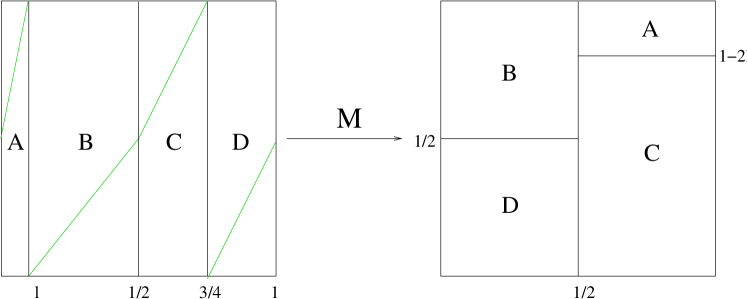
Figure 3: Illustration of the generalized baker map. Green lines: Piecewise linear one-dimensional map, which generates the dynamics along the unstable manifold.

In the sequel, unless stated otherwise, by $M$ we refer to the map introduced in Eq.(33). The model is fixed by choosing the value of $l\in[0,\frac{1}{4}]$, i.e. the width of sub-region $A$. The parameter which determines the dissipation, hence the nonequilibrium steady state, corresponds to a bias $b$ which is suitably defined by $b=J_{C}^{u}-J_{B}^{u}=2-\frac{1}{1-2l}$. According to its geometric construction shown in Fig. 3, the map Eq.(33) is area-contracting in region $B$, area-expanding in region $C$, and area preserving in regions $A$ and $D$. This is confirmed by computing the local Jacobian determinants of the map to

$$J_{M}(\underline{x})=\left\{\begin{array}[]{ll}J_{A}=1,&\hbox{for \quad$0\leq x<l$;}\\ J_{B}=[2(1-2l)]^{-1},&\hbox{for \quad$l\leq x<\frac{1}{2}$;}\\ J_{C}=2(1-2l),&\hbox{for \quad$\frac{1}{2}\leq x<\frac{3}{4}$;}\\ J_{D}=1,&\hbox{for \quad$\frac{3}{4}\leq x\leq 1$.}\end{array}\right.\;.$$ (34)

The following involution $G$,

$$\left(\begin{array}[]{c}x_{G}\\ y_{G}\end{array}\right)=G\left(\begin{array}[]{c}x\\ y\end{array}\right)\left\{\begin{array}[]{ll}\left(\begin{array}[]{c}\frac{1}{2}-\frac{y}{2}\\ 1-2x\end{array}\right),&\hbox{for \quad$0\leq x<\frac{1}{2}$;}\\ \left(\begin{array}[]{c}1-\frac{y}{2}\\ 2-2x\end{array}\right),&\hbox{for \quad$\frac{1}{2}\leq x\leq 1$.}\end{array}\right.\>,$$ (35)

constitutes a time reversal operator for the map $M$ defined on the unit cell. It consists of the composition $G=F\circ S$ of two other involutions, with $S$ permuting the left and the right halfs of the unit square, and $F$ mirroring the regions along their respective diagonals for all values $b\in(-\infty,1]$, cf. Fig. 4.

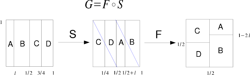
Figure 4: Involution $G$ for the map defined by Eq.(33).

Figure 5: Check of reversibility for the map of Eq.(33), performed by verifying Eq.(2).

Analogously to Eq.(18) for the map Eq.(15), for the generalized map Eq.(33), Eq.(35) entails the relations

$$GMA=A~{},\quad GMD=D~{},\quad GMB=C~{},\quad GMC=B\quad,$$ (36)

which can also be inferred graphically from Fig. 5. It is readily seen, again, that the Jacobian rule Eq.(8), supplemented by Eq.(36), implies the relations Eq.(34).

Let us now lift this biased dissipative baker map onto the whole real line in form of a so-called multibaker map, which consists of an infinitely long chain of baker unit cells deterministically coupled with each other. Multibakers have been studied extensively over the past two decades as simple models of chaotic transport [12, 9, 35, 21, 27, 37]. In our model, which we denote by $M_{mb}$, all unit cells are coupled by shifting the regions $B$ and $C$ to the, respectively, right and left neighboring cells, cf. Fig. 6. Choosing $b\neq 0$, i.e. $l\neq\frac{1}{4}$ then implies the existence of a current $\Psi(b)$, defined by the net flow of points from cell to cell. The map $M_{mb}$ is area contracting (expanding) in the direction (opposite to the direction) of the current, analogously to the case of typical thermostatted particle systems [21, 9]. This can be inferred from the graphical construction in Fig. 6 complemented by the relations Eq.(34).

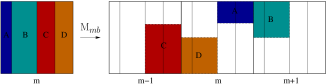
Figure 6: Illustration of a multibaker chain based on the unit cell defined in Fig. 3, featuring a flow of particles from the regions $B$ and $C$ of the cell $m$ into, respectively, the neighboring cell $m+1$ on the right and onto the neighboring cell $m-1$ on the left. The net flow of particles corresponds to the current $\Psi$, which is found to be proportional to the average phase space contraction rate $\langle\Lambda\rangle$.

To asses the validity of the $\Lambda$-FR for this model, let us observe that the form of the invariant probability distribution along the $y$-direction (the direction of the stable manifolds) is irrelevant, analogously to the case discussed in Sec.4, because the phase space contraction per time step, $\Lambda$, does not depend on $y$. By introducing the shorthand notation $\phi=\ln J_{C}$ we have

$$\Lambda(\underline{x})=\Lambda(x,y)\left\{\begin{array}[]{ll}0,&\hbox{for $0\leq x<l$;}\\ \phi,&\hbox{for $l\leq x<\frac{1}{2}$;}\\ -\phi,&\hbox{for $\frac{1}{2}\leq x<\frac{3}{4}$;}\\ 0,&\hbox{for $\frac{3}{4}\leq x\leq 1$.}\end{array}\right.\quad.$$ (37)

The $y$-coordinate may then be integrated out, and one only needs to consider the projection of the invariant measure on the $x$ axis, the direction of the unstable manifolds, which has density $\rho_{x}$.

The calculation of this invariant density can be conveniently performed by introducing a Markov partition of the unit interval, which separates the region $0\leq x<1/2$ from the region $1/2\leq x\leq 1$. Denote by $\rho_{l}$ and $\rho_{r}$ the projected density computed in these two regions and let $T$ be the transfer operator associated with the Markov partition. One may then compute the evolution of the projected densities, which are now piecewise constant, if the initial distribution is uniform on the unit square. In this case the corresponding Frobenius-Perron equation Eq.(20) takes the form [12, 38, 9]

$$\left(\begin{array}[]{c}\rho_{l}(x_{n+1})\\ \rho_{r}(x_{n+1})\end{array}\right)=T\cdot\left(\begin{array}[]{c}\rho_{l}(x_{n})\\ \rho_{r}(x_{n})\end{array}\right)~{},\qquad T=\left(\begin{array}[]{cc}1-2l&1/2\\ 2l&1/2\\ \end{array}\right)\quad.$$ (38)

According to the Perron-Frobenius theorem, the transfer matrix $T$ has largest eigenvalue $\lambda=1$, whose corresponding eigenvector yields the invariant density of the system to

$$\rho(x)\left\{\begin{array}[]{ll}\rho_{l}(x)=\frac{2}{1+4l},&\hbox{for \quad$0\leq x<\frac{1}{2}$;}\\ \rho_{r}(x)=\frac{8l}{1+4l},&\hbox{for \quad$\frac{1}{2}\leq x\leq 1$.}\end{array}\right.\;.$$ (39)

This result confirms that, by construction of the model, and differently from the one considered in Section 4, the density of the map Eq.(33) is not uniform along the $x$-direction, that is, it is actually discontinuous along the unstable direction.

By using this density, the average phase space contraction rate can be calculated to

$$\langle\Lambda\rangle=-\Psi(b)\ln\frac{2-b}{2}\geq 0\quad,$$ (40)

where

$$\Psi(b)=\frac{b}{4-3b}$$ (41)

is the steady state current in the corresponding multibaker chain. Note that

$$\Psi(b)\to\frac{b}{4}\quad(b\to 0)\quad,$$ (42)

hence we have linear response and a caricature of Ohm’s law. Accordingly, we get

$$\langle\Lambda\rangle\to\frac{b^{2}}{8}\quad(b\to 0)$$ (43)

for the average phase space contraction rate, as one would expect from nonequilibrium thermodynamics if this quantity was identified with the nonequilibrium entropy production rate of a system [21, 35]. This confirms that our abstract map represents a ‘reasonably good toy model’ in capturing some properties as they are expected to hold for ordinary nonequilibrium processes. Related biased one-dimensional maps have been studied in Refs. [40, 9]. Note that $\Psi=0$ for $l=1/4$, respectively $b=0$, only, in which case the dynamics is conservative, and the model boils down to a special case of the multibaker map analyzed in Ref. [38].

In order to check the $\Lambda$-FR for this model, we first need to define the transition probabilities $p_{ij}$ of jumping from region $i$ to region $j$, with $i,j\in\{A,B,C,D\}$ denoting the finite state space. They constitute the elements of the transition matrix

$$P=\left(\begin{array}[]{cccc}0&0&\frac{1}{2}&\frac{1}{2}\\ 2l&1-2l&0&0\\ 0&0&\frac{1}{2}&\frac{1}{2}\\ 2l&1-2l&0&0\\ \end{array}\right)\quad.$$ (44)

Note that $P$ defines a stochastic transition matrix, which acts onto vectors whose elements are the probabilities to be in the different regions, in contrast to the topological transition matrix Eq.(38), which acts upon probability density vectors. The left eigenvector of $P$, associated with the eigenvalue $1$, corresponds to the vector of the invariant probabilities $\mu_{i}$ of the regions $A,B,C$ and $D$. Alternatively, since the projected invariant probability density is constant in each of these four regions, the $\mu_{i}$’s are also immediately obtained by multiplying the relevant invariant density Eq.(39) with the width of the respective region. One way or the other, we obtain

$$\mu_{i}\left\{\begin{array}[]{ll}\frac{2l}{1+4l},&\hbox{if ~{} $i=A,C,D$;}\\ \frac{1-2l}{1+4l},&\hbox{if ~{} $i=B$.}\end{array}\right.\quad.$$ (45)

The discontinuity of the invariant density Eq.(39) along the unstable direction, for $l\neq 1/4$, means that the Anosov property is more substantially violated here than for the map in Section 4. Therefore, the periodic orbit expansion used in Section 4 cannot be immediately trusted, and an alternative method is better suited to prove the validity of the $\Lambda$-FR.

We may begin by considering a trajectory segment of $n$ steps, which starts at $\underline{x}_{0}\in i_{\underline{x}_{0}}$ and ends in $\underline{x}_{n}\in i_{\underline{x}_{n}}$, hence visits the regions $\{i_{\underline{x}_{0}},...,i_{\underline{x}_{n}}\}$. Consider the first $(n-1)$ transitions, corresponding to the symbol sequence $\{i_{\underline{x}_{0}},...,i_{\underline{x}_{n-1}}\}$, and treat separately the last transition $i_{\underline{x}_{n-1}}\rightarrow i_{\underline{x}_{n}}$. Denote by $n_{ij}$ the number of transitions from region $i$ to region $j$, along the trajectory segment of $(n-1)$ steps, and by $n_{i}=\sum_{\{j:p_{ij}\neq 0\}}n_{ij}$ the total number of transitions starting in $i$. Some transitions are forbidden, as shown by Eq.(44), hence the following holds:

$$\underbrace{n_{AC}+n_{AD}}_{n_{A}}+\underbrace{n_{BA}+n_{BB}}_{n_{B}}+\underbrace{n_{CC}+n_{CD}}_{n_{C}}+\underbrace{n_{DA}+n_{DB}}_{n_{D}}=n-1\quad.$$

It also proves convenient to introduce the following symbols:

$$n_{\rightsquigarrow i}\left\{\begin{array}[]{ll}0,&\hbox{if the trajectory does not start in $i$;}\\ 1,&\hbox{if the trajectory starts in $i$.}\end{array}\right.$$ (46)

$$n_{i\rightsquigarrow}\left\{\begin{array}[]{ll}0,&\hbox{if the trajectory does not end in $i$;}\\ 1,&\hbox{if the trajectory ends in $i$.}\end{array}\right.$$ (47)

and $\Delta_{ij}=n_{\rightsquigarrow i}-n_{j\rightsquigarrow}$. The quantities $n_{\rightsquigarrow i}$ and $n_{i\rightsquigarrow}$ take into account the possibility that the trajectory segment may, respectively, start in, or end into, the region $i$. Thus, we may write the following flux balances

$$\sum_{\{i:p_{ij}\neq 0\}}n_{ij}=n_{j}-\Delta_{jj},\quad\forall j$$ (48)

for each region of the map. Next, we introduce the quantity

$$g=n_{B}-n_{C}+n_{B\rightsquigarrow}-n_{C\rightsquigarrow}\quad,$$ (49)

which lies in the interval $[-n,n]$ and is related by

$$\overline{\Lambda}_{n}={g}\phi/n$$ (50)

to the average phase space contraction in a trajectory segment of $n$ steps.

To evaluate the ratio of probabilities appearing in the $\Lambda$-FR, let us denote by $i_{\underline{x}}$ the region containing the point $\underline{x}$, out of the four regions $\{A,B,C,D\}$, and let us focus on a single trajectory of initial condition $\underline{x}_{0}=(x_{0},y_{0})\in i_{\underline{x}_{0}}$. For a given $n$, the sequence of transitions which take this point from region $i_{\underline{x}_{0}}$ to region $i_{M(\underline{x}_{0})}=i_{\underline{x}_{1}}$, from region $i_{\underline{x}_{1}}$ to region $i_{M^{2}(\underline{x}_{0})}=i_{\underline{x}_{2}}$ and eventually from region $i_{M^{n-1}(\underline{x}_{0})}=i_{\underline{x}_{n-1}}$ to region $i_{M^{n}(\underline{x}_{0})}=i_{\underline{x}_{n}}$ does not depend on $y_{0}$. The larger the value of $n$, the narrower the width of the set of initial conditions whose trajectories undergo the same sequence of $n$ transitions experienced by the trajectory starting in $\underline{x}_{0}$. Let $\omega(\underline{x}_{0},n)=\{\underline{x}\in\mathcal{U}:M^{k}(\underline{x})\in i_{M^{k}(\underline{x}_{0})},k=0,...,n\}\subset i_{\underline{x}_{0}}$ denote this set of initial conditions. The expansiveness of the map implies

$$\lim_{n\to\infty}\omega(\underline{x}_{0},n)=\left\{\underline{x}=(x,y):x=x_{0},y\in[0,1]\right\}~{}.$$

Because the phase space contraction $\Lambda(\underline{x}_{k})$ only depends on the region $i_{\underline{x}_{k}}$ from which the transition $i_{\underline{x}_{k}}\to i_{\underline{x}_{k+1}}$ occurs, all trajectory segments of $n$ steps originating in $\omega(\underline{x}_{0},n)$ enjoy the same average phase space contraction $\overline{\Lambda}_{n}$. The amount $\overline{\Lambda}_{n}$ is also produced by the trajectory segments which visit the regions $i_{\underline{x}_{0}},...,i_{\underline{x}_{n-1}}$ and eventually land in $i_{\underline{\hat{x}}_{n}}$, where $i_{\underline{\hat{x}}_{n}}\neq i_{\underline{x}_{n}}$ is the other region reachable from $i_{\underline{x}_{n-1}}$. Let $\omega(\underline{\hat{x}}_{0},n)$ be this second set of initial conditions producing $\overline{\Lambda}_{n}$ in $n$ steps. The point $\underline{\hat{x}}_{0}$ lies in $i_{\underline{x}_{0}}$, i.e. $i_{\underline{\hat{x}}_{0}}=i_{\underline{x}_{0}}$, but differs from ${\underline{x}_{0}}$ and does not belong to $\omega(\underline{x}_{0},n)$. Denoting by $\pi_{\omega(\underline{x}_{0},n)}$ the invariant measure of $\omega(\underline{x}_{0},n)$, one finds:

$$\pi_{\omega(\underline{x}_{0},n)}$$

$$=\mu_{i_{\underline{x}_{0}}}\prod_{k=0}^{n-2}p(i_{M^{k}\underline{x}_{0}};k\rightarrow i_{M^{k+1}\underline{x}_{0}};k+1)p(i_{M^{n-1}(\underline{x}_{0})},n-1\rightarrow i_{M^{n}(\underline{x}_{0})};n)$$

$$=\mu_{i_{\underline{x}_{0}}}p_{AC}^{n_{AC}}p_{AD}^{n_{AD}}p_{BA}^{n_{BA}}p_{BB}^{n_{BB}}p_{CC}^{n_{CC}}p_{CD}^{n_{CD}}p_{DA}^{n_{DA}}p_{DB}^{n_{DB}}p(i_{M^{n-1}(\underline{x}_{0})};n-1\rightarrow i_{M^{n}(\underline{x}_{0})};n)$$

$$=\mu_{i_{\underline{x}_{0}}}p_{DA}^{n_{BA}+n_{DA}}p_{BB}^{n_{BB}+n_{DB}}p_{CC}^{n_{AC}+n_{CC}}p_{AD}^{n_{AD}+n_{CD}}p(i_{M^{n-1}(\underline{x}_{0})};n-1\rightarrow i_{M^{n}(\underline{x}_{0})};n)$$

$$=\mu_{i_{\underline{x}_{0}}}p_{DA}^{n_{A}-\Delta_{AA}}p_{BB}^{n_{B}-\Delta_{BB}}p_{CC}^{n_{C}-\Delta_{CC}}p_{AD}^{n_{D}-\Delta_{DD}}\times$$

$$\times p(i_{M^{n-1}(\underline{x}_{0})};n-1\rightarrow i_{M^{n}(\underline{x}_{0})};n)\>,$$ (51)

where we made use of Eqs.(48) and of the equalities $p_{ij}=p_{kj}$ for all $i\neq j$, which can be deduced from an inspection of Eq.(44). Similarly, one has

$$\pi_{\omega(\underline{\hat{x}}_{0},n)}=\mu_{i_{\underline{x}_{0}}}p_{DA}^{n_{A}-\Delta_{AA}}p_{BB}^{n_{B}-\Delta_{BB}}p_{CC}^{n_{C}-\Delta_{CC}}p_{AD}^{n_{D}-\Delta_{DD}}p(i_{M^{n-1}(\underline{x}_{0})};n-1\rightarrow i_{\underline{\hat{x}}_{n}};n)~{}.$$ (52)

Given the similarity of the expressions Eqs.(51) and (52), and the fact that

$$p(i_{M^{n-1}(\underline{x}_{0})},n-1\rightarrow i_{M^{n}(\underline{x}_{0})};n)+p(i_{M^{n-1}(\underline{x}_{0})};n-1\rightarrow i_{\underline{\hat{x}}_{n}};n)=1~{},$$ (53)

it is convenient to consider the set

$$\omega(\underline{x}_{0},n)\cup\omega(\underline{\hat{x}}_{0},n)=\omega(\underline{x}_{0},n-1)$$ (54)

whose measure is given by

$$\pi_{\omega(\underline{x}_{0},n-1)}=\mu_{i_{\underline{x}_{0}}}p_{DA}^{n_{A}-\Delta_{AA}}p_{BB}^{n_{B}-\Delta_{BB}}p_{CC}^{n_{C}-\Delta_{CC}}p_{AD}^{n_{D}-\Delta_{DD}}\quad.$$ (55)

This measure represents the contribution to the probability of producing $\overline{\Lambda}_{n}$ in $n$ steps, given by the trajectory segments whose initial conditions lie in $\omega(\underline{x}_{0},n-1)$. The steady state probability of $\overline{\Lambda}_{n}$ is then the sum of contributions like Eq.(55), for all remaining sets of trajectories compatible with $\overline{\Lambda}_{n}$, characterized by distinct sequences of $n-1$ transitions.

As we discussed at the end of Section 2, for any initial point $\underline{x}_{0}$ in the phase space that experiences a mean phase space contraction $\overline{\Lambda}_{n}(\underline{x}_{0})$ in $n$ steps, the point $\underline{x}_{0R}=GMM^{n-1}(\underline{x}_{0})=GM^{n}(\underline{x}_{0})$ experiences the opposite mean phase space contraction $\overline{\Lambda}_{n}(\underline{x}_{0R})=-\overline{\Lambda}_{n}(\underline{x}_{0})$, cf. Eq.(12). The trajectory segment of $n$ steps, starting at $\underline{x}_{0R}$, is thus the time reversal of the one starting at $\underline{x}_{0}$, and ${\omega}(GM^{n}(\underline{x}_{0}),n)$ is the set of initial conditions of the time reversals of the segments beginning in $\omega(\underline{x}_{0},n)$. The segments beginning in ${\omega}(GM^{n}(\underline{x}_{0}),n)$ visit the regions $i_{GM^{n}(\underline{x}_{0})}$, $i_{GM^{n-1}(\underline{x}_{0})}$, … $i_{G(\underline{x}_{0})}$, hence they produce the average phase space contraction $-\overline{\Lambda}_{n}$ if the segments beginning in $\omega(\underline{x}_{0},n)$ produce $\overline{\Lambda}_{n}$. In analogy to Eq.(51) their steady state probability is given by:

$$\pi_{{\omega}(GM^{n}(\underline{x}_{0}),n)} = \mu_{i_{GM^{n}(\underline{x}_{0})}}\prod_{k=0}^{n-2}p(i_{GM^{n-k}(\underline{x}_{0})};k\rightarrow i_{GM^{n-k-1}(\underline{x}_{0})};k+1)\times$$ (56)

$$\times p(i_{GM(\underline{x}_{0})};n-1\rightarrow i_{G(\underline{x}_{0})};n)\>.$$

Figure 7: Sequence of visited regions in the forward (upper sequence) and time-reversed (lower sequence) dynamics. The lower sequence is determined by applying the composite map $G\circ M$ onto the upper sequence, cf. Eq. (36) (thick blue arrows).

Again, this set of trajectories may be grouped together with the set of trajectories whose last step falls in the other region reachable from $Gi_{\underline{x}_{1}}$, say $\hat{i}_{\underline{x}_{0}}\neq i_{\underline{x}_{0}}$. The probability of the union ${\omega}(GM^{n}(\underline{x}_{0}),n-1)$ of these two sets takes the value

$$\pi_{\omega(GM^{n}(\underline{x}_{0}),n-1)} = \mu_{i_{GM^{n}(\underline{x}_{0})}}\prod_{k=0}^{n-2}p(i_{GM^{n-k}(\underline{x}_{0})};k\rightarrow i_{GM^{n-k-1}(\underline{x}_{0})};k+1)$$ (57)

$$= \mu_{GMi_{M^{n-1}(\underline{x}_{0})}}p_{BA}^{n_{AC}}p_{DA}^{n_{AD}}p_{AC}^{n_{BA}}p_{CC}^{n_{BB}}p_{BB}^{n_{CC}}p_{DB}^{n_{CD}}p_{AD}^{n_{DA}}p_{CD}^{n_{DB}}$$

$$= \mu_{GMi_{M^{n-1}(\underline{x}_{0})}}p_{DA}^{n_{A}}p_{CC}^{n_{B}}p_{BB}^{n_{C}}p_{AD}^{n_{D}}\quad,$$

where we have made use, from Eq.(36), of the crucial relation $i_{GM^{k}(\underline{x}_{0})}=GMi_{M^{k-1}(\underline{x}_{0})}$, with $k=1,...,n$, cf. Fig. 7. This contribution to the probability of producing $-\overline{\Lambda}_{n}$ in $n$ steps mirrors the contribution to the probability of producing $\overline{\Lambda}_{n}$, given by Eq.(55). Taking the ratio of these two contributions and writing the phase space contraction in terms of $g$ units of size $\phi$, cf. Eq.(50), one obtains

$$\frac{\pi_{\omega(\underline{x}_{0},n-1)}}{\pi_{\omega(GM^{n}(\underline{x}_{0}),n-1)}} = \frac{\mu_{i_{\underline{x}_{0}}}}{\mu_{GMi_{M^{n-1}(\underline{x}_{0})}}}\frac{p_{DA}^{n_{A}-\Delta_{AA}}p_{BB}^{n_{B}-\Delta_{BB}}p_{CC}^{n_{C}-\Delta_{CC}}p_{AD}^{n_{D}-\Delta_{DD}}}{p_{DA}^{n_{A}}p_{CC}^{n_{B}}p_{BB}^{n_{C}}p_{AD}^{n_{D}}}$$ (58)

$$= \left(\frac{p_{BB}}{p_{CC}}\right)^{g}\alpha_{\omega}$$

with

$$\alpha_{min}\leq\alpha_{\omega}=\left[\frac{\mu_{i_{\underline{x}_{0}}}}{\mu_{GMi_{M^{n-1}(\underline{x}_{0})}}}p_{DA}^{-\Delta_{AA}}p_{BB}^{-\Delta_{BC}}p_{CC}^{-\Delta_{CB}}p_{AD}^{-\Delta_{DD}}\right]\leq\alpha_{max}\quad,$$ (59)

where the upper and lower bounds $\alpha_{min}$ and $\alpha_{max}$ are $(g,n)$-independent positive numbers, which are found to be

$$\alpha_{min}=4l=\alpha_{max}^{-1}\quad,$$ (60)

as we numerically tested by considering all possible values of $\alpha_{\omega}$ corresponding to a trajectory segment visiting the regions $i_{\underline{x}_{0}},...,i_{M^{n-1}(\underline{x}_{0})},i_{M^{n}(\underline{x}_{0})}$, for any $i_{\underline{x}_{0}},i_{M^{n-1}(\underline{x}_{0})}$ and $i_{M^{n}(\underline{x}_{0})}$. At the same time, Eqs.(44) and (45) imply the equality being at the heart of the $\Lambda$-FR, i.e.

$$\left(\frac{p_{BB}}{p_{CC}}\right)^{g}=e^{g\phi}\quad.$$

These results hold for all sets of trajectory segments starting in ${\omega}(\underline{x}_{0},n-1)$, related to their corresponding reversals starting in ${\omega}(GM^{n}(\underline{x}_{0}),n-1)$. Therefore, Eq.(58) holds as well for the total probabilities of producing $\overline{\Lambda}_{n}$ and $-\overline{\Lambda}_{n}$, because the ratio of the sums of the probabilities of the groups of trajectory segments producing $\overline{\Lambda}_{n}$ and $-\overline{\Lambda}_{n}$ equals the ratio of the probabilities of a single group, with corrections always bounded by $\alpha_{min}$ and $\alpha_{max}$.

To match this result with the $\Lambda$-FR Eq.(14), it now suffices to introduce the normalized quantity $e_{n}=g\phi/n\langle\Lambda\rangle$ and to take the logarithm of the ratio of probabilities,

$$e_{n}(\underline{x})-{\frac{\ln\alpha_{max}}{n\langle\Lambda\rangle}}\leq\frac{1}{n\langle\Lambda\rangle}\ln\frac{\mu(\{\underline{x}:e_{n}(\underline{x})\in(p-\delta,p+\delta)\})}{\mu(\{\underline{x}:e_{n}(\underline{x})\in(-p-\delta,-p+\delta)\}}\leq e_{n}(\underline{x})+{\frac{\ln\alpha_{max}}{n\langle\Lambda\rangle}}\>.$$ (61)

In the ${n\rightarrow\infty}$ limit, in which the allowed values of $e_{n}$ become dense in the domain of the $\Lambda$-FR, one recovers the fluctuation theorem with $p^{*}=\phi/\langle\Lambda\rangle$.

6 Conclusions

In this paper we have presented analytically tractable examples of dynamical systems in order to clarify some aspects of the applicability of the standard steady state fluctuation relation. In our case, there is no distinction between the so-called $\Lambda$-FR and $\Omega$-FR, because the appropriate measure is the Lebesgue measure, in our case, cf. Eq.(9) [4, 16]. Our results show that the $\Lambda$-FR holds under less stringent conditions than those required by the Gallavotti-Cohen FT, which include time reversibility and existence of an SRB measure, i.e. a measure which is smooth along the unstable directions. This is of interest for applications, because strong requirements such as the Anosov property are hardly met by dynamics of physical interest, in general.

To obtain this result, we have considered an example in which the involution representing the time reversal operator is discontinuous [17] and in which also the invariant measure is discontinuous along the unstable direction. Our discontinuities are mild, as discussed in the introduction, however, they illustrate how the validity of the $\Lambda$-FR may be extended beyond the standard constraints. Our proof capitalizes on the fact that the directions of stable and unstable manifolds are fixed and that the vertical variable does not affect the value of the phase space contraction rate. This fact has rather profound implications concerning the validity of the $\Lambda$-FR for cases in which time reversibility is more substantially violated. In fact, only the knowledge of the forward and reversed sequences of visited regions is required in order to verify the $\Lambda$-FR, rather than the more detailed knowledge of the forward and reversed trajectories in phase space. Thus, for instance, one easily realizes that our calculations may be carried out for a map of the form $K=M\circ N$, where $M$ may refer to one of the maps Eqs.(15) or (33), while $N$ does not contract or expand volumes and affects in some irreversible fashion the $y$-coordinate only. $N$ can be constructed in several ways: For example, let $M$ be the map Eq.(33), and assume that $N$ acts only on a vertical strip of width $\epsilon$ in the region $B$, as follows:

$$\left(\begin{array}[]{c}x_{n+1}\\ y_{n+1}\end{array}\right)=N\left(\begin{array}[]{c}x_{n}\\ y_{n}\end{array}\right)\left\{\begin{array}[]{ll}\left(\begin{array}[]{c}x_{n}\\ 1-y_{n}\end{array}\right),&\hbox{for $x\in[\tilde{x},\tilde{x}+\epsilon]$ and $y\in[0,\frac{1}{2}]$;}\\ \left(\begin{array}[]{c}x_{n}\\ y_{n}\end{array}\right)&\hbox{for $x\in[\tilde{x},\tilde{x}+\epsilon]$ and $y\in(\frac{1}{2},1]$.}\end{array}\right.\>.$$ (62)

cf. Fig.8 for a graphical representation. The map $N$ is not reversible, according to the definition Eq.(2); in fact, $N$ is not even a homeomorphism, as its inverse $N^{-1}$ is not defined, so neither is the inverse of the composite map $K^{-1}$. Nevertheless, the $\Lambda$-FR still holds in this case, due to the existence of a milder notion of reversibility expressed by the relations Eq.(36). The latter entail that only a coarse-grained involution, mapping regions onto regions, is needed for the proof of the $\Lambda$-FR, rather than a local involution, mapping points into points in phase space, as defined by Eq.(2).

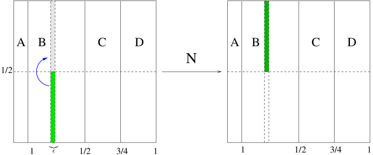
Figure 8: The map $N$ defined in Eq.(62), which spoils the reversibility of the model

7 Acknowledgements

M.C. acknowledges support from the Swiss National Science Foundation (SNSF). R.K. is grateful to Ramses van Zon for helpful discussions on time-reversibility. L.R. and P.D.G. gratefully acknowledge financial support from the European Research Council under the European Community’s Seventh Framework Programme (FP7/2007-2013) / ERC grant agreement n 202680. The EC is not liable for any use that can be made on the information contained herein.

References

References

- [1] U. Marini Bettolo Marconi, A. Puglisi, L. Rondoni, A. Vulpiani: Fluctuation-Dissipation: Response Theory in Statistical Physics, Phys. Rep. 461, 111 (2008).
- [2] R. Chetrite, K. Gawedzki: Fluctuation relations for diffusion processes, Comm. Math. Phys. 282, 2, 469 (2008).
- [3] V. Jaksic, C.-A. Pillet, L. Rey-Bellet: Entropic Fluctuations in Statistical Mechanics I. Classical Dynamical Systems, Nonlinearity 24, 699 (2011).
- [4] D. J. Searles, L. Rondoni, D. J. Evans: The steady state fluctuation relation for the dissipation function, J. Stat. Phys. 128, 1337 (2007).
- [5] O. G. Jepps, L. Rondoni: Deterministic thermostats, theories of nonequilibrium systems and parallels with the ergodic condition, J. Phys. A: Mathematical and Theoretical 43, 1 (2010).
- [6] G. Gonnella, A. Pelizzola, L. Rondoni, G. P. Saracco: Nonequilibrium work fluctuations in a driven Ising model, Physica A 388, 2815 (2009).
- [7] M. Bonaldi, L. Conti, P. De Gregorio, L. Rondoni, G. Vedovato, A. Vinante, M. Bignotto, M. Cerdonio, P. Falferi, N. Liguori, S. Longo, R. Mezzena, A. Ortolan, G.A. Prodi, F. Salemi, L. Taffarello, S. Vitale, J.P. Zendri: Nonequilibrium Steady-State Fluctuations in Actively Cooled Resonators, Phys. Rev. Lett. 103, 010601 (2009).
- [8] D. J. Evans, G. P. Morriss: Statistical Mechanics of Nonequilibrium Liquids (Academic Press, London, 1990); W. G. Hoover: Computational Statistical Mechanics (Elsevier, Amsterdam, 1991).
- [9] R. Klages: Microscopic chaos, fractals and transport in nonequilibrium statistical mechanics (Singapore, World Scientific, 2007).
- [10] A. Lasota, M.C.Mackey: Chaos, Fractals, and Noise. Stochastic Aspects of Dynamics (Cambridge University Press, 1985).
- [11] D. Ruelle: Smooth dynamics, new theoretical ideas in nonequilibrium statistical mechanics, J. Stat. Phys. 95, 393 (1999).
- [12] P. Gaspard: Chaos, Scattering, and Statistical Mechanics (Cambridge University Press, Cambridge, 1998).
-
[13]
D. J. Evans, E. G. D. Cohen, M. P. Morris:
Viscosity of a simple fluid from its maximal Lyapunov exponent,
Phys. Rev. A 42, 5990 (1990);
N. I. Chernov, G. L. Eyink, J. L. Lebowitz, Ya. G. Sinai: Derivation of Ohm’s law in a deterministic mechanical model, Phys. Rev. Lett. 70, 2209 (1993). - [14] G. P. Morris, L. Rondoni: Periodic Orbit Expansions for the Lorentz Gas, J. Stat. Phys.75, 553 (1994).
- [15] P. Cvitanovic, R. Artuso, R. Mainieri, G. Tanner, G. Vattay, N. Whelan, A. Wirzba: Chaos: Classical and quantum, http://chaosbook.org/.
- [16] L. Rondoni, C. Mejia-Monasterio: Fluctuations in nonequilibrium statistical mechanics:models, mathematical theory, physical mechanisms, Nonlinearity 20, p. R1-R37 (2007).
- [17] M. Porta: Fluctuation theorem, nonlinear response, and the regularity of time reversal symmetry, Chaos 20, 023111 (2010).
- [18] D.J. Evans, E. G. D. Cohen, G. P. Morriss: Probability of second law violations in nonequilibrium steady states, Phys. Rev. Lett. 71, 2401 (1993).
-
[19]
G. Gallavotti, E. G. D. Cohen:
Dynamical Ensembles in Nonequilibrium Statistical Mechanics,
Phys. Rev. Lett. 74, 2694 (1995);
G. Gallavotti, E. G. D. Cohen: Dynamical Ensembles in stationary states, J. Stat. Phys. 80, 931 (1995). - [20] G. Gallavotti: Chaotic dynamics, fluctuations, nonequilibrium ensembles, Chaos 8 (2), 384 (1998).
-
[21]
T. Tél, J. Vollmer, W. Breymann:
Transient chaos: the origin of transport in driven systems,
Europhys. Lett. 35, 659 (1996);
J. Vollmer, T. Tél, W. Breymann: Equivalence of Irreversible Entropy Production in Driven Systems: An Elementary Chaotic Map Approach, Phys. Rev. Lett. 79, 2759 (1997). - [22] J. A. G. Roberts, G. R. W. Quispel: Chaos and time-reversal symmetry. Order and chaos in reversible dynamical systems, Phys. Rep. 216, 63 (1992).
- [23] S. Ciliberto, S. Joubaud, A. Petrosyan: Fluctuations in out of equilibrium systems: from theory to experiment, J. Stat. Mech. (2010) P12003.
- [24] D. J. Evans, D. J. Searles: The fluctuation theorem, Adv. Phys. 52, 1529 (2002).
- [25] J. R. Dorfman: An introduction to Chaos in Nonequilibrium Statistical Mechanics (Cambridge Lecture Notes in Physics, 2001).
- [26] D. J. Evans, S. J. Searles, L. Rondoni: On the application of the Gallavotti-Cohen fluctuation relation to thermostatted steady states near equilibrium, Phys. Rev. E 71, 056120 (2005).
-
[27]
L. Rondoni, E.G.D. Cohen:
Gibbs entropy and irreversible thermodynamics,
Nonlinearity, 13, 1905 (2000);
L. Rondoni, E. G. D. Cohen: On some derivations of irreversible thermodynamics form dynamical systems theory, Physica D: Nonlinear Phenomena 168-169, 341 (2002). - [28] D. J. Evans, D. J. Searles: Equilibrium microstates which generate second law violating steady states, Phys. Rev. E 50, 1645 (1994).
- [29] L. Rondoni, G. P. Morriss: Large fluctuations and axiom-C structures in deterministically thermostatted systems, Open Syst.& Inform. Dyn. 10, 105 (2003).
- [30] C. Mejia-Monasterio, L. Rondoni: On the Fluctuation Relation for Nos -Hoover Boundary Thermostated Systems, J. Stat. Phys. 133, 617 (2008).
- [31] F. Bonetto, G. Gallavotti: Reversibility, coarse graining and the chaoticity principle, Commun. Math. Phys. 189, 263 (1997).
- [32] L. Rondoni: Deterministic thermostats and fluctuation relations, in: Dynamics of Dissipation, Lecture Notes in Physics 597 ed. P Garbaczewski and R Olkiewicz (Springer, Berlin, 2002).
- [33] G. Benettin, L. Rondoni: A new model for the transport of particles in a thermostatted system, Math. Phys. Electron. J. 7, 3 (2001).
- [34] A. V. Chechkin, R. Klages: Fluctuation relations for anomalous dynamics, J.Stat.Mech. (2009) L03002.
- [35] J. Vollmer: Chaos, spatial extension, transport, and non-equilibrium thermodynamics, Phys. Rep. 372, 131 (2002).
- [36] L. Rondoni, T. Tel, J. Vollmer: Fluctuation theorems for entropy production in open systems, Phys. Rev. E 61, R4679-R4682 (2000).
- [37] T. Gilbert, J. R. Dorfman: Entropy production: From open volume-preserving to dissipative systems, J. Stat. Phys. 96, 225 (1999)
- [38] P. Gaspard, R. Klages: Chaotic and fractal properties of deterministic diffusion-reaction processes, Chaos 8, 409 (1998).
- [39] S. Tasaki, T. Gilbert, J. R. Dorfman: An analytical construction of the SRB measures for Baker-type maps, Chaos 8, 424 (1998).
- [40] J. Groeneveld, R. Klages: Negative and nonlinear response in an exactly solved dynamical model of particle transport, J. Stat. Phys. 109, 821 (2002).
- [41] J. S.W. Lamb: Area-preserving dynamics that is not reversible, Physica A 228, 1, 344 (1996)
- [42] J. L. Lebowitz, H. Spohn: A Gallavotti-Cohen-Type Symmetry in the Large Deviation Functional for Stochastic Dynamics, J. Stat. Phys. 95, 333 (1999).