Stiffness in 1D Matrix Product States with periodic boundary conditions

Abstract

We discuss in details a modified variational matrix-product-state algorithm for periodic boundary conditions, based on a recent work by P. Pippan, S.R. White and H.G. Everts, Phys. Rev. B 81 (2010) 081103(R), which enables one to study large systems on a ring (composed of $N\sim 10^{2}$ sites). In particular, we introduce a couple of improvements that allow to enhance the algorithm in terms of stability and reliability. We employ such method to compute the stiffness of one-dimensional strongly correlated quantum lattice systems. The accuracy of our calculations is tested in the exactly solvable spin-1/2 Heisenberg chain.

1 Introduction

The recent technological advances in manipulating cold atomic gases with very high control and accuracy have opened up the possibility to test the quantum physics of many-particle systems in its roots [1]. Moreover, quantum many-body systems can sustain collective states of matter which have no classical analog, such as superfluid or insulating quantum phases [2], or even more exotic states such as the supersolid [3]. Experimental achievements along these direction renewed, in parallel, a considerable theoretical interest in the study of strongly correlated systems. Unfortunately, despite the apparent simplicity of their constituting Hamiltonian, the lack of a dominant exactly solvable contribution ultimately limits the applicability of conventional perturbative methods, thus drastically restricting analytic studies of both statics and non-equilibrium dynamical properties to very few cases. Approximated techniques or fully numerical approaches are therefore often required.

In the early Nineties, White proposed a very powerful and accurate algorithm for numerically performing the renormalization group procedure in one-dimensional (1D) systems [4]. Its large applicability to the study of both static and dynamic properties of the low-energy spectrum of generic strongly correlated 1D quantum systems, stimulated a considerable part of condensed matter theorists, which, in the subsequent years, produced a number of relevant results lying on this method, also called the Density Matrix Renormalization Group (DMRG) (see, e.g., Ref. [5] and references therein). The formal equivalence of the DMRG procedure with a Matrix Product State (MPS) [6], which can be written in terms of a product of certain matrices, permitted a reformulation of the DMRG method as an optimization algorithm. This allowed a better understanding of the renormalization procedure, together with a number of promising extensions and improvements of the method, mostly coming from quantum information communities. Nonetheless, unlike the original DMRG protocol, these new algorithms are still not of common use and their potentialities have not been completely exploited [7].

One of the drawbacks of the celebrated DMRG algorithm, in its canonical formulation, is its intrinsic difficulty in simulating ground states of 1D systems with periodic boundary conditions. In particular, the accuracy scales like the square of the number of states kept in an analogous simulation with open boundary conditions [4]. For this reason, its applicability to systems closed on a ring is limited to very few examples in the literature [8]. Much better performances can be obtained by reformulating the DMRG in terms of a variational procedure on the class of MPS with periodic boundaries [9]. This is done at the expense of no longer using sparse matrices, thus reflecting in a considerable slowdown of the procedure; moreover, due to the cyclic structure of the MPS, contractions of the various matrices also become more costly. However, from a conceptual point of view, the accuracy should drastically increase, since the original DMRG was equivalent to an optimization method in which the variational class of states intrinsically belonged to the MPS with open boundaries. Clever strategies for reducing the computational cost of such algorithms, in the case of translational invariant MPS, have been developed in Refs. [10, 11, 12] and tested using Heisenberg and Ising spin-1/2 chains as benchmark models. Very recently, an improved version of the algorithm in Ref. [9], for generic non-translationally invariant systems, has been put forward by Pippan et al. [13]. As we will outline in the following, this enables a great computational speedup, so that precisions of the same order of magnitude of the ones obtained with open boundaries can be reached with a reasonable computational cost.

The purpose of this paper is twofold. First we present in detail an optimized variational MPS algorithm for periodic boundary conditions, which enables one to study static properties of the ground state of large, generically non-homogeneous, systems on a ring (made up of $N\sim 10^{2}$ sites). The most important steps of the algorithm are those of Ref. [13], we present however a number of suggestions that improve its stability. Specifically, first we provide a way to stabilize the generalized eigenvalue problem that has to be solved at each variational step. This consists in   i) suitably choosing the gauge conditions for the MPS, as previously hinted in Ref. [14], and then in   ii) wiping out the kernel of the effective norm operator by introducing small perturbative corrections in the effective operators. Furthermore, we also employ the decomposition of products of Ref. [13], other than for multiplying transfer matrices, also to simplify the decomposition of the effective Hamiltonian, thus speeding up its diagonalization. The capabilities of the algorithm and the scaling of the precision with the dimension of the MPS are the same as those in the standard DMRG algorithm. Putting emphasis on all the major technical details of our algorithm, we aim at providing a rather comprehensive explanation which reveals itself compulsory for everybody who wants to implement it operatively.

The second purpose of the paper is to employ the algorithm in order to numerically evaluate the stiffness in one-dimensional models. Its evaluation inherently requires periodic boundaries and high degree of accuracy in the determination of energies, which can be reached within our approach and with a relatively small computational effort.

The paper is organized as follows. In Sec. 2 we describe our variational MPS algorithm valid for finding the ground state of 1D lattice systems on a closed ring, discussing the strategies we adopted in order to make it reliable and efficient (see Sec. 2.4). In Sec. 3 we provide a non trivial application of the scheme. In particular, we take advantage of the boundaries in order to compute the spin susceptibility in a 1D spin-$1/2$ Heisenberg chain, thus locating the critical phase of the system. Finally, in Sec. 4 we draw our conclusions and outline some possible lines of investigation.

2 MPS variational method for periodic boundary conditions

In this section we give a detailed overview of the numerical method employed in the simulations, with emphasis on the expedients we adopted in order to achieve the highest possible degree of stability and accuracy, while keeping the computational cost of the overall algorithm at minimum (see Sec. 2.4).

The ground state of a generic non translationally invariant one-dimensional (1D) quantum system on a lattice of $N$ sites can be well approximated by a Matrix Product State (MPS) of the form:

$$\left|\psi\right\rangle=\sum_{i_{1},i_{2},\ldots,i_{N}}{\rm Tr}(A^{[1],i_{1}}\cdot A^{[2],i_{2}}\cdot\ldots\cdot A^{[N],i_{N}})\left|i_{1}\right\rangle_{1}\left|i_{2}\right\rangle_{2}\ldots\left|i_{N}\right\rangle_{N}\,,$$ (1)

where $\left|i_{k}\right\rangle_{k}$ denote the $d$ basis states we selected to describe the $k$-th site of the system (for the sake of clarity we take $d$ equal on all sites, without losing in generality), while $A^{[k],i_{k}}$ is a set of $d$ matrices of dimension $m\times m$ ($m$ is usually referred to as the bond link of the MPS), and where “$\cdot$” represents the standard row-by-column matrix product (see, e.g., Ref. [15]). The accuracy of such ansatz generally improves when increasing $m$ (as a matter of fact, any state of $N$ sites admits an explicit representation of the form (1) with $m\sim d^{N/2}$). It turns out that, due to area law [16], for ground states of generic 1D systems, accurate descriptions (even in the critical regime, where area law is violated, but only through an additional logarithmic term in the system size) can be obtained with a bond link dimension $m$ which does not scale with the system length. Such a representation therefore drastically reduces the amount of needed resources from exponential ($\sim d^{N}$) to polynomial growth ($\sim Ndm^{2}$) with the system size $N$, thus making simulations feasible. It is also worth stressing that, for each $\left|\psi\right\rangle$, the representation (1) is not unique: indeed the rhs of such expression is left invariant when replacing the $A^{[k],i_{k}}$ matrices according to

$$A^{[k],i_{k}}\rightarrow A^{\prime[k],i_{k}}=V^{[k]}\cdot A^{[k],i_{k}}\cdot W^{[k\oplus 1]}\;,$$ (2)

where “$\oplus$” stands for the sum modulus $N$, and where $\{V^{[1]},V^{[2]},\cdots,V^{[N]}\}$ and $\{W^{[1]},W^{[2]},\cdots,W^{[N]}\}$ represent two sets of (non necessarily quadratic) matrices which fulfill the isometric condition $W^{[k]}\cdot V^{[k]}={\cal I}$, with ${\cal I}$ being the $m\times m$ identity matrix. The freedom implied by Eq. (2) can be fixed by imposing proper gauge conditions to the matrix elements entering Eq. (1) which, in some cases, happen to be helpful in speeding up the numerical search of the optimal ansatz state.

2.1 Density Matrix Renormalization Group approach

It has been proven that any real-space renormalization procedure results in an MPS structure [6, 9], therefore the best approximation to the ground state in an MPS-like form of a given Hamiltonian $\mathcal{H}$ is obtained through a variational principle, that is by minimizing the energy function $E:={\cal E/N}=\langle\psi|\mathcal{H}|\psi\rangle/\langle\psi|\psi\rangle$ with respect to all the MPS of the type in Eq. (1).

In the following we focus on 1D lattice Hamiltonians of finite size $N$, of the type:

$$\mathcal{H}=\sum_{k=1}^{N}\sum_{\alpha,\beta}h_{k}^{(\alpha,\beta)}\sigma^{\alpha}_{k}\otimes\sigma^{\beta}_{k+1}\,,$$ (3)

where $\sigma^{\alpha}_{k}$ denote some operator on site $k$ (e.g., the spin operators with $\alpha=x,y,z$ for a quantum spin lattice system), while $h_{k}^{(\alpha,\beta)}$ are the coupling strengths. Open Boundary Conditions (OBC) are set by imposing $\sigma^{\alpha}_{N+1}=0$, while Periodic Boundary Conditions (PBC) can be fulfilled by requiring $\sigma^{\alpha}_{N+1}=\sigma^{\alpha}_{1}$. The generalization to on-site and short-range interactions other than nearest-neighbor can be framed in the picture we are going to elucidate, even if in the following we will not explicitly discuss them.

For any operator $\sigma_{k}$ on site $k$, let us define the so called transfer matrix $E^{[k]}[\sigma_{k}]$ of dimensions $m^{2}\times m^{2}$:

$$E^{[k]}[\sigma_{k}]=\sum_{i,i^{\prime}=1}^{d}\langle i^{\prime}|\sigma_{k}|i\rangle\,(A^{[k],i^{\prime}})^{*}\otimes A^{[k],i}\,,$$ (4)

where $(\cdot)^{*}$ denotes the complex conjugate. In this way we can write the expectation value ${\cal E}=\langle\psi|{\cal H}|\psi\rangle$ of Hamiltonian (3) on a generic MPS state (1) as

$${\cal E}=\sum_{k=1}^{N}\sum_{\alpha,\beta}h_{k}^{(\alpha,\beta)}\;\langle E^{[1]}\cdot\ldots\cdot E^{[k]}[\sigma^{\alpha}_{k}]\cdot E^{[k+1]}[\sigma^{\beta}_{k+1}]\cdot E^{[k+2]}\cdot\ldots\cdot E^{[N]}\rangle$$ (5)

where we adopted the abbreviations $E^{[k]}[\leavevmode\hbox{\small 1\kern-3.8pt\normalsize 1}_{k}]:=E^{[k]}$ to describe the transfer matrix of the identity operator $\leavevmode\hbox{\small 1\kern-3.8pt\normalsize 1}_{k}$, and $\langle\cdots\rangle:=\mbox{Tr}[\cdots]$ to represent the trace operation. A similar expression holds for the norm ${\cal N}=\langle\psi|\psi\rangle$ of the MPS, which is written as a simple product of transfer matrices $E^{[k]}$ on the identity matrix, i.e., ${\cal N}=\langle E^{[1]}\cdot E^{[2]}\cdot\ldots\cdot E^{[N]}\rangle$.

This equation elucidates the dependence of the energy ${\mathcal{E}}$ on the matrices $A^{[k],i}$, and in principle it can be used to determine them following a variational technique that minimizes ${\cal E}$. For generic non translationally invariant systems, as we are supposing from the beginning, such a minimization problem would contain a huge number of parameters, that is of the order $\sim O(Ndm^{2})$, and would be operatively intractable. In practice, standard optimization techniques, like the Density Matrix Renormalization Group (DMRG) approach, adopt clever schemes to achieve the minimization. The key point of the algorithm is the following: one sequentially minimizes the energy with respect to the $A$’s by fixing all of them except the ones on a given site $k$ (rigorously speaking, the standard celebrated DMRG algorithm optimizes two sites at the same time [4]. As a matter of fact, in particularly adverse cases single-site optimizations may get stuck in local minima or converge much slowly, due to the suppression of fluctuations between the system and the environment [17]). As it is apparent from Eq. (5), and the analogous equation for ${\cal N}$, the dependence on $A^{[k],i}$ is only quadratic. The minimization of energy thus consists of minimizing a quadratic polynomial ${\cal E}$ with quadratic constraints ${\cal N}$, which operatively translates into solving a generalized eigenvalue equation of the form:

$${\mathbb{H}}_{k}x_{k}=\lambda{\mathbb{N}}_{k}x_{k}\,.$$ (6)

Here we have formally mapped the unknown coefficients of the $m\times m$ matrices $A^{[k],i}$ (with $i=1,\ldots,d$), on a column vector $x_{k}$ of dimensions $dm^{2}$, while the $dm^{2}\times dm^{2}$ matrices ${\mathbb{H}}_{k}$ and ${\mathbb{N}}_{k}$ (which hereafter will be referred to respectively as the “effective Hamiltonian” and the “effective norm operator”) can be straightforwardly determined by employing the same mapping on Eq. (5) and analogous for ${\mathcal{N}}$. In particular we notice that ${\mathbb{N}}_{k}$ can be always written as a tensor product of a $m^{2}\times m^{2}$ matrix ${\mathbb{M}}_{k}$ times a $d\times d$ identity matrix $I$ associated with the index $i$ of $A^{[k],i}$ [14], i.e.,

$${\mathbb{N}}_{k}:={\mathbb{M}}_{k}\otimes I\;.$$ (7)

It is also worth stressing that, by calling $\left|\psi(x_{k})\right\rangle$ the many body MPS state (1) obtained by contracting matrix $A^{[k],i}$ corresponding to the vector $x_{k}$ with all the other matrices at sites different from $k$, the matrices ${\mathbb{H}}_{k},{\mathbb{N}}_{k}$ satisfy the following identities,

$$\langle\psi(y_{k})|{\cal H}|\psi(x_{k})\rangle=y_{k}^{\dagger}\;{\mathbb{H}}_{k}\;x_{k}\;,\qquad\langle\psi(y_{k})|\psi(x_{k})\rangle=y_{k}^{\dagger}\;{\mathbb{N}}_{k}\;x_{k}\;,$$ (8)

for all choices of the column vectors $x_{k}$ and $y_{k}$. Accordingly it follows that ${\mathbb{H}}_{k},{\mathbb{N}}_{k}$ are Hermitian, that ${\mathbb{N}}_{k}$ is non negative, and that the kernel of ${\mathbb{N}}_{k}$ (if any) is always included in the kernel of ${\mathbb{H}}_{k}$, i.e., $\mbox{kern}({\mathbb{N}}_{k})\subseteq\mbox{kern}({\mathbb{H}}_{k})$. The last inclusion follows from the fact that, if $x_{k}\in\mbox{kern}({\mathbb{N}}_{k})$, then the associated many body vector state $|\psi(x_{k})\rangle$ is identically null (indeed, according to the second expression of Eq. (8), it has null norm). Therefore, from the first identity of Eq. (8) we have that $y_{k}^{\dagger}\;{\mathbb{H}}_{k}\;x_{k}=\langle\psi(y_{k})|{\cal H}|\psi(x_{k})\rangle=0$ for each column vector $y_{k}$. This implies that ${\mathbb{H}}_{k}\;x_{k}$ nullifies, proving that $x_{k}$ is indeed an element in the kernel of ${\mathbb{H}}_{k}$.

Once the matrices $A^{[k],i}$ associated with the $k$-th site have been optimized, the next step consists in minimizing with respect to $A^{[k+1],i}$ and so on, until the rightmost site $N$ has been reached. One then proceeds analogously going leftward from site $N$ to site $1$, that is, one sweeps through the spins from left to right and vice-versa, determining at each step the matrices associated with a particular site. This variational procedure eventually converges to a minimum of the energy. It turns out that, for open boundary conditions (OBC), the problem can be considerably simplified by exploiting the freedom (2) to impose suitable gauge conditions on the matrices $A^{[k],i}$ so that, at each step, the state $\left|\psi\right\rangle$ is always normalized and ${\mathbb{N}}_{k}$ can be kept equal to the identity matrix. Equation (6) would then become a standard eigenvalue equation of the type:

$${\mathbb{H}}_{k}x_{k}=\lambda x_{k}\,.$$ (9)

To verify this, we first notice that since the first and the last matrix entering the MPS expression (1) need not to be directly connected via a dedicated bound link, one can assume they are expressible as $\left[A^{[1],i}\right]_{\ell,\ell^{\prime}}=\delta_{\ell,1}\;a^{[1],i}_{\ell^{\prime}}$, $\left[A^{[N],i}\right]_{\ell,\ell^{\prime}}=a^{[N],i}_{\ell}\;\delta_{\ell^{\prime},1}$, with $\delta_{\ell,\ell^{\prime}}$ being the Kronecker delta. The gauge conditions for the optimization on site $k$ consist then in choosing a so called “left isometry condition” for all the matrices on the left of $k$:

$$\sum_{i=1}^{d}(A^{[j],i})^{\dagger}\cdot A^{[j],i}={\cal I}\;,\qquad\forall j=1,\ldots,k-1\,,$$ (10)

and a “right isometry condition” for matrices on the right of $k$:

$$\sum_{i=1}^{d}A^{[j],i}\cdot(A^{[j],i})^{\dagger}={\cal I}\qquad\forall j=k+1,\ldots,N\,,$$ (11)

with ${\cal I}$ being the $m\times m$ identity matrix. In this way ${\cal N}$ becomes a constant (i.e., ${\cal N}=m$) which can be trivially absorbed in the definition of ${\mathbb{H}}_{k}$.

Going from left to right, condition (10) on the optimized matrices $A^{[k],i}$ is enforced by performing a Singular Value Decomposition (SVD) on the matrix $V_{i\alpha,\beta}=A^{[k],i}_{\alpha,\beta}$ ($\alpha,\beta=1,\ldots,m$ are row and column indices of the matrix $A^{[k],i}$; the site index $i$ has been grouped into the row index of the matrix $V$ – in this way Eq. (10) equals to say $V^{\dagger}V={\cal I}$) such to obtain $V=UDW$ with $U,W$ isometries and $D\geq 0$ diagonal matrix. One then discards $DW$ and simply substitutes the $A^{[k],i}$ matrices with $A^{\prime[k],i}_{\alpha,\beta}=U_{i\alpha,\beta}$. Going from right to left, one does a similar procedure after grouping site index $i$ into the columns of the $V$ matrix: $V_{\alpha,i\beta}=A^{[k],i}_{\alpha,\beta}$ (so that Eq. (10) translates into $VV^{\dagger}={\cal I}$), and performing a SVD on $V$. The matrices $A^{[k],i}$ are then changed with $A^{\prime[k],i}_{\alpha,\beta}=W_{\alpha,i\beta}$.

2.2 Constructing the effective Hamiltonian

The core of the DMRG algorithm consists in the iterative resolution of Eq. (9) in the case of OBC or of Eq. (6) for PBC. Nonetheless, even the construction of the effective Hamiltonian ${\mathbb{H}}_{k}$ (and of the effective norm operator ${\mathbb{N}}_{k}$ for PBC) may constitute a bottleneck. As a matter of fact, it turns out that, for OBC, the number of operations that are needed to construct ${\mathbb{H}}_{k}$ is relatively small and scales as $m^{3}$.

In order to achieve such a goal, at every step of the variational algorithm it is convenient to store some operators that are products of transfer matrices. Let us suppose we are optimizing the $k$-th site. In this case we may want to save the matrices:

$$\begin{array}[]{rl}{\mathcal{T}}^{[<m]}:=&E^{[1]}\cdot E^{[2]}\cdot\ldots\cdot E^{[m-1]}\;,\\ {\mathcal{B}}_{\alpha}^{[<m]}:=&E^{[1]}\cdot E^{[2]}\cdot\ldots\cdot E^{[m-1]}[\sigma^{\alpha}_{m-1}]\;,\\ {\mathcal{H}}^{[<m]}:=&\sum_{j=1}^{m-2}\;h_{j}^{(\alpha,\beta)}\;E^{[1]}\cdot\ldots\cdot E^{[j]}[\sigma^{\alpha}_{j}]\cdot E^{[j+1]}[\sigma^{\beta}_{j+1}]\cdot\ldots\cdot E^{[m-1]}\;,\\ \end{array}$$ (12)

for each $m<k$ and analogous ones for every $m>k$. In this way one has

$${\mathcal{E}} = \langle{\mathcal{H}}^{[<k]}\cdot E^{[k]}\cdot{\mathcal{T}}^{[>k]}\rangle+\langle{\mathcal{T}}^{[<k]}\cdot E^{[k]}\cdot{\mathcal{H}}^{[>k]}\rangle$$

$$+\sum_{\alpha,\beta}\;h_{k}^{(\alpha,\beta)}\;\langle{\mathcal{T}}^{[<k]}\cdot E^{[k]}[\sigma^{\alpha}_{k}]\cdot{\mathcal{B}}_{\beta}^{[>k]}+{\mathcal{B}}_{\alpha}^{[<k]}\cdot E^{[k]}[\sigma^{\beta}_{k}]\cdot{\mathcal{T}}^{[>k]}\;\rangle\,,$$

$${\mathcal{N}} = \langle{\mathcal{T}}^{[<k]}\cdot E^{[k]}\cdot{\mathcal{T}}^{[>k]}\rangle\;,$$ (14)

so that the effective Hamiltonian ${\mathbb{H}}_{k}$ and the norm operator ${\mathbb{N}}_{k}$ can be explicitly constructed. Quite remarkably, one can see that, when going to the next iterative step at site $k+1$, the corresponding matrices ${\mathcal{T}}^{[<k+1]},{\mathcal{B}}_{\alpha}^{[<k+1]},{\mathcal{H}}^{[<k+1]}$ can be built up from the corresponding ones with indexes ^[<k] by multiplying them by the transfer matrix corresponding to site $k$ and by properly adding the result. In the case of OBC, each one of these passages requires one to perform a number of fundamental operations which scales as $m^{3}$. Besides that, since the $A$ matrices of Eq. (1) are chosen such to fulfill an isometry condition of the type (10) (left of $k$) or (11) (right of $k$), the operators ${\mathcal{T}}$ are trivial and correspond to the identity. This implies that the effective Hamiltonian (2.2) is a sparse matrix, thus dramatically speeding up the resolution of the eigenvalue problem in Eq. (9) .

With PBC, two major obstacles emerge. On one hand, the resolution of a generalized eigenvalue problem of the type in Eq. (6) can have problems if the matrix ${\mathbb{N}}_{k}$ is ill-conditioned, while one in general can no longer benefit of the sparseness of matrix ${\mathbb{H}}_{k}$. On the other hand, the number of operations required to build up ${\mathbb{H}}_{k}$ and ${\mathbb{N}}_{k}$ is considerably larger, due to the absence of boundaries from which performing the contractions. It turns out that each of the basic contractions that are needed, that is the multiplication of a transfer matrix of dimensions $m^{2}\times m^{2}$ with a product of transfer matrices of the same dimensions, require $O(m^{5})$ operations. This drastically limits the capabilities of the algorithm to very small sizes ($N\sim 20\div 30$) with a low bond link [9].

2.3 Truncated SVD

Remarkably, as discussed in Ref. [13], from a computational point of view the second obstacle can be overcome by using the following observation: if one performs a SVD decomposition of a sufficiently long product of $m^{2}\times m^{2}$ transfer matrices ($k\gg 1$), the singular values $\Sigma_{j}$ in general will decay fast, i.e.:

$$E^{[1]}\cdot E^{[2]}\cdot\ldots\cdot E^{[k]}\approx\sum_{j=1}^{p}\Sigma_{j}\,{\mathbb{U}}_{j}\,{\mathbb{V}}_{j}^{T}\;,$$ (15)

where $p\ll m^{2}$ ($m^{2}$ being the total number of singular values of the product in the lhs), while ${\mathbb{U}}_{j}$ and ${\mathbb{V}}_{j}$ respectively denote a left and a right singular vector of size $m^{2}$. Intuitively Eq. (15) can be justified by the fact that, in the limit of large $N$, the local physics of the system should not really be affected by the properties of the boundaries: consequently considering that, for OBC, imposing the gauge conditions (10), (11) is formally equivalent to enforce exactly the structure of Eq. (15) with $p=1$, one thus expects that, for PBC, the rhs of Eq. (15) should constitute a good approximation of the lhs.

Therefore, if one knows a priori that $p\ll m^{2}$, he can evaluate products of transfer matrices of the type in Eq. (12) by performing a truncated SVD which enables the calculation of only the largest $p$ singular values out of the $m^{2}$ possible outcomes. Such an operation requires only $O(p\times m^{3})$, that is a $m^{2}$ factor less than the standard SVD. However we verified that, in order to achieve good accuracies for the sizes we have considered, in practice one has to choose a value of $p$ which scales approximately linearly with $m$: $p\sim m$. This limits the actual gain of the overall operation by a factor of $m$.  The method is explained below in the Sec. 2.3.1. Once the product of $k$ transfer matrices has been written in the form of Eq. (15), multiplying it with another matrix $E^{[k]}$ on the right of it such to obtain ${\mathcal{T}}^{[>k+1]}$ is relatively easy and also requires $O(p\times m^{3})$ operations, involving only the $p$ vectors ${\mathbb{V}}_{j}^{T}$ [similarly, multiplying it on the left by a transfer matrix requires acting only on ${\mathbb{U}}_{j}$ with $O(p\times m^{3})$ operations].

2.3.1 Operative algorithm for the truncated SVD

The SVD of a generic matrix $M\in{\cal M}_{m^{2}\times m^{2}}$ generally requires $O(m^{6})$ elementary operations [more precisely, taking into account the tensorial product structure of the transfer matrices, in this specific case $O(m^{5})$ operations are needed]. If one is only interested in the contribution coming from the $p$ largest singular values of $M$, one can employ a truncated SVD according to the following prescription (see, e.g., Ref. [13] and A for details). Taking advantage of the tensor product structure of the transfer matrices, this requires only $O(p\times m^{3})$ operations.

$\bullet$ Generate a random matrix $x\in{\cal M}_{p\times m^{2}}$ of full rank;

$\bullet$ Multiply $x$ with the input matrix $M$ on the right: $y=xM$;

$\bullet$ Orthonormalize the rows of $y$ by using a Gram-Schmidt decomposition, so to construct a matrix $y^{\prime}\in{\cal M}_{p\times m^{2}}$;

$\bullet$ Take the transpose conjugate of $y^{\prime}$ and multiply it with the input matrix $M$ on the left: $z=M(y^{\prime})^{\dagger}$;

$\bullet$ Perform a SVD of such obtained $z\in{\cal M}_{m^{2}\times p}$ matrix, and write it as $z=UDV^{\prime}$;

$\bullet$ Evaluate $V=V^{\prime}y^{\prime}$, so that $M$ can be written in SVD form as $M=UDV$.

2.4 Stabilization of the generalized eigenvalue problem

Let us now come to the core of the optimization procedure, once the effective Hamiltonian and the effective norm are built up. We will discuss this point by presenting few “tricks” that we found useful to implement, in order to enhance the stability of the algorithm.

As it has been mentioned before, the generalized eigenvalue problem in Eq. (6) is typically harder to solve than the standard one (9). Firstly, from a technical point of view, when using a periodic structure for the MPS, it involves non-sparse matrices ${\mathbb{H}}_{k}$ and ${\mathbb{N}}_{k}$.  This is because of the lack of a starting point (the two outermost sites of the chain, for OBC) from which the left (10) and right (11) isometry conditions could be recursively applied. As a consequence, with PBC the pure transfer matrices ${\mathcal{T}}$ can no longer be written as identities, and operators (2.2)-(14) are generally mapped into two non-sparse $dm^{2}\times dm^{2}$ matrices, thus inevitably slowing down the efficiency of the diagonalization procedure. A second point, more of conceptual nature, is related to the conditionability of the problem. Equation (9) is well conditioned, provided the spectrum of matrix ${\mathbb{H}}_{k}$ is bounded. This is not sufficient for Eq. (6), where one also necessarily has to ensure that the matrix ${\mathbb{N}}_{k}$ is strictly positive. The emergence of non trivial kernel spaces for ${\mathbb{N}}_{k}$ indeed introduces a critical instability in the diagonalization algorithms, which are usually based on convergence criterions of the type $\|{\mathbb{H}}_{k}\,\xi_{k}-\lambda\xi_{k}\|/\|{\mathbb{N}}_{k}\,\xi_{k}\|<\mu$, with $\mu$ small parameter controlling the convergence to the solution (typical values are $\mu\lesssim 10^{-10}$).

To cope with this problem, we found it convenient to wipe out the kernel of ${\mathbb{N}}_{k}$ by forcedly adding a small correction ${\mathbb{N}}_{k}\to{\mathbb{N}}_{k}(\varepsilon):={\mathbb{N}}_{k}+\varepsilon\,{\cal I}$ and ${\mathbb{H}}_{k}\to{\mathbb{H}}_{k}(\varepsilon):={\mathbb{H}}_{k}+\sqrt{\varepsilon}\,{\cal I}$. Indeed, considering that the kernel of ${\mathbb{N}}_{k}$ is included into the kernel of ${\mathbb{H}}_{k}$, it follows that the generalized eigenvalues associated with the matrices ${\mathbb{H}}_{k}(\varepsilon)$, ${\mathbb{N}}_{k}(\varepsilon)$ form two sets: the first is composed by elements $\lambda(\varepsilon)\simeq\lambda+O(\sqrt{\varepsilon})$, with $\lambda$ being the generalized eigenvalues of the couple ${\mathbb{H}}_{k},{\mathbb{N}}_{k}$; the second instead is formed by terms which scale as $1/\sqrt{\varepsilon}$. Therefore, for $\varepsilon\rightarrow 0$, the minimum value of the $\lambda$ can be computed as the minimum generalized eigenvalue of ${\mathbb{H}}_{k}(\varepsilon)$, ${\mathbb{N}}_{k}(\varepsilon)$ – the only price to pay is the fictitious introduction of an error of order $\sim O(\sqrt{\varepsilon})$. For practical purposes, reasonable values in order to remove instabilities, without substantially affecting the simulation outcomes, are $\varepsilon\lesssim 10^{-12}$.

Once the kernel of ${\mathbb{N}}_{k}$ has been eliminated, other non-critical instabilities due to numerical accuracy may emerge if eigenspaces of very small (positive) eigenvalues are present. As pointed out in Refs. [9, 14], it is generally very helpful, for an accurate numerical convergence of the code, to take advantage of the gauge arbitrariness and redefine the matrices ${\mathbb{H}}_{k}$ and ${\mathbb{N}}_{k}$ in such a way as to increase the smallest eigenvalue of ${\mathbb{N}}_{k}$ as much as possible. To this aim it is useful first to perform an approximate SVD on the non trivial $m^{2}\times m^{2}$ component of ${{\mathbb{N}}}_{k}$, i.e. the matrix ${\mathbb{M}}_{k}$ of Eq. (7). Using the recipe of Sec. 2.3.1, we thus write

$${\mathbb{M}}_{k}\approx\sum_{j}\Sigma^{{\mathbb{M}}_{k}}_{j}\;\;{\mathbb{U}}^{{\mathbb{M}}_{k}}_{j}\;({\mathbb{V}}^{{\mathbb{M}}_{k}}_{j})^{T}\,,$$ (16)

where $\Sigma^{{\mathbb{M}}_{k}}_{1},\Sigma^{{\mathbb{M}}_{k}}_{2},\cdots,$ are the singular values of the matrix ${\mathbb{M}}_{k}$ in decreasing order. Here we remark that, if we used OBC, at any point $k$, the left and the right side of the lattice would have become factorized so that ${\mathbb{M}}_{k}$ was a tensor product [besides, using suitable gauges expressed by the left and right isometry conditions (10)-(11), it would have also been possible to write it as a tensor product of identities]. On the contrary, PBC originate unavoidable correlations between the two sides. Nonetheless, for sufficiently long systems, these correlations can be reasonably considered small, so that ${\mathbb{M}}_{k}$ is effectively close to a tensor product. This implies that, in Eq. (16), the largest singular value $\Sigma^{{\mathbb{M}}_{k}}_{1}$ is by far greater than all the others.

A clever gauge on the MPS structure can now be imposed such that the leading factorized term associated with the decomposition of Eq. (16) gets close to the identity operator. It can be constructed by taking the $m\times m$ matrices $[N_{1}]_{\alpha,\beta}:=(\Sigma^{{\mathbb{M}}_{k}}_{1})^{-1/2}\;[{\mathbb{U}}^{{\mathbb{M}}_{k}}_{1}]_{\alpha,\beta}$ and $[N_{2}]_{\gamma,\delta}:=(\Sigma^{{\mathbb{M}}_{k}}_{1})^{-1/2}\;[{\mathbb{V}}^{{\mathbb{M}}_{k}}_{1}]_{\gamma,\delta}$, where $\Sigma^{{\mathbb{M}}_{k}}_{1},{\mathbb{U}}^{{\mathbb{M}}_{k}}_{1}$, and ${\mathbb{V}}^{{\mathbb{M}}_{k}}_{1}$ define the leading contribution of Eq. (16). The $m\times m$ (invertible) gauge matrix $X$ for the left side of the system can then be constructed by solving the equation $XN_{1}X^{\dagger}={\cal I}$ (an analogous matrix $Y$, which satisfies $YN_{2}Y^{\dagger}={\cal I}$, is built up for the right side) .

Figure 1: Stabilization scheme for the generalized eigenvalue problem. A suitable gauge is provided by the invertible matrices $X$ ($Y$) (the indexes ^- indicate inverse matrices, so that product matrices of the type highlighted in the oval blob exactly equal the identity matrix). All the left and right operators (${\mathbb{L}}_{j}$ and ${\mathbb{R}}_{j^{\prime}}$) that are needed to build up ${\mathbb{H}}_{k}$ and ${\mathbb{N}}_{k}$ [see Eqs. (2.2) and (14) respectively] have to be contracted and transformed according to Eqs. (18)-(19). Consequently, the input/output eigenvectors (dashed lines and boxes) are transformed following Eq. (20). The black dot connecting input and output matrices stands for the physical operators of the Hamiltonian at site $k$ that have to be accounted for, in some terms of Eq. (2.2).

Such gauge maps the eigenvalue equation (6) into

$${\mathbb{H}}^{\prime}_{k}x^{\prime}_{k}=\lambda{\mathbb{N}}^{\prime}_{k}x^{\prime}_{k}\,,$$ (17)

with

$${\mathbb{H}}^{\prime}_{k}=(X\otimes Y)\,{\mathbb{H}}_{k}\,(X^{\dagger}\otimes Y^{\dagger})\;,$$ (18)

$${\mathbb{N}}^{\prime}_{k}=(X\otimes Y)\,{\mathbb{N}}_{k}\,(X^{\dagger}\otimes Y^{\dagger})\;,$$ (19)

$$x^{\prime}_{k}=([X^{\dagger}]^{-1}\otimes[Y^{\dagger}]^{-1})\,x_{k}\,.$$ (20)

As it is apparent from Eq. (19), the new effective norm operator ${\mathbb{N}}^{\prime}_{k}$ satisfies the property we required at the beginning, since the leading term has been transformed into the identity operator . The application of the gauge, mapping the original eigenvalue problem (6) into (17), can be operatively implemented by multiplying all the left(right)-side operators that are needed in order to build up ${\mathbb{H}}_{k}$ and ${\mathbb{N}}_{k}$ [for an explicit expression, see Eqs. (2.2)] by matrix $X$ ($Y$), as graphically shown in Fig. 1. Once Eq. (17) is solved, one has to keep in mind that also the solution $x^{\prime}_{k}$ is gauged with the same matrices.

Finally we notice that the resolution of Eq. (17) can be considerably speeded up by approximating ${\mathbb{H}}_{k}^{\prime}$ along the line of what already done in Sec. 2.3.1. Explicitly, we expanded ${\mathbb{H}}_{k}^{\prime}$ via SVD and kept only the contributions associated with its $s$ largest eigenvalues [typically $s$ can be kept of the same order of the parameter $p$ of Eq. (15)]. By doing so, the number of fundamental operations needed to solve Eq. (17) through standard large-matrix eigenvalues solvers, such as the Lanczos method, can be drastically reduced. In practice, by operating a cut in the SVD representation of ${\mathbb{H}}_{k}^{\prime}$, one substantially improves the efficiency of the matrix-vector multiplication routine: $y_{k}^{\prime}={\mathbb{H}}_{k}^{\prime}x_{k}^{\prime}$ [where $x_{k}^{\prime},\,y_{k}^{\prime}$ are generic input/output $(d\times m^{2})$-dimensional vectors]. This is crucial, since for matrix dimensions of the order of the ones considered in our MPS simulations, the routine is typically called $O(10^{2}\div 10^{3})$ times, and therefore its repeated iteration constitutes the actual bottleneck of the resolution of Eq. (17).

More in the specific, we have to stress that the scaling of the contractions needed to perform the Hamiltonian-vector multiplication is not substantially modified, going from $O(p\times d\times m^{3})$ to $O(s\times d\times m^{3})$. Nonetheless, what really changes is the prefactor of these scalings. This can be quite large ($\sim 20$) in the first case, accounting for the fact that the effective Hamiltonian is made up of various terms coming from the fictitious division in sectors of the system (see Sec. 2.5 for details) and their interconnections, and also from the requirement of site $k$ to be kept free in order to employ the variational optimization. On the other side, in our procedure the prefactor basically equals the unit, being it the fastest way to perform the multiplication, while essentially keeping the same Hamiltonian structure. We carefully checked that this procedure does not notably affect the accuracy of the operation.

2.5 Optimization algorithm

A single-site minimization procedure which is very convenient for 1D systems with PBC is the circular scheme proposed in Ref. [13], and here depicted in Fig. 2. Basically, the optimization proceeds following a circular pattern, rather than using the standard backward and forward pattern that is generally used for OBC.

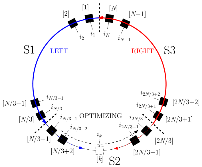
Figure 2: Circular optimization algorithm: the lattice ring of length $N$ is divided into three sectors (S). The single optimization sweep proceeds from site $1$ to site $N$. When a new sector is entered (S2 in the example given in the figure), one builds up the product of transfer matrices for the other two sectors (S1 and S3). At the $k$-th optimization step, before performing the minimization in terms of the generalized eigenvalue problem (6), in order to build up the effective matrices ${\mathbb{H}}_{k}$ and ${\mathbb{N}}_{k}$, one contracts the transfer matrices in the optimizing sector (S2) to the left (right) of the optimizing site with the left (right) truncated SVD, following the order given by the arrows.

In order to guarantee that the number of transfer matrices that have to be multiplied such to form Eq. (15) is sufficiently large, one divides the circular ring into three concatenated sectors of spins (reasonable values for the global system size are $N\gtrsim 10^{2}$). Optimization then starts from one section, say the first one, and proceeds along a fixed direction, say counterclockwise from site $1$ to site $N/3$. Before initiating it, one has to construct the partial effective Hamiltonian and all the required operators corresponding to the two other sectors (second sector from site $N/3+1$ to site $2N/3$, and third sector from site $2N/3+1$ to site $N$) in a SVD-like fashion, following the prescription of Sec. 2.3.1. Then a set of operators for the optimizing section can be constructed by successively adding transfer matrices from the rightmost part of the optimizing section to the left of the operators constructed for the section on the right. After this, the normal optimization procedure can go on, until the border of the optimizing section has been reached, say site $N/3$. At that point, the procedure repeats from the beginning, with the section on the right (from site $N/3+1$ to site $2N/3$) as the new optimizing section. And so on, in a circular way. A pictorial representation of the scheme discussed here is given in Fig. 2.

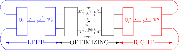
Figure 3: At each optimization step, the matrices ${\mathbb{H}}_{k}$ and ${\mathbb{N}}_{k}$ are built up by contracting the transfer matrices of the three sectors (each line connecting the various blocks indicates a contraction). Due to the truncation in the SVD of the left and right sectors, links $j,j^{\prime}$ and $l,l^{\prime}$ are made up of only $p$ elements. This makes it possible to considerably reduce the computational time for the contractions. The two circles connecting the left and right operators ${\mathbb{U}}$ and ${\mathbb{V}}$ of the left and right sectors stand for diagonal matrices corresponding to the singular values of the two SVD, thus implying $j=j^{\prime}$ and $l=l^{\prime}$. Expliciting the index mapping which leads to the eigenvalue Eq. (6), we get the following component-by-component equation: $[{\mathbb{H}}_{k}]^{i^{\prime}_{k},i_{k}}_{\lambda\rho,\mu\nu}\,[x_{k}]^{i_{k}}_{\mu\nu}=\lambda\,[{\mathbb{N}}_{k}]^{i^{\prime}_{k},i_{k}}_{\lambda\rho,\mu\nu}\,[x_{k}]^{i_{k}}_{\mu\nu}$, where the eigenvector corresponding to minimum eigenvalue $[\bar{x}_{k}]^{i_{k}}_{\mu\nu}:=(A^{[k],i_{k}})_{\mu,\nu}$.

Here we stress that, for each optimization step, once all the required products of transfer matrices are constructed, of course operators relative to the three sectors have to be contracted in a circle (see lines connecting blocks in Fig. 3) so to build up the effective Hamiltonian ${\mathbb{H}}_{k}$ and the effective norm operator ${\mathbb{N}}_{k}$ for a given site $k$. This operation can be performed fast, due to the truncation in the SVD of the left and right sectors. Then one proceeds with the stabilization of the generalized eigenvalue problem (6), following Sec. 2.4, before solving it. Its solution eventually provides the optimized entries of the matrices $A^{[k]}$ in the MPS state at position $k$.

In the following we will use for the first time the proposed MPS algorithm for PBC in order to compute the energy response in a spin ring, when subjected to a change in the boundary conditions (twisted boundary conditions). This permits to quantify the spin stiffness (or analogously the superfluid density in bosonic models). Hereafter we will only be interested in the ground state energies, while expectation values of operators will not be taken into account. This will enable us to obtain reliable results also using MPS descriptions with a relatively small bond link $m\sim 20$.

3 Spin stiffness in the Heisenberg chain

We consider here the spin-$1/2$ Heisenberg model, that is described by the Hamiltonian:

$$\mathcal{H}=J\sum_{j}\left[\frac{1}{2}\left(S^{+}_{j}S^{-}_{j+1}+{\it h.c.}\right)+\Delta S^{z}_{j}S^{z}_{j+1}\right]\,,$$ (21)

where $\sigma^{\alpha}_{j}=2S^{\alpha}_{j}$ ($\alpha=x,y,z$) denote the spin-$1/2$ Pauli matrices on site $j$, $S^{\pm}=S^{x}\pm iS^{y}$ are the raising/lowering spin operators, $J$ is the coupling strength and $\Delta$ is the anisotropy. Hereafter we will set $J=1$ as energy scale, and use units of $\hbar=k_{b}=1$.

In the thermodynamic limit and at zero temperature, this model exhibits a gapless critical phase for $|\Delta|\leq 1$ with quasi-long-range order emerging from power-law decaying correlation functions, while it is gapped and short-ranged for $|\Delta|>1$. The gapless phase is characterized by ballistic transport, which corresponds to a finite spin stiffness $\rho_{s}(\Delta)$ at the thermodynamic limit [18]. This quantity expresses the sensitiveness to a magnetic flux added in the system when PBC are assumed, and can be formally treated by performing a twist in the boundary conditions. Namely, the addition of a flux $\phi$ along the $z$ direction corresponds to take the twisted boundary conditions

$$S^{\pm}_{N+1}=S^{\pm}_{1}e^{\pm i\phi},\qquad S^{z}_{N+1}=S^{z}_{1}\,,$$ (22)

where $N$ denotes the length of the ring. The stiffness is then defined as follows:

$$\rho_{s}:=N\frac{\partial^{2}E_{0}(\phi)}{\partial\phi^{2}}\Big{|}_{\phi=0}\,,$$ (23)

where $E_{0}(\phi)$ is the ground state energy with a magnetic flux of intensity $\phi$. Here we remark that $\rho_{s}$ evaluated with OBC is strictly zero, since with open boundary geometry one can always cancel the effect of the twist by applying suitable gauge conditions to the spins.

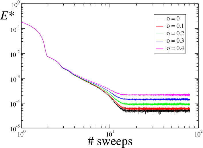
Figure 4: Convergence to the ground-state energy of a spin-$1/2$ Heisenberg chain of length $N=150$ and anisotropy $\Delta=0.5$ with twisted boundary conditions, as a function of the variational steps in the MPS optimization algorithm. Here we used a bond link $m=18$, with truncation indexes $p=50$ and $s=35$; we imposed a random initial guess and performed $80$ sweeps (energies are rescaled over the ground state energy $E_{0}$ with PBC, so that $E^{*}=E-E_{0}+5\times 10^{-5}$. For the sake of clarity, we used a logarithmic scale on the $y$ axis).

By solving the Bethe ansatz equations for model (21), one can show [18] that, at the thermodynamic limit and for $|\Delta|\leq 1$,

$$\rho_{s}(\Delta)=J\frac{\pi\sin(\mu)}{4\mu(\pi-\mu)}\qquad{\rm with}\quad\Delta=\cos(\mu)\,,$$ (24)

while $\rho_{s}(\Delta)$ vanishes for $|\Delta|>1$. The point $|\Delta|=1$ is characterized by a metal-insulator transition between a metallic phase with a finite $\rho_{s}$ and a gapped insulating regime with $\rho_{S}=0$, following a Mott mechanism.

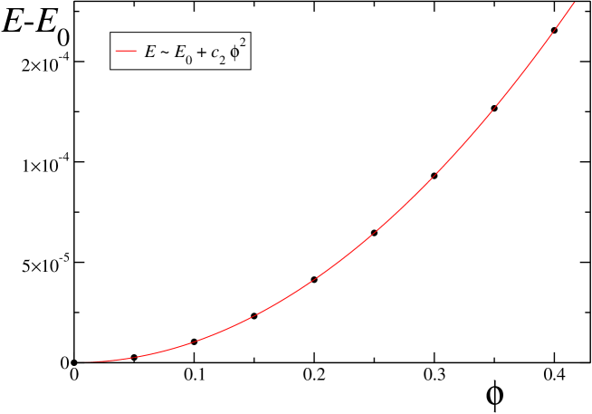
Figure 5: Ground-state energy of a Heisenberg chain of length $N=150$, $\Delta=0.5$, as a function of the twist $\phi$, obtained by averaging the data in Fig. 4 over the last five sweeps. The red curve is a quadratic fit of numerical data (black circles), with $c_{2}\approx 1.03435\times 10^{-3}$.

We employ the MPS algorithm with PBC described above in order to evaluate the stiffness. In Fig. 4 we show the actual system energy at each step of the MPS algorithm. As one can notice, since the algorithm is variational in the energy of the system, the leading behavior of the curve is monotonic decreasing. When the energy is close to its convergence point, fluctuations due to the truncation in the SVD process become evident . Anyway, provided the two truncation parameters $p$ and $s$ are chosen sufficiently large, as it is the case in Fig. 4, an average over the last sweeps is in general sufficient to sweep away all the unwanted fluctuations. This clearly emerges from the averaged converged values of the energy, plotted in Fig. 5 as a function of the twist angle $\phi$ for twisted boundary conditions. Indeed a neat quadratic behavior is visible. We then fitted the curve $E_{0}(\phi)$ with a quadratic law: $E_{0}(\phi)=E_{0}(0)+c_{2}\phi^{2}$ (see the red line), obtaining the prefactor $c_{2}$ which is directly related to the stiffness:

$$\rho_{s}=2Nc_{2}\,.$$ (25)

In the figure we used a bond link $m=18$, which is considerably smaller than the one used in actual simulations performed for OBC (for well optimized codes, $m$ can typically reach values one order of magnitude larger). Nonetheless we should also point out that typically large numbers of $m$ are required for evaluating local observables or correlation functions; on the contrary, here we are only interested in the ground state energies for which large values of $m$ are less crucial. As an example, in the case of the isotropic Heisenberg chain, with $m=18$ we found $E_{0}/N\approx-0.443138$ which is still not far from the thermodynamic limit value obtained from Bethe ansatz calculations $\epsilon=-\ln 2+1/4\approx-0.443147$.

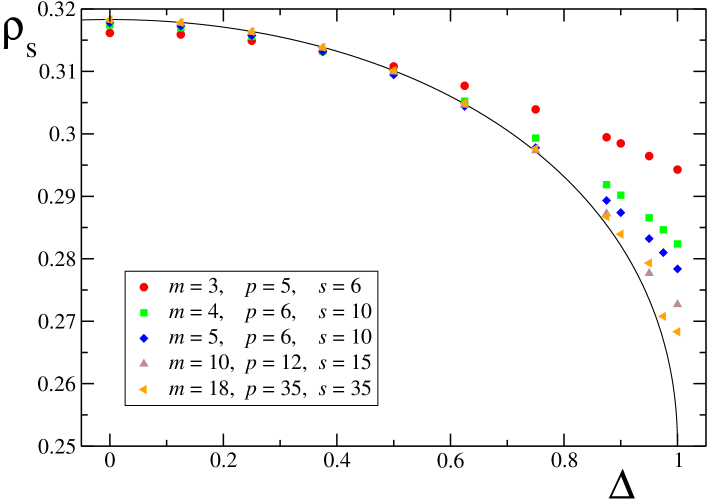
Figure 6: Spin stiffness in the critical phase of the Heisenberg spin-$1/2$ chain, Eq. (21) with $|\Delta|\leq 1$. Symbols are obtained from numerical simulations of a system with $N=180$ sites, for different values of the bond link $m$ (and, accordingly, different values of $p$ and $s$, see the legend). The straight curve is the analytic estimate as obtained from the Bethe ansatz, Eq. (24).

A plot of the spin stiffness (23) as a function of the anisotropy $\Delta$, in the critical phase $|\Delta|\leq 1$ is shown in Fig. 6, where data have been collected for systems of $N=180$ sites. We obtained $\rho_{S}$ as a response in the ground-state energy to a twist in the BCs, using Eq. (25). As it is apparent from the figure, modest values of $m$ are sufficient to attain good accuracies for $\rho_{s}$: for values of the anisotropy sufficiently far from the isotropic limit, at $m=18$ we are able to reach precisions in $\rho_{s}$ of the order $\sim O(10^{-5})$. In particular, the convergence to the exact value at the thermodynamic limit appears to be approximately power-law in $1/m$, with an exponent $\sim 2.5$ as explicitly shown in Fig. 7. We also noted that the dependence of the stiffness on the system size $N$ is negligible on the scale of Fig. 6 for $N\gtrsim 10^{2}$, even if they can become relevant in a comparison with the exact value at the thermodynamic limit, as it is done in Fig. 7.

Special care has to be taken in the region close to the border of the critical zone $\Delta\sim 1$: this requires higher precisions. Moreover, here the convergence of the minimization algorithm becomes much slower (more than one hundred of sweeps are required in order to reach the minimum of energy). The reason is due to the antiferromagnetic character of the Hamiltonian in this regime [12]; this problem could be at least partly overcome by performing a minimization algorithm similar to the one proposed here, but which optimizes two sites at the same time.

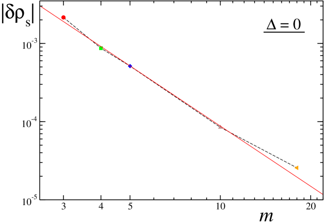
Figure 7: Absolute differences $|\delta\rho_{s}|$ between the stiffness in the Heisenberg model with $N=180$ sites, evaluated with a given bond link dimension $m$, and the exact value at the thermodynamic limit, as given by Eq. (24). The continuous red line denotes a power-law fit of data $|\delta\rho_{s}|\sim m^{-2.56}$. Data shown are for $\Delta=0$.

3.1 Convergence with the truncation parameters

We now discuss the stability of the algorithm with respect to the various approximations introduced for speeding up the PBC problem. Our MPS algorithm for PBC is governed by three control parameters: the size $m$ of the matrices in the MPS representation (1), the two truncation parameters on the singular values of long products of transfer matrices ($p$) and on the effective Hamiltonian ($s$). As we already discussed before and as it is apparent from Fig. 7, the bond link controls the global accuracy of the algorithm. This is analogous to the standard DMRG algorithms, where an increase of $m$ typically produces a converged value of the ground state energy which monotonically decreases towards the exact value. In our case, we found an approximately power-law convergence with $m$ of the stiffness $\rho_{s}$.

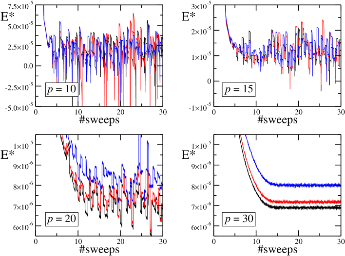
Figure 8: Convergence of the MPS periodic optimization algorithm, as a function of the truncation parameter $p$. The different panels display the ground-state energy per-spin of a spin-$1/2$ Heisenberg chain of length $N=150$ and anisotropy $\Delta=0.5$ with twisted boundary conditions, as a function of the variational steps. Here we fixed the bond link $m=18$, and the index $s=35$ (energies are rescaled such that $E^{*}=E+0.375$). The four panels are for $p=10,\,15,\,20,\,30$. Note that the scale on the $y$ axis of the upper left, the upper right, and the two lower panels are different.

Let us concentrate on the effects of the truncations. We first discuss the convergence of the algorithm with $p$. This parameter expresses the number of singular values that are kept in the SVD representation of the product of transfer matrices belonging to sectors other than the one on which the optimization is running on (see Sec. 2.5 and Fig. 2), and it ranges in the interval $[1,m^{2}]$. Only in the case $p=m^{2}$ no errors are introduced in the SVD representation; any $p<m^{2}$ will introduce further errors in the algorithm. As it is clearly visible from Fig. 8, where in the different panels we show the convergence of the ground state energy for different values of $p$ fixing $m$ and $s$, a value of $p<m^{2}$ introduces non-monotonic fluctuations in correspondence of any change of sector, during the optimization algorithm (therefore with periodicity $1/3$, in units of the number of sweeps). On the contrary, while the algorithm is running in a given sector without changing it, the energy is monotonically decreasing, due to the intrinsic variational character of the optimization. When $p$ is increased, these fluctuations diminish, until they become hardly visible on the scale of the figure for $p\gtrsim m$ (note that the energy scale in the panels of Fig. 8 is different). For example, in the case $m=18$ we obtained quite stable results for $p\gtrsim 30$. We remark that for low values of $p$ ($p=10,\,15$ in the two upper panels of Fig. 8), due to strong fluctuations, we could not even see an increase of the energy with the magnetic flux $\phi$, therefore it was impossible to extract a value for the spin stiffness $\rho_{s}$.

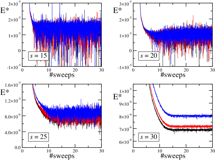
Figure 9: Same as in Fig. 8, but keeping $p=35$ fixed and varying the truncation parameter $s=15,\,20,\,25\,30$. Note that the scale on the $y$ axis of the two upper panels, the lower left and the lower right panel are different.

We finally focus on the convergence with $s$, which quantifies the number of singular values kept in the SVD of the effective Hamiltonian ${\mathbb{H}}_{k}^{\prime}$. It turns out that, as it happens with the other truncation parameter $p$, by increasing $s\in[1,m^{2}]$ we found a decrease of the fluctuations (see Fig. 9). However these fluctuations can be distinguished from the ones due to $p$, since they do not have a definite periodic structure and are random, as a function of the steps in the algorithm. This is because at each variational step one has to construct an effective Hamiltonian. Like for $p$, we found that a value $s\gtrsim m$ is able to reduce such fluctuations such to obtain stable values for the converged energy (in the example of Fig. 9 with $m=18$, we noted that $s\gtrsim 30$ is sufficient to compute $\rho_{s}$).

We point out that the correct evaluation of the susceptibility with respect to $\phi$ in Eq. (23) needs an high degree of convergence of the energy $E(\phi)$. As a matter of fact, fluctuations caused by low values of the truncation parameters may completely hide the small variations of $E$ induced by infinitesimal magnetic fields $\phi$, thus invalidating our procedure for the evaluation of $\rho_{s}$ (as it is visible if the upper panels of Figs. 8, 9). In conclusion, as already stated in Sec. 2.3, for our calculations we required $p,s\gtrsim m$, thus practically worsening the computational requirements of the PBC algorithm to $O(m^{4})$, instead of $O(m^{3})$ as it is claimed in Ref. [13]. On the other hand, in order to give a rather precise estimate of the ground state energy $E(\phi=0)$, it is probably sufficient to take lower values of $p$ (as in the upper left panels of Figs. 8, 9, where the relative error induced by the fluctuations is already $\delta E/E_{0}\sim 10^{-6}$, with $\delta E$ being the size of fluctuations and $E_{0}$ the ground state energy). This also explains why Pippan et al. were able to go to larger values of $m$ ($m\sim 50$) but apparently smaller values of $p$, in order to get the ground state energy of the $s=1$ Heisenberg model with their PBC algorithm [13] .

4 Conclusions

In this paper we presented a variational procedure for numerically finding the ground state of a generically non-translationally invariant one-dimensional Hamiltonian model, which can be accurately written as a suitable MPS. This is constructed starting from the work in Ref. [13], which in turn is an improvement of the variational formulation of DMRG given in [9]. On top of this, we elucidated some technical improvements for stabilizing the code, as detailed in Sec. 2.4, which also reveal useful in the precision measurements of energies that we performed subsequently.

The algorithm globally scales as $O(N\times p\times m^{3})$, where $N$ is the system size, $m$ is the size of each matrix in the MPS representation, while $p$ is the number of singular values that are kept in typical SVD decompositions of transfer matrices (generally, for good performances one has to take $p\sim m$). The accuracy of the algorithm is the same as for the open-boundary case, once the dimension $m$ of the matrices is fixed in both cases (it is therefore also the same as for the original DMRG algorithm, where $m$ is the analogous of the number of states kept for describing each block). We point out that, as typically implemented in good DMRG codes, also in this procedure it is in principle possible to take advantage of some specific symmetries of the Hamiltonian under scrutiny. In particular, Abelian U(1) symmetries can be included [19]. Reasonably, this would admit a computational speedup of up to one order of magnitude, as thoroughly noticed in analogous benchmark MPS codes with open boundary conditions.

We showed how to exploit the possibility to change the boundary conditions on the ring, in order to evaluate the response to a magnetic flux added in the system. This provides the so called stiffness, which acts as order parameter for the critical phase. As an example, we calculated the spin stiffness in the spin-$1/2$ Heisenberg chain and compared it with the analytic predictions. The quantitative analysis of the stiffness, in combination with a study of the solid ordering in strongly correlated systems through structure factor measurements, is of crucial importance in the characterization of the different states of matter which may arise, including elusive ones, such as the supersolid phase [20]. It is worth stressing that our MPS algorithm inherently accesses very large systems, thus directly addressing the system properties in the thermodynamic limit.

Appendix A Working principle of the truncated SVD

Consider first the case in which the $m^{2}\times m^{2}$ matrix $M$ admits exactly $r$ non zero singular eigenvalues with $r\ll p$. This implies that its singular decomposition can be expressed as $M=UDV$ with $U\in{\cal M}_{m^{2}\times r}$, $V\in{\cal M}_{r\times m^{2}}$ isometries, and $D={\cal M}_{r\times r}$ diagonal. Now observe that, given $z$ a vector of $\mathbb{C}^{r}$, $Uz$ is a vector of $\mathbb{C}^{m^{2}}$. Define then the subspace $\mathfrak{A}\subset\mathbb{C}^{m^{2}}$ spanned by these vectors, i.e.,

$$\mathfrak{A}=\mbox{Span}\{Uz:z\in\mathbb{C}^{r}\}\;.$$ (26)

By construction it has dimension $r$ and its orthogonal complement is the left-kernel of $M$ (i.e., it is formed by the vectors of $\mathbb{C}^{m^{2}}$ which nullify when we apply $M$ on their right). Let us then consider a full rank random matrix $x\in{\cal M}_{p\times m^{2}}$ with $p<m^{2}$: by construction its rows $x_{1},x_{2},\cdots,x_{p}$ will span a $p$-dimensional subspace $\mathfrak{B}$ of $\mathbb{C}^{m^{2}}$. Since $r\ll p$, we can assume that $\mathfrak{B}$ will have a non trivial overlap with the subspace $\mathfrak{A}$ (i.e., no non trivial subspace of the latter will be fully disconnected from the former). By the same token we also notice that for $\ell=1,\cdots,p$, the vectors $y_{\ell}=x_{\ell}M$ will in general span a subspace $\mathfrak{C}$ of $\mathbb{C}^{m^{2}}$ of dimension no larger than $r$, which with high probability coincides with the image of $\mathbb{C}^{m^{2}}$ generated via the application of $M$ on the right. Via Gram-Schmidt decomposition we construct now an orthonormal set of row vectors $\{y_{\ell}^{\prime}:\ell=1,\cdots,p\}$ which include such space as a proper subspace: using these vectors as rows for a $p\times m^{2}$ matrix, we thus construct the $y^{\prime}$ matrix of the protocol. Let then $w$ be a generic row vector of $\mathbb{C}^{r}$: by construction $wV$ will belong to the $\mathfrak{C}$ space and could be expressed as $wV=\sum_{\ell}\alpha_{\ell}y_{\ell}^{\prime}$. This yields the identity $V=Vy^{\prime{\dagger}}y^{\prime}$ where $y^{\prime}$ is the $p\times m^{2}$ matrix whose rows are given by the vectors $y_{\ell}^{\prime}$. Now define the $m^{2}\times p$ matrix $Z=My^{\prime{\dagger}}$ and compute its SVD decomposition $Z=\tilde{U}\tilde{D}\tilde{V}$: since by construction we have that $Zy^{\prime}=My^{\prime{\dagger}}y^{\prime}=M$ we can conclude that $M=\tilde{U}\tilde{D}\tilde{V}y^{\prime}$ which allows us to identify $\tilde{D}$ with $D$, $\tilde{U}$ with $U$ and $\tilde{V}y^{\prime}$ with the isometry $V$.

Now consider the case in which $M$ possess $r\ll p$ dominant non zero singular eigenvalues, plus others which are negligible (i.e., they are not null as in the previous case, but can still be neglected when compared with the first $d$ ones). The previous derivation still holds in this case: the main difference being that the approximated eigenvalues obtained from $Z$ will correspond to the real ones with an error which scales as $\epsilon$ (the latter being the relative magnitude of the small singular eigenvalue when compared with the large ones). In this respect, it is worth noticing that the procedure does not really produce the first $p$ largest singular eigenvalues of $M$: however, admitting that $r\ll p$, it will approximately produce the first $r$ largest ones.

References

References

- [1] Bloch I, Dalibard J and Zwerger W, 2008 Rev. Mod. Phys. 80 885
- [2] Greiner M, Mandel O, Esslinger T, Hansch T W and Bloch I, 2002 Nature 415 39
- [3] Kim E and Chan M H W, 2004 Nature 427 225
- [4] White S R, 1992 Phys. Rev. Lett. 69 2863; 1993 Phys. Rev. B 48 10345
- [5] Schollwöck U, 2005 Rev. Mod. Phys. 77 259
- [6] Östlund S and Rommer S, 1995 Phys. Rev. Lett. 75 3537
- [7] Schollwöck U, 2011 Ann. Phys. 326 96
- [8] Rapsch S, Schollwöck U and Zwerger W, 1999 Europhys. Lett. 46 559
- [9] Verstraete F, Porras D and Cirac I J, 2004 Phys. Rev. Lett. 93 227205
- [10] Sandvik A W and Vidal G, 2007 Phys. Rev. Lett. 99 220602
- [11] Shi Q-Q and Zhou H-Q, 2009 J. Phys. A: Math. Theor. 42 272002
- [12] Pirvu B, Verstraete F and Vidal G, 2011 Phys. Rev. B 83, 125104
- [13] Pippan P, White S R and Evertz H G, 2010 Phys. Rev. B 81 081103(R)
- [14] Verstraete F, Murg V and Cirac J I, 2008 Adv. Phys. 57 143
- [15] Cirac J I and Verstraete F, 2009 J. Phys. A: Math. Theor. 42 504004
- [16] Eisert J, Cramer M and Plenio M B, 2010 Rev. Mod. Phys. 82 277
- [17] White S R, 2005 Phys. Rev. B 72 180403(R)
- [18] Shastry B S and Sutherland B, 1990 Phys. Rev. Lett. 65 243
- [19] Silvi P et al., in preparation.
- [20] Rossini D, Giovannetti V and Fazio R, 2011 Phys. Rev. B 83 140411(R)