Thermodynamics of the frustrated one-dimensional spin-$1/2$ Heisenberg ferromagnet in a magnetic field

Abstract

We calculate the low-temperature thermodynamic quantities (magnetization, correlation functions, transverse and longitudinal correlation lengths, spin susceptibility, and specific heat) of the frustrated one-dimensional spin-half $J_{1}$-$J_{2}$ Heisenberg ferromagnet, i.e. for $J_{2}<0.25|J_{1}|$, in an external magnetic field using a second-order Green-function formalism and full diagonalization of finite systems. We determine power-law relations for the field dependence of the position and the height of the maximum of the uniform susceptibility. Considering the specific heat at at low magnetic fields, two maxima in its temperature dependence are found.

I Introduction

Frustrated low-dimensional spin systems have attracted increasing attention.schollwoeck ; Lacroix They represent an ideal playground to study the influence of strong (thermal and quantum) fluctuations on thermodynamic quantities. The one-dimensional (1D) $J_{1}-J_{2}$ Heisenberg model with ferromagnetic nearest-neighbor (NN) coupling $J_{1}$ and antiferromagnetic next-nearest-neighbor (NNN) coupling $J_{2}$ has been studied extensively over the last years, see, e.g., Refs. rastelli, ; bursill, ; tmrg, ; honecker, ; krivnov07, ; krivnov08, ; hiki, ; haertel08, ; zinke09, ; lauchli09, ; sirker2010, ; zinke10, ; sato, . It has been pointed out that this model is an appropriate starting point to describe experimental results for the family of the quasi-1D edge-shared chain cuprates, such as $LiVCuV_{4}$, $LiCu_{2}O_{2}$, $NaCu_{2}O_{2}$, $Li_{2}ZrCuO_{4}$, and $Li_{2}CuO_{2}$. gibson ; matsuda ; gippius ; ender ; drechs1 ; drechs3 ; drechs4 ; park ; drechsQneu ; malek The corresponding Hamiltonian of this system with an external magnetic field is given by

$$H=J_{1}\sum_{\langle i,j\rangle}{\bf S}_{i}{\bf S}_{j}+J_{2}\sum_{[i,j]}{\bf S}_{i}{\bf S}_{j}-h\sum_{i}S_{i}^{z},$$ (1)

where $\langle i,j\rangle$ runs over the NN and $[i,j]$ over the NNN bonds. For the exchange constants we assume $J_{1}<0$ and $J_{2}\geq 0$. In most of these materials quite large values of $J_{2}$ are realized leading to incommensurate spiral in-chain spin correlations at low temperatures. Magnetic field effects can be quite strong,dmitriev ; honecker ; hiki ; lauchli09 ; kolezhuk ; nishimoto in particular, if $J_{2}$ is near the quantum critical point $J_{2}^{c}=|J_{1}|/4$, where the transition between the ferromagnetic and incommensurate spiral ground state takes place. On the other hand, some materials considered as 1D $s=1/2$ ferromagnets, such as the copper salt TMCuC,LW79 ; DRS82 the organic magnets p-NPNNTTN91 ; TKI92 and $\beta$-BBDTA$\cdot$GaBr₄,SGM06 may have a weak frustrating NNN exchange interaction. Moreover, in Refs. malek, and schmitt, $Li_{2}CuO_{2}$ and $Li_{2}ZrCuO_{4}$ were identified as quasi-1D $s=1/2$ frustrated ferromagnets with $J_{2}\approx 0.2|J_{1}|$. Although for $J_{2}<J_{2}^{c}$ the ground state of the model (1) is ferromagnetic, it has been shown recentlyhaertel08 ; haertel10 that the low-temperature thermodynamics is strongly influenced by the frustrating $J_{2}$. Moreover, in Refs. magfeld, and ihle_new, it has been found that for unfrustrated 1D quantum ferromagnets at weak magnetic fields the specific heat exhibits an additional low-temperature maximum indicating a separation of two energy scales. Interestingly, this field-induced low-temperature maximum appears only in 1D systems and for the small spin quantum numbers, $s=1/2$ and $s=1$.magfeld ; ihle_new Therefore, it can be considered as a characteristic feature of 1D quantum ferromagnets.

In this paper we consider the interplay between frustration and magnetic field in 1D $s=1/2$ ferromagnets, i.e. we study the model (1) in the parameter regime $J_{2}<|J_{1}|/4$, where the ferromagnetic ground state is realized. In difference to previous investigations,magfeld ; ihle_new neither the Bethe ansatz nor the quantum Monte Carlo method can be used. Hence, we employ (i) a second-order Green-function method (GFM) for infinite chains and (ii) exact diagonalization (ED) of finite chains with $N=16$ and $N=20$ spins imposing periodic boundary conditions to calculate thermodynamic properties. It has been shown in Refs. haertel08, ; magfeld, and ihle_new, that both techniques may provide reliable results for the problem under consideration.

The Green-function technique for Heisenberg spin systems used here was initially introduced by Kondo and Yamaij in a rotation-invariant formulation.kondo It has been further developed and successfully applied to low-dimensional quantum systems over the last decade.haertel08 ; magfeld ; ihle_new ; rgm_new ; antsyg The specific version of the method appropriate for spin systems in a magnetic field was developed in Ref. ihle_new, .

The paper is organized as follows. In Sec. II we illustrate the main features of the GFM. In Sec. III we present our results for the magnetization, the susceptibility, the spin-spin correlation functions, the correlation length, and the specific heat. A summary of our results is given in Sec. IV.

II Second-order Green-function theory

To calculate the longitudinal and transverse spin correlation functions and other thermodynamic quantities, we use two-time retarded commutator Green functions.elk First we determine the longitudinal spin correlation functions from the Green function $\langle\langle S_{q}^{z};S_{-q}^{z}\rangle\rangle_{\omega}=-\chi_{q}^{zz}\left(\omega\right)$, where $\chi_{q}^{zz}\left(\omega\right)$ is the longitudinal dynamic spin susceptibility. The equation of motion reads

$$\omega^{2}\langle\langle S_{q}^{z};S_{-q}^{z}\rangle\rangle_{\omega} =M_{q}^{zz}+\langle\langle-\ddot{S}_{q}^{z};S_{-q}^{z}\rangle\rangle_{\omega},$$ (2)

$$M_{q}^{zz} =-2\sum_{n=1,2}J_{n}C_{n}^{-+}\left(1-\cos nq\right),$$ (3)

where $C_{n}^{-+}=\langle S_{0}^{-}S_{n}^{+}\rangle$. To approximate the second derivative $-\ddot{S}_{q}^{z}$ we use a decoupling scheme proposed in Refs. kondo, ; rgm_new, ; magfeld, ; antsyg, ; ihle_new, which reads

$$S_{i}^{z}S_{j}^{+}S_{k}^{-} =\alpha_{jk}^{zz}\langle S_{j}^{+}S_{k}^{-}\rangle S_{i}^{z},$$ (4)

where for the vertex parameters $\alpha_{jk}^{zz}$ we assume $\alpha_{jk}^{zz}\equiv\alpha_{1}^{zz}$ if $j,k$ are NN, and $\alpha_{jk}^{zz}\equiv\alpha_{2}^{zz}$ otherwise. We obtain $-\ddot{S}_{q}^{z}=(\omega_{q}^{zz})^{2}S_{q}^{z}$ and

$$\chi_{q}^{zz}=-\langle\langle S_{q}^{z};S_{-q}^{z}\rangle\rangle_{\omega}=\frac{M_{q}^{zz}}{(\omega_{q}^{zz})^{2}-\omega^{2}}$$ (5)

with

$$(\omega_{q}^{zz})^{2}= \sum_{n,m(=1,2)}J_{n}J_{m}(1-\cos nq)$$

$$\qquad\times\left[K_{n,m}^{zz}+4\alpha_{n}^{zz}C_{n}^{-+}(1-\cos mq)\right],$$

where $K_{n,n}^{zz}=1+2(\alpha_{2}^{zz}C_{2n}^{-+}-3\alpha_{n}^{zz}C_{n}^{-+})$, $K_{1,2}^{zz}=2(\alpha_{2}^{zz}C_{3}^{-+}-\alpha_{1}^{zz}C_{1}^{-+})$, and $K_{2,1}^{zz}=K_{1,2}^{zz}+4(\alpha_{1}^{zz}C_{1}^{-+}-\alpha_{2}^{zz}C_{2}^{-+})$. Applying the spectral theoremelk to the Green function (5), the longitudinal correlation functions of arbitrary range $n$, $C_{n}^{zz}=\langle S_{0}^{z}S_{n}^{z}\rangle$, can be calculated bymagfeld ; ihle_new

$$C_{n}^{zz} =\frac{1}{N}\sum_{q\neq 0}C_{q}^{zz}e^{iqn}+\langle S^{z}\rangle^{2},$$ (7)

$$C_{q}^{zz} =\langle S_{-q}^{z}S_{q}^{z}\rangle=\frac{M_{q}^{zz}}{2\omega_{q}^{zz}}\left[1+2n(\omega_{q}^{zz})\right],$$ (8)

where $n(\omega_{q}^{zz})=\left(e^{\omega_{q}^{zz}/T}-1\right)^{-1}$ is the Bose function. For $n=0$, we get the sum rule $C_{0}^{zz}=1/4$. As shown in Ref. ihle_new, , the isothermal and the uniform static Kubo susceptibility $\chi_{0}^{zz}$ agree at arbitrary fields and temperatures. Using Eqs. (3), (5), and (II) we get the relation

$$\frac{\partial\langle S^{z}\rangle}{\partial h} =-\frac{2}{\Delta^{zz}}\sum_{n=1,2}n^{2}J_{n}C_{n}^{-+},$$ (9)

$$\Delta^{zz} =\sum_{n,m(=1,2)}n^{2}J_{n}J_{m}K_{n,m}^{zz}.$$ (10)

Among others, Eq. (9) can be used to determine the vertex parameters.

To calculate the transverse correlation functions, we use the Green function $\langle\langle S_{q}^{+};S_{-q}^{-}\rangle\rangle_{\omega}=-\chi_{q}^{+-}\left(\omega\right)$, where $\chi_{q}^{+-}\left(\omega\right)$ is the transverse dynamic spin susceptibility. Here the equations of motion read

$$\omega\langle\langle S_{q}^{+};S_{-q}^{-}\rangle\rangle_{\omega} =2\langle S^{z}\rangle+\langle\langle i\dot{S}_{q}^{+};S_{-q}^{-}\rangle\rangle_{\omega},$$ (11)

$$\omega\langle\langle i\dot{S}_{q}^{+};S_{-q}^{-}\rangle\rangle_{\omega} =M_{q}^{+-}+\omega\langle\langle-\ddot{S}_{q}^{+};S_{-q}^{-}\rangle\rangle_{\omega}.$$ (12)

The moment $M_{q}^{+-}=\langle\left[i\dot{S}_{q}^{+},S_{-q}^{-}\right]\rangle$ is given by

$$M_{q}^{+-}=-4\sum_{n=1,2}J_{n}C_{n}\left(1-\cos nq\right)+2h\langle S^{z}\rangle,$$ (13)

where $C_{n}=\frac{1}{2}C_{n}^{-+}+C_{n}^{zz}$. In $-\ddot{S}_{q}^{+}$ we decouple the products of three operators as

$$S_{i}^{-}S_{j}^{+}S_{k}^{+}=\alpha_{i,j}^{+-}\langle S_{i}^{-}S_{j}^{+}\rangle S_{k}^{+}+\alpha_{i,k}^{+-}\langle S_{i}^{-}S_{k}^{+}\rangle S_{j}^{+},$$ (14)

where again for the vertex parameters $\alpha_{i,j}^{+-}$ we assume $\alpha_{jk}^{+-}\equiv\alpha_{1}^{+-}$ if $j,k$ are NN, and $\alpha_{jk}^{+-}\equiv\alpha_{2}^{+-}$ otherwise. We obtain

$$-\ddot{S}_{q}^{+}=\left[(\omega_{q}^{+-})^{2}-h^{2}\right]S_{q}^{+}+2hi\dot{S}_{q}^{+}$$ (15)

with

$$(\omega_{q}^{+-})^{2}= \sum_{n,m(=1,2)}J_{n}J_{m}(1-\cos nq)$$

$$\qquad\times\left[K_{n,m}^{+-}+4\alpha_{n}^{+-}C_{n}(1-\cos mq)\right],$$

where $K_{n,n}^{+-}=1+2(\alpha_{2}^{+-}C_{2n}-3\alpha_{n}^{+-}C_{n})$, $K_{1,2}^{+-}=2(\alpha_{2}^{+-}C_{3}-\alpha_{1}^{+-}C_{1})$, and $K_{2,1}^{+-}=K_{1,2}^{+-}+4(\alpha_{1}^{+-}C_{1}-\alpha_{2}^{+-}C_{2})$. Finally, the resulting Green functions are

$$\langle\langle S_{q}^{+};S_{-q}^{-}\rangle\rangle_{\omega} =\sum_{i=1,2}\frac{A_{qi}}{\omega-\omega_{qi}},$$ (17)

$$\langle\langle i\dot{S}_{q}^{+};S_{-q}^{-}\rangle\rangle_{\omega} =\sum_{i=1,2}\frac{\omega_{qi}A_{qi}}{\omega-\omega_{qi}},$$ (18)

where

$$\omega_{q1,2}=h\pm\omega_{q}^{+-},$$ (19)

$$A_{q1,2}=\langle S^{z}\rangle\pm\frac{1}{2\omega_{q}^{+-}}\left(M_{q}^{+-}-2h\langle S^{z}\rangle\right).$$ (20)

As argued in Ref. ihle_new, , a divergence in the transverse static spin susceptibility $\chi_{q}^{+-}(\omega=0)$, which signals a phase transition, could appear if $\omega_{q_{c}2}=0$, i.e., $\omega_{q_{c}}^{+-}=h$. Since for nonzero fields, the Heisenberg ferromagnet (1) does not describe a phase transition, $\chi_{q}^{+-}(\omega=0)$ has to be finite at all $q$. To ensure this, we require $A_{q_{c}2}=0$ which results in the regularity condition

$$h\langle S^{z}\rangle=-2\sum_{n=1,2}J_{n}C_{n}\left(1-\cos nq_{c}\right).$$ (21)

Following Refs. ihle_new, and antsyg, , we assume this condition to be valid also for larger fields, where $h>\omega_{q}^{+-}$ for all $q$, to guarantee the continuity of all quantities.
Applying the spectral theorem to the Green functions (17) and (18), we obtain the transverse correlation functions $C_{n}^{-+}=\langle S_{0}^{-}S_{n}^{+}\rangle=\frac{1}{N}\sum_{q}C_{q}^{-+}e^{iqn}$ and $\tilde{C}_{n}^{-+}=\langle S_{0}^{-}i\dot{S}_{n}^{+}\rangle=\frac{1}{N}\sum_{q}\tilde{C}_{q}^{-+}e^{iqn}$ of arbitrary range $n$ with the structure factors

$$C_{q}^{-+}=\sum_{i=1,2}A_{qi}n(\omega_{qi}),\tilde{C}_{q}^{-+}=\sum_{i=1,2}\omega_{qi}A_{qi}n(\omega_{qi}).$$ (22)

From the $s=1/2$ operator identity $S_{i}^{-}S_{i}^{+}+S_{i}^{z}=\frac{1}{2}$ we find the sum rule

$$\langle S^{z}\rangle=\frac{1}{2}-C_{0}^{-+}.$$ (23)

Following Ref. ihle_new, , a higher-derivative sum rule can be obtained by multiplying $S_{i}^{-}$ by $i\dot{S}_{i}^{+}$ and expressing the expectation value by Eq. (22),

$$-\frac{1}{N}\sum_{q}\omega_{q}^{+-}\sum_{i=1,2}(-1)^{i}A_{qi}\;n(\omega_{qi})$$

$$=2\sum_{n=1,2}J_{n}\left(C_{n}-\frac{1}{2}\langle S^{z}\rangle\right).$$ (24)

Figure 1: Magnetization for $J_{2}=0,0.1,0.15$ (from top to bottom) and $h=0.005,0.03,0.1$ versus temperature [GFM - lines; ED ($N=20$) - open symbols].

Considering the ground state, at $T=0$, we have the exact results

$$C_{n}^{-+}\left(0\right)=0,\qquad C_{n}^{zz}\left(0\right)=\frac{1}{4},\qquad\langle S^{z}\rangle\left(0\right)=\frac{1}{2}.$$ (25)

Here $C_{n}^{-+}\left(0\right)$ is independent of $n$, so $A_{q1,2}\left(0\right)$ must be independent of $q$. This requires $K_{n,m}\left(0\right)=0$ which yields $\alpha_{1,2}^{+-}(0)=1$. Concerning the zero-temperature values of $\alpha_{1,2}^{zz}$, they can be determined only in the limit $T\to 0$ since Eqs. (7) and (8) for $C_{n}^{zz}$ contain $M_{q}^{zz}$ with $\lim_{T\to 0}M_{q}^{zz}=0$. To evaluate the thermodynamic properties, the correlators $C_{n}^{zz}$ and $C_{n}^{-+}$ for $n\neq 0$ are calculated by Eqs. (7) and (22), whereas $\langle S^{z}\rangle$ and the vertex parameters $\alpha_{1,2}^{+-}$ and $\alpha_{1,2}^{zz}$ are determined from the sum rules [Eqs. (23), (II), and $C_{0}^{zz}=1/4$], the equality (9) and the regularity condition (21).

III Results and Discussion

In what follows we put $|J_{1}|=1$. The coupled system of nonlinear algebraic self-consistency equations derived in Sec. II is solved numerically using Broyden’s method,NR2 which yields the solutions with a relative error of about $10^{-7}$ on the average. The momentum sums for $N\to\infty$ are transformed to integrals which are evaluated by Gaussian integration. Tracing the GFM solution to very low temperature we find it to become less trustworthy for $J_{2}$ approaching $J_{2}=0.25$. Therefore, below we will present GFM results for $J_{2}\leq 0.2$ only. On the other hand, there is no restriction with respect to the value of $J_{2}$ for the ED calculations.

We restrict our discussion to magnetic fields $h\lesssim 0.1$. For typical values of the exchange parameters of the order of 10 meVdrechs1 ; drechs3 that corresponds to values of the magnetic field $H\lesssim 10$T mostly used in experiments.

III.1 Magnetization

First we consider the magnetization $\langle S^{z}\rangle$, see Fig. 1. Obviously, at fixed magnetic field the frustration reduces the magnetization for $T>0$, whereas an increase of the magnetic field at fixed $J_{2}$ leads to an increase of $\langle S^{z}\rangle$. The GFM and ED data agree well with each other.

Figure 2: Magnetic susceptibility $\chi$ versus temperature $T$ (GFM - lines; ED $N=20$ - filled circles; ED $N=16$ - open triangles) for (a) $J_{2}=0.05$ and (b) $J_{2}=0.15$ with $h=0.01,0.05,0.08$, from top to bottom. The insets show the position and height of the maximum obtained by GFM (filled squares) and ED $N=20$ (open circles) as well as the fit by the power law (lines), see Eq. (26).

III.2 Magnetic susceptibility

The uniform magnetic susceptibility $\chi=\partial\langle S^{z}\rangle/\partial h$ at zero field diverges at $T=0$ indicating the ferromagnetic phase transition. Based on GFM data it was found in Ref. haertel08, that $\displaystyle\lim_{T\rightarrow 0}\chi T^{2}=(1-4J_{2})/24$. (Note that for $J_{2}=0$ the rigorous Bethe-ansatz resultyamada is reproduced.) In finite magnetic fields one has $\displaystyle\lim_{T\rightarrow 0}\chi=0$, and $\chi$ exhibits a maximum. The position $T_{max}^{\chi}$ and the height $\chi_{max}$ of this maximum depend on the strength of the magnetic field $h$ and also on the frustration $J_{2}$.

The field dependence of the position of the susceptibility maximum was discussed, for example, in connection with experiments on La_0.91Mn_0.95O₃.MRG00 For the unfrustrated ferromagnet ($J_{2}=0$) it was shownihle_new ; magfeld ; sznaid that interestingly power laws for the field dependence of $T_{max}^{\chi}$ and $\chi_{max}$ are valid, namely

$$T_{max}^{\chi}=ah^{\gamma}\;,\qquad\chi_{max}=bh^{\beta}.$$ (26)

We mention that our analysis of the susceptibility data reproduces the results reported in Refs. magfeld, ; ihle_new, for $J_{2}=0$. Note that $a,\gamma,b$, and $\beta$ depend on the spin quantum number $s$ and dimensionality $D$.magfeld ; ihle_new

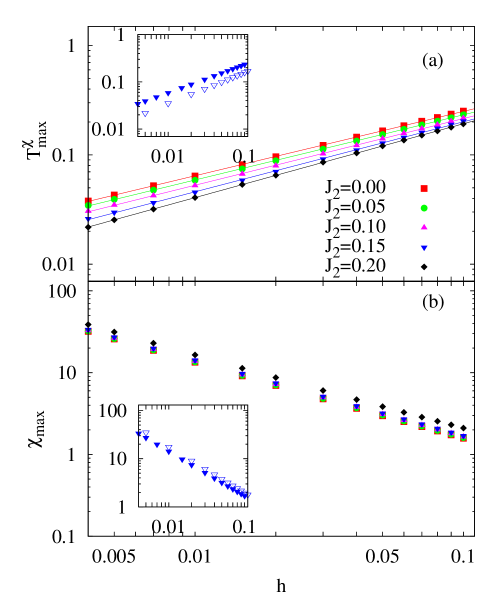
Figure 3: Field dependence of (a) the position $T_{max}^{\chi}$ and (b) the height $\chi_{max}$ of the maximum of the magnetic susceptibility obtained by GFM (main panels). The lines in the upper panel show the fits by the power law Eq. (26). In the insets the GFM results (filled triangles) and the corresponding ED data for $N=20$ (open triangles) are compared for $J_{2}=0.15$.

Figure 4: Coefficients (a) $\gamma$ and (b) $a$ of the power law $T_{max}^{\chi}=ah^{\gamma}$ in dependence on the frustration $J_{2}$ obtained by GFM and ED (N=16,20). For $J_{2}=0$ also the Bethe-ansatz resultmagfeld is shown.

Figure 5: Coefficients (a) $\beta$ and (b) $b$ of the power law $\chi_{max}=bh^{\beta}$ in dependence on the frustration $J_{2}$ obtained by GFM and ED (N=16,20). For $J_{2}=0$ also the Bethe-ansatz resultmagfeld is shown.

Now we discuss the susceptibility for the frustrated ferromagnet, see Fig. 2. The behavior is similar to the unfrustrated case, i.e. for a fixed $J_{2}$, the position $T_{max}^{\chi}$ of the maximum increases and the height $\chi_{max}$ decreases with increasing field. For a fixed $h$ with increasing of frustration $J_{2}$, the position of the maximum is slightly shifted to lower temperatures, whereas the height is almost fixed for $J_{2}<0.2$. The ED and GFM data match to each other reasonably well except the noticeable difference near the maximum.

Next we discuss the validity of the power law (26) for finite frustration $J_{2}>0$, see insets of Fig. 2. We find that the GFM as well as the ED data are well described by the power law (26) in the whole range of frustration (i.e. $J_{2}\leq 0.2$ for the GFM and $J_{2}<0.25$ for the ED), see the log-log plots of $T_{max}^{\chi}$ and $\chi_{max}$ in Fig. 3. The influence of frustration is quite weak. To obtain the dependences of the coefficients on the frustration $J_{2}$ we fit the position and the height of the maximum by the power law using the data points shown in Fig. 3. The variation of the coefficients $a$, $\gamma$, $b$, and $\beta$ with $J_{2}$ shown in Figs. 4 and 5 is weak for $J_{2}<0.2$ (note the enlarged scale in Figs. 4 and 5). The difference between the ED and GFM data may be attributed to finite-size effects. Obviously, the ED for $N=20$ match better to the GFM data than the ED data for $N=16$ (except for the parameter $a$ at larger $J_{2}$.) For comparison, we have also shown the exact Bethe-ansatz resultsmagfeld for $J_{2}=0$. The GFM data agree well with the exact data, except for the parameter $a$, where the difference is about $23\%$. For $J_{2}\gtrsim 0.2$, we have only ED data. In this parameter region the finite size-effects are very small, and there is a noticeable change of the coefficients $a$, $\gamma$, and $\beta$ with frustration.

III.3 Correlation functions

Next we consider the spin-spin correlation functions depicted in Fig. 6. Obviously, the GFM results for the correlation functions agree quite well with the ED data.

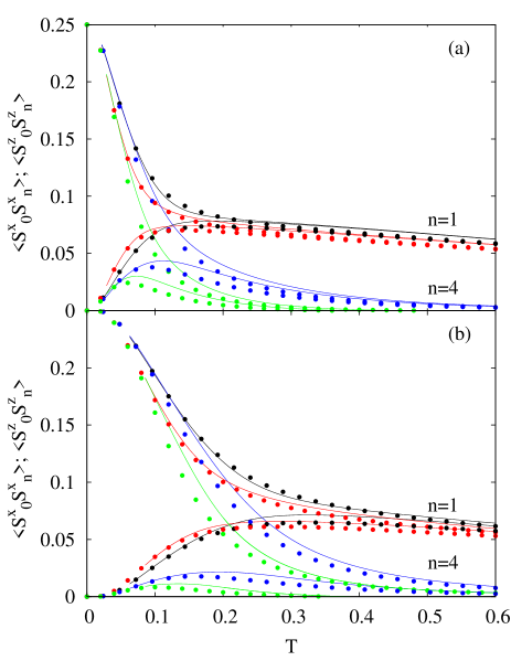
Figure 6: Spin-spin correlation functions $\langle S_{0}^{z}S_{n}^{z}\rangle$ and $\langle S_{0}^{x}S_{n}^{x}\rangle$ for $n=1$ and $n=4$ for (a) $h=0.03$ and (b) $h=0.1$ (GFM - lines, ED data for $N=20$ - symbols, black lines/symbols: $J_{2}=0$, $n=1$; red lines/symbols: $J_{2}=0.15$, $n=1$; blue lines/symbols: $J_{2}=0$, $n=4$; green lines/symbols: $J_{2}=0.15$, $n=4$).

Due to the magnetic field in $z$-direction we have a different behavior of the longitudinal correlation functions $\langle S_{0}^{z}S_{n}^{z}\rangle$ and the transverse ones $\langle S_{0}^{x}S_{n}^{x}\rangle=\langle S_{0}^{y}S_{n}^{y}\rangle$. At $T\gg h$ this difference disappears. At low temperatures the transverse correlation functions exhibit a maximum, where its position and height depend on the spin-spin separation $n$, the frustration $J_{2}$, and the magnetic field $h$. As expected, frustration suppresses the correlations, i.e., there is a faster decay of the correlation functions with increasing $J_{2}$. The strength of the magnetic field at fixed $J_{2}$ influences the correlation functions at low temperatures only. Increasing of $h$ yields a shift of the maximum in $\langle S_{0}^{x}S_{n}^{x}\rangle$ to higher temperatures and a slower decay of the correlation functions with $T$.

III.4 Correlation length

Figure 7: (a) Transverse and (b) longitudinal correlation lengths in dependence on the temperature for frustration parameters $J_{2}=0,0.1,0.15$ (from top to bottom) and for various values of the magnetic field.

Within the GFM formalism we are able to calculate the correlation length.kondo ; haertel08 ; ihle_new Due to the field-induced anisotropy we have again to distinguish between the longitudinal correlation length $\xi^{+-}$ and the transverse correlation length $\xi^{zz}$. Both quantities can be obtained by expanding the static susceptibilitiesihle_new $\chi_{q}^{\nu\mu}$, $\nu\mu=+-,zz$, around the magnetic wave vector ${\bf q}=0$ which leads to $\chi_{q}^{\nu\mu}=\chi_{0}^{\nu\mu}/\left\{1+\left(\xi^{\nu\mu}\right)^{2}q^{2}\right\}$. We obtain

$$\left(\xi^{+-}\right)^{2}=\frac{-J_{1}C_{1}-4J_{2}C_{2}}{\langle S^{z}\rangle h}-\frac{\Delta^{+-}}{2h^{2}}\;,$$ (27)

$$\Delta^{+-}=\sum_{n,m(=1,2)}n^{2}J_{n}J_{m}K_{n,m}^{+-}$$ (28)

and

$$\left(\xi^{zz}\right)^{2}=\frac{2\left(J_{1}+4J_{2}\right)\left(J_{1}\alpha_{1}^{zz}C_{1}^{-+}+4J_{2}\alpha_{2}^{zz}C_{2}^{-+}\right)}{\Delta^{zz}},$$ (29)

where $\Delta^{zz}$ is given by Eq. (9). As found in Ref. ihle_new, , the transverse and longitudinal correlation lengths have qualitatively different temperature dependences at $J_{2}=0$. In particular, the longitudinal correlation length $\xi^{zz}$ reveals an anomaly, namely a shoulder at $T\sim 0.4$ appearing at low magnetic fields, cf. also Fig. 7(b).

Considering the transverse correlation length $\xi^{+-}$ shown in Fig. 7(a), the magnetic field cuts off the divergence of the zero-field correlation length at $T=0$ (cf. Ref. haertel08, ). This is related to the absence of the $T=0$ phase transition if $h>0$. From Eq. (27) we find $\xi^{+-}(T=0)=\sqrt{\frac{0.5-2J_{2}}{h}}$, i.e., at low temperatures the transverse correlation length increases as $h^{-1/2}$ for $h\to 0$, and it decreases with increasing frustration according to $(1-4J_{2})^{1/2}$. At temperatures larger than the magnetic field the dependence on the field strength becomes weak. As already discussed for the correlation functions, at those temperatures both correlation lengths $\xi^{+-}$ and $\xi^{zz}$ approach each other indicating that the magnetic field becomes irrelevant. On the other hand, the decrease in $\xi^{+-}$ and $\xi^{zz}$ with increasing frustration is observed in the whole temperature range shown. At low temperatures $T\lesssim h$ we find $\xi^{zz}<\xi^{+-}$. At very low temperatures this relation might be reversed. Unfortunately, the GFM does not allow here a conclusive statement on $\xi^{zz}$ as $T\to 0$, since in Eq. (29) for $\xi^{zz}$ both the nominator and denominator go to zero for $T\to 0$ leading to numerical uncertainties.

Figure 8: Specific heat for (a) $J_{2}=0.05$ and (b) $J_{2}=0.15$ with $h=0.005,0.03,0.05,0.08,0.1$, from bottom to top (lines - GFM; symbols - ED for $N=20$).

III.5 Specific heat

Let us first recapitulate some relevant results on the specific heat $C(T)=\partial u/\partial T$ with $u=\langle H\rangle/N=J_{1}\left(C_{1}^{-+}+C_{1}^{zz}\right)+J_{2}\left(C_{2}^{-+}+C_{2}^{zz}\right)-h\langle S^{z}\rangle$ from previous investigations.magfeld ; haertel08 ; tmrg ; ihle_new For the unfrustrated 1D $s=1/2$ ferromagnet at $h=0$ the specific heat shows a broad maximum at $T\sim 0.35$, see, e.g., Refs. magfeld, ; haertel08, , and tmrg, . In a weak magnetic field $h<h^{*}$ a double-maximum structure appears. For the field $h^{*}$ below which the additional low-temperature maximum appears, a Bethe-ansatz analysis gives $h^{*}=0.008$, see Ref. magfeld, , whereas the GFM yields $h^{*}\approx 0.07$.magfeld ; ihle_new On the other hand, for the $J_{1}$-$J_{2}$ model in zero field also a double-maximum structure in $C(T)$ was found. In this case it is induced by frustration, and it appears within the GFM for $J_{2}>0.16$.haertel08 Moreover, it was found in Ref. haertel08, that, although the existence of an additional low-temperature maximum can be detected by GFM and ED, its position and height are strongly size dependent, if the maximum is located at very low temperatures.

Our results for the specific heat of the frustrated ferromagnet in a magnetic field are shown in Fig. 8. Analogously to Refs. magfeld, and ihle_new, , a double-maximum structure is found for small field strengths. An increase of the magnetic field shifts the additional low-temperature maximum to higher temperatures and increases its height. At a sufficiently high field strength $h>h^{*}$ the typical broad maximum of the pure ferromagnet at zero field vanishes, since the low-temperature maximum spreads into the region of the former broad maximum. Although the GFM and the ED data for the specific heat differ quantitatively, the above mentioned qualitative behavior is found by both methods., cf. also the discussion in Refs. haertel08, ; magfeld, and ihle_new, . Recalling that for the unfrustrated ferromagnet the double-maximum structure disappears for $h>h^{*}\approx 0.07$ ($h>h^{*}\approx 0.008$) calculated by GFM (ED), cf. Ref. magfeld, , it can be seen in Fig. 8(b) that $h^{*}$ is shifted to higher values due to frustration. Thus, in Fig. 8(b) at $J_{2}=0.15$, the double-maximum structure is still visible in the GFM data at $h=0.08$ and in the ED data at $h=0.03$.

Figure 9: (a) Coefficients $\rho$ and $r$ of the power law $T_{max,1}^{C}=rh^{\rho}$ in dependence on the frustration parameter $J_{2}$ obtained by GFM. For comparison the Bethe-ansatz results are shown for $J_{2}=0$. (b) Coefficients $\delta$ and $d$ of the power law $C_{max,1}=dh^{\delta}$ in dependence on the frustration parameter $J_{2}$ obtained by GFM. For comparison the Bethe-ansatz results are shown for $J_{2}=0$.

As pointed out in Refs. magfeld, and ihle_new, , for $J_{2}=0$ the position and the height of the additional low-temperature maximum follow a power law

$$T_{max,1}^{C}=rh^{\rho}\;,\qquad C_{max,1}=dh^{\delta}.$$ (30)

To determine the coefficients $r$, $\rho$, $d$, and $\delta$ in dependence on the frustration $J_{2}$ we follow Ref. ihle_new, and fit the position and the height of the low-temperature maximum at low fields, $h=0.001-0.01$ in steps of $0.001$, by the power laws of Eq. (30). For these values of the magnetic field, the ED maximum in $C(T)$ quite strongly depends on the size $N$. Therefore, in Fig. 9 we present the GFM results only. It is obvious that up to $J_{2}\sim 0.15$ all coefficients depend weakly on $J_{2}$. Only beyond $J_{2}\sim 0.15$ the coefficients $r$ and $\rho$ increase noticeably.

Let us finally comment the obvious differences in the GFM and ED data for the specific heat, see Fig. 8. The GFM used here and in many previous papershaertel08 ; magfeld ; ihle_new ; haertel10 ; kondo ; rgm_new ; antsyg is a quite universal analytical method which, as a rule, cannot yield quantitatively highly accurate data. On the other hand, the accuracy of the ED data is also limited at low temperatures due to significant finite-size effects, see, e.g., the discussion in Ref. haertel08, . In cases where other accurate methods (for instance the quantum Monte Carlo method which is applicable to unfrustrated quantum spin systems, see e.g. Ref. ihle_new, ) are available, it was found that GFM results for the specific heat at low temperatures show quite large quantitative differences to precise data, whereas other quantities, such as the susceptibility, are in better agreement. However, it has been demonstrated that both the GFM and the ED in general yield qualitatively correct results also for the specific heat.haertel08 ; ihle_new In particular, the existence of the additional low-temperature maximum in the specific heat at weak magnetic fields discussed in this section was confirmed by a Bethe-ansatz analysismagfeld as well as a quantum Monte Carlo calculationihle_new for the unfrustrated 1D s=1/2 ferromagnet, where both methods are applicable. Hence, we argue that the existence of the additional low-temperature maximum in the specific heat is not questioned, however, quanitative statements have to be taken with caution.

IV Summary

In this paper we use exact diagonalization of finite chains and a second-order Green’s function method to study the influence of a frustrating next-nearest-neighbor coupling $J_{2}$ on low-temperature thermodynamic quantities, such as magnetization, correlation functions, transverse and longitudinal correlation lengths, spin susceptibility, and specific heat of the 1D $s=1/2$ $J_{1}$-$J_{2}$ Heisenberg ferromagnet in a magnetic field $h$. We consider $J_{2}<0.25|J_{1}|$, i.e., the ground state of the model is ferromagnetic, but the low-temperature thermodynamics is strongly influenced by the frustrating $J_{2}$. The results of both methods are in good overall agreement.

The position $T_{max}^{\chi}$ and the height $\chi_{max}$ of the maximum of the uniform susceptibility appearing in finite magnetic fields can be described by the power laws $T_{max}^{\chi}=ah^{\gamma}$ and $\chi_{max}=bh^{\beta}$, where the coefficients $a$, $\gamma$, $b$, and $\beta$ weakly depend on $J_{2}$. The double-maximum structure of the specific heat $C(T)$ found for $J_{2}=0$ at low fieldsmagfeld ; ihle_new occurs also for $J_{2}\neq 0$. The field strength at which this structure vanishes is slightly increasing with frustration. The position and the height of the additional low-field low-temperature maximum in $C(T)$ in dependence on the field strength can be also described by power laws.

Acknowledgment
This work was supported by the DFG (project RI615/16-1). The full diagonalization of finite spin systems was done using J. Schulenburg’s spinpack.

References

- (1) Quantum Magnetism, eds. U. Schollwöck, J. Richter, D. J. J. Farnell, and R. F. Bishop, Lecture Notes in Physics 645 (Springer-Verlag, Berlin, 2004).
- (2) Introduction to Frustrated Magnetism, eds. C. Lacroix, P. Mendels and F. Mila, Springer Series in Solid-State Sciences 164 (Springer-Verlag, Berlin, 2011).
- (3) A. Pimpinelli, E. Rastelli, and A. Tassi, J. Phys.: Condens. Matter 1, 7941 (1989).
- (4) R. Bursill, G.A. Gehring, D.J.J. Farnell, J.B. Parkinson, T. Xiang, and C. Zeng, J. Phys.: Condens. Matter 7, 8605 (1995).
- (5) H. T. Lu, Y. J. Wang, Shaojin Qin, and T. Xiang, Phys. Rev. B 74, 134425 (2006).
- (6) F. Heidrich-Meisner, A. Honecker, and T. Vekua, Phys. Rev. B 74 020403(R) (2006).
- (7) D.V. Dmitriev, V.Ya. Krivnov, and J. Richter, Phys. Rev. B 75, 014424 (2007).
- (8) D.V. Dmitriev and V.Ya. Krivnov, Phys. Rev. B 77, 024401 (2008).
- (9) T. Hikihara, T. Momoi , A. Furusaki, and H. Kawamura Phys. Rev. B 78, 144404 (2008).
- (10) M. Härtel, J. Richter, D. Ihle, and S.-L. Drechsler, Phys. Rev. B 78, 174412 (2008); J. Richter, M. Härtel, D. Ihle, and S.-L. Drechsler, J. Phys.: Conf. Ser. 145, 012064 (2009).
- (11) R. Zinke, S.-L. Drechsler, and J. Richter, Phys. Rev. B 79, 094425 (2009).
- (12) J. Sudan, A. Luscher, and A. Läuchli, Phys. Rev. B 80, 140402(R) (2009).
- (13) J. Sirker, Phys. Rev. B 81, 014419 (2010).
- (14) R. Zinke, J. Richter, and S.-L. Drechsler, J. Phys.: Condens. Matter 22, 446002 (2010).
- (15) M. Sato, T. Momoi, and A. Furusaki Phys. Rev. B 79, 060406(R) (2009); M. Sato, T. Hikihara, and T. Momoi, Phys. Rev. B 83, 064405 (2011).
- (16) B. J. Gibson, R. K. Kremer, A. V. Prokofiev, W. Assmus, and G. J. McIntyre, Physica B: Condensed Matter, 350 E253 (2004).
- (17) T. Matsuda, A. Zheludev, A. Bush, M. Markinka, and A. Vasiliev Phys. Rev. Lett. 92, 177201 (2004).
- (18) A. A. Gippius, E. N. Morozova1 A. S. Moskvin, A. V. Zalessky, A. A. Bush, M. Baenitz, H. Rosner, and S.-L. Drechsler, Phys. Rev. B 70, 020406(R) (2004).
- (19) M. Enderle, C. Mukherjee, B. Fak, R.K. Kremer, J.-M. Broto, H. Rosner, S.-L. Drechsler, J. Richter, J. Malek, A. Prokofiev,W. Assmus, S. Pujol, J.-L. Raggazoni, H. Rakato, M. Rheinstädter, and H.M. Ronnow, Europhys. Lett. 70, 237 (2005).
- (20) T. Masuda, A. Zheludev, A. Bush, M. Markina, and A. Vasiliev, Phys. Rev. Lett. 92, 177201 (2004); S.-L. Drechsler, J. Málek, J. Richter, A.S. Moskvin, A.A. Gippius, and H. Rosner, Phys. Rev. Lett. 94, 039705 (2005).
- (21) S.-L. Drechsler, J. Richter, A.A. Gippius, A. Vasiliev, A.S. Moskvin, J. Málek, Y. Prots, W. Schnelle, and H. Rosner, Europhys. Lett. 73, 83 (2006).
- (22) S.-L. Drechsler, J. Richter, R. Kuzian, J. Málek, N. Tristan, B. Büchner, A.S. Moskvin, A.A. Gippius, A. Vasiliev, O. Volkova, A. Prokofiev, H. Rakato, J.-M. Broto, W. Schnelle, M. Schmitt, A. Ormeci, C. Loison, and H. Rosner, J. Magn. Magn. Mater. 316, 306 (2007).
- (23) S. Park, Y.J. Choi, C.L. Zhang, and S.-W. Cheong, Phys. Rev. Lett. 98, 057601 (2007).
- (24) S.-L. Drechsler, O. Volkova, A.N. Vasiliev, N. Tristan, J. Richter, M. Schmitt, H. Rosner, J. Málek, R. Klingeler, A.A. Zvyagin, and B. Büchner, Phys. Rev. Lett. 98, 077202 (2007).
- (25) J. Málek, S.-L. Drechsler, U. Nitzsche, H. Rosner, and H. Eschrig, Phys. Rev. B 78, 060508 (2008).
- (26) D. V. Dmitriev and V. Ya. Krivnov, Phys. Rev. B 73, 024402 (2006).
- (27) F. Heidrich-Meisner, I. P. McCulloch, and A. K. Kolezhuk, Phys. Rev. B 80, 144417 (2009).
- (28) S. Nishimoto, S.-L. Drechsler, R. Kuzian, J. Richter, and J. van den Brink, arXiv:1005.5500 (2010).
- (29) C. P. Landee and R. D. Willett, Phys. Rev. Lett. 43, 463 (1979).
- (30) C. Dupas, J. P. Renard, J. Seiden, and A. Cheikh-Rouhou, Phys. Rev. B 25, 3261 (1982).
- (31) M. Takahashi, P. Turek, Y. Nakazawa, M. Tamura, K. Nozawa, D. Shiomi, M. Ishikawa, and M. Kinoshita, Phys. Rev. Lett. 67, 746 (1991); Y. Nakazawa, M. Tamura, N. Shirakawa, D. Shiomi, M. Takahashi, M. Kinoshita, and M. Ishikawa, Phys. Rev. B 46, 8906 (1992).
- (32) M. Takahashi, M. Kinoshita, and M. Ishikawa, J. Phys. Soc. Jpn. 61, 3745 (1992).
- (33) K. Shimizu, T. Gotohda, T. Matsushita, N. Wada, W. Fujita, K. Awaga, Y. Saiga, and D. S. Hirashima, Phys. Rev. B 74, 172413 (2006).
- (34) D. D. Swank, C. P. Landee, and R. D. Willett, Phys. Rev. B 20, 2154 (1979).
- (35) M. Schmitt, J. Málek, S.-L. Drechsler, and H. Rosner Phys. Rev. B 80, 205111 (2009).
- (36) M. Härtel, J. Richter, D. Ihle, and S.-L. Drechsler, Phys. Rev. B 81, 174421 (2010).
- (37) I. Junger, D. Ihle, J. Richter, and A. Klümper, Phys. Rev. B 70, 104419 (2004).
- (38) I. Juhász Junger, D. Ihle, L. Bogacz, and W. Janke, Phys. Rev. B 77, 174411 (2008).
- (39) J. Kondo and K. Yamaji, Prog. Theor. Phys. 47, 807 (1972); H. Shimahara and S. Takada, J. Phys. Soc. Jpn. 60, 2394 (1991); S. Winterfeldt and D. Ihle, Phys. Rev. B 56, 5535 (1997).
- (40) W. Yu and S. Feng, Eur. Phys. J. B 13, 265 (2000); L. Siurakshina, D. Ihle, and R. Hayn, Phys. Rev. B 64, 104406 (2001); B.H. Bernhard, B. Canals, and C. Lacroix, Phys. Rev. B 66, 024422 (2002); D. Schmalfuß, J. Richter, and D. Ihle, Phys. Rev. B 70, 184412 (2004); I. Junger, D. Ihle, and J. Richter, Phys. Rev. B 72, 064454 (2005); D. Schmalfuß, J. Richter, and D. Ihle, Phys. Rev. B 72, 224405 (2005); D. Schmalfuß, R. Darradi, J. Richter, J. Schulenburg, and D. Ihle, Phys. Rev. Lett. 97, 157201 (2006); I. Juhász Junger, D. Ihle, and J. Richter, Phys. Rev. B 80, 064425 (2009).
- (41) T.N. Antsygina, M.I. Poltavskaya, I.I. Poltavsky, and K.A. Chishko, Phys. Rev. B 77, 024407 (2008).
- (42) W. Gasser, E. Heiner, and K. Elk, Greensche Funktionen in Festkörper- und Vielteilchenphysik, WILEY-VCH Verlag, Berlin (2001).
- (43) W.H. Press, S.A. Teukolsky, W.T. Vetterling, and B.P. Flannery, Numerical Recipes in C, The Art of Scientific Computing (Cambridge University Press, Cambridge, 1992).
- (44) M. Yamada and M. Takahashi, J. Phys. Soc. Jpn. 55, 2024 (1986).
- (45) V. Markovich, E. Rozenberg, G. Gorodetsky, B. Revzin, J. Pelleg, and I. Felner, Phys. Rev. B 62, 14186 (2000).
- (46) J. Sznajd, Phys. Rev. B 64, 052401 (2001).