Tight conditions for consistent variable selection in high dimensional nonparametric regression

Abstract

We address the issue of variable selection in the regression model with very high ambient dimension, i.e., when the number of covariates is very large. The main focus is on the situation where the number of relevant covariates, called intrinsic dimension, is much smaller than the ambient dimension. Without assuming any parametric form of the underlying regression function, we get tight conditions making it possible to consistently estimate the set of relevant variables. These conditions relate the intrinsic dimension to the ambient dimension and to the sample size. The procedure that is provably consistent under these tight conditions is simple and is based on comparing the empirical Fourier coefficients with an appropriately chosen threshold value.

1 Introduction

Real-world data such as those obtained from neuroscience, chemometrics, data mining, or sensor-rich environments are often extremely high-dimensional, severely underconstrained (few data samples compared to the dimensionality of the data), and interspersed with a large number of irrelevant or redundant features. Furthermore, in most situations the data is contaminated by noise making it even more difficult to retrieve useful information from the data. Relevant variable selection is a compelling approach for addressing statistical issues in the scenario of high-dimensional and noisy data with small sample size. Starting from Mallows (1973), Akaike (1973), Schwarz (1978) who introduced respectively the famous criteria $C_{p}$, AIC and BIC, the problem of variable selection has been extensively studied in the statistical and machine learning literature both from the theoretical and algorithmic viewpoints. It appears, however, that the theoretical limits of performing variable selection in the context of nonparametric regression are still poorly understood, especially in the case where the ambient dimension of covariates, denoted by $d$, is much larger than the sample size $n$. The purpose of the present work is to explore this setting under the assumption that the number of relevant covariates, hereafter called intrinsic dimension and denoted by $d^{*}$, may grow with the sample size but remains much smaller than the ambient dimension $d$.

In the important particular case of linear regression, the latter scenario has been the subject of a number of recent studies. Many of them rely on $\ell_{1}$-norm penalization (as for instance in Tibshirani (1996), Zhao and Yu (2006), Meinshausen and B hlmann (2010)) and constitute an attractive alternative to iterative variable selection procedures proposed by Alquier (2008), Zhang (2009), Ting et al. (2010) and to marginal regression or correlation screening explored in Wasserman and Roeder (2009), Fan et al. (2009). Promising results for feature selection are also obtained by minimax concave penalties in Zhang (2010), by Bayesian approach in Scott and Berger (2010) and by higher criticism in Donoho and Jin (2009). Extensions to other settings including logistic regression, generalized linear model and Ising model have been carried out in Bunea and Barbu (2009), Ravikumar et al. (2010), Fan et al. (2009), respectively. Variable selection in the context of groups of variables with disjoint or overlapping groups has been studied by Jenatton et al. (2009), Lounici et al. (2010), Obozinski et al. (2011). Hierarchical procedures for selection of relevant covariates have been proposed by Bach (2009), Bickel et al. (2010) and Zhao et al. (2009).

It is now well understood that in the high-dimensional linear regression, if the Gram matrix satisfies some variant of irrepresentable condition, then consistent estimation of the pattern of relevant variables—also called the sparsity pattern—is possible under the condition $d^{*}\log(d/d^{*})=o(n)$ as $n\to\infty$. Furthermore, it is well known that if $(d^{*}\log(d/d^{*}))/n$ remains bounded from below by some positive constant when $n\to\infty$, then it is impossible to consistently recover the sparsity pattern. Thus, a tight condition exists that describes in an exhaustive manner the interplay between the quantities $d^{*}$, $d$ and $n$ that guarantees the existence of consistent estimators. The situation is very different in the case of non-linear regression, since, to our knowledge, there is no result providing tight conditions for consistent estimation of the sparsity pattern.

The papers Lafferty and Wasserman (2008) and Bertin and Lecué (2008), closely related to the present work, consider the problem of variable selection in nonparametric Gaussian regression model. They prove the consistency of the proposed procedures under some assumptions that—in the light of the present work—turn out to be suboptimal. More precisely, in Lafferty and Wasserman (2008), the unknown regression function is assumed to be four times continuously differentiable with bounded derivatives. The algorithm they propose, termed Rodeo, is a greedy procedure performing simultaneously local bandwidth choice and variable selection. Under the assumption that the density of the sampling design is continuously differentiable and strictly positive, Rodeo is shown to converge when the ambient dimension $d$ is $O({\log n}/{\log\log n})$ while the intrinsic dimension $d^{*}$ does not increase with $n$. On the other hand, Bertin and Lecué (2008) propose a procedure based on the $\ell_{1}$-penalization of local polynomial estimators and prove its consistency when $d^{*}=O(1)$ but $d$ is allowed to be as large as $\log n$, up to a multiplicative constant. They also have a weaker assumption on the regression function which is merely assumed to belong to the Holder class with smoothness $\beta>1$.

This brief review of the literature reveals that there is an important gap in consistency conditions for the linear regression and for the non-linear one. For instance, if the intrinsic dimension $d^{*}$ is fixed, then the condition guaranteeing consistent estimation of the sparsity pattern is $(\log d)/n\to 0$ in linear regression whereas it is $d=O(\log n)$ in the nonparametric case. While it is undeniable that the nonparametric regression is much more complex than the linear one, it is however not easy to find a justification to such an important gap between two conditions. The situation is even worse in the case where $d^{*}\to\infty$. In fact, for the linear model with at most polynomially increasing ambient dimension $d=O(n^{k})$, it is possible to estimate the sparsity pattern for intrinsic dimensions $d^{*}$ as large as $n^{1-\epsilon}$, for some $\epsilon>0$. In other words, the sparsity index can be almost on the same order as the sample size. In contrast, in nonparametric regression, there is no procedure that is proved to converge to the true sparsity pattern when both $n$ and $d^{*}$ tend to infinity, even if $d^{*}$ grows extremely slowly.

In the present work, we fill this gap by introducing a simple variable selection procedure that selects the relevant variables by comparing some well chosen empirical Fourier coefficients to a prescribed significance level. Consistency of this procedure is established under some conditions on the triplet $(d^{*},d,n)$ and the tightness of these conditions is proved. The main take-away messages deduced from our results are the following:

1. When the number of relevant covariates $d^{*}$ is fixed and the sample size $n$ tends to infinity, there exist positive real numbers ${c}_{*}$ and ${c}^{*}$ such that (a) if $(\log d)/n\leq{c}_{*}$ the estimator proposed in Section 3 is consistent and (b) no estimator of the sparsity pattern may be consistent if $(\log d)/n\geq{c}^{*}$.

2. When the number of relevant covariates $d^{*}$ tends to infinity with $n\to\infty$, then there exist real numbers $\underline{c}_{i}$ and $\bar{c}_{i}$, $i=1,\ldots,4$ such that $\underline{c_{i}}>0$, $\bar{c}_{i}>0$ for $i=1,2,3$ and (a) if $\underline{c}_{1}d^{*}+\underline{c}_{2}\log d^{*}+\underline{c}_{3}\log\log d-\log n<\underline{c}_{4}$ the estimator proposed in Section 3 is consistent and (b) no estimator of the sparsity pattern may be consistent if $\bar{c}_{1}d^{*}+\bar{c}_{2}\log d^{*}+\bar{c}_{3}\log\log d-\log n>\bar{c}_{4}$.

3. In particular, if $d$ grows not faster than a polynomial in $n$, then there exist positive real numbers ${c}_{0}$ and ${c}^{0}$ such that (a) if $d^{*}\leq{c}_{0}\log n$ the estimator proposed in Section 3 is consistent and (b) no estimator of the sparsity pattern may be consistent if $d\geq{c}^{0}\log n$.

Very surprisingly, the derivation of these results required from us to apply some tools from complex analysis, such as the Jacobi $\theta$-function and the saddle point method, in order to evaluate the number of lattice points lying in a ball of an Euclidean space with increasing dimension.

The rest of the paper is organized as follows. The notation and assumptions necessary for stating our main results are presented in Section 2. In Section 3, an estimator of the set of relevant covariates is introduced and its consistency is established. The principal condition required in the consistency result involves the number of lattice points in a ball of a high-dimensional Euclidean space. An asymptotic equivalent for this number is obtained in Section 4 via the Jacobi $\theta$-function and the saddle point method. Results on impossibility of consistent estimation of the sparsity pattern are derived in Section 5, while the relation between consistency and inconsistency results are discussed in Section 6. The technical parts of the proofs are postponed to the Appendix.

2 Notation and assumptions

We assume that $n$ independent and identically distributed pairs of input-output variables $(\boldsymbol{X}_{i},Y_{i})$, $i=1,\ldots,n$ are observed that obey the regression model

$$Y_{i}={\sf f}(\boldsymbol{X}_{i})+\sigma\varepsilon_{i},\qquad i=1,\ldots,n.$$

The input variables $\boldsymbol{X}_{1},\ldots,\boldsymbol{X}_{n}$ are assumed to take values in $\mathbb R^{d}$ while the output variables $Y_{1},\ldots,Y_{n}$ are scalar. As usual, the noise $e_{1},\ldots,e_{n}$ is such that $\mathbf{E}[\varepsilon_{i}|\boldsymbol{X}_{i}]=0$, $i=1,\ldots,n$; some additional conditions will be imposed later. Without requiring from ${\sf f}$ to be of a special parametric form, we aim at recovering the set $J\subset\{1,\ldots,d\}$ of its relevant covariates.

It is clear that the estimation of $J$ cannot be accomplished without imposing some further assumptions on ${\sf f}$ and the distribution $P_{X}$ of the input variables. Roughly speaking, we will assume that ${\sf f}$ is differentiable with a squared integrable gradient and that $P_{X}$ admits a density which is bounded from below. More precisely, let ${\sf g}$ denote the density of $P_{X}$ w.r.t. the Lebesgue measure.

[C1]

We assume that ${\sf g}(\boldsymbol{x})=0$ for any $\boldsymbol{x}\not\in[0,1]^{d}$ and that ${\sf g}(\boldsymbol{x})\geq{g_{\min}}$ for any $\boldsymbol{x}\in[0,1]^{d}$.

To describe the smoothness assumption imposed on ${\sf f}$, let us introduce the Fourier basis

$$\varphi_{\boldsymbol{k}}(\boldsymbol{x})=\begin{cases}1,&{\boldsymbol{k}}=0,\\ \sqrt{2}\cos(2\pi\,{\boldsymbol{k}}\cdot\boldsymbol{x}),&{\boldsymbol{k}}\in(\mathbb Z^{d})_{+},\\ \sqrt{2}\sin(2\pi\,{\boldsymbol{k}}\cdot\boldsymbol{x}),&-{\boldsymbol{k}}\in(\mathbb Z^{d})_{+},\end{cases}$$ (1)

where $(\mathbb Z^{d})_{+}$ denotes the set of all ${\boldsymbol{k}}\in\mathbb Z^{d}\setminus\{0\}$ such that the first nonzero element of ${\boldsymbol{k}}$ is positive and ${\boldsymbol{k}}\cdot\boldsymbol{x}$ stands for the the usual inner product in $\mathbb R^{d}$. In what follows, we use the notation $\langle\cdot,\cdot\rangle$ for designing the scalar product in $L^{2}([0,1]^{d};\mathbb R)$, that is $\langle{\sf h},\tilde{\sf h}\rangle=\int_{[0,1]^{d}}{\sf h}(\boldsymbol{x})\tilde{\sf h}(\boldsymbol{x})\,d\boldsymbol{x}$ for every ${\sf h},\tilde{\sf h}\in L^{2}([0,1]^{d};\mathbb R)$. Using this orthonormal Fourier basis, we define

$$\Sigma_{L}=\bigg{\{}f:\sum_{{\boldsymbol{k}}\in\mathbb Z^{d}}k_{j}^{2}\langle{\sf f},\varphi_{\boldsymbol{k}}\rangle^{2}\leq L;\quad\forall j\in\{1,\ldots,d\}\bigg{\}}.$$

To ease notation, we set $\theta_{\boldsymbol{k}}[{\sf f}]=\langle{\sf f},\varphi_{\boldsymbol{k}}\rangle$ for all ${\boldsymbol{k}}\in\mathbb Z^{d}$. In addition to the smoothness, we need also to require that the relevant covariates are sufficiently relevant for making their identification possible. This is done by means of the following condition.

[C2$(\kappa,L)$]

The regression function ${\sf f}$ belongs to $\Sigma_{L}$. Furthermore, for some subset $J\subset\{1,\ldots,d\}$ of cardinality $\leq d^{*}$, there exists a function $\bar{\sf f}:\mathbb R^{|J|}\to\mathbb R$ such that ${\sf f}(\boldsymbol{x})=\bar{\sf f}(\boldsymbol{x}_{J})$, $\forall\boldsymbol{x}\in\mathbb R^{d}$ and it holds that

$$Q_{j}[{\sf f}]\triangleq\sum_{{\boldsymbol{k}}:k_{j}\neq 0}\theta_{\boldsymbol{k}}[{\sf f}]^{2}\geq\kappa,\ \forall j\in J.$$ (2)

Hereafter, we will refer to $J$ as the sparsity pattern of ${\sf f}$.

One easily checks that $Q_{j}[{\sf f}]=0$ for every $j$ that does not lie in the sparsity pattern. This provides a characterization of the sparsity pattern as the set of indices of nonzero coefficients of the vector $\boldsymbol{Q}[{\sf f}]=(Q_{1}[{\sf f}],\ldots,Q_{d}[{\sf f}])$.

The next assumptions imposed to the regression function and to the noise require their boundedness in an appropriate sense. These assumptions are needed in order to prove, by means of a concentration inequality, the closeness of the empirical coefficients to the true ones.

[C3$(L_{\infty},L_{2})$]

The $L^{\infty}([0,1]^{d},\mathbb R,P_{X})$ and $L^{2}([0,1]^{d},\mathbb R,P_{X})$ norms of the function ${\sf f}$ are bounded from above respectively by $L_{\infty}>0$ and $L_{2}$, i.e., $P_{X}\big{(}{\boldsymbol{x}\in[0,1]^{d}}:|{\sf f}(\boldsymbol{x})|\leq L_{\infty}\big{)}=1$ and $\int_{[0,1]^{d}}{\sf f}(\boldsymbol{x})^{2}{\sf g}(\boldsymbol{x})\,d\boldsymbol{x}\leq L_{2}^{2}$.

[C4]

The noise variables satisfy a.e. $\mathbf{E}[e^{t\varepsilon_{i}}|\boldsymbol{X}_{i}]\leq e^{t^{2}/2}$ for all $t>0$.

Remark 1.

The primary aim of this work is to understand when it is possible to estimate the sparsity pattern (with theoretical guarantees on the convergence of the estimator) and when it is impossible. The estimator that we will define in the next section is intended to show the possibility of consistent estimation, rather than being a practical procedure for recovering the sparsity pattern. Therefore, the estimator will be allowed to depend on the parameters $g_{\min}$, $L$, $\kappa$ and $M$ appearing in conditions [C1-C3].

3 Consistent estimation of the set of relevant variables

The estimator of the sparsity pattern $J$ that we are going to introduce now is based on the following simple observation: if $j\not\in J$ then $\theta_{\boldsymbol{k}}[{\sf f}]=0$ for every ${\boldsymbol{k}}$ such that $k_{j}\not=0$. In contrast, if $j\in J$ then there exists ${\boldsymbol{k}}\in\mathbb Z^{d}$ with $k_{j}\not=0$ such that $|\theta_{\boldsymbol{k}}[{\sf f}]|>0$. To turn this observation into an estimator of $J$, we start by estimating the Fourier coefficients $\theta_{\boldsymbol{k}}[{\sf f}]$ by their empirical counterparts:

$$\widehat{\hskip 0.4pt\theta}_{\boldsymbol{k}}=\frac{1}{n}\sum_{i=1}^{n}\frac{\varphi_{\boldsymbol{k}}(\boldsymbol{X}_{i})}{{\sf g}(\boldsymbol{X}_{i})}Y_{i},\qquad{\boldsymbol{k}}\in\mathbb Z^{d}.$$

Then, for every $\ell\in\mathbb N$ and for any $\gamma>0$, we introduce the notation $S_{m,\ell}=\big{\{}{\boldsymbol{k}}\in\mathbb Z^{d}:\ \|{\boldsymbol{k}}\|_{2}\leq m,\ \|{\boldsymbol{k}}\|_{0}\leq\ell\big{\}}$ and $N(d^{*},\gamma)=\{{\boldsymbol{k}}\in\mathbb Z^{d^{*}}:\|{\boldsymbol{k}}\|_{2}^{2}\leq\gamma d^{*}\,\&\,k_{1}\not=0\}$. Finally our estimator is defined by

$$\widehat{J}_{n}(m,\lambda)=\Big{\{}j\in\{1,\ldots,d\}:\ \max_{{\boldsymbol{k}}\in S_{m,d^{*}}:\,k_{j}\not=0}|\widehat{\hskip 0.4pt\theta}_{\boldsymbol{k}}|>{\lambda}\Big{\}},$$ (3)

where $m$ and ${\lambda}$ are some parameters to be defined later. The notation $a\wedge b$, for two real numbers $a$ and $b$, stands for $\min(a,b)$.

Theorem 1.

Let conditions [C1-C4] be fulfilled with some known constants $g_{\min},L,\kappa$ and $L_{2}$. Assume furthermore that the design density ${\sf g}$ and an upper estimate on the noise magnitude $\sigma$ are available. Set $m=(2Ld^{*}/\kappa)^{1/2}$ and $\lambda=4(\sigma+L_{2})\big{(}{d^{*}\log(6md)}/{ng_{\min}^{2}})^{1/2}$. If

$$\frac{L_{\infty}^{2}d^{*}\log(6md)}{n}\leq L_{2}^{2},\quad\text{and}\quad\frac{128({\sigma}+L_{2})^{2}d^{*}N(d^{*},2L/\kappa)\log(6md)}{ng_{\min}^{2}} \leq\kappa,$$ (4)

then the estimator $\widehat{J}(m,\lambda)$ satisfies $\mathbf{P}\big{(}\widehat{J}(m,\lambda)\neq J\big{)}\leq 3(6md)^{-d^{*}}$.

If we take a look at the conditions of Theorem 1 ensuring the consistency of the estimator $\widehat{J}$, it becomes clear that the strongest requirement is the second inequality in (4). To some extent, this condition requires that $(d^{*}N(d^{*},2L/\kappa)\log d)/n$ is bounded from above by some constant. To further analyze the interplay between $d^{*}$, $d$ and $n$ implied by this condition, we need an equivalent to $N(d^{*},2L/\kappa)$ as the intrinsic dimension $d^{*}$ tends to infinity. As proved in the next section, $N(d^{*},2L/\kappa)$ diverges exponentially fast, making inequality (4) impossible for $d^{*}$ larger than $\log n$ up to a multiplicative constant.

It is also worth stressing that although we require the $P_{X}$-a.e. boundedness of ${\sf f}$ by some constant $L_{\infty}$, this constant is not needed for computing the estimator proposed in Theorem 1. Only constants related to some quadratic functionals of the sequence of Fourier coefficients $\theta_{\boldsymbol{k}}[{\sf f}]$ are involved in the tuning parameters $m$ and $\lambda$. This point might be important for designing practical estimators of $J$, since the estimation of quadratic functionals is more realistic, see for instance Laurent and Massart (2000), than the estimation of $\sup$-norm.

The result stated above provides also a level of relevance $\kappa$ for the covariates of $\boldsymbol{X}$ making their identification possible. In fact, an alternative way of reading Theorem 1 is the following: if conditions [C1-C4] and ${L_{\infty}^{2}d^{*}\log(6md)}\leq{n}L_{2}^{2}$ are fulfilled, then the estimator $\widehat{J}(m,\lambda)$—with arbitrary tuning parameters $m$ and $\lambda$—satisfies $\mathbf{P}(\widehat{J}(m,\lambda)\not=J)\leq 3(6md)^{-d^{*}}$ provided that the smallest level of relevance $\kappa$ for components $X_{j}$ of $\boldsymbol{X}$ with $j\in J$ is not smaller than $8\lambda^{2}N(d^{*},m^{2}/d^{*})$.

4 Counting lattice points in a ball

The aim of the present section is to investigate the properties of the quantity $N(d^{*},m^{2}/{d^{*}})$ that is involved in the conditions ensuring the consistency of the proposed procedure. Quite surprisingly, the asymptotic behavior of $N(d^{*},m^{2}/{d^{*}})$ turns out to be related to the Jacobi $\theta$-function. In order to show this, let us introduce some notation. For a positive number $\gamma$, we set

$$\mathcal{C}_{1}(d^{*},\gamma)=\Big{\{}{\boldsymbol{k}}\in\mathbb Z^{d^{*}}:k_{1}^{2}+...+k_{d^{*}}^{2}\leq\gamma d^{*}\Big{\}},\quad\mathcal{C}_{2}(d^{*},\gamma)=\Big{\{}{\boldsymbol{k}}\in\mathbb Z^{d^{*}}:k_{2}^{2}+...+k_{d^{*}}^{2}\leq\gamma d^{*}\ \&\ k_{1}=0\Big{\}}$$

along with $N_{1}(d^{*},\gamma)=\text{Card}\mathcal{C}_{1}(d^{*},\gamma)$ and $N_{2}(d^{*},\gamma)=\text{Card}\mathcal{C}_{2}(d^{*},\gamma)$. In simple words, $N_{1}(d^{*},\gamma)$ is the number of (integer) lattice points lying in the $d^{*}$-dimensional ball with radius $(\gamma d^{*})^{1/2}$ and centered at the origin, while $N_{2}(d^{*},\gamma)$ is the number of (integer) lattice points with the first coordinate equal to zero and lying in the $d^{*}$-dimensional ball with radius $(\gamma d^{*})^{1/2}$ and centered at the origin. With these notation, the quantity $N(d^{*},2L/\kappa)$ of Theorem 1 can be written as $N_{1}(d^{*},2L/{\kappa})-N_{2}(d^{*},2{L}/{\kappa})$.

In order to determine the asymptotic behavior of $N_{1}(d^{*},\gamma)$ and $N_{2}(d^{*},\gamma)$ when $d^{*}$ tends to infinity, we will rely on their integral representation through Jacobi’s $\theta$-function. Recall that the latter is given by ${\sf h}(z)=\sum_{r\in\mathbb{Z}}z^{r^{2}}$, which is well defined for any complex number $z$ belonging to the unit ball $|z|<1$. To briefly explain where the relation between $N_{i}(\gamma)$ and the $\theta$-function comes from, let us denote by $\{a_{r}\}$ the sequence of coefficients of the power series of ${\sf h}(z)^{d^{*}}$, that is ${\sf h}(z)^{d^{*}}=\sum_{r\geq 0}a_{r}z^{r}$. One easily checks that $\forall r\in\mathbb{N}$, $a_{r}=\text{Card}\{{\boldsymbol{k}}\in\mathbb{Z}^{d^{*}}:k_{1}^{2}+...+k_{d^{*}}^{2}=r\}$. Thus, for every $\gamma$ such that $\gamma d^{*}$ is integer, we have $N_{1}(d^{*},\gamma)=\sum_{r=0}^{\gamma d^{*}}a_{r}$. As a consequence of Cauchy’s theorem, we get :

$$N_{1}(d^{*},\gamma)=\frac{1}{2\pi i}\oint\frac{{\sf h}(z)^{d^{*}}}{z^{\gamma d^{*}}}\frac{dz}{z(1-z)}.$$

where the integral is taken over any circle $|z|=w$ with $0<w<1$. Exploiting this representation and applying the saddle-point method thoroughly described in Dieudonné (1968), we get the following result.

Proposition 1.

Let $\gamma>0$ be such that $\gamma d^{*}$ is an integer and let ${\sf l}_{\gamma}(z)=\log{{\sf h}(z)}-\gamma\log z$.

1. There is a unique solution $z_{\gamma}$ in $(0,1)$ to the equation ${\sf l}_{\gamma}^{\prime}(z)=0$. Furthermore, the function $\gamma\mapsto z_{\gamma}$ is increasing and ${\sf l}_{\gamma}^{\prime\prime}(z)>0$.

2. The following equivalences hold true:

   $$N_{1}(d^{*},\gamma) =\bigg{(}\frac{{\sf h}(z_{\gamma})}{z_{\gamma}^{\gamma}}\bigg{)}^{d^{*}}\frac{1+o(1)}{z_{\gamma}(1-z_{\gamma})(2{\sf l}_{\gamma}^{\prime\prime}(z_{\gamma})\pi d^{*})^{1/2}},$$

   $$N_{2}(d^{*},\gamma) =\bigg{(}\frac{{\sf h}(z_{\gamma})}{z_{\gamma}^{\gamma}}\bigg{)}^{d^{*}}\frac{1+o(1)}{{\sf h}(z_{\gamma})z_{\gamma}(1-z_{\gamma})(2{\sf l}_{\gamma}^{\prime\prime}(z_{\gamma})\pi d^{*})^{1/2}},$$

   as $d^{*}$ tends to infinity.

In the sequel, it will be useful to remark that the second part of Proposition 1 yields

$$\log\big{(}N_{1}(d^{*},\gamma)-N_{2}(d^{*},\gamma)\big{)} =d^{*}{\sf l}_{\gamma}(z_{\gamma})-\frac{1}{2}\log d^{*}-\log\Bigg{\{}\frac{{\sf h}(z_{\gamma})z_{\gamma}(1-z_{\gamma})(2{\sf l}_{\gamma}^{\prime\prime}(z_{\gamma})\pi)^{1/2}}{{\sf h}(z_{\gamma})-1}\Bigg{\}}+o(1).$$ (5)

In order to get an idea of how the terms $z_{\gamma}$ and ${\sf l}_{\gamma}(z_{\gamma})$ depend on $\gamma$, we depicted in Figure 1 the plots of these quantities as functions of $\gamma>0$.

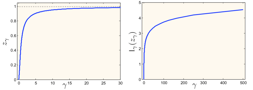
Figure 1: The plots of mappings $\gamma\mapsto z_{\gamma}$ and $\gamma\mapsto{\sf l}_{\gamma}(z_{\gamma})$.

5 Tightness of the assumptions

In this section, we assume that the errors $\varepsilon_{i}$ are i.i.d. Gaussian with zero mean and variance $1$ and we focus our attention on the functional class $\widetilde{\Sigma}(\kappa,L)$ of all functions satisfying assumption [C2($\kappa,L$)]. In order to avoid irrelevant technicalities and to better convey the main results, we assume that $\kappa=1$ and denote $\widetilde{\Sigma}_{L}=\widetilde{\Sigma}(1,L)$. Furthermore, we will assume that the design $\boldsymbol{X}_{1},\ldots,\boldsymbol{X}_{n}$ is fixed and satisfies

$$\frac{1}{n}\sum_{i=1}^{n}\varphi_{\boldsymbol{k}}(\boldsymbol{X}_{i})\varphi_{{\boldsymbol{k}}^{\prime}}(\boldsymbol{X}_{i})\leq\frac{n}{N_{1}(d^{*},L)^{2}}$$ (6)

for all distinct ${\boldsymbol{k}}$, ${{\boldsymbol{k}}^{\prime}}\in S_{(d^{*}L)^{1/2},d^{*}}\subset\mathbb Z^{d}$. The goal in this section is to provide conditions under which the consistent estimation of the sparsity support is impossible, that is there exists a positive constant $c>0$ and an integer $n_{0}\in\mathbb N$ such that, if $n\geq n_{0}$,

$$\inf_{\widetilde{J}}\sup_{{\sf f}\in\widetilde{\Sigma}_{L}}\mathbf{P}_{\sf f}(\widetilde{J}\neq J_{\sf f})\geq c,$$

where the $\inf$ is over all possible estimators of $J_{\sf f}$. To lower bound the LHS of the last inequality, we introduce a set of $M+1$ probability distributions $\mu_{0},\ldots,\mu_{M}$ on $\tilde{\Sigma}_{L}$ and use the fact that

$$\inf_{\widetilde{J}}\sup_{{\sf f}\in\widetilde{\Sigma}_{L}}\mathbf{P}_{\sf f}(\widetilde{J}\neq J_{\sf f})\geq\inf_{\widetilde{J}}\frac{1}{M+1}\sum_{\ell=0}^{M}\int_{\widetilde{\Sigma}_{L}}\mathbf{P}_{\sf f}(\widetilde{J}\neq J_{\sf f})\,\mu_{\ell}(d{\sf f}).$$ (7)

These measures $\mu_{\ell}$ will be chosen in such a way that for each $\ell\geq 1$ there is a set $J_{\ell}$ of cardinality $d^{*}$ such that $\mu_{\ell}\{J_{\sf f}=J_{\ell}\}=1$ and all the sets $J_{1},\ldots,J_{M}$ are distinct. The measure $\mu_{0}$ is the Dirac measure in $0$. Considering these $\mu_{\ell}$s as “prior” probability measures on $\tilde{\Sigma}_{L}$ and defining the corresponding “posterior” probability measures $\mathbb P_{0},\mathbb P_{1},\ldots,\mathbb P_{M}$ by

$$\mathbb P_{\ell}(A)=\int_{\tilde{\Sigma}_{L}}\mathbf{P}_{\sf f}(A)\,\mu_{\ell}(d{\sf f}),\quad\text{for every measurable set }A\subset\mathbb R^{n},$$

we can write the inequality (7) as

$$\inf_{\widetilde{J}}\sup_{{\sf f}\in\widetilde{\Sigma}_{L}}\mathbf{P}_{\sf f}(\widetilde{J}\neq J_{\sf f})\geq\inf_{\psi}\frac{1}{M+1}\sum_{\ell=0}^{M}\mathbb P_{\ell}(\psi\not=\ell),$$ (8)

where the $\inf$ is taken over all random variables $\psi$ taking values in $\{0,\ldots,M\}$. The latter $\inf$ will be controlled using a suitable version of the Fano lemma, see Fano (1961). In what follows, we denote by $\mathcal{K}(P,Q)$ the Kullback-Leibler divergence between two probability measures $P$ and $Q$ defined on the same probability space.

Lemma 1 (Corollary 2.6 of Tsybakov (2009)).

Let $(\mathcal{X},\mathcal{A})$ be a measurable space and let $P_{0},\ldots,P_{M}$ be probability measures on $(\mathcal{X},\mathcal{A})$. Let us set $\bar{p}_{e,M}=\inf_{\psi}(M+1)^{-1}\sum_{\ell=0}^{M}P_{\ell}\big{(}\psi\not=\ell\big{)}$ where the $\inf$ is taken over all measurable functions $\psi:\mathcal{X}\to\big{\{}0,\ldots,M\big{\}}$. If for some $0<\alpha<1$

$$\frac{1}{M+1}\sum_{\ell=0}^{M}\mathcal{K}\big{(}P_{\ell},P_{0}\big{)}\leq\alpha\log M,$$

then

$$\bar{p}_{e,M}\geq\frac{\log(M+1)-\log 2}{\log M}-\alpha.$$

It follows from this lemma that one can deduce a lower bound on $\bar{p}_{e,M}$, which is the quantity we are interested in, from an upper bound on the average Kullback-Leibler divergence between the measures $\mathbb P_{\ell}$ and $\mathbb P_{0}$. This roughly means that the measures $\mu_{\ell}$ should not be very far from $\mu_{0}$ but the probability measures $\mu_{\ell}$ should be very different one from another in terms of the sparsity pattern of a function ${\sf f}$ randomly drawn according to $\mu_{\ell}$. This property is ensured by the following result.

Lemma 2.

Suppose $\mu_{0}=\delta_{0}$, the Dirac measure at 0$\in\Sigma_{L}$. Let $S$ be a subset of $\mathbb Z^{d}$ of cardinality ${|S|}$ and $A$ be a constant. Define $\mu_{S}$ as a discrete measure supported on the finite set of functions $\{{\sf f}_{\boldsymbol{\omega}}=\sum_{{\boldsymbol{k}}\in S}A\omega_{\boldsymbol{k}}\varphi_{\boldsymbol{k}}:{\boldsymbol{\omega}}\in\{\pm 1\}^{S}\}$ such that $\mu_{S}({\sf f}={\sf f}_{\boldsymbol{\omega}})=2^{-{|S|}}$ for every ${\boldsymbol{\omega}}\in\{\pm 1\}^{S}$, i.e., the $\omega_{\boldsymbol{k}}$’s are i.i.d.  Rademacher random variables under $\mu_{S}$. If, for some $\epsilon\geq 0$, the condition

$$\frac{1}{n}\sum_{i=1}^{n}\varphi_{\boldsymbol{k}}(\boldsymbol{X}_{i})\varphi_{{\boldsymbol{k}}^{\prime}}(\boldsymbol{X}_{i})\leq\epsilon\qquad\forall{\boldsymbol{k}},{{\boldsymbol{k}}^{\prime}}\in S$$

is fulfilled, then

$$\mathcal{K}(\mathbb P_{1},\mathbb P_{0})\leq\log\bigg{[}\int\Big{(}\frac{d\mathbb P_{1}}{d\mathbb P_{0}}\,(\boldsymbol{y})\Big{)}^{2}\mathbb P_{0}(d\!\boldsymbol{y})\bigg{]}\leq{4|S|A^{4}n^{2}}\Big{\{}1+\frac{|S|\epsilon}{4nA^{2}}\Big{\}}.$$

These evaluations lead to the following theorem, that tells us that the conditions to which we have resorted for proving the consistency in Section 3 are nearly optimal.

Theorem 2.

Let the design $\boldsymbol{X}_{1},\ldots,\boldsymbol{X}_{n}\in[0,1]^{d}$ be deterministic and satisfy (6). Let $\gamma^{*}$ the largest real number such that $d^{*}\gamma^{*}$ is integer and $L\geq\gamma^{*}(1+{1}/{2z_{\gamma^{*}}})$. If for some positive number $\alpha<({\log 3-\log 2})/{\log 3}$

$$\frac{(N_{1}(d^{*},\gamma^{*})-N_{2}(d^{*},\gamma^{*}))^{2}\log\binom{d}{d^{*}}}{n^{2}N_{1}(d^{*},\gamma^{*})}\geq\frac{\alpha}{5},$$ (9)

then there exists a positive constant $c>0$ and a $d_{0}\in\mathbb N$ such that, if $d^{*}\geq d_{0}$,

$$\inf_{\widetilde{J}}\sup_{{\sf f}\in\widetilde{\Sigma}_{L}}\mathbf{P}_{\sf f}(\widetilde{J}\neq J_{\sf f})\geq c.$$

Proof.

We apply the Fano lemma with $M=\binom{d}{d^{*}}$. We choose $\mu_{0},\ldots,\mu_{M}$ as follows. $\mu_{0}$ is the Dirac measure $\delta_{0}$, $\mu_{1}$ is defined as in Lemma 2 with $S=\mathcal{C}_{1}(d^{*},\gamma^{*})$ and $A={\big{[}N_{1}(d^{*},\gamma^{*})-N_{2}(d^{*},\gamma^{*})\big{]}}^{-1/2}$. The measures $\mu_{2},\ldots,\mu_{M}$ are defined similarly and correspond to the $M-1$ remaining sparsity patterns of cardinality $d^{*}$.

In view of inequality (8) and Lemma 1, it suffices to show that the measures $\mu_{\ell}$ satisfy $\mu_{\ell}(\widetilde{\Sigma}_{L})=1$ and $\sum_{\ell=0}^{M}\mathcal{K}(\mathbb P_{\ell},\mathbb P_{0})\leq(M+1)\alpha\log M$. Combining Lemma 2 with $|S|=N_{1}(d^{*},\gamma^{*})$ and condition (6), one easily checks that equation (9) implies the desired bound on $\sum_{\ell=0}^{M}\mathcal{K}(\mathbb P_{\ell},\mathbb P_{0})$.

Let us show now that $\mu_{1}(\widetilde{\Sigma}_{L})=1$. By symmetry, this will imply that $\mu_{\ell}(\widetilde{\Sigma}_{L})=1$ for every $\ell$. Since $\mu_{1}$ is supported by the set $\{{\sf f}_{\boldsymbol{\omega}}:{\boldsymbol{\omega}}\in\{\pm 1\}^{\mathcal{C}(d^{*},\gamma^{*})}\}$, it is clear that

$$\sum_{k_{1}\neq 0}\theta_{\boldsymbol{k}}^{2}[{\sf f}_{\boldsymbol{\omega}}]=A^{2}[N_{1}(d^{*},\gamma^{*})-N_{2}(d^{*},\gamma^{*})]=1$$

and, for every $j=1,\ldots,d^{*}$,

$$\sum_{{\boldsymbol{k}}\in\mathbb Z^{d}}k_{j}^{2}\theta_{\boldsymbol{k}}^{2}[{\sf f}_{\boldsymbol{\omega}}]=\sum_{{\boldsymbol{k}}\in\mathcal{C}(d^{*},\gamma^{*})}k_{j}^{2}A^{2}=\frac{1}{d^{*}}\sum_{j=1}^{d^{*}}\sum_{{\boldsymbol{k}}\in\mathcal{C}(d^{*},\gamma^{*})}k_{j}^{2}A^{2}\leq A^{2}\gamma^{*}N_{1}(d^{*},\gamma^{*}).$$

By virtue of Proposition 1, as $d^{*}$ tends to infinity, ${N_{1}(d^{*},\gamma^{*})}/{N_{2}(d^{*},\gamma^{*})}$ is asymptotically equivalent to ${\sf h}(z_{\gamma^{*}})>1+2z_{\gamma^{*}}$. Hence, for $d^{*}$ large enough,

$$A^{2}N_{1}(d^{*},\gamma^{*})=\frac{N_{1}(d^{*},\gamma^{*})}{N_{1}(d^{*},\gamma^{*})-N_{2}(d^{*},\gamma^{*})}<\frac{1}{2z_{\gamma^{*}}}+1.$$

As a consequence, for every $j=1,\ldots,d^{*}$,

$$\sum_{{\boldsymbol{k}}\in\mathbb Z^{d}}k_{j}^{2}\theta_{\boldsymbol{k}}^{2}[{\sf f}_{\boldsymbol{\omega}}]\leq\gamma^{*}\Big{(}\frac{1}{2z_{\gamma^{*}}}+1\Big{)}\leq L,$$

where the last inequality follows from the definition of $\gamma^{*}$. ∎

Note that Theorem 2 is concerned by the case where the intrinsic dimension is not too small, which is the most interesting case in the present context. However, a much simpler result can be established showing that the conditions of Theorem 1 are tight in the case of fixed intrinsic dimension as well.

Proposition 2.

Let the design $\boldsymbol{X}_{1},\ldots,\boldsymbol{X}_{n}\in[0,1]^{d}$ be either deterministic or random. If for some positive $\alpha<{(\log 3-\log 2)}/{\log 3}$, the inequality

$$\frac{d^{*}\big{(}\log d-\log d^{*}\big{)}}{n}\geq\alpha^{-1}$$

holds true, then there is a constant $c>0$ such that $\inf_{\widetilde{J}_{n}}\sup_{f\in\widetilde{\Sigma}_{L}}\mathbf{P}_{\sf f}(\widetilde{J}_{n}\neq J_{\sf f})\geq c$.

6 Discussion

The results proved in previous sections almost exhaustively answer the questions on the existence of consistent estimators of the sparsity pattern in the problem of nonparametric regression. In fact as far as only rates of convergence are of interest, the result obtained in Theorem 1 is shown in Section 5 to be unimprovable. Thus only the problem of finding sharp constants remains open. To make these statements more precise, let us consider the simplified set-up $\sigma=\kappa=1$ and define the following two regimes:

1. The regime of fixed sparsity, i.e., when the sample size $n$ and the ambient dimension $d$ tend to infinity but the intrinsic dimension $d^{*}$ remains constant or bounded.

2. The regime of increasing sparsity, i.e., when the intrinsic dimension $d^{*}$ tends to infinity along with the sample size $n$ and the ambient dimension $d$. For simplicity, we will assume that $d^{*}=O(d^{1-\epsilon})$ for some $\epsilon>0$.

In the fixed sparsity regime, in view of Theorem 1, consistent estimation of the sparsity pattern can be achieved using the estimator $\widehat{J}$ as soon as $(\log d)/n\leq c_{\star}$, where $c_{\star}$ is the constant defined by

$$c_{\star}=\min\Big{(}\frac{L_{2}^{2}}{2d^{*}L_{\infty}^{2}},\frac{g_{\min}^{2}}{2^{8}(1+L_{2})^{2}d^{*}N(d^{*},2L)}\Big{)}.$$

This follows from the fact that the tuning parameter $m$ is fixed and that the probability of the error, bounded by $3(6md)^{d^{*}}$ tends to zero as $d\to\infty$. On the other hand, by virtue of Proposition 2, consistent estimation of the sparsity pattern is impossible if $(\log d)/n>c^{\star}$, where $c^{\star}=2\log 3/(d^{*}\log(3/2))$. Thus, up to multiplicative constants $c_{\star}$ and $c^{\star}$ (which are clearly not sharp), the result of Theorem 1 can not be improved.

In the regime of increasing sparsity, the second inequality in (4) is the most stringent one. Taking the logarithm of both sides and using formula (5) for $N(d^{*},2L)=N_{1}(d^{*},2L)-N_{2}(d^{*},2L)$, we see that consistent estimation of $J$ is possible when

$$\underline{c}_{1}d^{*}+\frac{1}{2}\log d^{*}+\log\log d-\log n<\underline{c}_{2},$$ (10)

with $\underline{c}_{1}={\sf l}_{2L}(z_{2L})$ and $\underline{c}_{2}=2(\log(g_{\min})-\log(17(\sigma+L_{2}))+\log\Big{\{}\frac{{\sf h}(z_{2L})z_{2L}(1-z_{2L})(2{\sf l}_{2L}^{\prime\prime}(z_{2L})\pi)^{1/2}}{{\sf h}(z_{2L})-1}\Big{\}}$. On the other hand, by virtue of (5), $\log\Big{\{}\frac{[N_{1}(d^{*},\gamma)-N_{2}(d^{*},\gamma)]^{2}}{N_{1}(d^{*},\gamma)}\Big{\}}=d^{*}{\sf l}_{\gamma}(z_{\gamma})-\frac{1}{2}\log d^{*}-\log\Big{\{}\frac{{\sf h}(z_{\gamma})^{2}z_{\gamma}(1-z_{\gamma})(2{\sf l}_{\gamma}^{\prime\prime}(z_{\gamma})\pi)^{1/2}}{({\sf h}(z_{\gamma})-1)^{2}}\Big{\}}+o(1)$. Therefore, Theorem 2 yields that it is impossible to consistently estimate $J$ if

$$\bar{c}_{1}d^{*}+\frac{1}{2}\log d^{*}+\log\log d-2\log n>\bar{c}_{2},$$ (11)

where $\bar{c}_{1}={\sf l}_{\gamma^{*}}(z_{\gamma^{*}})$ and $\bar{c}_{2}=\log\Big{\{}\frac{{\sf h}(z_{\gamma^{*}})^{2}z_{\gamma^{*}}(1-z_{\gamma^{*}})(2{\sf l}_{\gamma^{*}}^{\prime\prime}(z_{\gamma^{*}})\pi)^{1/2}}{({\sf h}(z_{\gamma^{*}})-1)^{2}}\Big{\}}+\log\log(3/2)-\log 5-\log\log 3$. A very simple consequence of inequalities (10) and (11) is that the consistent recovery of the sparsity pattern is possible under the condition $d^{*}/\log n\to 0$ and impossible for $d^{*}/\log n\to\infty$ as $n\to\infty$, provided that $\log\log d=o(\log n)$.

Let us stress now that, all over this work, we have deliberately avoided any discussion on the computational aspects of the variable selection in nonparametric regression. The goal in this paper was to investigate the possibility of consistent recovery without paying attention to the complexity of the selection procedure. This lead to some conditions that could be considered a benchmark for assessing the properties of sparsity pattern estimators. As for the estimator proposed in Section 3, it is worth noting that its computational complexity is not always prohibitively large. A recommended strategy is to compute the coefficients $\widehat{\hskip 0.4pt\theta}_{\boldsymbol{k}}$ in a stepwise manner; at each step $K=1,2,\ldots,d^{*}$ only the coefficients $\widehat{\hskip 0.4pt\theta}_{\boldsymbol{k}}$ with $\|{\boldsymbol{k}}\|_{0}=K$ need to be computed and compared with the threshold. If some $\widehat{\hskip 0.4pt\theta}_{\boldsymbol{k}}$ exceeds the threshold, then all the covariates $X^{j}$ corresponding to nonzero coordinates of ${\boldsymbol{k}}$ are considered as relevant. We can stop this computation as soon as the number of covariates classified as relevant attains $d^{*}$. While the worst-case complexity of this procedure is exponential, there are many functions ${\sf f}$ for which the complexity of the procedure will be polynomial in $d$. For example, this is the case for additive models in which ${\sf f}(\boldsymbol{x})={\sf f}_{1}(x_{i_{1}})+\ldots+{\sf f}_{d^{*}}(x_{i_{d^{*}}})$ for some univariate functions ${\sf f}_{1},\ldots,{\sf f}_{d^{*}}$.

Appendix A Proof of Theorem 1

The empirical Fourier coefficients can be decomposed as follows:

$$\widehat{\hskip 0.4pt\theta}_{\boldsymbol{k}}=\tilde{\theta}_{\boldsymbol{k}}+z_{\boldsymbol{k}},\qquad\text{where}\qquad\tilde{\theta}_{\boldsymbol{k}}=\frac{1}{n}\sum_{i=1}^{n}\frac{\varphi_{\boldsymbol{k}}(\boldsymbol{X}_{i})}{{\sf g}(\boldsymbol{X}_{i})}{\sf f}(\boldsymbol{X}_{i})\qquad\text{and}\qquad z_{\boldsymbol{k}}=\frac{\sigma}{n}\sum_{i=1}^{n}\frac{\varphi_{\boldsymbol{k}}(\boldsymbol{X}_{i})}{{\sf g}(\boldsymbol{X}_{i})}\varepsilon_{i}.$$ (12)

If, for a multi index ${\boldsymbol{k}}$, $\theta_{\boldsymbol{k}}=0$, then the corresponding empirical Fourier coefficient will be close to zero with high probability. To show this, let us first look at what happens with $z_{\boldsymbol{k}}$’s. We have, for every real number $x$,

$$\mathbf{P}\big{(}|z_{\boldsymbol{k}}|>x\,\big{|}\,\boldsymbol{X}_{1},\ldots,\boldsymbol{X}_{n}\big{)}\leq\exp\Big{(}-\frac{x^{2}}{2\sigma_{\boldsymbol{k}}^{2}}\Big{)}\quad\forall{\boldsymbol{k}}\in S_{m,d^{*}}$$

with

$$\sigma_{\boldsymbol{k}}^{2}=\frac{\sigma^{2}}{n^{2}}\sum_{i=1}^{n}\frac{\varphi_{\boldsymbol{k}}(\boldsymbol{X}_{i})^{2}}{{\sf g}(\boldsymbol{X}_{i})^{2}}\leq\frac{2\sigma^{2}}{g_{\min}^{2}n}.$$

Therefore, for every ${\boldsymbol{k}}\in S_{m,d^{*}}$, it holds that $\mathbf{P}\big{(}|z_{\boldsymbol{k}}|>x|\boldsymbol{X}_{1},\ldots,\boldsymbol{X}_{n}\big{)}\leq\exp({-ng_{\min}^{2}x^{2}}/{4\sigma^{2}})$. This entails that by setting $\lambda_{1}=({8\sigma^{2}d^{*}\log(6md)}/{ng_{\min}^{2}})^{1/2}$ and by using the inequalities

$$\text{Card}(S_{m,d^{*}}) =\sum_{i=0}^{d^{*}}\binom{d}{i}(2m)^{i}\leq(2m)^{d^{*}}\sum_{i=0}^{d^{*}}\frac{d^{i}}{i!}$$

$$\leq 3(2md)^{d^{*}}\leq(6md)^{d^{*}},$$

we get

$$\mathbf{P}\Big{(}\max_{{\boldsymbol{k}}\in S_{m,d^{*}}}|z_{\boldsymbol{k}}|>\lambda_{1}\,|\,\boldsymbol{X}_{1},\ldots,\boldsymbol{X}_{n}\Big{)} \leq\sum_{{\boldsymbol{k}}\in S_{m,d^{*}}}\mathbf{P}\Big{(}|z_{\boldsymbol{k}}|>\lambda_{1}\,|\,\boldsymbol{X}_{1},\ldots,\boldsymbol{X}_{n}\Big{)}$$

$$\leq\text{Card}(S_{m,d^{*}})e^{-ng_{\min}^{2}\lambda_{1}^{2}/{4\sigma^{2}}}\leq(6md)^{-d^{*}}.$$

Next, we use a concentration inequality for controlling large deviations of $\tilde{\theta}_{\boldsymbol{k}}$’s from $\theta_{\boldsymbol{k}}$’s. Recall that in view of the definition $\tilde{\theta}_{\boldsymbol{k}}=\frac{1}{n}\sum_{i=1}^{n}\frac{\varphi_{\boldsymbol{k}}(\boldsymbol{X}_{i})}{{\sf g}(\boldsymbol{X}_{i})}{\sf f}(\boldsymbol{X}_{i})$, we have $\mathbb E(\tilde{\theta}_{\boldsymbol{k}})=\theta_{\boldsymbol{k}}$. By virtue of the boundedness of ${\sf f}$, it holds that $|\frac{\varphi_{\boldsymbol{k}}(\boldsymbol{X}_{i})}{{\sf g}(\boldsymbol{X}_{i})}{\sf f}(\boldsymbol{X}_{i})|\leq{\sqrt{2}L_{\infty}}/{g_{\min}}$. Furthermore, the bound $V\triangleq\text{Var}\big{(}\frac{\varphi_{\boldsymbol{k}}(\boldsymbol{X}_{i})}{{\sf g}(\boldsymbol{X}_{i})}{\sf f}(\boldsymbol{X}_{i})\big{)}\leq\int f^{2}(\boldsymbol{x})\frac{\varphi_{\boldsymbol{k}}^{2}(\boldsymbol{x})}{{\sf g}(\boldsymbol{x})}d\boldsymbol{x}\leq{2L_{2}^{2}}/{g_{\min}^{2}}$ combined with Bernstein’s inequality yields

$$\mathbf{P}\big{(}|\tilde{\theta}_{\boldsymbol{k}}-\theta_{\boldsymbol{k}}|>t\big{)} \leq 2\exp\Big{(}-\frac{nt^{2}}{2(V+{t\sqrt{2}L_{\infty}/3g_{\min}})}\Big{)}$$

$$\leq 2\exp\Big{(}-\frac{g_{\min}^{2}nt^{2}}{4L_{2}^{2}+{tL_{\infty}}g_{\min}}\Big{)},\qquad\forall t>0.$$

Let us define $\lambda_{2}=4L_{2}\Big{(}{\frac{d^{*}\log(6md)}{ng_{\min}^{2}}}\Big{)}^{1/2}$. Then,

$$\mathbf{P}\big{(}|\tilde{\theta}_{\boldsymbol{k}}-\theta_{\boldsymbol{k}}|>\lambda_{2}\big{)}\leq 2\exp\bigg{(}-\frac{4L_{2}^{2}d^{*}\log(6md)}{L_{2}^{2}+L_{\infty}L_{2}\big{(}{\frac{d^{*}\log(6md)}{n}}\big{)}^{1/2}}\bigg{)}.$$

The first inequality in condition (4) implies that the denominator in the exponential is not larger than $2L_{2}^{2}$. Hence,

$$\mathbf{P}\Big{(}\max_{{\boldsymbol{k}}\in S_{m,d^{*}}}|\tilde{\theta}_{\boldsymbol{k}}-\theta_{\boldsymbol{k}}|>\lambda_{2}\Big{)}\leq 2/{(6md)^{d^{*}}}.$$

Let $\mathcal{A}_{1}=\big{\{}\max_{{\boldsymbol{k}}\in S_{m,d^{*}}}|z_{\boldsymbol{k}}|\leq\lambda_{1}\big{\}}$ and $\mathcal{A}_{2}=\big{\{}\max_{{\boldsymbol{k}}\in S_{m,d^{*}}}|\tilde{\theta}_{\boldsymbol{k}}|\leq\lambda_{2}\big{\}}$. One easily checks that

$$\mathbf{P}\big{(}J^{c}\not\subset\widehat{J}^{c}\big{)}\leq\mathbf{P}\big{(}\mathcal{A}_{1}^{c}\big{)}+\mathbf{P}\big{(}\mathcal{A}_{2}^{c}\big{)}\leq 3/(6md)^{d^{*}}.$$

As for the converse inclusion, we have

$$\mathbf{P}(J\not\subset\widehat{J}) \leq\mathbf{P}\Big{(}\exists j\in J\ \text{s.t.}\ \max_{{\boldsymbol{k}}\in S_{m,d^{*}}:\,k_{j}\not=0}|\widehat{\hskip 0.4pt\theta}_{\boldsymbol{k}}|\leq{\lambda}\Big{)}$$

$$\leq\mathbf{1}\Big{\{}\exists j\in J\ \text{s.t.}\ \max_{{\boldsymbol{k}}\in S_{m,d^{*}}\,:k_{j}\not=0}|\theta_{\boldsymbol{k}}|\leq 2\lambda\Big{\}}+\mathbf{P}\big{(}\mathcal{A}_{1}^{c}\big{)}+\mathbf{P}\big{(}\mathcal{A}_{2}^{c}\big{)}.$$

We show now that the first term in the last line is equal to zero. If this was not the case, then for some value $j_{0}$ we would have $Q_{j_{0}}\geq\kappa$ and $|\theta_{\boldsymbol{k}}|\leq 2\lambda$, for all ${\boldsymbol{k}}\in S_{m,d^{*}}$ such that $k_{j_{0}}\not=0$. This would imply that

$$Q_{j_{0},m,d^{*}}{\triangleq}\sum_{{\boldsymbol{k}}\in S_{m,d^{*}}\,:k_{j_{0}}\not=0}\theta_{\boldsymbol{k}}^{2}\leq 4\lambda^{2}N(d^{*},^{2}L/\kappa).$$

On the other hand,

$$Q_{j_{0}}-Q_{j_{0},m,d^{*}} \leq\sum_{\|{\boldsymbol{k}}\|_{2}\geq m}\theta_{\boldsymbol{k}}^{2}\leq m^{-2}\sum_{\|{\boldsymbol{k}}\|_{2}\geq m}\sum_{j\in J}k_{j}^{2}\theta_{\boldsymbol{k}}^{2}\leq\frac{Ld^{*}}{m^{2}}.$$

Remark now that the choice of the truncation parameter $m$ proposed in the statement of the proposition implies that $Q_{j_{0}}-Q_{j_{0},m,d^{*}}\leq\kappa/2$. Combining these estimates, we get $Q_{j_{0}}\leq\frac{\kappa}{2}+4\lambda^{2}N(d^{*},m^{2}/d^{*}),$ which is impossible since $Q_{j_{0}}\geq\kappa$.

Appendix B Proof of Proposition 1

Proof of the first assertion.

This proof can be found in Mazo and Odlyzko (1990), we repeat here the arguments therein for the sake of keeping the paper self-contained. Recall that $N_{1}(d^{*},\gamma)$ admits an integral representation with the integrand:

$$\frac{{\sf h}(z)^{d^{*}}}{z^{\gamma d^{*}}}\frac{1}{z(1-z)}=\frac{1}{z(1-z)}\exp\bigg{[}d^{*}\log\bigg{(}\frac{{\sf h}(z)}{z^{\gamma}}\bigg{)}\bigg{]}.$$

For any real number $y>0$, we define $\phi(y)=e^{-y}{\sf h}^{\prime}(e^{-y})/{\sf h}(e^{-y})=\sum_{k=-\infty}^{k=+\infty}k^{2}e^{-yk^{2}}/\sum_{k=-\infty}^{k=+\infty}e^{-yk^{2}}$ in such a way that

$$\phi(y)=\gamma\quad\Longleftrightarrow\quad\frac{{\sf h}^{\prime}(e^{-y})}{{\sf h}(e^{-y})}=\frac{\gamma}{e^{-y}}\quad\Longleftrightarrow\quad{\sf l}_{\gamma}^{\prime}(e^{-y})=0.$$

By virtue of the Cauchy-Schwarz inequality, it holds that

$$\sum k^{4}e^{-yk^{2}}\sum e^{-yk^{2}}>\Big{(}\sum k^{2}e^{-yk^{2}}\Big{)}^{2},\quad\forall y\in(0,\infty),$$

implying that $\phi^{\prime}(y)<0$ for all $y\in(0,\infty)$, i.e., $\phi$ is strictly decreasing. Furthermore, $\phi$ is obviously continuous with $\lim_{y\to 0}\phi(y)=+\infty$ and $\lim_{y\to\infty}\phi(y)=0$. These properties imply the existence and the uniqueness of $y_{\gamma}\in(0,\infty)$ such that ${\phi(y_{\gamma})}=\gamma$. Furthermore, as the inverse of a decreasing function, the function $\gamma\mapsto y_{\gamma}$ is decreasing as well. We set $z_{\gamma}=e^{-y_{\gamma}}$ so that $\gamma\mapsto z_{\gamma}$ is increasing.

We also have

$${\sf l}_{\gamma}^{\prime\prime}(z_{\gamma}) =\frac{{\sf h}^{\prime\prime}{\sf h}-({\sf h}^{\prime})^{2}}{{\sf h}^{2}}(z_{\gamma})+\frac{\gamma}{z_{\gamma}^{2}}=z_{\gamma}^{-2}\bigg{\{}\frac{\sum_{k}(k^{4}-k^{2})z_{\gamma}^{k^{2}}}{\sum_{k}z_{\gamma}^{k^{2}}}-\bigg{(}\frac{\sum_{k}k^{2}z_{\gamma}^{k^{2}}}{\sum_{k}z_{\gamma}^{k^{2}}}\bigg{)}^{2}+\gamma\bigg{\}}$$

$$=z_{\gamma}^{-2}\big{\{}-\phi^{\prime}(y_{\gamma})-\phi(y_{\gamma})+\gamma\big{\}}=-z_{\gamma}^{-2}\phi^{\prime}(y_{\gamma})>0.$$

Proof of the second assertion.

We apply the saddle-point method to the integral representing $N_{1}$ see, e.g., Chapter IX in Dieudonné (1968). It holds that

$$N_{1}(d^{*},\gamma)=\frac{1}{2\pi i}\oint_{|z|=z_{\gamma}}\frac{{\sf h}(z)^{d^{*}}}{z^{\gamma d^{*}}}\frac{dz}{z(1-z)}=\frac{1}{2\pi i}\oint_{|z|=z_{\gamma}}\{z(1-z)\}^{-1}e^{d^{*}{\sf l}_{\gamma}(z)}{dz}.$$ (13)

The first assertion of the proposition provided us with a real number $z_{\gamma}$ such that ${\sf l}_{\gamma}^{\prime}(z_{\gamma})=0$ et ${\sf l}_{\gamma}^{\prime\prime}(z_{\gamma})>0$. The tangent to the steepest descent curve at $z_{\gamma}$ is vertical. The path we choose for integration is the circle with center 0 and radius $z_{\gamma}$. As this circle and the steepest descent curve have the same tangent at $z_{\gamma}$, applying formula (1.8.1) of Dieudonné (1968) (with $\alpha=0$ since ${\sf l}^{\prime\prime}(z_{\gamma})$ is real and positive), we get that

$$\frac{1}{2\pi i}\oint_{|z|=z_{\gamma}}\{z(1-z)\}^{-1}e^{d^{*}{\sf l}_{\gamma}(z)}{dz}=\frac{1}{2\pi i}\sqrt{\frac{2\pi}{d^{*}{\sf l}_{\gamma}^{\prime\prime}(z_{\gamma})}}e^{{\rm i\pi/2}}\{z_{\gamma}(1-z_{\gamma})\}^{-1}e^{d^{*}{\sf l}_{\gamma}(z_{\gamma})}(1+o(1)),$$

when $d^{*}\to\infty$, as soon as the condition $\Re[{\sf l}_{\gamma}(z)-{\sf l}_{\gamma}(z_{\gamma})]\leq-\mu$ is satisfied for some $\mu>0$ and for any $z$ belonging to the circle $|z|=|z_{\gamma}|$ and lying not too close to $z_{\gamma}$. To check that this is indeed the case, we remark that $\Re[{\sf l}_{\gamma}(z)]=\log\big{|}\frac{{\sf h}(z)}{z^{\gamma}}\big{|}$. Hence, if $z=z_{\gamma}e^{{\rm i}\omega}$ with $\omega\in[\omega_{0},2\pi-\omega_{0}]$ for some $\omega_{0}\in]0,\pi[$, then

$$\Big{|}\frac{{\sf h}(z)}{z^{\gamma}}\Big{|}=\frac{|1+2z+2\sum_{k>1}z^{k^{2}}|}{z_{\gamma}^{\gamma}}\leq\frac{|1+z|+z_{\gamma}+2\sum_{k>1}z_{\gamma}^{k^{2}}}{z_{\gamma}^{\gamma}}\leq\frac{|1+e^{{\rm i}\omega_{0}}z_{\gamma}|+z_{\gamma}+2\sum_{k>1}z_{\gamma}^{k^{2}}}{z_{\gamma}^{\gamma}}.$$

Therefore $\Re[{\sf l}_{\gamma}(z)-\Re{\sf l}_{\gamma}(z_{\gamma})]\leq-\mu$ with $\mu=\log\Big{(}\frac{1+2z_{\gamma}+\sum_{k\geq 1}z_{\gamma}^{k^{2}}}{|1+z_{\gamma}e^{{\rm i}\omega_{0}}|+z_{\gamma}+\sum_{k\geq 1}z_{\gamma}^{k^{2}}}\Big{)}>0$. This completes the proof for the term $N_{1}(d^{*},\gamma)$. The term $N_{2}(d^{*},\gamma)$ can be dealt in the same way.

Appendix C Proof of Lemma 2

Let $\phi(\cdot)$ be the density of $\mathcal{N}(0,1)$ and let

$$p_{\sf f}(\boldsymbol{y})\triangleq\prod_{i=1}^{n}\phi\Big{(}y_{i}-{\sf f}(\boldsymbol{X}_{i})\Big{)},\qquad\forall\boldsymbol{y}\in\mathbb R^{n}.$$

Since the errors $\varepsilon_{i}$ are Gaussian, the posterior probabilities $\mathbb P_{0}$ and $\mathbb P_{1}$ are absolutely continuous w.r.t. the Lebesgue measure on $\mathbb R^{n}$ and admit the densities

$$p_{0}(\boldsymbol{y})=\prod_{i=1}^{n}\phi(y_{i}),\qquad\text{and}\qquad p_{1}(\boldsymbol{y})=\mathbf{E}_{{\sf f}\sim\mu_{S}}p_{\sf f}(\boldsymbol{y}),\qquad\forall\boldsymbol{y}\in\mathbb R^{n}.$$

Simple algebra yields:

$$p_{\sf f}(\boldsymbol{y})=C_{\sf f}p_{0}(\boldsymbol{y})\prod_{i=1}^{n}\exp\Big{\{}y_{i}{\sf f}(\boldsymbol{X}_{i})\Big{\}},\quad\forall\boldsymbol{y}\in\mathbb R^{n},$$

where $C_{\sf f}=\prod_{i=1}^{n}\exp\big{\{}-{\sf f}(\boldsymbol{X}_{i})^{2}/2\big{\}}$. Thus,

$$\frac{p_{1}}{p_{0}}(\boldsymbol{y})=\mathbf{E}_{{\sf f}\sim\mu_{S}}\Big{[}C_{\sf f}\prod_{i=1}^{n}\exp\Big{\{}{y_{i}}{\sf f}(\boldsymbol{X}_{i})\Big{\}}\Big{]}.$$

Therefore,

$$\int_{\mathbb R^{n}}\Big{(}\frac{p_{1}}{p_{0}}(\boldsymbol{y})\Big{)}^{2}p_{0}(\boldsymbol{y})d\boldsymbol{y} =\mathbf{E}_{({\sf f},{\sf f}^{\prime})\sim\mu_{S}\otimes\mu_{S}}\Big{[}C_{\sf f}C_{{\sf f}^{\prime}}\int_{\mathbb R^{n}}\prod_{i=1}^{n}\bigg{(}\exp\Big{\{}{y_{i}}({\sf f}+{\sf f}^{\prime})(\boldsymbol{X}_{i})\Big{\}}\phi(y_{i})\bigg{)}d\boldsymbol{y}\Big{]}$$

$$=\mathbf{E}_{({\sf f},{\sf f}^{\prime})\sim\mu_{S}\otimes\mu_{S}}\Big{[}C_{\sf f}C_{{\sf f}^{\prime}}\prod_{i=1}^{n}\exp\Big{(}\frac{1}{2}({\sf f}+{\sf f}^{\prime})^{2}(\boldsymbol{X}_{i})\Big{)}\Big{]}$$

$$=\mathbf{E}_{({\sf f},{\sf f}^{\prime})\sim\mu_{S}\otimes\mu_{S}}\Big{[}\exp\Big{(}\sum_{i=1}^{n}{\sf f}(\boldsymbol{X}_{i}){\sf f}^{\prime}(\boldsymbol{X}_{i})\Big{)}\Big{]}$$

$$=\frac{1}{2^{2|S|}}\sum_{{\boldsymbol{\omega}},{\boldsymbol{\omega}}^{\prime}\in\{\pm 1\}^{S}}\prod_{{\boldsymbol{k}},{{\boldsymbol{k}}^{\prime}}\in S}\exp\Big{(}\omega_{\boldsymbol{k}}\omega_{{\boldsymbol{k}}^{\prime}}^{\prime}b_{{\boldsymbol{k}}{{\boldsymbol{k}}^{\prime}}}\Big{)},$$

where $b_{{\boldsymbol{k}}{{\boldsymbol{k}}^{\prime}}}={A^{2}}\sum_{i=1}^{n}\varphi_{\boldsymbol{k}}(\boldsymbol{X}_{i})\varphi_{{\boldsymbol{k}}^{\prime}}(\boldsymbol{X}_{i})$, for all ${\boldsymbol{k}},{{\boldsymbol{k}}^{\prime}}\in S$. Note that $0\leq b_{{\boldsymbol{k}}{\boldsymbol{k}}}\leq{2A^{2}n}$ and $|b_{{\boldsymbol{k}}{{\boldsymbol{k}}^{\prime}}}|\leq{A^{2}n\epsilon}$, for all ${\boldsymbol{k}},{\boldsymbol{k}}^{\prime}\in S$ such that ${\boldsymbol{k}}^{\prime}\not={\boldsymbol{k}}$. Now, on the one hand, for a fixed pair $({\boldsymbol{\omega}},{\boldsymbol{\omega}}^{\prime})$, we have

$$\prod_{{\boldsymbol{k}}\neq{{\boldsymbol{k}}^{\prime}}}\exp\Big{(}\omega_{\boldsymbol{k}}\omega_{{\boldsymbol{k}}^{\prime}}^{\prime}b_{{\boldsymbol{k}}{{\boldsymbol{k}}^{\prime}}}\Big{)}\leq\exp\big{(}{|S|}^{2}A^{2}n\epsilon\big{)}.$$

On the other hand, if we are given a sequence of numbers $(b_{{\boldsymbol{k}}{\boldsymbol{k}}})$ indexed by $S$, we have

$$\frac{1}{2^{2|S|}}\sum_{{\boldsymbol{\omega}},{\boldsymbol{\omega}}^{\prime}}\prod_{{\boldsymbol{k}}\in S}e^{\omega_{\boldsymbol{k}}\omega_{\boldsymbol{k}}^{\prime}b_{{\boldsymbol{k}}{\boldsymbol{k}}}}=\prod_{{\boldsymbol{k}}\in S}\frac{e^{b_{{\boldsymbol{k}}{\boldsymbol{k}}}}+e^{-b_{{\boldsymbol{k}}{\boldsymbol{k}}}}}{2}\leq\prod_{{\boldsymbol{k}}\in S}e^{b_{{\boldsymbol{k}}{\boldsymbol{k}}}^{2}}\leq\exp\Big{(}{4|S|A^{4}n^{2}}\Big{)}.$$

From these remarks it results that

$$\int_{\mathbb}R^{d}\Big{(}\frac{p_{1}}{p_{0}}\;(\boldsymbol{y})\Big{)}^{2}p_{0}(\boldsymbol{y})d\!\boldsymbol{y}\leq\exp\Big{(}{4|S|A^{4}n^{2}}\Big{\{}1+\frac{|S|\epsilon}{4nA^{2}}\Big{\}}\Big{)},$$

and the claim of the lemma follows.

Appendix D Proof of Proposition 2

Let $M=\binom{d}{d^{*}}$ and let $\{{\sf f}_{0},{\sf f}_{1},\ldots,{\sf f}_{M}\}$ be a set included in $\widetilde{\Sigma}_{L}$. Let $I_{1},\ldots,I_{M}$ be all the subsets of $\{1,\ldots,d\}$ containing exactly $d^{*}$ elements somehow enumerated. Let us set ${\sf f}_{0}\equiv 0$ and define ${\sf f}_{\ell}$, for $\ell\neq 0$, by its Fourier coefficients $\{\theta^{\ell}_{\boldsymbol{k}}:{\boldsymbol{k}}\in\mathbb Z^{d}\}$ as follows:

$$\theta^{\ell}_{{\boldsymbol{k}}}=\begin{cases}1,&{\boldsymbol{k}}=(k_{1},\ldots,k_{d})=(\mathbf{1}_{1\in I_{\ell}},\ldots,\mathbf{1}_{d\in I_{\ell}}),\\ 0,&\text{otherwise}.\end{cases}$$

Obviously, all the functions ${\sf f}_{\ell}$ belong to $\Sigma$ and, moreover, each ${\sf f}_{\ell}$ has $I_{\ell}$ as sparsity pattern. One easily checks that our choice of ${\sf f}_{\ell}$ implies $\mathcal{K}(\mathbf{P}_{{\sf f}_{\ell}},\mathbf{P}_{{\sf f}_{0}})=n\|{\sf f}_{\ell}-{\sf f}_{0}\|_{2}^{2}=n$. Therefore, if $\alpha\log M=\alpha\log\binom{d}{d^{*}}\geq n$, the desired inequality is satisfied. To conclude it suffices to note that $\log\binom{d}{d^{*}}$ is larger than or equal to $d^{*}\log(d/d^{*})=d^{*}\big{(}\log d-\log d^{*}\big{)}$.

References

• Akaike (1973) Hirotsugu Akaike. Information theory and an extension of the maximum likelihood principle. In Second International Symposium on Information Theory (Tsahkadsor, 1971), pages 267–281. Akadémiai Kiadó, Budapest, 1973.
• Alquier (2008) Pierre Alquier. Iterative feature selection in least square regression estimation. Ann. Inst. Henri Poincaré Probab. Stat., 44(1):47–88, 2008.
• Bach (2009) Francis Bach. High-dimensional non-linear variable selection through hierarchical kernel learning. Technical report, arXiv:0909.0844, 2009.
• Bertin and Lecué (2008) Karine Bertin and Guillaume Lecué. Selection of variables and dimension reduction in high-dimensional non-parametric regression. Electron. J. Stat., 2:1224–1241, 2008.
• Bickel et al. (2010) Peter J. Bickel, Ya’acov Ritov, and Alexandre B. Tsybakov. Hierarchical selection of variables in sparse high-dimensional regression. Borrowing Strength: Theory Powering Applications - A Festschrift for Lawrence D. Brown. IMS Collections, 6:56–69, 2010.
• Bunea and Barbu (2009) Florentina Bunea and Adrian Barbu. Dimension reduction and variable selection in case control studies via regularized likelihood optimization. Electron. J. Stat., 3:1257–1287, 2009.
• Dieudonné (1968) Jean Dieudonné. Calcul infinitésimal. Hermann, Paris, 1968.
• Donoho and Jin (2009) David Donoho and Jiashun Jin. Feature selection by higher criticism thresholding achieves the optimal phase diagram. Philos. Trans. R. Soc. Lond. Ser. A Math. Phys. Eng. Sci., 367(1906):4449–4470, 2009. With electronic supplementary materials available online.
• Fan et al. (2009) Jianqing Fan, Richard Samworth, and Yichao Wu. Ultrahigh dimensional feature selection: beyond the linear model. J. Mach. Learn. Res., 10:2013–2038, 2009.
• Fano (1961) Robert M. Fano. Transmission of information: A statistical theory of communications. The M.I.T. Press, Cambridge, Mass., 1961.
• Jenatton et al. (2009) Rodolphe Jenatton, Jean-Yves Audibert, and Francis Bach. Structured variable selection with sparsity-inducing norms. Technical report, arXiv:0904.3523, 2009.
• Lafferty and Wasserman (2008) John Lafferty and Larry Wasserman. Rodeo: sparse, greedy nonparametric regression. Ann. Statist., 36(1):28–63, 2008.
• Laurent and Massart (2000) Beatrice Laurent and Pascal Massart. Adaptive estimation of a quadratic functional by model selection. Ann. Statist., 28(5):1302–1338, 2000.
• Lounici et al. (2010) Karim Lounici, Massimiliano Pontil, Alexandre B. Tsybakov, and Sara van de Geer. Oracle inequalities and optimal inference under group sparsity. Technical report, arXiv:1007.1771, 2010.
• Mallows (1973) Colin L. Mallows. Some comments on $C_{p}$. Technometrics, 15:661–675, Nov. 1973.
• Mazo and Odlyzko (1990) James Mazo and Andrew Odlyzko. Lattice points in high-dimensional spheres. Monatsh. Math., 110(1):47–61, 1990.
• Meinshausen and B hlmann (2010) Nicolai Meinshausen and Peter B hlmann. Stability selection. Journal Of The Royal Statistical Society Series B, 72(4):417–473, 2010.
• Obozinski et al. (2011) Guillaume Obozinski, Martin J. Wainwright, and Michael I. Jordan. High-dimensional union support recovery in multivariate. The Annals of Statistics, to appear, 2011.
• Ravikumar et al. (2010) Pradeep Ravikumar, Martin J. Wainwright, and John D. Lafferty. High-dimensional Ising model selection using $\ell_{1}$-regularized logistic regression. Ann. Statist., 38(3):1287–1319, 2010.
• Schwarz (1978) Gideon Schwarz. Estimating the dimension of a model. Ann. Statist., 6(2):461–464, 1978.
• Scott and Berger (2010) James G. Scott and James O. Berger. Bayes and empirical-Bayes multiplicity adjustment in the variable-selection problem. Ann. Statist., 38(5):2587–2619, 2010.
• Tibshirani (1996) Robert Tibshirani. Regression shrinkage and selection via the lasso. J. Roy. Statist. Soc. Ser. B, 58(1):267–288, 1996.
• Ting et al. (2010) Jo-Anne Ting, Aaron D’Souza, Sethu Vijayakumar, and Stefan Schaal. Efficient learning and feature selection in high-dimensional regression. Neural Comput., 22(4):831–886, 2010.
• Tsybakov (2009) Alexandre B. Tsybakov. Introduction to nonparametric estimation. Springer Series in Statistics. Springer, New York, 2009.
• Wasserman and Roeder (2009) Larry Wasserman and Kathryn Roeder. High-dimensional variable selection. Ann. Statist., 37(5A):2178–2201, 2009.
• Zhang (2010) Cun-Hui Zhang. Nearly unbiased variable selection under minimax concave penalty. Ann. Statist., 38(2):894–942, 2010.
• Zhang (2009) Tong Zhang. On the consistency of feature selection using greedy least squares regression. J. Mach. Learn. Res., 10:555–568, 2009.
• Zhao and Yu (2006) Peng Zhao and Bin Yu. On model selection consistency of Lasso. J. Mach. Learn. Res., 7:2541–2563, 2006. ISSN 1532-4435.
• Zhao et al. (2009) Peng Zhao, Guilherme Rocha, and Bin Yu. The composite absolute penalties family for grouped and hierarchical variable selection. Ann. Statist., 37(6A):3468–3497, 2009.