Interaction properties of complex mKdV solitons

Abstract.

Interaction properties of complex solitons are studied for the two $U(1)$-invariant integrable generalizations of the mKdV equation, given by the Hirota equation and the Sasa-Satsuma equation, which share the same travelling wave (single-soliton) solution having a sech profile characterized by a constant speed and a constant phase angle. For both equations, nonlinear interactions where a fast soliton collides with a slow soliton are shown to be described by $2$-soliton solutions that can have three different types of interaction profiles depending on the speed ratio and the relative phase angle of the individual solitons. In all cases the shapes and speeds of the solitons are found to be preserved apart from a shift in position such that their center of momentum moves at a constant speed. Moreover, for the Hirota equation, the phase angles of the fast and slow solitons are found to remain unchanged, while for the Sasa-Satsuma equation, the phase angles are shown to undergo a shift such that the relative phase between the fast and slow solitons changes sign.

1. Introduction

Solitons are solitary waves that retain their shape and speed after undergoing collisions or other nonlinear interactions [1]. A widely familiar example is the sech² solitary wave solution of the Korteweg-de Vries (KdV) equation $u_{t}+6uu_{x}+u_{xxx}=0$. This solution $u(t,x)=(c/2){\rm sech}^{2}\left(\sqrt{c}(x-ct)/2\right)$ is a stable travelling wave that is single-peaked and uni-directional. It carries mass, momentum, energy, as well as Galilean momentum (associated with the motion of center of mass), which are constants of motion for the KdV equation. A collision occurs when a faster solitary wave overtakes a slower solitary wave. (See the animations at http://lie.math.brocku.ca/~sanco/solitons/kdv_solitons.php ) Remarkably, the only net effect of the collision is that the faster wave is shifted forward in position while the slower wave is shifted backward in position, where these shifts depend solely on the speeds of both waves and do not affect the center of mass of the two waves (which moves at constant speed throughout the collision).

During a collision, KdV solitary waves interact nonlinearly such that [2, 3] their peaks either first merge together and then split apart if the speed ratio of the waves is greater than $3$ or first bounce and then exchange shapes and speeds if the speed ratio of the waves is less than $3$. There are many different alternative ways to interpret this nonlinear interaction, such as the faster wave getting stretched while the slower wave is squeezed underneath it, or as the faster wave emitting an intermediate wave that is absorbed by slower wave. (See Ref. [4] for a comprehensive survey of interpretations.) The same interaction properties also hold more generally for pair-wise collisions of any number of KdV solitary waves.

Solutions of the KdV equation describing collisions of $n>1$ solitary waves are called $n$-solitons and have been obtained by many different methods (e.g. auto-Backlund transformations, nonlinear superposition formula, Hirota bilinear equations, inverse scattering, dressing equations), all of which rely on the underlying integrability of the KdV equation, in particular the existence of a Lax pair [2]. An important consequence of this integrability is that KdV solitons have constants of motion consisting of mass, momentum, Galilean momentum, and energy, which are defined by conserved integrals [5] involving $t,x,u,u_{x}$, plus an infinite number of higher-order “energies” (involving higher order $x$-derivatives of $u$) [1].

In this paper, we study the collision properties of solitons of the modified KdV (mKdV) equation

$$u_{t}+\alpha u^{2}u_{x}+\beta u_{xxx}=0$$ (1.1)

and its integrable $U(1)$-invariant generalizations

$$u_{t}+\alpha|u|^{2}u_{x}+\beta u_{xxx}=0$$ (1.2)

$$u_{t}+\tfrac{1}{4}\alpha(u\bar{u}_{x}+3u_{x}\bar{u})u+\beta u_{xxx}=0$$ (1.3)

where $\bar{u}$ denotes the complex conjugate of $u$, and $|u|$ denotes the modulus of $u$. Here $\alpha$ and $\beta$ are arbitrary positive constants. These two generalizations are known to be [6, 7] the only complex versions of the mKdV equation that possess a Lax pair with the same scaling symmetry

$$t\rightarrow\lambda^{3}t,\quad x\rightarrow\lambda x,\quad u\rightarrow\lambda^{-1}u$$ (1.4)

admitted by the mKdV equation (1.1). Both generalizations also have an additional $U(1)$ phase symmetry

$$u\rightarrow\exp(i\phi)u$$ (1.5)

In this form, all three equations (1.1), (1.2), (1.3) share the same solitary wave solution (i.e. a $1$-soliton)

$$u(t,x)=\pm\sqrt{\frac{6c}{\alpha}}{\rm sech}\left(\sqrt{\frac{c}{\beta}}(x-ct)\right)$$ (1.6)

where $c>0$ is the wave speed. As shown by the results in Ref. [8] on constants of motion for equations of complex mKdV form, the solitary wave solution (1.6) has mass, momentum and energy, which are given by counterparts of the KdV conserved integrals involving just $u,u_{x}$; in addition, although there is no counterpart of KdV Galilean momentum for this solution, it has an analogous Galilean energy given by a conserved integral which is related to the motion of center of momentum.

In the case of the real mKdV equation (1.1), the $1$-soliton (1.6) has an up or down orientation corresponding to the plus or minus sign of $u$, which comes from the discrete reflection symmetry $u\rightarrow-u$ of this equation. Thus, there are two different types of real mKdV soliton collisions, where (up to reflection) the fast and slow solitons in the collision have either the same orientation or opposite orientations.

In both cases of the complex mKdV equations (1.2) and (1.3), the sign of the $1$-soliton (1.6) can be absorbed into an arbitrary constant phase

$$u(t,x)=\sqrt{\frac{6c}{\alpha}}\exp(i\phi){\rm sech}\left(\sqrt{\frac{c}{\beta}}(x-ct)\right),\quad\phi={\rm const.}$$ (1.7)

due to the $U(1)$ symmetry (1.5). Consequently, collisions of two complex mKdV solitons (1.7) involve a relative phase angle, given by the difference of the phase angles of the fast and slow solitons in the collision. This relative phase therefore parameterizes the types of collisions. An interesting question we will study is whether the two phase angles are altered in a collision, i.e. do the fast and slow solitons each get shifted in phase as well as in position?

In Sec. 2, the $2$-soliton solution that describes collisions of fast and slow solitary waves for the mKdV equation (1.1) is reviewed. The properties of these collisions depend only on the ratio of speeds and the relative orientation of the two waves. In particular, we show that if the waves have the same orientation then their nonlinear interaction in a collision either is a merge-split type when their speed ratio is greater than the value $(7+3\sqrt{5})/2$, or otherwise is a bounce-exchange type when their speed ratio is less than this critical value $(7+3\sqrt{5})/2$. In contrast, if the waves have opposite orientations then their nonlinear interaction instead is a completely different type in which (regardless of their speed ratio) the slow soliton gradually is first absorbed and then emitted by the fast soliton. In all three interactions, we show that the net effect of the collision is solely that the faster wave is shifted forward in position while the slower wave is shifted backward in position, such that the center of momentum of the two waves is unaffected (moving at a constant speed throughout the collision).

In Sec. 3, we consider the complex mKdV equation (1.2), which is commonly called the Hirota-mKdV equation [9]. We carry out an asymptotic analysis of the $2$-soliton solution describing collisions of fast and slow solitary waves. Our results show that the interaction properties of the two waves depend only on their speed ratio and their relative phase angle such that a bounce-exchange type of interaction occurs when the speed ratio is less than a critical value given by a certain explicit function of the relative phase angle and that otherwise a merge-split or absorb-emit type of interaction occurs depending on whether the relative phase angle is less than or greater than a certain critical value in terms of the speed ratio of the waves. For each type of interaction, we find that the phase angles of the two waves remain unchanged and the only effect of the collision is to produce a respective forward and backward shift in the positions of the faster and slower waves. In particular, these shifts are found to depend only on the speeds of the two waves, but not on their phases angles, such that the center of momentum of the two waves moves at a constant speed throughout the collision.

In Sec. 4, we consider the other complex mKdV equation (1.3), which is known as the Sasa-Satsuma-mKdV equation [10]. We write down the $2$-soliton solution in an explicit form parameterized by the speeds and phase angles of the fast and slow solitary waves (which has not appeared previously in the literature). Through an asymptotic analysis of this solution, we find the interesting new result that the phase angles of the two waves in a collision undergo a shift such that the relative phase angle changes sign. In addition, the positions of the fast and slow waves display a respective forward and backward shift which depends on both the speeds and the relative phase angle of the waves. We show that these position shifts preserve the center of momentum of the two waves in the collision, while the phase-angle shifts are related to an invariance property of $2$-soliton solution with respect to space-time reflection combined with phase conjugation. Finally, we also derive the detailed interaction properties of the two waves. We show that the waves exhibit a bounce-exchange type of interaction only when their the relative phase angle is less than $\arccos(-1/6)\approx 0.55\pi$ and their speed ratio is less than a critical value given by a certain explicit function of the relative phase angle (which is different than the function arising for the Hirota-mKdV $2$-soliton solution). For any speed ratio greater than this value, or for any relative phase angle greater than $\arccos(-1/6)\approx 0.55\pi$, we find that the waves exhibit a merge-split type of interaction if their relative phase angle is less than a certain critical value in terms of the their speed ratio (which is again different than the critical angle found for the Hirota-mKdV $2$-soliton solution), and that otherwise the waves exhibit an absorb-emit type of interaction.

Last, some features of the soliton collisions for the Hirota and Sasa-Satsuma equations are compared in section Sec. 5.

In the appendix, we provide a short derivation of the $2$-soliton solution for the Sasa-Satsuma-mKdV equation. Hereafter, by scaling variables, we will put

$$\alpha=24,\quad\beta=1$$ (1.8)

for convenience.

2. real mKdV soliton collisions

For the mKdV equation

$$u_{t}+24u^{2}u_{x}+u_{xxx}=0$$ (2.1)

we first recall the conserved integrals defining counterparts of KdV mass, momentum, and energy. These integrals are given by [11]

$$\mathcal{M}=\int_{-\infty}^{+\infty}u\;dx$$ (2.2)

$$\mathcal{P}=\int_{-\infty}^{+\infty}u^{2}\;dx$$ (2.3)

$$\mathcal{E}=\int_{-\infty}^{+\infty}\frac{1}{2}u_{x}^{2}-2u^{4}\;dx$$ (2.4)

Although there is no counterpart of KdV Galilean momentum, the mKdV equation has the extra conserved integral [11]

$$\mathcal{C}=\int_{-\infty}^{+\infty}t(\frac{1}{2}u_{x}^{2}-2u^{4})-x\frac{1}{6}u^{2}\;dx$$ (2.5)

which defines a Galilean energy related to center of momentum as given by

$$\mathcal{X}(t)=\frac{1}{\mathcal{P}}\int_{-\infty}^{+\infty}xu^{2}\;dx=\mathcal{X}(0)+6\frac{\mathcal{E}}{\mathcal{P}}t$$ (2.6)

where

$$\mathcal{C}=t\mathcal{E}-\frac{1}{6}\mathcal{P}\mathcal{X}(t)=\mathcal{C}(0)=-\frac{1}{6}\mathcal{P}\mathcal{X}(0)$$ (2.7)

These integrals (2.2)–(2.5) are constants of motion for all smooth solutions $u(t,x)$ with asymptotic decay $u\rightarrow 0$ as $x\rightarrow\pm\infty$. In particular, this includes the solutions describing solitary waves and their collisions.

The $1$-soliton for the mKdV equation is given by [12]

$$u(t,x)=\pm\frac{\sqrt{c}}{2}{\rm sech}\left(\sqrt{c}\xi\right)=s\frac{\sqrt{c}\exp(\sqrt{c}\xi)}{1+\exp(2\sqrt{c}\xi)}$$ (2.8)

with speed $c>0$ and up/down orientation $s=\pm 1$, where

$$\xi=x-ct$$ (2.9)

is a moving coordinate. This solution describes a stable travelling wave that is single-peaked and uni-directional. Its height relative to $u=0$ is $\pm\sqrt{c}/2$, and its width is proportional to $1/\sqrt{c}$. It has constants of motion

$$\mathcal{M}=s\frac{\pi}{2},\quad\mathcal{P}=\frac{\sqrt{c}}{2},\quad\mathcal{E}=\frac{\sqrt{c}^{3}}{12},\quad\mathcal{C}=0,$$ (2.10)

while its center of momentum is

$$\mathcal{X}(t)=6\frac{\mathcal{E}}{\mathcal{P}}t=ct$$ (2.11)

which coincides with the position of the peak. The initial position of the wave can be shifted arbitrarily by means of a space translation $x\rightarrow x-x_{0}$ applied to the moving coordinate (2.9), so then $\xi=x-ct-x_{0}$ and $\mathcal{X}(t)=x_{0}+ct$. This changes the Galilean energy of the wave to be

$$\mathcal{C}=-x_{0}\sqrt{c}/12,$$ (2.12)

while the mass, momentum and energy are unchanged.

2.1. $2$-soliton solution

Collisions where a fast soliton with speed $c_{1}$ overtakes a slow soliton with speed $c_{2}$ are described by the well-known $2$-soliton solution [12] which depends on the orientations $s_{1}$ and $s_{2}$ of the respective solitons. (See the animations of collisions at http://lie.math.brocku.ca/~sanco/solitons/mkdv_solitons.php ) We will write this solution in the rational-exponential form

$$u(t,x)=\frac{G}{F}$$ (2.13)

given by

$$G= \kappa\big{(}s_{1}\sqrt{c_{1}}\exp(\sqrt{c_{1}}\xi_{1})(1+\exp(2\sqrt{c_{2}}\xi_{2}))+s_{2}\sqrt{c_{2}}\exp(\sqrt{c_{2}}\xi_{2})(1+\exp(2\sqrt{c_{1}}\xi_{1}))\big{)}$$ (2.14)

$$F= 1+2s_{1}s_{2}(\kappa^{2}-1)\exp(\sqrt{c_{1}}\xi_{1}+\sqrt{c_{2}}\xi_{2})+\kappa^{2}(\exp(2\sqrt{c_{1}}\xi_{1})+\exp(2\sqrt{c_{2}}\xi_{2}))$$

$$\qquad+\exp(2(\sqrt{c_{1}}\xi_{1}+\sqrt{c_{2}}\xi_{2}))$$ (2.15)

with

$$s_{1}=\pm 1,\quad s_{2}=\pm 1,\quad\kappa=\frac{\sqrt{c_{1}}+\sqrt{c_{2}}}{\sqrt{c_{1}}-\sqrt{c_{2}}}>1$$ (2.16)

where

$$\xi_{1}=x-c_{1}t-x_{1},\quad\xi_{2}=x-c_{2}t-x_{2}$$ (2.17)

are moving coordinates centered at initial positions $x=x_{1}$ and $x=x_{2}$ respectively.

We now examine the asymptotic form of the $2$-soliton solution (2.13)–(2.15) as $t\rightarrow\pm\infty$.

To proceed, we consider $\xi_{1}={\rm const.}$ and express $\xi_{2}=\xi_{1}+\zeta$ in terms of $\xi_{1}$ and $\zeta=t\Delta c-\Delta x$, where $\Delta c=c_{1}-c_{2}>0$ is the relative speed of the moving coordinates, and $\Delta x=x_{2}-x_{1}$ is the separation of the centers of the moving coordinates. Note $t\rightarrow\pm\infty$ corresponds to $\zeta\rightarrow\pm\infty$. We then asymptotically expand $F$ and $G$ for large $\zeta$ with $\xi_{1}$ held fixed. This yields, after neglecting subdominant exponential terms,

$$G\simeq\begin{cases}s_{1}\kappa\sqrt{c_{1}}\exp((\sqrt{c_{1}}+2\sqrt{c_{2}})\xi_{1})\exp(2\sqrt{c_{2}}\zeta)&\zeta\rightarrow+\infty\\ s_{1}\kappa\sqrt{c_{1}}\exp(\sqrt{c_{1}}\xi_{1})&\zeta\rightarrow-\infty\end{cases}$$ (2.18)

$$F\simeq\begin{cases}\big{(}\kappa^{2}\exp(2\sqrt{c_{2}}\xi_{1})+\exp(2(\sqrt{c_{1}}+\sqrt{c_{2}})\xi_{1})\big{)}\exp(2\sqrt{c_{2}}\zeta)&\zeta\rightarrow+\infty\\ 1+\kappa^{2}\exp(2\sqrt{c_{1}}\xi_{1})&\zeta\rightarrow-\infty\end{cases}$$ (2.19)

and hence

$$u\simeq\begin{cases}s_{1}\dfrac{(\sqrt{c_{1}}/\kappa)\exp(\sqrt{c_{1}}\xi_{1})}{1+(1/\kappa^{2})\exp(2\sqrt{c_{1}}\xi_{1})}&\zeta\rightarrow+\infty\\ s_{1}\dfrac{\sqrt{c_{1}}\kappa\exp(\sqrt{c_{1}}\xi_{1})}{1+\kappa^{2}\exp(2\sqrt{c_{1}}\xi_{1})}&\zeta\rightarrow-\infty\end{cases}$$ (2.20)

Thus, in this expansion the $2$-soliton solution asymptotically reduces to the form of a $1$-soliton solution

$$u(t,x)\simeq s_{1}\frac{\sqrt{c_{1}}\exp(\sqrt{c_{1}}\xi_{1}^{\pm})}{1+\exp(2\sqrt{c_{1}}\xi_{1}^{\pm})}=u_{1}^{\pm},\quad t\rightarrow\pm\infty,\quad\xi_{1}={\rm const.}$$ (2.21)

in terms of a moving coordinate

$$\xi_{1}^{\pm}=\xi_{1}-a_{1}^{\pm}$$ (2.22)

which is shifted relative to $\xi_{1}$ by

$$a_{1}^{\pm}=\pm\ln(\kappa)/\sqrt{c_{1}}$$ (2.23)

To continue, we next consider $\xi_{2}={\rm const.}$ and express $\xi_{1}=\xi_{2}-\zeta$ in terms of $\xi_{2}$ and $\zeta=t\Delta c-\Delta x$ again. By asymptotically expanding $F$ and $G$ for large $\zeta$ with $\xi_{2}$ held fixed, and neglecting subdominant exponential terms, we obtain

$$G\simeq\begin{cases}s_{2}\kappa\sqrt{c_{2}}\exp(\sqrt{c_{2}}\xi_{2})&\zeta\rightarrow+\infty\\ s_{2}\kappa\sqrt{c_{2}}\exp((\sqrt{c_{2}}+2\sqrt{c_{1}})\xi_{2})\exp(-2\sqrt{c_{1}}\zeta)&\zeta\rightarrow-\infty\end{cases}$$ (2.24)

$$F\simeq\begin{cases}1+\kappa^{2}\exp(2\sqrt{c_{2}}\xi_{2})&\zeta\rightarrow+\infty\\ \big{(}\kappa^{2}\exp(2\sqrt{c_{1}}\xi_{2})+\exp(2(\sqrt{c_{2}}+\sqrt{c_{1}})\xi_{2})\big{)}\exp(-2\sqrt{c_{1}}\zeta)&\zeta\rightarrow-\infty\end{cases}$$ (2.25)

and thus

$$u\simeq\begin{cases}s_{2}\dfrac{\sqrt{c_{2}}\kappa\exp(\sqrt{c_{2}}\xi_{2})}{1+\kappa^{2}\exp(2\sqrt{c_{2}}\xi_{2})}&\zeta\rightarrow+\infty\\ s_{2}\dfrac{(\sqrt{c_{2}}/\kappa)\exp(\sqrt{c_{2}}\xi_{2})}{1+(1/\kappa^{2})\exp(2\sqrt{c_{2}}\xi_{2})}&\zeta\rightarrow-\infty\end{cases}$$ (2.26)

This asymptotic expansion of the $2$-soliton solution again has the form of a $1$-soliton solution

$$u(t,x)\simeq s_{2}\frac{\sqrt{c_{2}}\exp(\sqrt{c_{2}}\xi_{2}^{\pm})}{1+\exp(2\sqrt{c_{2}}\xi_{2}^{\pm})}=u_{2}^{\pm},\quad t\rightarrow\pm\infty,\quad\xi_{2}={\rm const.}$$ (2.27)

in terms of a moving coordinate

$$\xi_{2}^{\pm}=\xi_{2}-a_{2}^{\pm}$$ (2.28)

which is shifted relative to $\xi_{2}$ by

$$a_{2}^{\pm}=\mp\ln(\kappa)/\sqrt{c_{2}}$$ (2.29)

2.2. Constants of motion and asymptotic position shifts

The expansions (2.21) and (2.27) show that for $t\rightarrow\pm\infty$ the $2$-soliton solution (2.13)–(2.15) asymptotically has the form of a superposition $u\simeq u_{1}^{\pm}+u_{2}^{\pm}$ of a fast soliton $u_{1}^{\pm}$ with speed $c_{1}$ and up/down orientation $s_{1}$ and a slow soliton $u_{2}^{\pm}$ with speed $c_{2}$ and up/down orientation $s_{2}$, whose positions are determined by the moving coordinates $\xi_{1}^{\pm}$ and $\xi_{2}^{\pm}$. (This result generalizes the well-known analysis in Ref. [13] which considered the case $s_{1}=s_{2}=1$.) See Fig. 1 and Fig. 2.

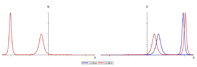
Figure 1. mKdV equation $2$-soliton interaction with $c_{1}/c_{2}=2$, $s_{1}/s_{2}=1$

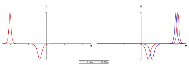
Figure 2. mKdV equation $2$-soliton interaction with $c_{1}/c_{2}=2$, $s_{1}/s_{2}=-1$

In the asymptotic past ($t\rightarrow-\infty$), $\xi_{1}^{-}=0$ gives the position of the peak of the fast soliton, while in the asymptotic future ($t\rightarrow+\infty$), the position of the peak is instead given by $\xi_{1}^{+}=0$. These asymptotic positions lie on straight lines in space-time

$$x=x_{1}+a_{1}^{\mp}+c_{1}t$$ (2.30)

Comparing the asymptotic past with the asymptotic future, we see that the fast soliton retains its shape and speed but gets shifted forward in position as given by

$$\Delta x_{1}=a_{1}^{+}-a_{1}^{-}=\frac{2}{\sqrt{c_{1}}}\ln\left(\frac{\sqrt{c_{1}}+\sqrt{c_{2}}}{\sqrt{c_{1}}-\sqrt{c_{2}}}\right)>0$$ (2.31)

Similarly, the slow soliton retains its shape and speed, while the position of its peak in the asymptotic past and future lies on the straight lines $x=x_{2}+a_{2}^{\mp}+c_{2}t$. So we see that the slow soliton gets shifted backward in position as given by

$$\Delta x_{2}=a_{2}^{+}-a_{2}^{-}=-\frac{2}{\sqrt{c_{2}}}\ln\left(\frac{\sqrt{c_{1}}+\sqrt{c_{2}}}{\sqrt{c_{1}}-\sqrt{c_{2}}}\right)<0$$ (2.32)

The asymptotic shifts (2.31) and (2.32) do not depend on the orientations of the fast and slow solitons. Moreover, these shifts satisfy the relation

$$\sqrt{c_{1}}\Delta x_{1}+\sqrt{c_{2}}\Delta x_{2}=0$$ (2.33)

which can be understood as a consequence of the motion of the center of momentum of the $2$-soliton solution (similarly to the same result known for the KdV 2-soliton solution [14]).

In particular, because $u\simeq u_{1}^{\pm}+u_{2}^{\pm}$ is a superposition as $t\rightarrow\pm\infty$, the conserved mass, momentum and energy of $u$ are given by

$$\mathcal{M}=\mathcal{M}_{1}+\mathcal{M}_{2}=(s_{1}+s_{2})\frac{\pi}{2}$$ (2.34)

$$\mathcal{P}=\mathcal{P}_{1}+\mathcal{P}_{2}=\frac{\sqrt{c_{1}}+\sqrt{c_{2}}}{2}$$ (2.35)

$$\mathcal{E}=\mathcal{E}_{1}+\mathcal{E}_{2}=\frac{\sqrt{c_{1}}^{3}+\sqrt{c_{2}}^{3}}{12}$$ (2.36)

in terms of the mass, momentum and energy individually associated with the fast and slow solitons $u_{1}^{\pm}$ and $u_{2}^{\pm}$. Similarly, the conserved Galilean energy of $u$ is given by

$$\mathcal{C}=\mathcal{C}_{1}+\mathcal{C}_{2}=-\frac{(x_{1}+a_{1}^{-})\sqrt{c_{1}}+(x_{2}+a_{2}^{-})\sqrt{c_{2}}}{12}=-\frac{x_{1}+a_{1}^{+})\sqrt{c_{1}}+(x_{2}+a_{2}^{+})\sqrt{c_{2}}}{12}$$ (2.37)

which simplifies to

$$\mathcal{C}=-\frac{x_{1}\sqrt{c_{1}}+x_{2}\sqrt{c_{2}}}{12}=t\mathcal{E}-\frac{1}{6}\mathcal{P}\mathcal{X}(t)$$ (2.38)

due to the relation $a_{1}^{\pm}\sqrt{c_{1}}+a_{2}^{\pm}\sqrt{c_{2}}=0$. Thus the center of momentum of $u$ is

$$\mathcal{X}(t)=\frac{\sqrt{c_{1}}(x_{1}+c_{1}t)+\sqrt{c_{2}}(x_{2}+c_{2}t)}{\sqrt{c_{1}}+\sqrt{c_{2}}}=\frac{\mathcal{P}_{1}\mathcal{X}_{1}^{\pm}(t)+\mathcal{P}_{2}\mathcal{X}_{2}^{\pm}(t)}{\mathcal{P}_{1}+\mathcal{P}_{2}}$$ (2.39)

where $\mathcal{X}_{1}^{\pm}(t)=x_{1}+a_{1}^{\pm}+c_{1}t$ and $\mathcal{X}_{2}^{\pm}(t)=x_{2}+a_{2}^{\pm}+c_{2}t$ are the respective centers of momentum of the fast and slow solitons in the asymptotic past and future. Therefore, we see that the center of momentum of the $2$-soliton solution moves at constant speed

$$c=\frac{\sqrt{c_{1}}^{3}+\sqrt{c_{2}}^{3}}{\sqrt{c_{1}}+\sqrt{c_{2}}}=\frac{\mathcal{P}_{1}c_{1}+\mathcal{P}_{2}c_{2}}{\mathcal{P}_{1}+\mathcal{P}_{2}}$$ (2.40)

and consequently the asymptotic shifts $\Delta x_{1}$ and $\Delta x_{2}$ in the positions of the two solitons $u_{1}^{\pm}$ and $u_{2}^{\pm}$ are constrained to satisfy $\mathcal{P}_{1}\Delta x_{1}+\mathcal{P}_{2}\Delta x_{2}=0$ which explains the relation (2.33).

2.3. Interaction profile

We now study the interaction profile of the $2$-soliton solution (2.13)–(2.15), which we will write in the equivalent form

$$u(t,x)=\frac{\kappa(s_{1}\sqrt{c_{1}}\cosh(\theta_{2})+s_{2}\sqrt{c_{2}}\cosh(\theta_{1}))}{s_{1}s_{2}(\kappa^{2}-1)+\kappa^{2}\cosh(\theta_{1}-\theta_{2})+\cosh(\theta_{1}+\theta_{2})}$$ (2.41)

in terms of

$$\theta_{1}=\sqrt{c_{1}}\xi_{1},\quad\theta_{2}=\sqrt{c_{2}}\xi_{2}$$ (2.42)

For simplicity, by means of suitable time and space translations $t\rightarrow t-t_{0}$, $x\rightarrow x-x_{0}$, we shift the centers of the moving coordinates (2.17) to the positions

$$x_{1}=x_{0}-c_{1}t_{0}=0,\quad x_{2}=x_{0}-c_{2}t_{0}=0$$ (2.43)

Then the resulting $2$-soliton solution (2.41) is invariant under a combined space-time reflection $x\rightarrow-x$, $t\rightarrow-t$, and its center of momentum is simply $\mathcal{X}(t)=ct$ in terms of the speed (2.40). In the asymptotic past and future ($t\rightarrow\mp\infty$), this solution describes a superposition $u\simeq u_{1}^{\pm}+u_{2}^{\pm}$ of fast and slow solitons $u_{1}^{\pm}$ and $u_{2}^{\pm}$ whose centers of momentum are given by $\mathcal{X}_{1}^{\mp}(t)=a_{1}^{\mp}+c_{1}t$ and $\mathcal{X}_{2}^{\mp}(t)=a_{2}^{\mp}+c_{2}t$ where

$$\Delta\mathcal{X}_{1}^{\mp}(t)=\mathcal{X}_{2}^{\mp}(t)-\mathcal{X}_{1}^{\mp}(t)=\pm\frac{1}{2}(\Delta x_{1}-\Delta x_{2})-(c_{1}-c_{2})t$$ (2.44)

is the separation between the peaks of $u_{1}^{\pm}$ and $u_{2}^{\pm}$ in terms of the asymptotic shifts (2.31) and (2.32) for $t\rightarrow\mp\infty$.

Because of the space-time reflection invariance of $u$, the separation between the fast and slow peaks in $u$ will be a minimum at time $t=0$ when $u$ is an even function of $x$. Qualitatively speaking, $t=0$ will be the moment of greatest nonlinear interaction between the fast and slow solitons. We will therefore refer to the shape of $u$ at $t=0$ as the interaction profile of the $2$-soliton solution. Since this profile $u(0,x)$ is even in $x$, its shape can be characterized by the convexity

$$u(0,x)_{xx}\big{|}_{x=0}=\frac{1}{2}(c_{1}-c_{2})(\sqrt{c_{1}}-\sqrt{c_{2}})(\sqrt{c_{1}c_{2}}-(s_{1}\sqrt{c_{1}}-s_{2}\sqrt{c_{2}})^{2})$$ (2.45)

Note that the sign of the convexity (2.45) depends only on the ratio of speeds and the relative orientation

$$r=c_{1}/c_{2},\quad s=s_{1}/s_{2}$$ (2.46)

of the fast and slow solitons. In particular, since $c_{1}>c_{2}>0$, we have

$$\sigma={\rm sgn}(u(0,x)_{xx}\big{|}_{x=0})={\rm sgn}((2s+1)\sqrt{r}-r-1)$$ (2.47)

with $r>1$ and $s=\pm 1$.

The case where the two solitons have the same orientation is given by the relation $s=1$. In this case, the convexity sign is determined by

$$\sigma={\rm sgn}(3\sqrt{r}-r-1)={\rm sgn}(\tfrac{1}{2}(3+\sqrt{5})-\sqrt{r})$$ (2.48)

via factorization of (2.47) and use of the inequality $r>1$. Hence the sign is indefinite such that

$$\sigma\begin{cases}<0&\hbox{\rm{ if }}r>(7+3\sqrt{5})/2\\ >0&\hbox{\rm{ if }}r<(7+3\sqrt{5})/2\\ =0&\hbox{\rm{ if }}r=(7+3\sqrt{5})/2\\ \end{cases}$$ (2.49)

This result implies that the interaction profile $u(0,x)$ will have either a single peak at $x=0$ if $c_{1}/c_{2}>(7+3\sqrt{5})/2$, or a double peak around $x=0$ if $c_{1}/c_{2}<(7+3\sqrt{5})/2$. These peaks will be positive or negative depending on the sign of $s_{1}$ ($=s_{2}$) and will have an exponentially diminishing tail. In the case of a single peak, the fast and slow solitons interact by first merging together at $t=x=0$ and then splitting apart, while in the case of a double peak, the fast and slow solitons interact by first bouncing and then exchanging shapes and speeds at $t=x=0$. We will call these cases, respectively, a merge-split and bounce-exchange interaction. See Fig. 3 and Fig. 4.

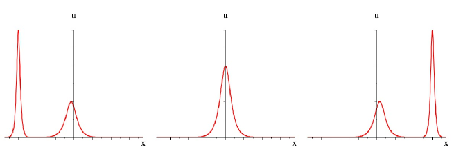
Figure 3. mKdV equation $2$-soliton interaction with $c_{1}/c_{2}=9$, $s_{1}/s_{2}=1$

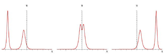
Figure 4. mKdV equation $2$-soliton interaction with $c_{1}/c_{2}=4$, $s_{1}/s_{2}=1$

The value $c_{1}/c_{2}=(7+3\sqrt{5})/2$ which separates these two types of interaction profiles will be called the critical speed ratio.

The other case, where the two solitons have opposite orientations, is given by $s=-1$. In this case, the convexity sign (2.47) is strictly negative for all $r>1$,

$$\sigma=-{\rm sgn}(\sqrt{r}+r+1)<0$$ (2.50)

implying that the interaction profile $u(0,x)$ will have a positive or negative peak at $x=0$ depending on the sign of $s_{1}$ ($=-s_{2}$). Since $s_{2}$ has the opposite sign, the profile will also have a pair of negative or positive side peaks around $x=0$, with an exponentially diminishing tail. The interaction between the fast and slow solitons in this case consists of the slow soliton gradually being first absorbed by the front side of the fast soliton and then emitted from the back side of the fast soliton. We will call this an absorb-emit interaction. See Fig. 5.

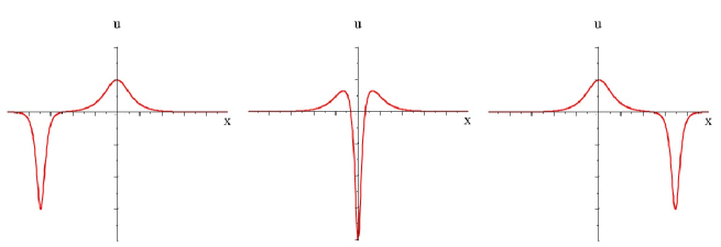
Figure 5. mKdV equation $2$-soliton interaction with $c_{1}/c_{2}=9$, $s_{1}/s_{2}=-1$

3. Hirota-mKdV soliton collisions

For the Hirota equation

$$u_{t}+24|u|^{2}u_{x}+u_{xxx}=0$$ (3.1)

we note, firstly, there is no conserved integral for mass since neither $\int_{-\infty}^{+\infty}u\;dx$ nor $\int_{-\infty}^{+\infty}|u|\;dx$ is a constant of motion. Secondly, we recall the conserved integrals for momentum, energy, and Galilean energy are given by [8]

$$\mathcal{P}=\int_{-\infty}^{+\infty}|u|^{2}\;dx$$ (3.2)

$$\mathcal{E}=\int_{-\infty}^{+\infty}\frac{1}{2}|u_{x}|^{2}-2|u|^{4}\;dx$$ (3.3)

$$\mathcal{C}=\int_{-\infty}^{+\infty}t(\frac{1}{2}|u_{x}|^{2}-2|u|^{4})-x\frac{1}{6}|u|^{2}\;dx$$ (3.4)

which are constants of motion for all smooth solutions $u(t,x)$ with asymptotic decay $u\rightarrow 0$ as $x\rightarrow\pm\infty$. These integrals are related to the center of momentum

$$\mathcal{X}(t)=\frac{1}{\mathcal{P}}\int_{-\infty}^{+\infty}x|u|^{2}\;dx=\mathcal{X}(0)+6\frac{\mathcal{E}}{\mathcal{P}}t$$ (3.5)

since

$$\mathcal{C}=t\mathcal{E}-\frac{1}{6}\mathcal{P}\mathcal{X}(t)=\mathcal{C}(0)=-\frac{1}{6}\mathcal{P}\mathcal{X}(0)$$ (3.6)

This is the same relation that holds for the mKdV constants of motion.

The $1$-soliton solution for the Hirota equation is given by

$$u(t,x)=\frac{\sqrt{c}}{2}\exp(i\phi){\rm sech}\left(\sqrt{c}\xi\right)=\frac{\sqrt{c}\exp(i\phi+\sqrt{c}\xi)}{1+\exp(2\sqrt{c}\xi)}$$ (3.7)

with speed $c>0$ and phase $-\pi\leq\phi\leq\pi$, where

$$\xi=x-ct$$ (3.8)

is a moving coordinate. This solution describes a stable uni-directional travelling wave whose amplitude $|u|$ is the same as the amplitude of the mKdV solitary wave (2.8). Therefore, its constants of motion (3.2)–(3.4) and its center of momentum (3.5) are also the same as those for the mKdV solitary wave. In particular, the position of the peak amplitude coincides with the center of momentum $\mathcal{X}(t)=ct$, which can be shifted arbitrarily by means of a space translation

$$x\rightarrow x-x_{0}$$ (3.9)

applied to the moving coordinate (3.8).

3.1. $2$-soliton solution

We now write down the $2$-soliton solution of the Hirota equation describing collisions where a fast soliton with speed $c_{1}$ and phase $\phi_{1}$ overtakes a slow soliton with speed $c_{2}$ and phase $\phi_{2}$. (See the animations of collisions at http://lie.math.brocku.ca/~sanco/solitons/hirota.php ) This solution has the rational-exponential form (2.13) given by [9]

$$G= \kappa\big{(}\sqrt{c_{1}}\exp(i\phi_{1}+\sqrt{c_{1}}\xi_{1})(1+\exp(2\sqrt{c_{2}}\xi_{2}))+\sqrt{c_{2}}\exp(i\phi_{2}+\sqrt{c_{2}}\xi_{2})(1+\exp(2\sqrt{c_{1}}\xi_{1}))\big{)}$$ (3.10)

$$F= 1+2\cos(\phi_{1}-\phi_{2})(\kappa^{2}-1)\exp(\sqrt{c_{1}}\xi_{1}+\sqrt{c_{2}}\xi_{2})+\kappa^{2}(\exp(2\sqrt{c_{1}}\xi_{1})+\exp(2\sqrt{c_{2}}\xi_{2}))$$

$$\qquad+\exp(2(\sqrt{c_{1}}\xi_{1}+\sqrt{c_{2}}\xi_{2}))$$ (3.11)

in terms of

$$\kappa=\frac{\sqrt{c_{1}}+\sqrt{c_{2}}}{\sqrt{c_{1}}-\sqrt{c_{2}}}>1$$ (3.12)

where

$$\xi_{1}=x-c_{1}t-x_{1},\quad\xi_{2}=x-c_{2}t-x_{2}$$ (3.13)

are moving coordinates centered at initial positions $x=x_{1}$ and $x=x_{2}$ respectively.

The asymptotic form of the $2$-soliton solution $u(t,x)=G/F$ as $t\rightarrow\pm\infty$ is easily derived by the same moving-coordinate expansions considered for the mKdV $2$-soliton solution. These expansions yield, after neglecting subdominant exponential terms,

$$u(t,x)\simeq\frac{\sqrt{c_{1}}\exp(i\phi_{1}+\sqrt{c_{1}}(\xi_{1}-a_{1}^{\pm}))}{1+\exp(2\sqrt{c_{1}}(\xi_{1}-a_{1}^{\pm}))}=u_{1}^{\pm},\quad t\rightarrow\pm\infty,\quad\xi_{1}={\rm const.}$$ (3.14)

and

$$u(t,x)\simeq\frac{\sqrt{c_{2}}\exp(i\phi_{2}+\sqrt{c_{2}}(\xi_{2}-a_{2}^{\pm}))}{1+\exp(2\sqrt{c_{2}}(\xi_{2}-a_{2}^{\pm}))}=u_{2}^{\pm},\quad t\rightarrow\pm\infty,\quad\xi_{2}={\rm const.}$$ (3.15)

where $a_{1}^{\pm},a_{2}^{\pm}$ are shifts in the moving coordinates $\xi_{1},\xi_{2}$ given by (2.23) and (2.29) respectively.

Thus, the $2$-soliton solution (2.13) and (3.10)–(3.11) asymptotically has the form of a superposition $u\simeq u_{1}^{\pm}+u_{2}^{\pm}$ for $t\rightarrow\pm\infty$, where $u_{1}^{\pm}$ is a fast soliton (3.7) with speed $c_{1}$ and phase $\phi_{1}$ and where $u_{2}^{\pm}$ is a slow soliton (3.7) with speed $c_{2}$ and phase $\phi_{2}$, whose positions are determined by the shifted moving coordinates (2.22) and (2.28). This solution has the same conserved momentum (2.35), energy (2.36), Galilean energy (2.38), and center of momentum (2.39) as the mKdV $2$-soliton solution.

3.2. Asymptotic position shifts

For the $2$-soliton solution $u$ of the Hirota equation, the asymptotic expansions (3.14) and (3.15) for $t\rightarrow-\infty$ compared to $t\rightarrow+\infty$ show that the fast soliton $u_{1}$ retains its shape, speed and phase, but gets shifted forward in position by

$$\Delta x_{1}=a_{1}^{+}-a_{1}^{-}=\frac{2}{\sqrt{c_{1}}}\ln\left(\frac{\sqrt{c_{1}}+\sqrt{c_{2}}}{\sqrt{c_{1}}-\sqrt{c_{2}}}\right)>0$$ (3.16)

while the slow soliton $u_{2}$ similarly retains its shape, speed and phase, but gets shifted backward in position by

$$\Delta x_{2}=a_{2}^{+}-a_{2}^{-}=-\frac{2}{\sqrt{c_{2}}}\ln\left(\frac{\sqrt{c_{1}}+\sqrt{c_{2}}}{\sqrt{c_{1}}-\sqrt{c_{2}}}\right)<0$$ (3.17)

These expressions are the same asymptotic shifts seen for the collision of mKdV solitons. In particular, the shifts (3.16) and (3.17) here are independent of the phases of the fast and slow solitons and also satisfy the center of momentum relations (2.33) and (2.44).

3.3. Interaction profile

In the same way as for the mKdV $2$-soliton solution, we will now write the Hirota $2$-soliton solution given by (2.13) and (3.10)–(3.11) in the equivalent rational-cosh form

$$u(t,x)=\frac{\kappa(\sqrt{c_{1}}\exp(i\phi_{1})\cosh(\theta_{2})+\sqrt{c_{2}}\exp(i\phi_{2})\cosh(\theta_{1}))}{(\kappa^{2}-1)\cos(\phi_{1}-\phi_{2})+\kappa^{2}\cosh(\theta_{1}-\theta_{2})+\cosh(\theta_{1}+\theta_{2})}$$ (3.18)

with

$$\theta_{1}=\sqrt{c_{1}}\xi_{1},\quad\theta_{2}=\sqrt{c_{2}}\xi_{2}$$ (3.19)

By shifting the centers of the moving coordinates (3.13) to the positions

$$x_{1}=x_{0}-c_{1}t_{0}=0,\quad x_{2}=x_{0}-c_{2}t_{0}=0,$$ (3.20)

we then see that the resulting solution (3.18) of the Hirota equation is invariant under the combined space-time reflection $x\rightarrow-x$, $t\rightarrow-t$. As a consequence, this solution $u$ describes a collision of fast and slow solitons $u_{1}^{\pm}$ and $u_{2}^{\pm}$ whose separation will be a minimum at time $t=0$ when the amplitude $|u|$ is an even function of $x$. This can be understood to be the moment of greatest nonlinear interaction between the fast and slow solitons in the collision. The shape of $|u|$ at $t=0$ therefore defines the interaction profile of the $2$-soliton solution $u$. Since this profile is even in $x$, its shape is characterized by the convexity of $|u(0,x)|$ at $x=0$. An explicit calculation of the convexity yields

$$|u(0,x)|_{xx}\big{|}_{x=0}=\frac{(\sqrt{c_{1}}-\sqrt{c_{2}})^{2}(4c_{1}c_{2}-c_{1}^{2}-c_{2}^{2}+\sqrt{c_{1}c_{2}}(c_{1}+c_{2})\cos(\phi_{1}-\phi_{2}))}{2(c_{1}+c_{2}+2\sqrt{c_{1}c_{2}}\cos(\phi_{1}-\phi_{2}))^{3/2}}$$ (3.21)

The sign of the convexity (3.21) depends only on the ratio of speeds and the relative phase

$$r=c_{1}/c_{2},\quad\Delta\phi=\phi_{1}-\phi_{2}\mod 2\pi$$ (3.22)

of the fast and slow solitons. In particular, since $c_{1}>c_{2}>0$, we have

$$\sigma={\rm sgn}(|u(0,x)|_{xx}\big{|}_{x=0})={\rm sgn}(4r-r^{2}-1+\sqrt{r}(r+1)\cos\Delta\phi)$$ (3.23)

with $r>1$ and $-\pi\leq\Delta\phi\leq\pi$. This expression (3.23) is a quartic polynomial in $\sqrt{r}$. By factorizing

$$4r-r^{2}-1+\sqrt{r}(r+1)\cos\Delta\phi=$$

$$\qquad\big{(}\tfrac{1}{2}(\cos\Delta\phi+\sqrt{\cos^{2}\Delta\phi+24})\sqrt{r}-r-1\big{)}\big{(}\tfrac{1}{2}(\cos\Delta\phi+\sqrt{\cos^{2}\Delta\phi+24})\sqrt{r}+r+1\big{)}$$

and using the inequality

$$\sqrt{\cos^{2}\Delta\phi+24}>\pm\cos\Delta\phi$$

we obtain

$$\sigma={\rm sgn}(\tfrac{1}{2}(\cos\Delta\phi+\sqrt{\cos^{2}\Delta\phi+24})\sqrt{r}-r-1)$$ (3.24)

which is a quadratic polynomial in $\sqrt{r}$ with two real positive roots

$$\sqrt{r_{\pm}}=\tfrac{1}{4}(\cos\Delta\phi+\sqrt{\cos^{2}\Delta\phi+24})\pm\sqrt{(\tfrac{1}{4}(\cos\Delta\phi+\sqrt{\cos^{2}\Delta\phi+24}))^{2}-1}\ >0$$ (3.25)

These roots satisfy $r_{+}r_{-}=1$, where the case $r_{+}=r_{-}=1$ occurs iff $|\Delta\phi|=\pi$. Hence we have

$$r_{+}\geq 1\geq r_{-}$$ (3.26)

in all cases. Thus the convexity sign (3.24) is determined by

$$\sigma={\rm sgn}(\sqrt{r_{+}}-\sqrt{r})$$ (3.27)

which is indefinite such that

$$\sigma\begin{cases}<0&\hbox{\rm{ if }}r>r_{+}\\ >0&\hbox{\rm{ if }}r<r_{+}\\ =0&\hbox{\rm{ if }}r=r_{+}\\ \end{cases}$$ (3.28)

where

$$r_{+}=2+\tfrac{1}{4}\big{(}\cos\Delta\phi+\sqrt{\cos^{2}\Delta\phi+24}\ \big{)}\big{(}\cos\Delta\phi+\sqrt{\tfrac{1}{2}(\cos\Delta\phi+\sqrt{\cos^{2}\Delta\phi+24})\cos\Delta\phi+2}\ \big{)}$$ (3.29)

The result (3.28) implies that the $2$-soliton interaction profile $|u(0,x)|$ will have either a single peak at $x=0$ if $c_{1}/c_{2}>r_{+}$ or a double peak around $x=0$ if $c_{1}/c_{2}<r_{+}$, as determined by the critical speed ratio (3.29) in terms of the relative phase angle $\Delta\phi$.

In the case of a single peak, the profile has one of two different shapes depending on whether $|\Delta\phi|$ is greater than or less than a certain critical value given by some function of $c_{1}/c_{2}$ that is determined by the conditions $|u(0,x)|_{xx}=|u(0,x)|_{x}=0$ for existence of a saddle point at some $x\neq 0$ (which we can solve for numerically). For $|\Delta\phi|$ below the critical value, the shape of $|u(0,x)|$ is simply a single peak with an exponentially diminishing tail. In this case the fast and slow solitons undergo a merge-split interaction, i.e. where they first merge together at $t=x=0$ and then split apart: See Fig. 6 and Fig. 7. For $|\Delta\phi|$ above the critical value, the shape of $|u(0,x)|$ consists of a pair of side peaks around the main peak at $x=0$. In this case the fast and slow solitons undergo an absorb-emit interaction, i.e. where the slow soliton gradually is first absorbed by the front side of the fast soliton and is then emitted from the back side of the fast soliton. See Fig. 8 and Fig. 9.

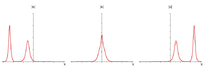
Figure 6. Hirota equation $2$-soliton interaction with $c_{1}/c_{2}=3$, $\phi_{1}-\phi_{2}=0.855\pi$

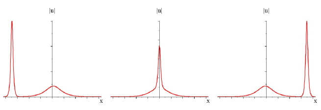
Figure 7. Hirota equation $2$-soliton interaction with $c_{1}/c_{2}=50$, $\phi_{1}-\phi_{2}=0.3\pi$

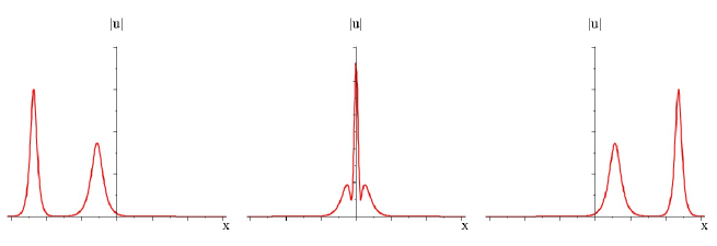
Figure 8. Hirota equation $2$-soliton interaction with $c_{1}/c_{2}=3$, $\phi_{1}-\phi_{2}=0.855\pi$

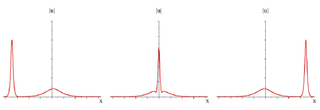
Figure 9. Hirota equation $2$-soliton interaction with $c_{1}/c_{2}=50$, $\phi_{1}-\phi_{2}=0.855\pi$

The interaction in the special case when $|\Delta\phi|$ equals the critical value is shown in Fig. 10.

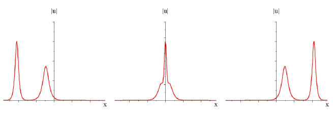
Figure 10. Hirota equation $2$-soliton interaction with $c_{1}/c_{2}=3$, $\phi_{1}-\phi_{2}=0.85598\pi$

In contrast, in the case of a double peak, the profile $|u(0,x)|$ always has an exponentially diminishing tail, regardless of the relative phase angle $|\Delta\phi|$. This case describes the fast and slow solitons undergoing a bounce-exchange interaction, i.e. where they first bounce and then exchange shapes and speeds at $t=x=0$: See Fig. 11.

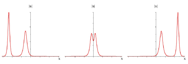
Figure 11. Hirota equation $2$-soliton interaction with $c_{1}/c_{2}=3$, $\phi_{1}-\phi_{2}=0.3\pi$

The range of values of $c_{1}/c_{2}$ and $|\Delta\phi|$ that characterize these three different types of interaction is shown in Fig. 12.

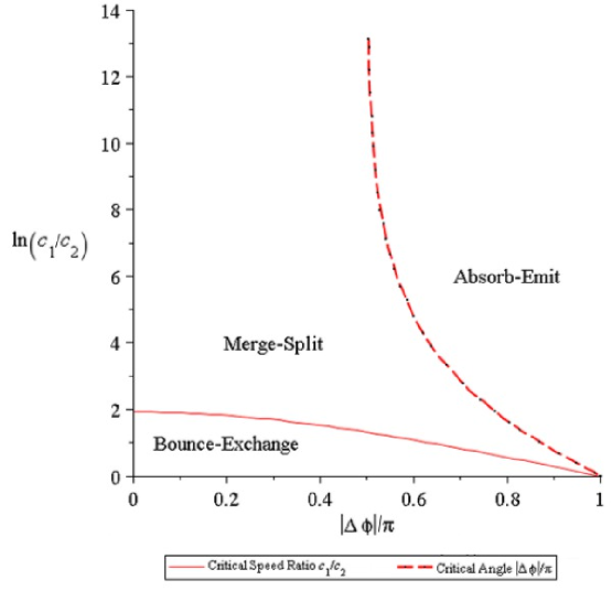
Figure 12. Types of $2$-soliton interactions for the Hirota equation

4. Sasa-Satsuma-mKdV soliton collisions

For the Sasa-Satsuma equation

$$u_{t}+6(u\bar{u}_{x}+3u_{x}\bar{u})u+u_{xxx}=0$$ (4.1)

we begin by remarking [8] that it has the same conserved integrals as the Hirota equation for momentum (3.2), energy (3.3), and Galilean energy (3.4), which define constants of motion for all smooth solutions $u(t,x)$ with asymptotic decay $u\rightarrow 0$ as $x\rightarrow\pm\infty$. In addition these integrals have the same relation to the center of momentum (3.5)–(3.6) that holds for the Hirota equation.

The $1$-soliton solution for the Sasa-Satsuma equation has the same form (3.7)–(3.8) as the Hirota $1$-soliton with speed $c>0$ and phase $-\pi\leq\phi\leq\pi$. We recall that this solution describes a stable uni-directional travelling wave $u$ whose amplitude $|u|$ is the same as the amplitude of the mKdV solitary wave (2.8), and hence $u$ also has the same constants of motion (3.2)–(3.4) and center of momentum (3.5) as those of the mKdV solitary wave. Thus, the position of the peak amplitude of $u$ coincides with the center of momentum $\mathcal{X}(t)=ct$ which can be shifted arbitrarily via a space translation $x\rightarrow x-x_{0}$ applied to the moving coordinate (3.8), yielding

$$u(t,x)=\frac{\sqrt{c}}{2}\exp(i\phi){\rm sech}\left(\sqrt{c}\xi\right)=\frac{\sqrt{c}\exp(i\phi+\sqrt{c}\xi)}{1+\exp(2\sqrt{c}\xi)}$$ (4.2)

with

$$\xi=x-ct-x_{0}$$ (4.3)

4.1. $2$-soliton solution

The $2$-soliton solution of the Sasa-Satsuma equation describing collisions where a fast soliton with speed $c_{1}$ and phase $\phi_{1}$ overtakes a slow soliton with speed $c_{2}$ and phase $\phi_{2}$ has not appeared previously in an explicit form [15]. We give a simple derivation of this solution in the appendix, based on using a rational-exponential ansatz similar to the form of the $2$-soliton solution of the Hirota equation. This derivation yields

$$u(t,x)=\frac{G}{F}$$ (4.4)

with

$$G= \frac{\rho}{\sqrt{\gamma}}\Big{(}\sqrt{c_{1}}\exp(i\phi_{1}+\sqrt{c_{1}}\xi_{1})\big{(}(\sqrt{c_{1}}+\sqrt{c_{2}}\exp(2i(\phi_{2}-\phi_{1})))\exp(2\sqrt{c_{2}}\xi_{2})+\gamma\big{)}$$

$$\qquad+\sqrt{c_{2}}\exp(i\phi_{2}+\sqrt{c_{2}}\xi_{2})\big{(}\gamma\exp(2\sqrt{c_{1}}\xi_{1})+\sqrt{c_{2}}+\sqrt{c_{1}}\exp(2i(\phi_{1}-\phi_{2}))\big{)}\Big{)}$$ (4.5)

$$F= 1+2\cos(\phi_{1}-\phi_{2})((\sqrt{c_{1}}+\sqrt{c_{2}})\rho^{2}-1)\exp(\sqrt{c_{1}}\xi_{1}+\sqrt{c_{2}}\xi_{2})$$

$$\qquad+\gamma\rho^{2}(\exp(2\sqrt{c_{1}}\xi_{1})+\exp(2\sqrt{c_{2}}\xi_{2}))+\exp(2(\sqrt{c_{1}}\xi_{1}+\sqrt{c_{2}}\xi_{2}))$$ (4.6)

in terms of

$$\rho=\frac{\sqrt{\sqrt{c_{1}}+\sqrt{c_{2}}}}{\sqrt{c_{1}}-\sqrt{c_{2}}}>0$$ (4.7)

and

$$\gamma=|\sqrt{c_{1}}\exp(i(\phi_{2}-\phi_{1}))+\sqrt{c_{2}}\exp(i(\phi_{1}-\phi_{2}))|=\sqrt{c_{1}+c_{2}+2\sqrt{c_{1}c_{2}}\cos 2(\phi_{1}-\phi_{2})}>0$$ (4.8)

where

$$\xi_{1}=x-c_{1}t-x_{1},\quad\xi_{2}=x-c_{2}t-x_{2}$$ (4.9)

are moving coordinates centered at initial positions $x=x_{1}$ and $x=x_{2}$ respectively. (See the animations of collisions at http://lie.math.brocku.ca/~sanco/solitons/sasa-satsuma.php )

We will now examine the asymptotic form of the $2$-soliton solution (4.4)–(4.6) as $t\rightarrow\pm\infty$ by means of the same moving-coordinate expansions used for the mKdV $2$-soliton solution.

First we hold $\xi_{1}$ fixed and asymptotically expand $F$ and $G$ for large $\zeta=t\Delta c-\Delta x$ with $\xi_{2}=\xi_{1}+\zeta$. This yields, after neglecting subdominant exponential terms,

$$G\simeq\begin{cases}\dfrac{\rho}{\sqrt{\gamma}}\sqrt{c_{1}}\exp(i\phi_{1}+(\sqrt{c_{1}}+2\sqrt{c_{2}})\xi_{1})(\sqrt{c_{1}}+\sqrt{c_{2}}\exp(2i(\phi_{2}-\phi_{1})))\exp(2\sqrt{c_{2}}\zeta)&\zeta\rightarrow+\infty\\ \rho\sqrt{\gamma}\sqrt{c_{1}}\exp(i\phi_{1}+\sqrt{c_{1}}\xi_{1})&\zeta\rightarrow-\infty\end{cases}$$ (4.10)

$$F\simeq\begin{cases}\big{(}\gamma\rho^{2}\exp(2\sqrt{c_{2}}\xi_{1})+\exp(2(\sqrt{c_{1}}+\sqrt{c_{2}})\xi_{1})\big{)}\exp(2\sqrt{c_{2}}\zeta)&\zeta\rightarrow+\infty\\ 1+\gamma\rho^{2}\exp(2\sqrt{c_{1}}\xi_{1})&\zeta\rightarrow-\infty\end{cases}$$ (4.11)

and hence we obtain the expansion

$$u\simeq\begin{cases}\dfrac{(\sqrt{c_{1}}/\rho\sqrt{\gamma^{3}})\exp(i\phi_{1}+\sqrt{c_{1}}\xi_{1})(\sqrt{c_{1}}+\sqrt{c_{2}}\exp(2i(\phi_{2}-\phi_{1})))}{1+(1/\rho^{2}\gamma)\exp(2\sqrt{c_{1}}\xi_{1})}&\zeta\rightarrow+\infty\\ \dfrac{\sqrt{c_{1}}\rho\sqrt{\gamma}\exp(i\phi_{1}+\sqrt{c_{1}}\xi_{1})}{1+\rho^{2}\gamma\exp(2\sqrt{c_{1}}\xi_{1})}&\zeta\rightarrow-\infty\end{cases}$$ (4.12)

where $\zeta\rightarrow\pm\infty$ corresponds to $t\rightarrow\pm\infty$. In the asymptotic past, this expansion (4.12) has the form of a $1$-soliton solution

$$u\simeq\frac{\sqrt{c_{1}}\exp(i\phi_{1}+\sqrt{c_{1}}(\xi_{1}-a_{1}^{-}))}{1+\exp(2\sqrt{c_{1}}(\xi_{1}-a_{1}^{-}))}=u_{1}^{-},\quad t\rightarrow-\infty,\quad\xi_{1}={\rm const.}$$ (4.13)

in which the moving coordinate $\xi_{1}$ is shifted by

$$a_{1}^{-}=-\ln(\rho\sqrt{\gamma})/\sqrt{c_{1}}$$ (4.14)

Similarly, in the asymptotic future, the expansion (4.12) again has the form of a $1$-soliton solution

$$u\simeq\frac{\sqrt{c_{1}}\exp(i(\phi_{1}+\nu_{1})+\sqrt{c_{1}}(\xi_{1}-a_{1}^{+}))}{1+\exp(2\sqrt{c_{1}}(\xi_{1}-a_{1}^{+}))}=u_{1}^{+},\quad t\rightarrow+\infty,\quad\xi_{1}={\rm const.}$$ (4.15)

in which the moving coordinate $\xi_{1}$ is now shifted by

$$a_{1}^{+}=\ln(\rho\sqrt{\gamma})/\sqrt{c_{1}}$$ (4.16)

while in addition there is a phase shift given by

$$\frac{\sqrt{c_{1}}+\sqrt{c_{2}}\exp(2i(\phi_{2}-\phi_{1}))}{\gamma}=\exp(i\nu_{1})$$ (4.17)

where

$$\nu_{1}=\arctan\left(\dfrac{\sqrt{c_{2}}\sin 2(\phi_{1}-\phi_{2})}{\sqrt{c_{1}}+\sqrt{c_{2}}\cos 2(\phi_{1}-\phi_{2})}\right)$$ (4.18)

Second we hold $\xi_{2}$ fixed and asymptotically expand $F$ and $G$ for large $\zeta=t\Delta c-\Delta x$ with $\xi_{1}=\xi_{2}-\zeta$. After neglecting subdominant exponential terms, we obtain

$$G\simeq\begin{cases}\dfrac{\rho}{\sqrt{\gamma}}\sqrt{c_{2}}\exp(i\phi_{2}+\sqrt{c_{2}}\xi_{2})\big{(}\sqrt{c_{2}}+\sqrt{c_{1}}\exp(2i(\phi_{1}-\phi_{2}))\big{)}&\zeta\rightarrow+\infty\\ \rho\sqrt{\gamma}\sqrt{c_{2}}\exp(i\phi_{2}+(\sqrt{c_{2}}+2\sqrt{c_{1}})\xi_{2})\exp(-2\sqrt{c_{1}}\zeta)&\zeta\rightarrow-\infty\end{cases}$$ (4.19)

$$F\simeq\begin{cases}1+\gamma\rho^{2}\exp(2\sqrt{c_{2}}\xi_{2})&\zeta\rightarrow+\infty\\ \big{(}\gamma\rho^{2}\exp(2\sqrt{c_{1}}\xi_{2})+\exp(2(\sqrt{c_{1}}+\sqrt{c_{2}})\xi_{2})\big{)}\exp(-2\sqrt{c_{1}}\zeta)&\zeta\rightarrow-\infty\end{cases}$$ (4.20)

which yields the expansion

$$u\simeq\begin{cases}\dfrac{(\sqrt{c_{2}}/\rho/\sqrt{\gamma})\exp(i\phi_{2}+\sqrt{c_{2}}\xi_{2})(\sqrt{c_{2}}+\sqrt{c_{1}}\exp(2i(\phi_{1}-\phi_{2})))}{1+\rho^{2}\gamma\exp(2\sqrt{c_{2}}\xi_{2})}&\zeta\rightarrow+\infty\\ \dfrac{(\sqrt{c_{2}}/\rho\sqrt{\gamma})\exp(i\phi_{2}+\sqrt{c_{2}}\xi_{2})}{1+(1/\rho^{2}\gamma)\exp(2\sqrt{c_{2}}\xi_{2})}&\zeta\rightarrow-\infty\end{cases}$$ (4.21)

where $\zeta\rightarrow\pm\infty$ corresponds to $t\rightarrow\pm\infty$. In the asymptotic past, the expansion (4.21) has the form of a $1$-soliton solution

$$u\simeq\frac{\sqrt{c_{2}}\exp(i\phi_{2}+\sqrt{c_{2}}(\xi_{2}-a_{2}^{-}))}{1+\exp(2\sqrt{c_{2}}(\xi_{2}-a_{2}^{-}))}=u_{2}^{-},\quad t\rightarrow-\infty,\quad\xi_{2}={\rm const.}$$ (4.22)

in which the moving coordinate $\xi_{2}$ is shifted by

$$a_{2}^{-}=\ln(\rho\sqrt{\gamma})/\sqrt{c_{2}}$$ (4.23)

In the asymptotic future, this expansion (4.21) similarly has the form of a $1$-soliton solution

$$u\simeq\frac{\sqrt{c_{2}}\exp(i(\phi_{2}+\nu_{2})+\sqrt{c_{2}}(\xi_{2}-a_{2}^{+}))}{1+\exp(2\sqrt{c_{2}}(\xi_{2}-a_{2}^{+}))}=u_{2}^{+},\quad t\rightarrow+\infty,\quad\xi_{2}={\rm const.}$$ (4.24)

in which the moving coordinate $\xi_{2}$ is now shifted by

$$a_{2}^{+}=-\ln(\rho\sqrt{\gamma})/\sqrt{c_{2}}$$ (4.25)

while in addition there is a phase shift given by

$$\frac{\sqrt{c_{2}}+\sqrt{c_{1}}\exp(2i(\phi_{1}-\phi_{2}))}{\gamma}=\exp(i\nu_{2})$$ (4.26)

where

$$\nu_{2}=\arctan\left(\dfrac{\sqrt{c_{1}}\sin 2(\phi_{2}-\phi_{1})}{\sqrt{c_{2}}+\sqrt{c_{1}}\cos 2(\phi_{2}-\phi_{1})}\right)$$ (4.27)

Thus, for $t\rightarrow\pm\infty$, the $2$-soliton solution (4.4)–(4.6) asymptotically has the form of a superposition $u\simeq u_{1}^{\pm}+u_{2}^{\pm}$ of a fast soliton $u_{1}^{\pm}$ and a slow soliton $u_{2}^{\pm}$, with speeds $c_{1}$ and $c_{2}$. As a consequence, this solution has the same conserved momentum (2.35), energy (2.36), Galilean energy (2.38), and center of momentum (2.39) as the mKdV $2$-soliton solution.

4.2. Asymptotic position and phase shifts

In the $2$-soliton solution $u$ of the Sasa-Satsuma equation, the positions of the fast soliton $u_{1}^{\pm}$ and the slow soliton $u_{2}^{\pm}$ in the asymptotic past ($t\rightarrow-\infty$) and future ($t\rightarrow+\infty$) are determined by the shifted moving coordinates $\xi_{1}^{\pm}=\xi_{1}-a_{1}^{\pm}$ and $\xi_{2}^{\pm}=\xi_{2}-a_{2}^{\pm}$. We thus see that the fast soliton $u_{1}$ retains its shape and speed, but gets shifted forward in position by

$$\Delta x_{1}=a_{1}^{+}-a_{1}^{-}=\frac{1}{\sqrt{c_{1}}}\ln\left(\frac{(\sqrt{c_{1}}+\sqrt{c_{2}})\sqrt{c_{1}+c_{2}+2\sqrt{c_{1}c_{2}}\cos 2(\phi_{1}-\phi_{2})}}{(\sqrt{c_{1}}-\sqrt{c_{2}})^{2}}\right)>0$$ (4.28)

while the slow soliton $u_{2}$ similarly retains its shape and speed, but gets shifted backward in position by

$$\Delta x_{2}=a_{2}^{+}-a_{2}^{-}=-\frac{1}{\sqrt{c_{2}}}\ln\left(\frac{(\sqrt{c_{1}}+\sqrt{c_{2}})\sqrt{c_{1}+c_{2}+2\sqrt{c_{1}c_{2}}\cos 2(\phi_{1}-\phi_{2})}}{(\sqrt{c_{1}}-\sqrt{c_{2}})^{2}}\right)<0$$ (4.29)

These asymptotic shifts satisfy the relation

$$\sqrt{c_{1}}\Delta x_{1}+\sqrt{c_{2}}\Delta x_{2}=0$$ (4.30)

which can be understood as a consequence of the motion of the center of momentum of the $2$-soliton solution $u$ in the same way as for the Hirota equation. Interestingly, in contrast to collisions of Hirota solitons, here the shifts (4.28) and (4.29) depend on the relative phase angle $\phi_{1}-\phi_{2}$ between the fast and slow solitons in the collision.

Even more interestingly, in the collision, both the fast and slow solitons undergo a shift in phase given by (4.18) and (4.27) respectively. The features of these asymptotic shifts can be understood from the reflection properties of the $2$-soliton solution as follows. First we write this solution in the equivalent form

$$u(t,x)=\frac{\rho\sqrt{\gamma}\big{(}\sqrt{c_{1}}\exp(i\phi_{1})(\exp(-\theta_{2})+\exp(i\nu_{1}+\theta_{2}))+\sqrt{c_{2}}\exp(i\phi_{2})(\exp(\theta_{1})+\exp(i\nu_{2}-\theta_{1}))\big{)}}{2\big{(}\cosh(\theta_{1}+\theta_{2})+\rho^{2}\gamma\cosh(\theta_{1}-\theta_{2})+\cos(\phi_{1}-\phi_{2})((\sqrt{c_{1}}+\sqrt{c_{2}})\rho^{2}-1)\big{)}}$$ (4.31)

with

$$\theta_{1}=\sqrt{c_{1}}(x-c_{1}t),\quad\theta_{2}=\sqrt{c_{2}}(x-c_{2}t),$$ (4.32)

where we have used a space-time translation $x\rightarrow x-x_{0}$ and $t\rightarrow t-t_{0}$ to shift the centers of the moving coordinates (4.9) to the positions

$$x_{1}=x_{0}-c_{1}t_{0}=0,\quad x_{2}=x_{0}-c_{2}t_{0}=0$$ (4.33)

The solution (4.31) of the Sasa-Satsuma equation then exhibits an invariance

$$u(-t,-x)=\exp(i\nu){\bar{u}}(t,x)$$ (4.34)

where the phase factor is given by

$$\exp(i\nu)=\frac{\sqrt{c_{2}}\exp(i\phi_{1})+\sqrt{c_{1}}\exp(i\phi_{2})}{\gamma}=\exp(i(\nu_{1}+2\phi_{1}))=\exp(i(\nu_{2}+2\phi_{2}))$$ (4.35)

in terms of the asymptotic phase shifts $\nu_{1}$ and $\nu_{2}$. Next we shift the phases

$$\phi_{1}\rightarrow\phi_{1}-\nu/2,\quad\phi_{2}\rightarrow\phi_{2}-\nu/2$$ (4.36)

which corresponds to an overall phase rotation of the solution

$$u\rightarrow\exp(-i\nu/2)u=\hat{u}$$ (4.37)

This does not affect the relative phase angle $\phi_{1}-\phi_{2}$ between the fast and slow solitons in the collision, whereby the resulting solution

$${\hat{u}}(t,x)=\frac{\rho\sqrt{\gamma}\big{(}\sqrt{c_{1}}\cosh(\theta_{2}+i\nu_{1}/2)+\sqrt{c_{2}}\cosh(\theta_{1}-i\nu_{2}/2)\big{)}}{\big{(}\cosh(\theta_{1}+\theta_{2})+\rho^{2}\gamma\cosh(\theta_{1}-\theta_{2})+\cos(\phi_{1}-\phi_{2})((\sqrt{c_{1}}+\sqrt{c_{2}})\rho^{2}-1)\big{)}}$$ (4.38)

is invariant under space-time reflection $x\rightarrow-x$, $t\rightarrow-t$, combined with phase conjugation,

$${\hat{u}}(-t,-x)=\bar{\hat{u}}(t,x)$$ (4.39)

For $t\rightarrow\pm\infty$, this $2$-soliton solution $\hat{u}$ of the Sasa-Satsuma equation describes a collision where, in the asymptotic past ($t\rightarrow-\infty$), a fast soliton $\hat{u}_{1}^{-}$ with speed $c_{1}$, phase $\phi_{1}^{-}=\phi_{1}-\nu/2=-nu_{1}/2$, and center of momentum $\chi_{1}^{-}(t)=a_{1}^{-}+c_{1}t$ overtakes a slow soliton $\hat{u}_{2}^{-}$ with speed $c_{2}$, phase $\phi_{2}^{-}=\phi_{2}-\nu/2=-\nu_{2}/2$, and center of momentum $\chi_{2}^{-}(t)=a_{2}^{-}+c_{2}t$. In the asymptotic future ($t\rightarrow+\infty$), the fast soliton $\hat{u}_{1}^{+}$ undergoes a shift in both position $\chi_{1}^{+}(t)=a_{1}^{+}+c_{1}t$ and phase $\phi_{1}^{+}=\nu_{1}+\phi_{1}^{-}=\nu_{1}/2$, while the slow soliton $\hat{u}_{2}^{+}$ similarly undergoes both a position shift $\chi_{2}^{+}(t)=a_{2}^{+}+c_{2}t$ and a phase shift $\phi_{2}^{+}=\nu_{2}+\phi_{2}^{-}=\nu_{2}/2$, where these phase shifts are related by

$$\phi_{1}^{-}-\phi_{2}^{-}=-(\phi_{1}^{+}-\phi_{2}^{+})$$ (4.40)

due to the reflection property (4.39).

This asymptotic phase relation (4.40) is equivalent to

$$\nu_{1}-\nu_{2}=-2(\phi_{1}-\phi_{2})$$ (4.41)

Thus, surprisingly, the relative phase angle between the fast and slow solitons is not preserved in the collision but instead changes sign.

4.3. Interaction profile

The invariance property (4.34) of the $2$-soliton solution $u$ shows that the separation in positions of the peak amplitude of the fast and slow solitons $u_{1}^{\pm}$ and $u_{2}^{\pm}$ in the collision will be a minimum at time $t=0$ when the amplitude $|u|$ is an even function of $x$. The shape of $|u|$ at $t=0$ thereby defines the interaction profile of the $2$-soliton solution $u$, which can be understood to be the moment of greatest nonlinear interaction between the fast and slow solitons in the collision. This profile is characterized by the convexity of $|u(0,x)|$ at $x=0$.

By an explicit calculation, we find that the convexity is given by

$$|u(0,x)|_{xx}\big{|}_{x=0}=$$

$$\qquad\frac{(\sqrt{c_{1}}-\sqrt{c_{2}})^{2}\sqrt{2c_{1}c_{2}}(Cc_{1}c_{2}+B\sqrt{c_{1}c_{2}}(c_{1}+c_{2})-A(c_{1}^{2}+c_{2}^{2}))}{\sqrt{\gamma(K(\sqrt{c_{1}}+\sqrt{c_{2}}+\gamma)-L(\sqrt{c_{1}}+\sqrt{c_{2}}))}(Q(\sqrt{c_{1}}+\sqrt{c_{2}})-P(\sqrt{c_{1}}+\sqrt{c_{2}}-\gamma))}$$ (4.42)

where

$$A=\cos^{2}\Delta\phi+3\cos\Delta\phi+3$$ (4.43)

$$B=\cos^{2}\Delta\phi+6\cos\Delta\phi$$ (4.44)

$$C=18\cos\Delta\phi+10$$ (4.45)

and

$$K=c_{1}+c_{2}+2\sqrt{c_{1}c_{2}}\cos(\phi_{1}-\phi_{2})$$ (4.46)

$$L=2\sqrt{c_{1}c_{2}}(1-\cos^{2}(\phi_{1}-\phi_{2}))$$ (4.47)

$$P=c_{1}+c_{2}+4\sqrt{c_{1}c_{2}}$$ (4.48)

$$Q=2\sqrt{c_{1}c_{2}}(4+3\cos(\phi_{1}-\phi_{2}))$$ (4.49)

The sign of the convexity (4.42) depends only on the ratio of speeds and the relative phase

$$r=c_{1}/c_{2},\quad\Delta\phi=\phi_{1}-\phi_{2}\mod 2\pi$$ (4.50)

of the fast and slow solitons. Since we have $c_{1}>c_{2}>0$, $\pi\geq\phi_{1}\geq-\pi$, $\pi\geq\phi_{2}\geq-\pi$, these parameters are restricted to the respective intervals

$$r>1,\quad\pi\geq|\Delta\phi|\geq 0$$ (4.51)

To determine the conditions under which the convexity is positive or negative, we will separately consider the signs of the factors in the numerator and denominator expressions.

The sign of the numerator in the convexity (4.42) is given by

$$\sigma={\rm sgn}(Cr+B\sqrt{r}(r+1)-A(r^{2}+1))$$ (4.52)

This expression can be factorized

$$Cr+B\sqrt{r}(r+1)-A(r^{2}+1)=A\big{(}((D+B)/2A)\sqrt{r}-r-1\big{)}\big{(}((D-B)/2A)\sqrt{r}+r+1\big{)}$$ (4.53)

by means of the identity

$$(D-B)(D+B)=8A(\cos^{2}\Delta\phi+12\cos\Delta\phi+8)$$ (4.54)

where

$$D=(3\cos\Delta\phi+4)\sqrt{\cos^{2}\Delta\phi+12\cos\Delta\phi+12}$$ (4.55)

We note this identity (4.54) also implies the inequality

$$D>B$$ (4.56)

as follows. By evaluating $D-B$ for $\Delta\phi=\arccos(-6+2\sqrt{7})$, which is the sole real root of the right-hand side of the identity, we find $D-B=8(3\sqrt{7}-7)$ is positive. This implies ${\rm sgn}(D-B)>0$ holds for all values of $\Delta\phi$ in the interval (4.51), since $D-B$ may change sign only at a value where the identity (4.54) vanishes.

To continue, from the inequality (4.56), we see

$$((D-B)/2A)\sqrt{r}+r+1>0$$ (4.57)

holds throughout the interval (4.51), and hence the factorization (4.52)–(4.53) yields

$$\sigma={\rm sgn}(((D-B)/2A)\sqrt{r}+r+1)$$ (4.58)

which determines the sign of the numerator.

The sign of the denominator in the convexity (4.42) is determined by

$$\delta={\rm sgn}(2E\sqrt{r}(\sqrt{r}+1)-(r+1+4\sqrt{r})(\sqrt{r}+1-\gamma))$$ (4.59)

where

$$E=3\cos\Delta\phi+4$$ (4.60)

This sign can be evaluated in terms of the roots of the right-hand side of the identity

$$\big{(}2E(r+\sqrt{r})-(r+1+4\sqrt{r})(\sqrt{r}+1-\gamma)\big{)}\big{(}2E(r+\sqrt{r})-(r+1+4\sqrt{r})(\sqrt{r}+1+\gamma)\big{)}$$

$$=\sqrt{r}\big{(}4r(\sqrt{r}-1)^{4}(1-\cos\Delta\phi)^{4}\big{)}^{2}(A(r^{2}+1)-B\sqrt{r}(r+1)-Cr)$$ (4.61)

There are two real roots contained in the interval (4.51), which are the only values of $\Delta\phi$ and $r$ where $\delta$ may change sign. For the root $\Delta\phi=0$, we find $\delta={\rm sgn}(14\sqrt{r}(\sqrt{r}+1))$ is positive since $r>1$. Similarly, for the other root given by $r+1+((D-B)/2A)\sqrt{r}=0$, we find $\delta$ is again positive. Hence this implies

$$\delta>0$$ (4.62)

holds throughout the interval (4.51). We remark that the same argument can be used to show that the expression inside the square-root factor in the denominator of the convexity (4.42) is positive for all values of $\Delta\phi$ and $r$ in this interval.

Therefore, the signs of the numerator (4.58) and the denominator (4.62) yield the sign of the convexity

$${\rm sgn}(|u(0,x)|_{xx}\big{|}_{x=0})=\sigma$$ (4.63)

From expression (4.58) this sign is a quadratic polynomial in $\sqrt{r}$ with two roots

$$\sqrt{r_{\pm}}=((B+D)/4A)\pm\sqrt{((B+D)/4A)^{2}-1}$$ (4.64)

which satisfy $r_{+}r_{-}=1$. The two roots are real and positive iff $((B+D)/4A)^{2}\geq 1$. This condition can be expressed as $D^{2}\geq(4A-B)^{2}$ which simplifies to

$$(6\cos\Delta\phi+1)(\cos^{2}\Delta\phi+3\cos\Delta\phi+3)\geq 0$$ (4.65)

Hence, the condition for $r_{+}$ and $r_{-}$ to be real and positive is $\cos\Delta\phi\geq-1/6$. In this case the roots have the property $r_{+}\geq 1\geq r_{-}$ such that $r_{+}=r_{-}=1$ when $\Delta\phi=\arccos(-1/6)$.

As a result, since $r>1$, the convexity sign (4.63) is given by

$$\sigma\begin{cases}={\rm sgn}(\sqrt{r_{+}}-\sqrt{r})&\hbox{\rm{ if }}|\Delta\phi|\leq\arccos(-1/6)\approx 0.55\pi\\ <0&\hbox{\rm{ if }}|\Delta\phi|\geq\arccos(-1/6)\approx 0.55\pi\end{cases}$$ (4.66)

where

$$r_{+}=\frac{C}{2A}+\frac{B+D}{4A^{2}}\big{(}B+\sqrt{B(B+D)/2+A(C-2A)}\big{)}$$ (4.67)

Thus when the relative phase angle $|\Delta\phi|$ is greater than $\arccos(-1/6)\approx 0.55\pi$, the $2$-soliton interaction profile $|u(0,x)|$ will always have a single peak at $x=0$, whereas when the relative phase angle $|\Delta\phi|$ is less than $\arccos(-1/6)\approx 0.55\pi$, the profile $|u(0,x)|$ will have either a single peak at $x=0$ if the speed ratio is $c_{1}/c_{2}>r_{+}$ or a double peak around $x=0$ if the speed ratio is $c_{1}/c_{2}<r_{+}$. Additionally, for a double peak, the profile will always have an exponentially diminishing tail. For a single peak, the profile instead will have either a pair of side peaks around $x=0$ or just an exponentially diminishing tail, depending on whether $|\Delta\phi|$ is greater than or less than a certain critical value for which the profile exhibits a saddle point at some $x\neq 0$ as determined by the conditions $|u(0,x)|_{xx}=|u(0,x)|_{x}=0$ (which we can solve numerically). The critical angle $|\Delta\phi|$ and the critical speed ratio $c_{1}/c_{2}=r_{+}$ are shown in Fig. 13.

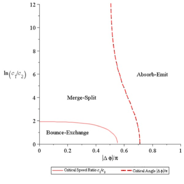
Figure 13. Types of $2$-soliton interactions for the Sasa-Satsuma equation

In the case of a double peak profile, the interaction is a bounce-exchange, i.e. where the fast and slow solitons first bounce and then exchange shapes and speeds at $t=x=0$. See Fig. 14.

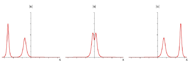
Figure 14. Sasa-Satsuma equation $2$-soliton interaction with $c_{1}/c_{2}=3$, $\phi_{1}-\phi_{2}=0.35\pi$

In the case of a single peak profile without side peaks, the interaction of the fast and slow solitons is a merge-split, i.e. where the solitons first merge together at $t=x=0$ and then split apart. See Fig. 15 and Fig. 16.

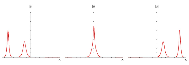
Figure 15. Sasa-Satsuma equation $2$-soliton interaction with $c_{1}/c_{2}=3$, $\phi_{1}-\phi_{2}=0.85\pi$

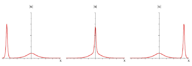
Figure 16. Sasa-Satsuma equation $2$-soliton interaction with $c_{1}/c_{2}=50$, $\phi_{1}-\phi_{2}=0.35\pi$

The case with side peaks is an absorb-emit interaction, i.e. where the slow soliton gradually is first absorbed by the front side of the fast soliton and is then emitted from the back side of the fast soliton. See Fig. 17 and Fig. 18.

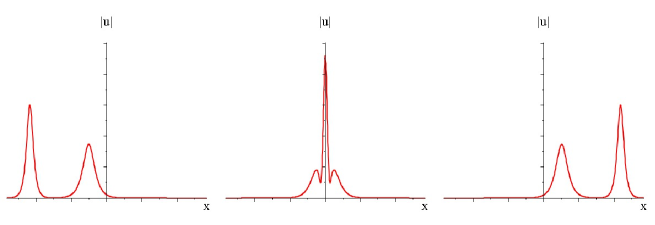
Figure 17. Sasa-Satsuma equation $2$-soliton interaction with $c_{1}/c_{2}=3$, $\phi_{1}-\phi_{2}=0.855\pi$

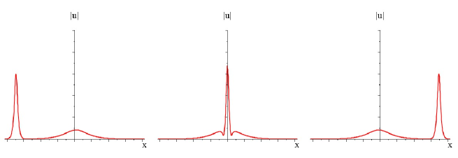
Figure 18. Sasa-Satsuma equation $2$-soliton interaction with $c_{1}/c_{2}=50$, $\phi_{1}-\phi_{2}=0.855\pi$

The special case of a saddle profile is shown in Fig. 19.

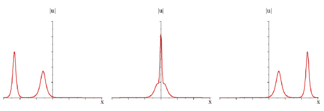
Figure 19. Sasa-Satsuma equation $2$-soliton interaction with $c_{1}/c_{2}=3$, $\phi_{1}-\phi_{2}=0.85032\pi$

5. Comparison of soliton collisions for the Hirota and Sasa-Satsuma equations

Up to a constant phase factor, the $2$-soliton solution for both the Hirota and Sasa-Satsuma equations reduces to the mKdV $2$-soliton solution when the relative phase angle $\Delta\phi$ between the fast and slow solitons in the collision is $0$ (same-orientation case) or $\pm\pi$ (opposite-orientation case).

In the Hirota $2$-soliton solution, the shift in positions of the fast and slow solitons is exactly the same as in the mKdV $2$-soliton solution, which depends only on the respective speeds $c_{1}$ and $c_{2}$ of the solitons. Moreover, in both the Hirota $2$-soliton solution and the mKdV $2$-soliton solution, there is no shift in the phase angles or orientations of the solitons.

In contrast, the position shifts of the fast and slow solitons in the Sasa-Satsuma $2$-soliton solution depend on their relative phase angle $\Delta\phi$ in addition to their speeds $c_{1}$ and $c_{2}$. See Fig. 20. More remarkable is that the collision changes the sign of the relative phase angle.

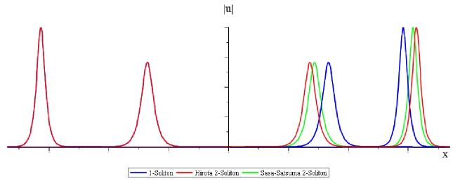
Figure 20. Sasa-Satsuma and Hirota $2$-soliton interactions with $c_{1}/c_{2}=2$, $\phi_{1}-\phi_{2}=0.5\pi$

Both the Sasa-Satsuma and Hirota $2$-soliton solutions describe three different types of collisions, which are separated by a critical speed ratio and a critical phase angle shown in Fig. 13 and Fig. 12. Interestingly, for collisions in the Sasa-Satsuma case, the angle $|\Delta\phi|\approx 0.55\pi$ at which the critical speed ratio $r_{+}$ approaches the limit ratio of $1$ is strictly less than the critical phase angle $|\Delta\phi|\approx 0.712\pi$ when $c_{1}/c_{2}$ approaches the same limit ratio of $1$, whereas these angles are both equal to $\pi$ for collisions in the Hirota case.

6. Concluding remarks

Our work in this paper studying the interaction properties of complex mKdV solitons can be extended in at least three interesting directions.

First, the Hirota equation (3.1) and the Sasa-Satsuma equation (4.1) are gauge-equivalent to a third order NLS equation [15]

$$q_{\tilde{t}}\pm i\sqrt{\frac{v}{2}}(3q_{\tilde{x}\tilde{x}}+|q|^{2}q)+\alpha|q|^{2}q_{\tilde{x}}+\beta|q||q|_{\tilde{x}}q+q_{\tilde{x}\tilde{x}\tilde{x}}=0$$ (6.1)

under the Galilean-phase transformation

$$u(t,x)=q(\tilde{t},\tilde{x})\exp\left(\pm i\sqrt{\frac{v}{2}}(\tilde{x}-v\tilde{t})\right)$$ (6.2)

where $v>0$ is a speed parameter, with $\alpha=24$, $\beta=0$ in the Hirota case and $\alpha=\beta=12$ in the Sasa-Satsuma case. Our main results (cf. Sec. 5) concerning the properties of collisions of solitary waves for the Hirota and Sasa-Satsuma equations will thus directly carry over to solitary waves of the form

$$q(\tilde{t},\tilde{x})=\frac{\sqrt{c}}{2}\exp\left(i\phi+i\omega\tilde{t}\right){\rm sech}\left(\sqrt{c}(\tilde{x}-\tilde{c}\tilde{t})\right)$$ (6.3)

with

$$\omega=\pm\sqrt{v/2}(c+v/2),\qquad\tilde{c}=c+3v/2>0$$ (6.4)

for the corresponding cases of the NLS equation (6.1). In particular, such solitary waves will exhibit three distinct types of collisions, which are separated by a critical speed ratio and a critical phase angle in terms of the speeds $\tilde{c}_{1}$, $\tilde{c}_{2}$, the phases $\phi_{1}$, $\phi_{2}$, and the frequencies $\omega_{1}$, $\omega_{2}$ of the solitary waves in the collision. For all collisions, the waves undergo position shifts in both the Hirota and Sasa-Satsuma cases, as well as phase shifts in the Sasa-Satsuma case, such that the shifts depend only on the parameters $c_{1}$, $c_{2}$, and $\phi_{1}-\phi_{2}$.

Second, as indicated by the correspondence (6.2), the Hirota and Sasa-Satsuma equations each admit more general solitary wave solutions given by the form

$$u(t,x)=\exp(i\psi(t))f(x-ct)$$ (6.5)

where

$$\psi(t)=\omega t+\phi$$ (6.6)

is a time-varying phase, with constant parameters $\omega,\phi$, and where $c>0$ is the wave speed. Collisions of such waves should display interesting interaction properties with new features beyond those with $\omega=0$ studied in Sec. 3 and Sec. 4.

Second, both the Hirota and Sasa-Satsuma equations have a natural multi-component generalization given by the two known types of $O(N)$-invariant integrable mKdV equations [17] for a $N$-component vector variable $\vec{u}$. In particular, under the identification between a $2$-component vector $\vec{u}=(u_{1},u_{2})$ and a complex scalar $u=u_{1}+iu_{2}$, the vector version of the Hirota equation (3.1) is given by

$$\vec{u}_{t}+24|\vec{u}|^{2}\vec{u}_{x}+\vec{u}_{xxx}=0$$ (6.7)

and the vector version of the Sasa-Satsuma equation (4.1) is given by

$$\vec{u}_{t}+12|\vec{u}|^{2}\vec{u}_{x}+12(\vec{u}\cdot\vec{u}_{x})\vec{u}+\vec{u}_{xxx}=0$$ (6.8)

For all $N\geq 2$, these two vector equations are integrable and admit vector solitary wave solutions of the form

$$\vec{u}(t,x)=f(x-ct)\hat{\psi}$$ (6.9)

with wave speed $c>0$, where $\hat{\psi}$ is an arbitrary constant unit vector and $f$ is the sech solitary wave profile for the real scalar mKdV equation (2.1). In forthcoming work, we plan to generalize the results in Sec. 3 and Sec. 4 to study the interaction properties of collisions of vector solitons of both equations (6.7) and (6.8) for $N>2$, where the collision involves a fast soliton with vector orientation $\hat{\psi}_{1}$ and speed $c_{1}$ overtaking a slow soliton with vector orientation $\hat{\psi}_{2}$ and speed $c_{2}$.

Appendix A

The $2$-soliton solution of the Sasa-Satsuma equation (4.1) can be derived most easily by a computational-ansatz version of the Hirota method [16] as follows. We first use the standard rational transformation

$$u=G/F$$ (A.1)

with $F$ real and $G$ complex. This transformation converts the Sasa-Satsuma equation into the equivalent rational form

$$0=\frac{1}{F^{2}}\big{(}D_{t}(G,F)+D_{x}^{3}(G,F)\big{)}+\frac{1}{F^{3}}\big{(}6GD_{x}(\bar{G},G)\big{)}+\frac{1}{F^{4}}\big{(}24|G|^{2}-3D_{x}^{2}(F,F))D_{x}(G,F)\big{)}$$ (A.2)

as written in terms of Hirota’s bilinear $D$ operator given by

$$D(a,b)=bDa-aDb$$ (A.3)

$$D^{2}(a,b)=bD^{2}a+aD^{2}b-2(Da)Db$$ (A.4)

$$D^{3}(a,b)=bD^{3}a-3(Db)D^{2}a+3(Da)D^{2}b-aD^{3}b$$ (A.5)

Through the introduction of an auxiliary variable $H$, there is a natural splitting of equation (A.2) into a bilinear system of equations

$$D_{x}^{2}(F,F)=8G\bar{G},\quad D_{t}(G,F)+D_{x}^{3}(G,F)=iHG,\quad iFH=6D_{x}(G,\bar{G})$$ (A.6)

for the real variables $F,H$ and the complex variable $G$.

We now observe that the $1$-soliton solution of the bilinear system (A.6) is given by the simple exponential polynomials

$$G=A\exp(\theta),\quad F=1+B\exp(2\theta),\quad H=0$$ (A.7)

with

$$\theta=kx-\omega t,\quad\omega=k^{3},$$ (A.8)

where $A$ and $B$ are respectively complex and real parameters satisfying the algebraic relation

$$|A|^{2}=k^{2}B$$ (A.9)

In particular, if we write $A=|A|\exp(i\phi)$ by a polar decomposition and express $B=(|A|/k)^{2}$, this yields

$$G=k\exp(k\xi),\quad F=1+\exp(2k\xi)$$ (A.10)

in terms of the moving coordinate

$$\xi=x-k^{2}t-x_{0}$$ (A.11)

which is centered at the initial position

$$x_{0}=\ln(k/|A|)/k$$ (A.12)

Then the rational exponential solution obtained from expressions (A.1) and (A.10) matches the solitary wave solution (4.2)–(4.3) having speed $c=k^{2}>0$ and center of momentum $\chi(t)=k^{2}t+x_{0}$.

To obtain the $2$-soliton solution of the bilinear system (A.6), we use the ansatz

$$G= A_{1}\exp(\theta_{1})+A_{2}\exp(\theta_{2})+C_{1}\exp(\theta_{1}+2\theta_{2})+C_{2}\exp(\theta_{2}+2\theta_{1})$$ (A.13)

$$F= 1+B_{1}\exp(2\theta_{1})+B_{2}\exp(2\theta_{2})+I\exp(\theta_{1}+\theta_{2})+J\exp(2\theta_{1}+2\theta_{2})$$ (A.14)

and

$$H=K\exp(\theta_{1}+\theta_{2})$$ (A.15)

with

$$\theta_{1}=k_{1}x-\omega_{1}t,\quad\theta_{2}=k_{2}x-\omega_{2}t,$$ (A.16)

where $B_{1},B_{2},I,J,K$ are real parameters, and $A_{1},A_{2},C_{1},C_{2}$ are complex parameters. In this ansatz, the form (A.13)–(A.14) for the variables $G,F$ is motivated by the rational exponential form of the mKdV $2$-soliton (2.13), while the form (A.15) for the auxiliary variable $H$ comes from balancing the highest-power terms in the third equation in the bilinear system (A.6). Substitution of $G,F,H$ into the system (A.6) leads to three equations, which are each a polynomial in the exponentials $\exp(\theta_{1})$ and $\exp(\theta_{2})$. The coefficients of these polynomials directly yield an overdetermined bilinear system of algebraic equations that can be solved for the parameters $B_{1},B_{2},I,J,K,C_{1},C_{2}$ in terms of the pair of complex parameters $A_{1},A_{2}$. This gives us the result (obtained by a Maple calculation)

$$\omega_{1}=k_{1}^{3},\quad\omega_{2}=k_{2}^{3},\quad\theta_{1}=k_{1}(x-k_{1}^{2}t),\quad\theta_{2}=k_{2}(x-k_{2}^{2}t),$$ (A.17)

$$B_{1}=\frac{|A_{1}|^{2}}{k_{1}^{2}},\quad B_{2}=\frac{|A_{2}|^{2}}{k_{2}^{2}},$$ (A.18)

$$C_{1}=\frac{(k_{1}-k_{2})(k_{1}A_{1}\bar{A}_{2}-k_{2}A_{2}\bar{A}_{1})A_{2}}{k_{2}^{2}(k_{1}+k_{2})^{2}},\quad C_{2}=\frac{(k_{1}-k_{2})(k_{1}A_{1}\bar{A}_{2}-k_{2}A_{2}\bar{A}_{1})A_{1}}{k_{1}^{2}(k_{1}+k_{2})^{2}},$$ (A.19)

$$I=4\frac{A_{1}\bar{A}_{2}+A_{2}\bar{A}_{1}}{(k_{1}+k_{2})^{2}},\quad J=\frac{(k_{1}-k_{2})^{2}(k_{1}A_{2}\bar{A}_{1}-k_{2}A_{1}\bar{A}_{2})(k_{1}A_{1}\bar{A}_{2}-k_{2}A_{2}\bar{A}_{1})}{k_{1}^{2}k_{2}^{2}(k_{1}+k_{2})^{4}},$$ (A.20)

$$K=6(k_{1}-k_{2})(iA_{2}\bar{A}_{1}-iA_{1}\bar{A}_{2})$$ (A.21)

Note this solution (A.13)–(A.20) contains a pair of arbitrary phases and positions corresponding to the parameters

$$A_{1}=|A_{1}|\exp(i\psi_{1}),\quad A_{2}=|A_{2}|\exp(i\psi_{2})$$ (A.22)

We now simplify the form of the $2$-soliton solution (A.13)–(A.14) and (A.17)–(A.20) by the following steps. First we observe

$$k_{2}^{2}C_{1}/A_{2}=k_{1}^{2}C_{2}/A_{1}=|A_{1}||A_{2}|C$$ (A.23)

$$J=(C_{1}/A_{2})(\bar{C}_{2}/\bar{A}_{1})=(|A_{1}||A_{2}||C|)^{2}/(k_{1}k_{2})^{2}$$ (A.24)

where

$$C=\frac{(k_{1}-k_{2})}{(k_{1}+k_{2})^{2}}(k_{1}\exp(i\Delta\psi)-k_{2}\exp(-i\Delta\psi)),\quad\Delta\psi=\psi_{1}-\psi_{2}$$ (A.25)

Next we introduce the moving coordinates

$$\xi_{1}=x-k_{1}^{2}t-x_{1},\quad\xi_{2}=x-k_{2}^{2}t-x_{2}$$ (A.26)

centered at initial positions

$$x_{1}=\ln\big{(}k_{1}/(|A_{1}|\sqrt{|C|})\big{)}/k_{1},\quad x_{2}=\ln\big{(}k_{2}/(|A_{2}|\sqrt{|C|})\big{)}/k_{2}$$ (A.27)

which are determined in terms of $|A_{1}|$ and $|A_{2}|$. Then the exponential polynomials (A.13) for $G$ and (A.13) for $F$ are given by

$$G= \frac{1}{\sqrt{|C|}}\Big{(}k_{1}\exp(\theta_{1})\big{(}\exp(i\psi_{1})+\exp(i(\psi_{2}+\psi))\exp(2\theta_{2})\big{)}$$

$$\qquad k_{2}\exp(\theta_{2})\big{(}\exp(i\psi_{2})+\exp(i(\psi_{1}+\psi))\exp(2\theta_{1})\big{)}\Big{)}$$ (A.28)

$$F= 1+\exp(2\theta_{1}+2\theta_{2})+\frac{1}{|C|}\Big{(}\exp(2\theta_{1})+\exp(2\theta_{2})$$

$$\qquad+4k_{1}k_{2}(k_{1}+k_{2})^{-2}\big{(}\exp(i\Delta\psi)+\exp(-i\Delta\psi)\big{)}\exp(\theta_{1}+\theta_{2})\Big{)}$$ (A.29)

in terms of

$$\theta_{1}=k_{1}\xi_{1},\quad\theta_{2}=k_{2}\xi_{2}$$ (A.30)

and

$$\exp(i2\psi)=C/\bar{C}=\frac{k_{1}\exp(i\Delta\psi)-k_{2}\exp(-i\Delta\psi)}{k_{1}\exp(-i\Delta\psi)-k_{2}\exp(i\Delta\psi)}$$ (A.31)

These expressions (A.28) and (A.29) match the form of the colliding solitary wave solution (4.4)–(4.6) if we write

$$\psi=\phi_{2}-\phi_{1},\quad\psi_{1}=\phi_{1},\quad\psi_{2}=\phi_{1}-\Delta\psi$$ (A.32)

and use relations (A.31) and (A.25) to express

$$\exp(i\Delta\psi)=\frac{1}{\gamma}\big{(}k_{1}\exp(i\psi)+k_{2}\exp(-i\psi)\big{)}=\exp(-i(\nu_{1}-\psi))=\exp(-i(\nu_{2}+\psi))$$ (A.33)

and

$$|C|=\frac{k_{1}-k_{2}}{(k_{1}+k_{2})^{2}}\frac{k_{1}^{2}-k_{2}^{2}}{\gamma}=\frac{1}{\gamma\rho^{2}}$$ (A.34)

where

$$\gamma=\sqrt{k_{1}^{2}+k_{2}^{2}+2k_{1}k_{2}\cos(2\psi)},\quad\rho=\frac{\sqrt{k_{1}+k_{2}}}{k_{1}-k_{2}}$$ (A.35)

References

- [1] M.J. Ablowitz and P.A. Clarkson, Solitons, Nonlinear Evolution Equations and Inverse Scattering, London Math. Soc. Lecture Note Series 149 (Cambridge University Press) 1991.
- [2] P.D. Lax, Commun. Pure Appl. Math. 21 (1968) 467–490.
- [3] R.J. LeVeque, SIAM J. Appl. Math. 47 (1987) 254–262.
- [4] N. Benes, A. Kasman, K. Young, J. Nonlin. Sci. 16 (2006) 179–200.
- [5] G.B. Whitham, Linear and Nonlinear Waves, (John Wiley& Sons) 1974.
- [6] J.H.B. Nijhof and G.H.M. Roelofs, J. Phys. A: Math. Gen. 25 (1992) 2403–2416.
- [7] S.Y. Sakovich, J. Phys. Soc. Jpn. 66 (1997) 2527–2529.
- [8] S. Anco, M. Mohiuddin, T. Wolf, in preparation (2011).
- [9] R. Hirota, J. Math. Phys. 14 (1973) 805–809.
- [10] N. Sasa and J. Satsuma, J. Phys. Soc. Jpn. 60 (1991) 409–417.
- [11] R.M. Miura, C.S. Gardner, M.S. Kruskal, J. Math. Phys. 9 (1968) 1204–1209.
- [12] R. Hirota, J. Phys. Soc. Jpn. 22 (1972) 1456–1458.
- [13] M. Wadati and M. Toda, J. Phys. Soc. Jpn. 34 (1972) 1289–1296.
- [14] M. Wadati and M. Toda, J. Phys. Soc. Jpn. 32 (1972) 1403–1411.
- [15] C. Gilson, J. Hietarinta, J. Nimmo, Y. Ohta, Phys. Rev. E 68 (2003) 016614 (10 pages).
- [16] R. Hirota, The Direct Method in Soliton Theory, Cambridge Tracts in Math. 155 (Cambridge University Press) 1992.
- [17] V.V. Sokolov and T. Wolf, J. Phys. A: Math. Gen. 34 (2001), 11139–11148.