Test-State Approach to the Quantum Search Problem

Abstract

The search for “a quantum needle in a quantum haystack” is a metaphor for the problem of finding out which one of a permissible set of unitary mappings—the oracles—is implemented by a given black box. Grover’s algorithm solves this problem with quadratic speed-up as compared with the analogous search for “a classical needle in a classical haystack.” Since the outcome of Grover’s algorithm is probabilistic—it gives the correct answer with high probability, not with certainty—the answer requires verification. For this purpose we introduce specific test states, one for each oracle. These test states can also be used to realize “a classical search for the quantum needle” which is deterministic—it always gives a definite answer after a finite number of steps—and faster by a factor of $3.41$ than the purely classical search. Since the test-state search and Grover’s algorithm look for the same quantum needle, the average number of oracle queries of the test-state search is the classical benchmark for Grover’s algorithm.

I Introduction

In recent decades, the quantum theory found another practical use in the field of quantum information processing: Quantum computation QC1 ; QC2 ; QC3 and quantum information theory QI1 ; QI2 are extensively researched by several scientific communities. On one hand, the superposition principle of quantum mechanics speeds up the computation for important classes of computational problems. On the other hand, entanglement assists us in sending information from one place to another in a secure way. Both branches—quantum computation and quantum information theory—are interlinked and are growing rapidly.

“Searching an item in a given database” is a well-known computational problem which has been studied with different conditions in both classical CC and quantum GA contexts. When an unsorted database stored in the memory of a classical computer (CC) is given, then the average number of iterations required by the CC to complete this classical search grows linearly with the total number of items present in the database. But, if the items are already present in an order in the memory, then the average number of iterations scales up logarithmically with respect to the total number of items.

Grover introduced a quantum search algorithm GA for an analogous “quantum search problem:” A quantum computer (QC) searches a particular ket out of a set of kets from the computational basis. Or, more precisely, the quantum search finds which one of a set of unitary mappings—the oracles—is implemented by a black box. One can tackle this problem like its classical analog by testing for each oracle one by one in a sequence till the match is found. Alternatively, we can exploit the superposition principle and address all the oracles simultaneously, with Grover’s search algorithm (GA). This gives a quadratic speedup to GA in comparison with the classical search.

But the answer returned by GA is the correct one with a high probability only, not with certainty. It is, therefore, necessary to verify the answer. This verification is done with the aid of the test states that we introduce here, one test state for each oracle.

The test states can also be used for a classical-type search of the quantum data set (that is, the set of oracles). Such a test-state search is deterministic—it will give the correct answer after a finite number of queries—and the average number of queries is proportional to the number of permissible oracles, but fewer by a factor of $3.41$ than the average number of queries for the corresponding classical search of an unstructured classical database.

A single iteration of the test-state approach is a three-step process. First, we prepare a test state, which is a certain superposition of all the kets of the set under search. Second, we pass it through the oracle—the very same oracle that is employed by GA. Finally, we retrieve the information by a measurement on the processed test state. As is the case in the classical search, this measurement says “yes” or “no” if the test state matches the oracle or not. In marked contrast to the classical search problem, however, there are different “no” answers depending on the actual oracle, and the measurement extract the available information. The choice of test state for the next round is then guided by this information, and this guidance leads to a substantial reduction of the average number of trials needed before successful termination of the search.

The structure of this article is as follows. Section II comprises of the definitions and the algorithms for the search problem in both classical and quantum contexts. In Sec. III, a comprehensive description of the test-state approach to the quantum search problem is provided. GA with test-state verification is then discussed in Sec. IV, and Sec. V deals with alternative test-state search strategies. In Sec. VI, we describe the quantum circuit for the construction of the test state and for realizing the measurements. We conclude with a summary and discussion in Sec. VII, and two appendixes contain additional material.

II Search problem

Suppose someone gives us a list of one hundred names of different animals on a piece of paper, and ask where “Lion” appears on this list. If “Lion” appears exactly once on the list, and the list is not ordered in any obvious way, then we have to go through about fifty names on average before we find “Lion.” For a search of this kind, neither a CC nor a QC can directly helps us, because the data (names) are given on a piece of paper.

In order to use a CC or a QC for this kind of database search, first we have to convert the data into an accessible format. For example, in case of a CC for such a search, first we have to load the data (the given list) into the memory of a CC. However, we can find the name Lion in the process of converting the list of names into an electronic format (in terms of strings of bits) and storing them in the memory. So, neither a CC nor a QC is very helpful for a search of this kind. In other words, a CC (QC) is helpful for a database search only when the database is given in an electronic format (quantum format).

Furthermore, a QC also cannot search a classical database without a “quantum addressing scheme” QCQI where the classical database is converted into a quantum format (in terms of quantum kets). So, the process of searching a marked string of bits with a CC in a classical database which is stored in the memory of a computer is called as classical search. Similarly, quantum search is a process where a QC searches a marked quantum state (or, rather, a particular unitary operation) out of a set of quantum states (or, rather, a set of unitary operations). Classical and quantum searches are analogous but not the same, their detailed description is given in the following.

II.1 Classical search

Suppose we have an unsorted database as a set

$$\mathcal{S}^{N}_{C}\equiv\{0,\cdots,j,\cdots,N-1\}$$ (1)

of a total of $N$ items stored electronically in the memory of a CC. Each item is labeled by an index from 0 to $N-1$ and further represented by a $n$-bit string in binary representation. For convenience, we shall confine our attention to the case $N=2^{n}$ ($0\equiv 00\cdots 0$, $N-1\equiv 11\cdots 1$), but the following algorithms and the test-state approach can be implemented for an arbitrary value of $N$.

Throughout the article we shall consider only the case of a single matching item. The task of the search problem is to recover the corresponding index ($n$-bit string) to the marked item at the end of computation.

The method employed by a CC to solve the search problem is by checking every element of $\mathcal{S}^{N}_{C}$ one by one in a sequence till a match is found CC . A single iteration of this classical algorithm is a three-step process given as follows. Step 1: The CC picks a $n$-bit string at random from the set $\mathcal{S}^{N}_{C}$ as an input. Step 2: The CC checks whether or not this string matches with our query. Step 3: It produces an answer to the question in terms of “yes” or “no.” If the answer is “yes,” then the CC stops the computation and produces the string as the result, and the corresponding item will be the matching item. If the answer turns out to be “no,” then the CC picks another string at random from the set $\mathcal{S}^{N}_{C}$ as an input, with items tested earlier excluded, and asks the same question. If the answer is again “no,” then the CC repeats the above procedure until it hits the matching item. One of the main points in this classical algorithm is, “Every time the CC picks at random only one $n$-bit string, and its current guess does not depend on previous guesses” other than excluding them. In this way, a CC needs, on average, as many as

$$\mathit{G}_{C}(N)=\frac{N+1}{2}-\frac{1}{N}$$ (2)

queries of the database before it finds the matching item. This is an immediate consequence of the recurrence relation

$$\mathit{G}_{C}(N+1)=1+\frac{N}{N+1}G_{C}(N)\quad\mbox{for}\enskip N>1$$ (3)

that commences with $G_{C}(1)=0$.

Since $\mathit{G}_{C}(N)\propto N$ for $N\gg 1$, this classical search algorithm is linear in the number of candidate items. If, rather than being unstructured, the data were sorted beforehand, then the problem could be completed by a binary search in approximately $\log_{2}N$ iterations CC .

II.2 Quantum search

In this section, an analogous quantum search problem to the classical one and a brief description of GA GA is provided. Throughout the text we represent the single-qubit Pauli vector operator $\vec{\sigma}$ by $\left(X,Y,Z\right)$ and the identity operator by $I$.

In the step from classical to quantum, bits are replaced by qubits. So, for each index ($n$-bit string) $j$ of $\mathcal{S}^{N}_{C}$ defined by Eq. (1) there exist a $n$-qubit quantum ket $|j\rangle$, the so-called index ket. There is then a unitary operation $\mathcal{O}^{j}$—the $j$th oracle—which gives a conditional phase shift of $\pi$ to the index ket $|j\rangle$ only,

$$\mathcal{O}^{j}\equiv{(-\mathcal{I})}^{|j\rangle\langle j|}=\mathcal{I}-2|j\rangle\langle j|\,,$$ (4)

where $\mathcal{I}=I^{\otimes n}$ is the identity operator in the $N$-dimensional Hilbert space.

One can define an analogous quantum search problem to the classical search problem of Sec. II.1 in the following way: Suppose someone gives us a quantum black box, which is implementing one of the $N$ different oracles, and asks us to find out which of the oracles is the case without actually opening the box and looking inside. Clearly, we are not using QC to search a marked item in a classical database, but we are searching the index ket corresponding to the given oracle. The question of how many queries of the database are now needed, reads “How many times must one use the quantum black box to find out the correct result?”

The most efficient way of finding out which oracle is the actual one is GA optGA . GA begins by applying the Hadamard gate

$$H=(X+Z)/\sqrt{2}$$ (5)

to each qubit, after initially preparing the state with index ket $|0\rangle\equiv|0\rangle^{\otimes n}$. The operation $H^{\otimes n}$ creates a superposition of all the index kets of $\mathcal{S}^{N}_{Q}$ with equal amplitude $1/\sqrt{N}$. The next step is an application of the Grover iteration operator $\mathcal{G}$, geometrically it is a rotation composed of two reflection operations as $\mathcal{G}=\mathcal{D}\mathcal{O}$. The operator $\mathcal{O}$ is the same quantum oracle (black box) defined by Eq. (4), whose unknown index we have to find. The diffusion operator $\mathcal{D}$ gives an inversion about the average GA ,

$$\mathcal{D}=-H^{\otimes n}\bigl{(}\mathcal{I}-2|0\rangle\langle 0|\bigr{)}H^{\otimes n};$$ (6)

its central piece is the $0$th oracle $\mathcal{O}^{0}$.

GA is probabilistic in nature in the sense that, after applying $\mathcal{G}$ several times, the probability of the privileged index ket becomes significantly higher than the probabilities of the other index kets. Finally, we read out the output by performing projective measurements on each qubit, and so find one of the index kets. After $k$ applications of $\mathcal{G}$, we have GA

$$p^{(N)}_{k}=\sin\bigl{(}(2k+1)\theta_{N}\bigr{)}^{2}\quad\mbox{with}\enskip\sin\theta_{N}=1/\sqrt{N}$$ (7)

for the probability that the oracle associated with the final output state is the one which the black box is executing. Upon optimizing $k$, GA solves the quantum search problem by using the black box only

$$\mathit{G}_{Q}(N)=0.69\sqrt{N}$$ (8)

times when ${N\gg 1}$; see Sec. IV below. The quadratic speedup of $\mathit{G}_{Q}(N)\propto\sqrt{N}$ versus $\mathit{G}_{C}(N)\propto{N}$ is owed to the computational power of quantum physics; specifically, the superposition principle is at work. We emphasize that the outcome of GA is not guaranteed to be the correct answer; it can be incorrect with a probability that is very small but definitely nonzero.

In passing, we note the following. A general treatment of GA for multiple targets and for an arbitrary value of $N$ is given in Ref. multGA . Moreover, GA is a special case of the quantum amplitude amplification QAA . In addition, one can get rid of the probabilistic nature of GA if one has the option of changing the structure of the diffusion operator $\mathcal{D}$ and the oracle $\mathcal{O}$ extGA . When one is only allowed to use the given black box, namely the oracles of Eq. (4), but not to look inside and change the setting, then GA remains probabilistic in nature.

So, one needs a confirmation step to be sure of the result obtained by GA. A single iteration of the test-state search introduced in the next section acts as a confirmation step for GA, where the verification matter is discussed after Eqs. (15). Details of GA with test-state verification are given in Sec. IV.

III Test-state search

In this section, we introduce the test-state approach to the quantum search problem described in Sec. II.2—where one has to identify the actual oracle which is implemented by the given black box. The features of both classical and quantum approaches are embodied in this approach. A single iteration in the test-state approach can be summarized in the following three steps.

Step 1: We pick an index ket $|j\rangle$ and prepare the corresponding test state. Step 2: We pass the test state through the given quantum black box which is executing one of the oracles of Eq. (4). Step 3: We extract the information with the help of a particular probability-operator measurement (POM) POVM1 ; POVM2 . Here, a “single iteration” comprises of these three steps, which are similar to the classical search algorithm of Sec. II.1. The result of the POM gives an answer to the same question—whether or not the black box is executing the oracle $\mathcal{O}^{j}$—in terms of “yes” or “no.” The answer “yes” tells us that the black box is executing the corresponding oracle to the index ket we picked, and we terminate the search.

Even if the answer is “no,” the result of the POM gives us some information about the actual oracle. This information facilitates an educated guess and a judicious choice of the test state for the next iteration.

The correct result is obtained after a finite number of iterations. In other words, the test-state search is deterministic, rather than probabilistic. And, the systematic educated guessing makes the test-state search more efficient than a truly classical search, in which all test states would be chosen at random: For $N\gg 1$, the test-state search needs fewer guesses by a factor of $3.41$.

III.1 A single iteration in the test-state search

In this section, we construct the test states for verification of the outcome of GA and discuss the three steps of one iteration round in the test-state approach to determining the actual oracle of the quantum search problem. The narrative follows the steps in sequence.

Step 1—Preparing the test state: We pick an index ket $|j\rangle$ from the set

$$S^{N}_{Q}=\bigl{\{}|0\rangle,\dots,|j\rangle,\dots,|N-1\rangle\bigr{\}}$$ (9)

of all index kets. For the very first round of iteration, the choice of $|j\rangle$ is random, but for all subsequent rounds the choice is dictated by the result of the measurement in Step 3, as discussed in Sec. III.2.

Then we prepare the corresponding test state $|t_{j}\rangle$ which is of the form

$$|t_{j}\rangle=a|j\rangle+b\sum_{l(\neq j)}|l\rangle\,,$$ (10)

where $a$ is the amplitude of the privileged index ket $|j\rangle$ and $b$ is the common amplitude of all other index kets. Both $a$ and $b$ are functions of $N$; it suffices to consider only real positive values for $a$ and $b$, but this is a restriction of convenience, not of necessity.

In Sec. VI.1, we present a quantum circuit for constructing the test state $|t_{0}\rangle$. The test state $|t_{0}\rangle$ can be transformed into any other test state $|t_{j}\rangle$ by applying the $X$ operations on the relevant qubits. In other words, each $|t_{j}\rangle$ is equivalent to $|t_{0}\rangle$ up to some single-qubit operations.

Step 2—Processing the test state: We pass the test state $|t_{j}\rangle$ through the given quantum black box. We recall that the black box is implementing one of the $N$ different oracles of Eq. (4), but we do not know which oracle is the case. If the black box is implementing the $j$th oracle, then the resultant state is

$$\mathcal{O}^{j}|t_{j}\rangle=|t_{j}^{j}\rangle=-a|j\rangle+b\sum_{l(\neq j)}|l\rangle.$$ (11)

If the black box is not implementing the $j$th oracle, but some other one, the $k$th oracle, say, then the resultant state is

$$k\neq j\,:\quad\mathcal{O}^{k}|t_{j}\rangle=|t_{j}^{k}\rangle=a|j\rangle-b|k\rangle+b\sum_{l(\neq j,k)}|l\rangle.$$ (12)

Result $|t_{j}^{j}\rangle$ says “yes, it is the $j$th oracle” whereas each $|t_{j}^{k}\rangle$ with $k\neq j$ says “no, it is not the $j$th oracle,” and we note that there is one “yes” but $N-1$ different “no”s.

We define the “no” set $\mathcal{C}_{j}^{N}$ to index ket $|j\rangle$ as the collection of all $N-1$ “no” states of Eq. (12),

$$\mathcal{C}_{j}^{N}=\bigl{\{}|t_{j}^{0}\rangle,\cdots,|t_{j}^{j-1}\rangle,|t_{j}^{j+1}\rangle,\cdots,|t_{j}^{N-1}\rangle\bigr{\}}.$$ (13)

In order to be able to distinguish the “yes” ket $|t_{j}^{j}\rangle$ from the “no” kets in $\mathcal{C}_{j}^{N}$, we demand that

$$\langle t_{j}^{k}\arrowvert t_{j}^{j}\rangle=0\quad\mbox{for $k\neq j$},$$ (14)

so that the “yes” ket is orthogonal to all “no” kets. Together with the normalization of the test-state ket $|t_{j}^{j}\rangle$, this gives

$$a = \sqrt{(N-3)/(2N-4)},$$

$$b = \sqrt{1/(2N-4)},$$ (15)

for the amplitudes in Eq. (10).

The use of the test states for the verification of the outcome of GA, is quite obvious: After GA identifies the $j$th oracle, we prepare the $j$th test state $|t_{j}\rangle$ and let the oracle act on it. Then we perform a measurement that determines whether the resulting ket is proportional to the “yes” ket $|t_{j}^{j}\rangle$ or resides in the orthogonal subspace spanned by the ${N-1}$ “no” kets. If we find the “yes” ket, the search is over; otherwise, we have to execute GA another time. An alternative confirmation step for GA, where one has to use the black box at most two times, is described in Appendix A.

As Eqs. (15) show, there are test states for $N>2$, but none for $N=2$. This is as it should be. For, the two $N=2$ oracles $\mathcal{O}^{0}=|1\rangle\langle 1|-|0\rangle\langle 0|$ and $\mathcal{O}^{1}=|0\rangle\langle 0|-|1\rangle\langle 1|$ are simply indistinguishable; they do not tell the index kets $|0\rangle$ and $|1\rangle$ apart.

Turning our attention to the “no” kets, we observe that they are the edges of a $(N-1)$-dimensional pyramid,

$$k\neq j,\ l\neq j\,:\quad\langle t_{j}^{k}\arrowvert t_{j}^{l}\rangle=\lambda+(1-\lambda)\delta_{kl}$$ (16)

with $\lambda=(N-4)/(N-2)$. In the terminology of Ref. pyramid3 , the pyramid is acute ($\lambda>0$) for $N>4$, orthogonal ($\lambda=0$) for $N=4$, and flat ($\lambda=-1/(N-2)$) for $N=3$.

The case $N=4$ is particular: We have $a=b=1/2$ and all four test states are identical. The “no” states for one index ket are pairwise orthogonal; they are “yes” states for the other index kets. As a consequence, testing the oracle once with the one common test state will reveal its identity.

This observation is sometimes stated as “GA needs to query the oracle only once for $N=4$.” Indeed, we have $p^{(4)}_{1}=1$ in Eq. (7). This peculiarity of GA comes about because the common ${N=4}$ test state is also the ${N=4}$ initial state of GA, and the ${N=4}$ version of the diffusion operator $\mathcal{D}$ of Eq. (6) maps the SRM kets of Eq. (20) below onto the computational basis, in which the outcome of GA is obtained.

Step 3—Measuring the result: When measuring the state that results from applying the black-box oracle to the $j$th test state $|t_{j}\rangle$, we not only need to distinguish between “yes” and “no” but also want to acquire information about which of the “no”s is the case, so that we can make a judicious choice for the next test state. Thanks to the pyramidal structure of the “no” kets, the POM that maximizes our odds of guessing right is the so-called square-root measurement (SRM) SRM ; pyramid3 .

For $N=3$, there is no useful POM of this kind because the two “no” states are the same, as is exemplified by $|t_{0}^{1}\rangle=-|t_{0}^{2}\rangle$. For $N>3$, the SRM

$$\sum_{k=0}^{N-1}\Pi_{j}^{k}=\mathcal{I}$$ (17)

has the rank-1 outcomes $\Pi_{j}^{k}=|T_{j}^{k}\rangle\langle T_{j}^{k}|$ with

$$|T_{j}^{k}\rangle = {\left(\sum_{l=0}^{N-1}|t_{j}^{l}\rangle\langle t_{j}^{l}|\right)}^{-1/2}|t_{j}^{k}\rangle$$ (20)

$$= \left\{\begin{array}[]{l}\rule{0.0pt}{12.91663pt}|t_{j}^{j}\rangle\quad\mbox{for}\enskip k=j\\[4.30554pt] \displaystyle b|j\rangle-x|k\rangle+y\sum_{l(\neq j,k)}|l\rangle\quad\mbox{for}\enskip k\neq j\end{array}\right.$$

where

$$y=\frac{1+a}{N-1},\quad x=1-y$$ (21)

and $a,b$ are the coefficients of Eqs. (10)–(12) and (15).

Since

$$\langle T_{j}^{k}|T_{j}^{l}\rangle=\delta_{kl},$$ (22)

the SRM is an orthogonal measurement, a standard von Neumann measurement, not a POM proper. Therefore, the SRM can be implemented by a unitary transformation followed by measuring the computational basis. One quantum circuit for such a unitary transformation is given in Sec. VI.2.

III.2 Conditional probabilities

The probability of getting the $l$th outcome if the processed $j$th test state is $|t_{j}^{k}\rangle$ is given by

$$\mathrm{prob}(t_{j}^{k}\to\Pi_{j}^{l})=\langle t_{j}^{k}|\Pi_{j}^{l}|t_{j}^{k}\rangle=\left|\langle T_{j}^{l}|t_{j}^{k}\rangle\right|^{2}.$$ (23)

It follows from Eqs. (11), (12), and (20) that there are three cases,

$$\mathrm{prob}(t_{j}^{k}\to\Pi_{j}^{l})=\left\{\begin{array}[]{l@{\ \mbox{for}\ }r}1&k=j,\ l=k\\ \alpha_{N-1}&k\neq j,\ l=k\\ \beta_{N-1}&k\neq j,\ l\neq k\end{array}\right.$$ (24)

where

$$\beta_{N-1} = \frac{1}{(N-1)^{2}}{\left(\sqrt{N-3}-\frac{\sqrt{2}}{\sqrt{N-2}}\right)}^{2},$$

$$\alpha_{N-1} = 1-(N-2)\beta_{N-1}$$ (25)

$$= \frac{1}{(N-1)^{2}}{\left(\sqrt{N-3}+\sqrt{2N-4}\right)}^{2},$$

with the subscript ${N-1}$ stating the number of different “no” outcomes.

The first case in Eq. (24) is the affirmative “yes, it is the $j$th oracle” answer that terminates the search. The second and third cases both say “no, it is not the $j$th oracle.” Thereby, the probability $\alpha_{N-1}$ of getting the $k$th outcome when the black box implements the $k$th oracle is larger than the probability $\beta_{N-1}$ for all other “no” outcomes. Upon finding the $l$th outcome, we will therefore guess that the black box contains the $l$th oracle and choose $|t_{l}\rangle$ as the next test state. The choice of SRM maximizes the probability that this educated guess is right.

After the first wrong guess $|j\rangle$, we exclude the index ket $|j\rangle$ from the list of candidates, and have the set

$$\mathcal{S}^{N-1}_{Q}=\bigl{\{}|0\rangle,\cdots,|j-1\rangle,|j+1\rangle,\cdots,|N-1\rangle\bigr{\}}$$ (26)

of the remaining $N-1$ index kets for the next round. Having found SRM outcome $\Pi_{j}^{l}$, we repeat the iteration described in Sec. III.1 on the set $\mathcal{S}^{N-1}_{Q}$ by taking the index ket $|l\rangle$ as the next educated guess, for which the “no” probabilities are $\alpha_{N-2}$ and $\beta_{N-2}$. If this guess is also wrong, then the $l$th index ket can be excluded as well, and we are left with $N-2$ candidates and a new educated guess for the next test state with “no” probabilities $\alpha_{N-3}$ and $\beta_{N-3}$. And so forth, until we either get the “yes” answer, or we are left with four candidates only, having excluded $N-4$ index kets successively. The common test state for $N=4$ will then surely give us the “yes” answer; in the present context, this is confirmed by $\alpha_{3}=1$ and $\beta_{3}=0$ in Eqs. (24) and (III.2).

In each round of iteration in the test-state search, we are using the black box once. Accordingly, the average number of oracle queries before a “yes” answer is obtained, is given by

$$\mathit{G}_{T}(N)=p^{(N)}_{1}+2p^{(N)}_{2}+3p^{(N)}_{3}+\dots+(N-3)p^{(N)}_{N-3}$$ (27)

where $p^{(N)}_{m}$ is the probability that the search terminates after the $m$th round. For $N>4$, these probabilities are

$$p^{(N)}_{1} = \frac{1}{N},$$

$$p^{(N)}_{2} = (1-p^{(N)}_{1})\alpha_{N-1}=\frac{N-1}{N}\alpha_{N-1},$$

$$p^{(N)}_{3} = (1-p^{(N)}_{1}-p^{(N)}_{2})\alpha_{N-2}$$ (28)

$$= \frac{N-1}{N}(1-\alpha_{N-1})\alpha_{N-2},$$

$$\vdots$$

$$p^{(N)}_{N-4} = (1-p^{(N)}_{1}-p^{(N)}_{2}-\cdots-p^{(N)}_{N-5})\alpha_{5}$$

$$= \frac{N-1}{N}(1-\alpha_{N-1})\cdots(1-\alpha_{6})\alpha_{5}$$

$$p^{(N)}_{N-3} = 1-p^{(N)}_{1}-p^{(N)}_{2}-\cdots-p^{(N)}_{N-4}$$

$$= \frac{N-1}{N}(1-\alpha_{N-1})\cdots(1-\alpha_{6})(1-\alpha_{5}).$$

Without the educated guesses provided by the SRM, one would have to resort to choosing the test state for the next iteration at random, just as one does in a purely classical search, which amounts to the replacement $\alpha_{L}\to 1/L$ and yields $p^{(N)}_{1}=p^{(N)}_{2}=\cdots=p^{(N)}_{N-4}=1/N$, $p^{(N)}_{N-3}=4/N$. But with the systematic educated guesses, we have

$$\alpha_{L}\approx\frac{3+\sqrt{8}}{L}\quad\mbox{for}\enskip L\gg 1\,,$$ (29)

and the probabilities for early termination are substantially larger than $1/N$.

Equations (27) and (III.2) yield the recurrence relation

$$G_{T}(N+1)=1+\frac{N}{N+1}(\alpha_{N}-\beta_{N})+\frac{N^{2}\beta_{N}}{N+1}G_{T}(N),$$ (30)

which commences with $G_{T}(4)=1$ and reduces, as it should, to its $G_{C}$ analog in Eq. (3) for $\alpha_{N}=\beta_{N}=1/N$. With the aid of the large-$L$ form of $\alpha_{L}$ in Eq. (29) and the corresponding statement for $\beta_{L}$, we then find that the average number of queries in the test-state search is given by

$$\mathit{G}_{T}(N)\approx\frac{N}{4+\sqrt{8}}=\frac{N}{6.83}\quad\mbox{for}\enskip N\gg 1\,.$$ (31)

The comparison with the classical search,

$$\frac{\mathit{G}_{T}(N)}{\mathit{G}_{C}(N)}\approx\frac{1}{2+\sqrt{2}}=\frac{1}{3.41}\quad\mbox{for}\enskip N\gg 1,$$ (32)

shows that the judicious choice of the next test state has a substantial pay-off: We need much fewer queries.

Since the test-state search and GA are both determining the actual oracle inside the quantum black box, the classical-type “yes/no” approach of the test-state search sets the benchmark for the quantum search with GA. It is true, that both $G_{C}(N)$ and $G_{T}(N)$ grow linearly with the number $N$ of candidate items, whereas $G_{Q}(N)$ grows proportional to $\sqrt{N}$—and this quadratic speed-up is, of course, the striking advantage of the quantum search algorithm—but the reduction of the average number of queries by the factor of $3.41$ is truly remarkable by itself. It, too, is a benefit of the superposition principle. The three search strategies are compared in Fig. 1, which shows $G_{C}(N)$, $G_{T}(N)$, and $G_{Q}(N)$ as functions of $N$.

Figure 1: Average number $G(N)$ of oracle queries as a function of the total number $N$ of index kets. Curve “a” shows $G_{C}(N)$ of Eq. (2) for the classical search strategy. Curve “b” shows $G_{Q}(N)$ of Eq. (36) for Grover’s search algorithm, supplemented by test-state verification and optimized for least number of queries per search cycle. Curve “c” shows $G_{T}(N)$ of Eq. (30) for the test-state search.

IV Grover’s algorithm with test-state verification

As recalled in Sec. II.2 above, a single GA cycle consists of the preparation of the initial state, $k$ applications of ${\mathcal{G}=\mathcal{DO}}$, followed by a measurement in the computational basis that is composed of the index kets. After the measurement finds index ket $|j\rangle$, we apply the oracle to test state $|t_{j}\rangle$, measure the resulting state with the SRM, and so decide whether the actual oracle is $\mathcal{O}^{j}$ or not. The search terminates when this test says “yes.” But if the reply is “no,” we execute another GA cycle.

The probability that a GA cycle finds the correct index state is $p_{k}^{(N)}$ of Eq. (7). It follows that the probability that the search terminates after the $m$th cycle is

$$\bigl{(}1-p_{k}^{(N)})^{m-1}p_{k}^{(N)} = \cos\bigl{(}(2k+1)\theta_{N}\bigr{)}^{2(m-1)}$$ (33)

$$\times\sin\bigl{(}(2k+1)\theta_{N}\bigr{)}^{2}$$

for $m=1,2,3,\dots$ .

Each cycle queries the oracle $k$ times, once for each application of $\mathcal{G}$, plus one more time during the test-state verification. The verification is only done, however, if the result of the GA cycle is not an index state to an oracle that is already known to be wrong from the verification step of an earlier cycle. If the search terminates after the $m$th cycle, the oracle has been queried as many as

$$mk+1+(N-1){\left[1-{\left(\frac{N-2}{N-1}\right)}^{m-1}\right]}$$ (34)

times on average, where the last summand is the average number of wrong test states that are tried-out during the unsuccessful ${m-1}$ preceding cycles.

Accordingly, the average number that we need to query the oracle before we know which oracle is the actual one, is given by

$$G_{Q}(N;k)=\frac{k}{p_{k}^{(N)}}+\frac{N-p_{k}^{(N)}}{1+(N-2)p_{k}^{(N)}}\,.$$ (35)

This expression ignores the very small correction of no consequence that results from the possibility that the search can terminate after trying out ${N-1}$ test states for wrong oracles and so learning that the one remaining oracle must be the actual one.

In $G_{Q}(N;k)$, $k$ is the number of oracle queries per cycle, so that we can optimize GA by minimizing $G_{Q}(N;k)$ with respect to $k$,

$$G_{Q}(N)=\min_{k}G_{Q}(N;k)\,.$$ (36)

The asymptotic form of Eq. (8) is obtained from

$$\lim_{N\to\infty}G_{Q}(N)/\sqrt{N}=\frac{\phi/2}{(\sin\phi)^{2}}=0.6900\,,$$ (37)

where $\phi=1.1656$ is the smallest positive solution of ${2\phi=\tan\phi}$. For ${N\gg 1}$, one needs $(\sin\phi)^{-2}=1.18$ cycles on average before GA concludes successfully, and the optimal $k$ value is $k=\frac{1}{2}\phi\sqrt{N}=0.58\sqrt{N}$, which is slightly less than 75% of $k=\frac{1}{4}\pi\sqrt{N}$, the value that maximizes the single-cycle success probability $p_{k}^{(N)}$.

V Alternative test-state search strategies

The GA search of Sec. IV is consistently carried out in the full space spanned by all index kets, as requested by the standard form of GA that we accept as its definition. By contrast, the successive iteration rounds of the test-state search of Sec. III are conducted in the relevant subspace spanned by the remaining candidate index kets. As a consequence of this systematic shrinking of the searched space, the successive educated guesses get better from one iteration round to the next.

In actual implementations, however, it may not be practical to limit the search to the relevant subspace because it is usually much easier to realize the necessary operations in the full $N=2^{n}$ dimensional space; see Sec. VI. If all iteration rounds of the test-state search are indeed performed in the full space, we have

$$G_{T}^{\prime}(N)=\frac{2-x}{1-x}-\frac{1}{N}\frac{1-x^{N}}{(1-x)^{2}}-\frac{1}{N}x^{N-2}$$

$$\mbox{with}\enskip x=(N-1)\beta_{N-1}$$ (38)

instead of $G_{T}(N)$ of Eq. (30). The large-$N$ form thereof is

$$G_{T}^{\prime}(N)\approx\frac{e^{-\gamma}-1+\gamma}{\gamma^{2}}N=\frac{N}{6.08}\quad\mbox{with}\enskip\gamma=2+\sqrt{8}\,.$$ (39)

Compared with the classical search, the reduction is still by more than a factor of $3$, but the full-space test-state search needs about 12% more queries than the relevant-space search.

One could wonder if there is a benefit in using the measurement for unambiguous discrimination (MUD) MUD1 ; MUD2 rather than the SRM, because the MUD gives a small chance of identifying the actual oracle with a wrong test state. The probability of finding the right one of $N$ oracles with a randomly chosen test state is then

$$\frac{1}{N}+\frac{N-1}{N}\frac{2}{N-2}=\frac{3N-4}{N(N-2)}$$ (40)

where $2/(N-2)$ is the success probability for the MUD to the $(N-1)$-edged pyramid of the $|t_{j}^{k}\rangle$ kets with ${j\neq k}$ pyramid3 .

The price for this increase of the bare $1/N$ probability is paid by getting an inconclusive result from the MUD if it fails to identify the right state, so that we have no information that would facilitate an educated guess for the next test state. The resulting average number of oracle queries is

$$G_{T}^{\mathrm{(MUD)}}(N)=\frac{(N-1)(3N+4)}{12N}$$ (41)

if we successively search in the relevant subspace only, and

$${G_{T}^{\mathrm{(MUD)}}}^{\prime}(N)=\frac{1}{1-x}-\frac{1}{N}\frac{x-x^{N+1}}{(1-x)^{2}}-\frac{1}{N}x^{N-1}$$

$$\mbox{with}\enskip x=\frac{N-4}{N-2}$$ (42)

if the search is consistently carried out in the full space. The large-$N$ forms

$$G_{T}^{\mathrm{(MUD)}}(N) \approx \frac{N}{4}\,,$$

$${G_{T}^{\mathrm{(MUD)}}}^{\prime}(N) \approx \frac{N}{4/(1+e^{-2})}=\frac{N}{3.52}$$ (43)

show clearly that this price is high: The test-state search with MUD needs substantially more oracle queries than the search with SRM. In addition, the MUD is a proper POM and more difficult to implement than the SRM.

One could also rely on the MUD rather than the SRM in the verification step of GA. There are then modifications in Eqs. (34) and (35), but the large-$N$ statement of Eq. (37) remains the same.

VI Unitary operations for realizing the test-state approach

While the test state $|t_{0}\rangle$ could be realized for any value of $N$, we deal only with the important case of $N=2^{n}$ when the oracles are unitary operators acting on $n$ qubits. Then, the test states $|t_{j}\rangle$ of Eq. (10) are locally equivalent to $|t_{0}\rangle$, in the sense that we can transform the test state $|t_{0}\rangle$ into any other test state by applying $X$ operations on the relevant qubits. In Sec. VI.1 we describe a construction for $|t_{0}\rangle$, and show how to realize the SRM of Eqs. (17)–(22) in Sec. VI.2.

VI.1 Construction of the test state

Let us first take the case of three qubits ($N=8$) as an example; then $a=\sqrt{5/12}$, $b=\sqrt{1/12}$ in Eq. (10) with $a^{2}+7b^{2}=1$. For preparing the three-qubit test state $|t_{0}(8)\rangle$, the input register is initialized in the state $|0\rangle^{\otimes 3}$, and then the single-qubit gate

$$V_{1}=e^{-i\theta_{1}Y}\quad\mbox{with}\enskip\tan\theta_{1}=\frac{2b}{\sqrt{a^{2}+3b^{2}}}=\frac{1}{\sqrt{2}}$$ (44)

is performed on the first qubit. Thereafter, we perform the controlled gate

$$V_{2}=e^{-i\theta_{2}Y}\quad\mbox{with}\enskip\tan\theta_{2}=\frac{\sqrt{a^{2}+b^{2}}-\sqrt{2}\,b}{\sqrt{a^{2}+b^{2}}+\sqrt{2}\,b}=2-\sqrt{3}$$ (45)

on the second qubit by taking the first qubit as control (with the control set to $|0\rangle$) followed by the Hadamard gate $H$ of Eq. (5). Subsequently, we perform the doubly-controlled gate

$$V_{3}=e^{-i\theta_{3}Y}\quad\mbox{with}\enskip\tan\theta_{3}=\frac{a-b}{a+b}=\frac{3-\sqrt{5}}{2}$$ (46)

on the third qubit by taking the first and second qubits as controls (with both controls set to $|0\rangle$) followed by the Hadamard gate $H$. The over-all unitary operation u for the case of three qubits can be narrated as

u $$= \!\bigl{[}I\otimes I\otimes H\bigr{]}\,\bigl{[}|00\rangle\langle 00|\otimes V_{3}+\bigl{(}I\otimes I-|00\rangle\langle 00|\bigr{)}\otimes I\bigr{]}$$ (47)

$$\times\bigl{[}I\otimes H\otimes I\bigr{]}\,\bigl{[}\bigl{(}|0\rangle\langle 0|\otimes V_{2}+|1\rangle\langle 1|\otimes I\bigr{)}\otimes I\bigr{]}$$

$$\times\bigl{[}V_{1}\otimes I\otimes I\bigr{]}\,,$$

and the corresponding quantum circuit is depicted in Fig. 2(a).

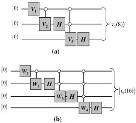
Figure 2: Quantum circuit (a) is for preparing of the three-qubit test state $|t_{0}(8)\rangle$ and (b) is for the four-qubit test state $|t_{0}(16)\rangle$, respectively. Here, the input state is $|0\rangle^{\otimes n}$ ($n=3,4$), the Hadamard operations are depicted by $H$, and the explicit forms of the various controlled gates (the $V$s and $W$s) are given in the text, where all single-qubit operations are $Y$ rotations.

The quantum circuit displayed in Fig. 2(b) is for the construction of the four-qubit test state $|t_{0}(16)\rangle,$ where $\textit{a}=\sqrt{13/28}$, $\textit{b}=\sqrt{1/28}$, and $a^{2}+15b^{2}=1$. In this case,

$$W_{1}=e^{-i\vartheta_{1}Y}\quad\mbox{with}\enskip\tan\vartheta_{1}=\frac{\sqrt{8}\,b}{\sqrt{a^{2}+7b^{2}}}=\sqrt{\frac{2}{5}}$$ (48)

and

$$W_{2}=e^{-i\vartheta_{2}Y}\quad\mbox{with}\enskip\tan\vartheta_{2}=\frac{\sqrt{a^{2}+3b^{2}}-2b}{\sqrt{a^{2}+3b^{2}}+2b}=\frac{1}{3}$$ (49)

as well as $W_{3}=V_{2}$ and $W_{4}=V_{3}$.

The generalization to the $n$-qubit case is immediate. How to efficiently split a multi-qubit controlled unitary operation $C^{n-1}(V)$ (single-qubit gate $V$ with ${n-1}$ control qubits) in terms of universal gates with $n-1$ work qubits is shown in Refs. gate ; QCQI , and its circuit complexity is of the order of $n$. Consequently, the circuit complexity for constructing the $n$-qubit test state with quantum circuits of the kind shown in Fig. 2 is $O(n^{2})$. In Appendix B, an alternative method for constructing the test state $|t_{0}\rangle$ is given, where the amplitudes $a$ and $b$ are complex numbers.

VI.2 Realization of the SRM

In order to perform the SRM of Sec. III.1 in the laboratory, one needs a unitary transformation

$$\textbf{M}=\sum_{l=0}^{N-1}|l\rangle\langle T_{0}^{l}|$$ (50)

that turns each basis ket $|T_{0}^{l}\rangle$ into the corresponding ket $|l\rangle$ of the computational basis. With Eqs. (11) and (20) we have

$$\textbf{M}=-\mathcal{I}+(1-a)|0\rangle\langle 0|+b\bigl{(}|0\rangle\langle v|+|v\rangle\langle 0|\bigr{)}+y|v\rangle\langle v|$$

$$\mbox{with}\ |v\rangle=\sum_{k=1}^{N-1}|k\rangle\,,$$ (51)

which has one eigenvalue $+1$ and ${N-1}$ eigenvalues $-1$, so that the unitary operators $-\textbf{M}$ and the $n$-qubit-controlled-$Z$

$$C^{n-1}(Z)=\mathcal{I}-2|N-1\rangle\langle N-1|=\mathcal{O}^{N-1}$$ (52)

have the same set of eigenvalues, that is: they are unitarily equivalent. The eigenkets of M are

$$|e_{0}\rangle = \sqrt{\frac{1-a}{2}}|0\rangle+\frac{b}{\sqrt{2(1-a)}}|v\rangle\,,$$

$$|e_{1}\rangle = -\sqrt{\frac{1+a}{2}}|0\rangle+\frac{b}{\sqrt{2(1+a)}}|v\rangle\,,$$

$$|e_{j}\rangle = \frac{1}{\sqrt{2}}\bigl{(}-|1\rangle+|j\rangle\bigr{)}\quad\mbox{for}\enskip j=2,3,\dots,N-1\,,\qquad$$ (53)

with $\textbf{M}|e_{0}\rangle=|e_{0}\rangle$ and $\textbf{M}|e_{j\neq 0}\rangle=-|e_{j\neq 0}\rangle$. In view of the degeneracy of M, the set of orthonormal eigenkets for eigenvalue $-1$ is not unique, but the choice of Eqs. (VI.2) is particularly useful in the present context. For, the eigenket $|e_{0}\rangle$ has the same structure as the test state $|t_{0}\rangle$ of Eq. (10), and we know from Sec. VI.1 how to construct $|t_{0}\rangle$.

We relate M to $C^{n-1}(Z)$ through the unitary operator $\textbf{U}\,X^{\otimes n}$ that diagonalizes M in the computational basis,

$$\textbf{M}=-\textbf{U}\,X^{\otimes n}\,C^{n-1}(Z)\,X^{\otimes n}\,\textbf{U}^{\dagger}$$ (54)

The operator U itself is such that $\textbf{U}|0\rangle^{\otimes n}=|e_{0}\rangle$ or $\textbf{U}\,X^{\otimes n}|1\rangle^{\otimes n}=|e_{0}\rangle$, and we realize it by the circuit for u—see Fig. 2—with the replacements

$$a \rightarrow \sqrt{(1-a)/2},$$

$$b \rightarrow b/\sqrt{2(1-a)}\,,$$ (55)

while $\textbf{U}^{\dagger}$ is implemented by the circuit that has the gates of Fig. 2 in reverse order and all respective $\theta$ angle parameters replaced by $-\theta$. Accordingly, all unitary factors on the right-hand side of Eq. (54) have known realizations, as illustrated for $N=2^{3}$ in Fig. 3.

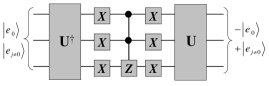
Figure 3: The quantum circuit for the implementation of $-\textbf{M}$ in the case of three qubits. The operation U is implemented by the circuit shown in Fig. 2(a) after changing the parameters in accordance with Eq. (VI.2). And, if we run the same circuit in the reverse order we can also implement $\textbf{U}^{\dagger}$. The quantum gate shown in the center of circuit is the $C^{2}(Z)$ given by Eq. (52).

With the SRM measurement thus implemented and the corresponding test states of Sec. VI.1, we can verify the GA outcome and complete the quantum search as discussed in Sec. IV, and we can also perform the full-space test-state search of Sec. V, for which Eqs. (V) and (39) apply. Of course, there are implementations as well of the test states in successively smaller spaces and of the corresponding SRM measurements, but we are not aware of economic implementations. The restriction to the subspaces of yet-to-probe index states is rather awkward in practice.

VII Summary and discussion

We have introduced the test states that enable one to verify whether the outcome of a quantum search with the Grover’s algorithm is the actual oracle or not. We thereby regard the search problem as defined by the set of possible oracles, which are those considered by Grover. Other search problems, such as the one studied by Høyer extGA , are not automatically covered as well; the corresponding test states—if they exist—have to be found for each search problem separately. That is also the case for Grover-type searches with more than one matching item, that is when the oracle is a product of two or more different unitary operators of the kind defined in Eq. (4).

It is possible that there are no test states for some of these other search problems, in which case one may not be able to verify if the search was successful — neither by test states of some sort, nor by a method like the one described in Appendix A below, nor by another procedure. This should make one wonder if a search problem is well-posed in the first place, if it is not possible to verify the outcome. We leave this as a moot point.

With the test states at hand, we have the option of solving the quantum search problem with a classical search strategy. But there is a twist: While there is one “yes” answer, each “no” answer is slightly different and, with the help of the square-root measurement, this difference can be exploited systematically for a judicious choice of the test state for the next round. This educated guessing is rewarded by much fewer queries of the oracle on average than what one needs for the simple “yes/no” search. A reduction by a factor of $3.41$ is achievable in principle, and a practical scheme still gains a factor of more than three. In our view, the classical-search benchmark is set by the search that exploits the differences between the “no”s fully.

The picture is completed by giving explicit circuits for the implementation of the $n$-qubit test states. The circuit complexity is of order $n^{2}$, and a variant of the same circuit is the main ingredient in the realization of the square-root measurement.

Appendix A An alternative confirmation step for Grover’s algorithm

Here we describe an alternative procedure for verifying the result obtained by GA. This method does not rely on the construction of test states. Rather it employs a simple circuit that distinguishes between two selected “target oracles” and the other ${N-2}$ oracles. The verification is achieved by having the GA-outcome oracle in two different target pairs, and thus requires two queries of the oracle.

Suppose GA has had oracle $\mathcal{O}^{j}$ as the outcome. The corresponding index ket $|j\rangle=|x_{1}\chi\rangle$ has value $x_{1}$ for the first qubit and the values of qubits $2$,$3$, …, $n$ are summarized by the string $\chi$. We pair $|j\rangle$ with $|\widehat{j}\rangle=|\widehat{x_{1}}\chi\rangle$ where

$$\widehat{x_{1}}=x_{1}+1\ (\mbox{mod}\ 2)=\left\{\begin{array}[]{l@{\ \mbox{if}\ }l}1&x_{1}=0\,,\\[4.30554pt] 0&x_{1}=1\,,\end{array}\right.$$ (56)

so that $j$ and $\widehat{j}$ differ in the first bit value only.

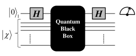
Figure 4: A single iteration of the alternative confirmation is exhibited in terms of quantum circuit diagram. The input state with ket $|\phi_{\textrm{in}}\rangle=|0\chi\rangle$ of Eq. (57) is passed through the sequence of the Hadamard gate $H$ of Eq. (5), the quantum black box, and another Hadamard gate. Finally, the 1st qubit of the output state $|\phi_{\textrm{out}}\rangle$ is measured in the computational basis.

As indicated in Fig. 4, we prepare qubit 1 in the state with ket $|0\rangle$, and encode the $\chi$ part of the index state in qubits $2$ through $n$. So, the ket of the $n$-qubit input state is

$$|\phi_{\textrm{in}}\rangle=|0\chi\rangle=\left\{\begin{array}[]{l@{\ \mbox{if}\ }l}|j\rangle&x_{1}=0\,,\\[4.30554pt] |\widehat{j}\rangle&x_{1}=1\,.\end{array}\right.$$ (57)

We pass it through the quantum circuit of Fig. 4, where the given black box is used only once. If the black box is implementing either oracle $\mathcal{O}^{j}$ or oracle $\mathcal{O}^{\widehat{j}}$, then the output state will have ket

$$|\phi^{\mathrm{(yes)}}_{\textrm{out}}\rangle=|1\chi\rangle\,.$$ (58)

If, however, the black box is implementing one of the other ${N-2}$ oracles, the output state will have ket

$$|\phi^{\mathrm{(no)}}_{\textrm{out}}\rangle=|0\chi\rangle\,.$$ (59)

Finally, qubit 1 is measured in the computational basis. If we find $0$, the “no” output is the case, and we can be sure that the actual oracle is neither $\mathcal{O}^{j}$ nor $\mathcal{O}^{\widehat{j}}$. But when we find $1$, we know that one of these oracles is inside the black box. We determine which one by pairing $|j\rangle$ with a third index ket that also differs only by the value of one qubit, which then plays the role of the privileged qubit in the corresponding circuit of the kind depicted in Fig. 4, where qubit 1 is singled out.

So, we either get a definite “no” answer to the question “Is the $j$th or the $\widehat{j}$th oracle the case?” or we are told “yes, it is one of these two.” In the latter situation, we know for sure which one it is after a second round.

Appendix B An alternative construction of the test states

In Sec. VI.1, we gave a construction of the test states of Eq. (10) with the real coefficients $a$ and $b$ of Eq. (15). Here, we provide an alternative method by which one produces the alternative test states with complex $a$ and $b$ amplitudes, as exemplified by

$$|t_{0}\rangle = a|0\rangle+b\sum_{l=1}^{N-1}|l\rangle$$ (60)

$$= (a-b)|0\rangle^{\otimes n}+b\sqrt{N}|+\rangle^{\otimes n}\,,$$

where $|+\rangle=H|0\rangle=\bigl{(}|0\rangle+|1\rangle\bigr{)}/\sqrt{2}$ uses the Hadamard gate of Eq. (5), and the absolute values $|a|$ and $|b|$ are, of course, still those of Eq. (15). As before, it is enough to show how $|t_{0}\rangle$ is made, the other test states are then available by applying some single-qubit $X$ gates.

We obtain a ket of this kind by applying the multi-Hadamard unitary operator

$$U^{12\dots n}_{HH...H}(\theta)=\exp\bigl{(}-i\theta H^{\otimes n}/2\bigr{)}\,,$$ (61)

to $|j=0\rangle=|0\rangle^{\otimes n}$,

$$U^{12\dots n}_{HH\dots H}(\theta)|0\rangle^{\otimes n}=\cos\frac{\theta}{2}\,|0\rangle^{\otimes n}-i\sin\frac{\theta}{2}\,|+\rangle^{\otimes n}\,.$$ (62)

Now, for $b\sqrt{N}=-i\sin(\theta/2)=-i\sqrt{N/(2N-4)}$ we need to set the angle parameter $\theta$ to the value determined by

$$\tan\frac{\theta}{2}=\sqrt{\frac{N}{N-4}}\,,$$ (63)

and one verifies that

$$a=\cos\frac{\theta}{2}-\frac{i}{\sqrt{N}}\sin\frac{\theta}{2}=\frac{\sqrt{N-4}-i}{\sqrt{2N-4}}$$ (64)

also has the absolute value required by Eq. (15). So, if we set $\theta$ in accordance with Eq. (63), then the output state of Eq. (62) is the test state $|t_{0}\rangle$ of Eq. (60). We note that $\theta=\pi$ for $N=4$, and $\theta=\pi/2+2/N$ for $N\gg 1$.

One can execute the unitary operation $U^{12\dots n}_{HH\dots H}(\theta)$ on the $n$-qubit input state $|0\rangle^{\otimes n}$ by a similar method as the one given for the unitary operation $U^{12\dots n}_{ZZ\dots Z}(\theta)$ in Sec. IIA of Ref. HQCM . Here, the input quantum register of $n$ qubits (circles in Fig. 5(i)) and the ancilla qubit ‘$r$’ (diamond in Fig. 5(i)) are initialized in the $n$-qubit input state with ket $|0\rangle^{\otimes n}$ and the state with ket $|+\rangle_{r}$, respectively. Then, similar to the $n$ cz operations in Sec. II A of Ref. HQCM , here we perform the $n$ controlled-Hadamard operations

$$\textsc{ch}(n)=\bigl{(}|0\rangle\langle 0|\bigr{)}_{r}\otimes I^{\otimes n}+\bigl{(}|1\rangle\langle 1|\bigr{)}_{r}\otimes H^{\otimes n}$$ (65)

between the ancilla qubit and each one of the $n$ qubits. All the controlled-Hadamard operations represented by the bonds in Fig. 5(i) can be carried out at the same time, because they all commute with each other. This leads us to the resultant star-graph state with the ket

$$|\phi\rangle_{(1+n)}=\frac{1}{\sqrt{2}}\bigl{(}|0\rangle_{r}\otimes|0\rangle^{\otimes n}+|1\rangle_{r}\otimes|+\rangle^{\otimes n}\bigr{)}\,.$$ (66)

The subscript $1+n$ reveals the number of qubits of the final graph state.

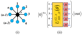
Figure 5: (Color online) (i) The “star graph” stands for the graph state with the ket $|\phi\rangle_{(1+n)}$ of Eq. (66). The (blue) circles represent the $n$ qubits which carry the input ket $|0\rangle^{\otimes n}$; the bonds are established by the controlled-Hadamard gates $\textsc{ch}(n)$ of Eq. (65), and the ancilla qubit ‘$r$’ is represented by the (black) diamond. Plot (ii) represents the net effect on the input ket $|0\rangle^{\otimes n}$, when the ancilla qubit is measured in an appropriately chosen basis.

A single-qubit projective measurement on the ancilla qubit ‘$r$’ in the basis

$$|\!\uparrow(\theta,\tfrac{1}{2}\pi)\rangle_{r} = \cos\frac{\theta}{2}\,|0\rangle_{r}+i\sin\frac{\theta}{2}\,|1\rangle_{r}\,,$$

$$|\!\downarrow(\theta,\tfrac{1}{2}\pi)\rangle_{r} = -\sin\frac{\theta}{2}\,|0\rangle_{r}+i\cos\frac{\theta}{2}\,|1\rangle_{r}$$ (67)

transforms the input ket of the $n$ qubits into the ket

$$|\mathrm{out}\rangle=\bigl{(}H^{\otimes n}\bigr{)}^{m_{r}}U^{12\dots n}_{HH\dots H}(\theta)|0\rangle^{\otimes n}\,.$$ (68)

Here, $m_{r}\in\left\{0,1\right\}$ is the measurement result, and $\bigl{(}H^{\otimes n}\bigr{)}^{m_{r}}$ is the byproduct operator Raussendorf01 ; Raussendorf011 , which is represented by the dotted boxes on all the $n$ qubits in Fig. 5(ii).

After undoing the effect of the byproduct operator in Eq. (68), one has the test state of Eq. (60), and can then apply the necessary single-qubit $X$ gates to get the test state that one needs. Alternatively and more efficiently, one can combine these $X$ gates with the byproduct operator and execute the resulting single-qubit gates in one go.

References

- (1) D. Deutsch, Proc. R. Soc. London Ser. A 400, 97 (1985).
- (2) D. Deutsch, Proc. R. Soc. London Ser. A 425, 73 (1989).
- (3) D.P. DiVincenzo, Science 270, 255 (1995).
- (4) C.H. Bennett and P.W. Shor, IEEE Trans. Inf. Theory 44, 2724 (1998).
- (5) C.H. Bennett and D.P. DiVincenzo, Nature (London)404, 247 (2000).
- (6) D.E. Knuth, The Art of Computer Programming, Vol. 3, (Addison-Wesley, 3rd edition, 1997).
- (7) L.K. Grover, Phys. Rev. Lett. 79, 325 (1997).
- (8) M.A. Nielsen and I.L. Chuang, Quantum Computation and Quantum Information, (Cambridge University Press, 2007).
- (9) C. Zalka, Phys. Rev. A60, 2746 (1999).
- (10) M. Boyer, G. Brassard, P. Høyer, and A. Tapp, Fortschr. Phys. 46, 493 (1998).
- (11) G. Brassard, P. Høyer, M. Mosca, and A. Tapp, e-print arXiv:quant-ph/0005055.
- (12) P. Høyer, Phys. Rev. A62, 052304 (2000).
- (13) A. Peres, Found. Phys. 20, 1441 (1990).
- (14) A. Peres and W.K. Wootters, Phys. Rev. Lett. 66, 1119 (1991).
- (15) B.-G. Englert and J. Řeháček, J. Mod. Opt. 57, 218 (2010).
- (16) M. Ban, K. Kurokawa, R. Momose, and O. Hirota, Int. J. Theor. Phys. 36, 1269 (1997).
- (17) I.D. Ivanovic, Phys. Lett. A123, 257 (1987).
- (18) R.B.M. Clarke, A. Chefles, S.M. Barnett, and E. Riis, Phys. Rev. A63, 040305(R) (2001).
- (19) A. Barenco, C.H. Bennett, R. Cleve, D.P. DiVicenzo, N. Margolus, P. Shor, T. Sleator, J.A. Smolin, and H. Weinfurter, Phys. Rev. A52, 3457 (1995).
- (20) A. Sehrawat, D. Zemann, and B.-G. Englert, e-print arXiv:quant-ph/1008.1118.
- (21) R. Raussendorf and H.J. Briegel, Phys. Rev. Lett. 86, 5188 (2001).
- (22) R. Raussendorf, D.E. Browne, and H.J. Briegel, Phys. Rev. A68, 022312 (2003).