Cavity versus dot emission in strongly coupled quantum dots–cavity systems

Abstract

We discuss the spectral lineshapes of $N$ quantum dots in strong coupling with the single mode of a microcavity. Nontrivial features are brought by detuning the emitters or probing the direct exciton emission spectrum. We describe dark states, quantum nonlinearities, emission dips and interferences and show how these various effects may coexist, giving rise to highly peculiar lineshapes.

I Introduction

The coherent coupling of a semiconductor quantum dot (QD) exciton to the optical mode of a microcavity has been intensely investigated throughout the last years in cavity quantum electrodynamics (CQED) experiments Yoshie et al. (2004); Reithmaier et al. (2004); Peter et al. (2005); Reitzenstein et al. (2006); Hennessy et al. (2007); Englund et al. (2007); Faraon et al. (2008); Kistner et al. (2008); Winger et al. (2008); Laucht et al. (2009a, b); Münch et al. (2009); Reitzenstein et al. (2009); Ota et al. (2009); Suffczyński et al. (2009); Thon et al. (2009); Nomura et al. (2010); Kasprzak et al. (2010); Laucht et al. (2010a); Dalacu et al. (2010) and theory Andreani et al. (1999); Cui and Raymer (2006); Laussy et al. (2008); Inoue et al. (2008); Naesby et al. (2008); Auffèves et al. (2008); Laussy et al. (2009); del Valle et al. (2009); Yamaguchi et al. (2009); Hughes and Yao (2009); Auffèves et al. (2009); Averkiev et al. (2009); Richter et al. (2009); Vera et al. (2009a, b); Tarel and Savona (2010); Kaer et al. (2010); Hohenester (2010); Ritter et al. (2010); Poddubny et al. (2010). In some of these works, the experimental spectral function of the strongly coupled QD–cavity system was directly compared to a theoretical model Laussy et al. (2008); Laucht et al. (2009b); Münch et al. (2009); Laucht et al. (2010a), and the agreement is excellent. It was assumed that most of the light escapes the system via the radiation pattern of the cavity mode, and the experimental spectra were compared to the spectral function calculated from the cavity occupation. This detection geometry is known in atomic cQED as “end emission” or “forward emission” Yamamoto and Ĭmamoḡlu (1999). In atomic systems, negligible light escapes the cavity through the cavity mode, that is to say, the cavity photon lifetime is so long as to be considered infinite. Light is then detected in the so-called “side-emission”, where the radiation pattern of the emitter is probed instead. With microcavities, the situation is reversed: the cavity mode is measured often with an emitter of a much longer lifetime. In the spontaneous emission regime of a system in strong-coupling, this makes measurements of the Rabi doublet in the photoluminescence more difficult, unless some cavity feeding makes the quantum state of the system photon-like, since changing the nature of the excitation is, in this case, equivalent to changing the channel of detection Laussy et al. (2008). In the nonlinear regime, this also hinders manifestations of the Jaynes–Cummings ladder. All the transitions between its rungs have the same intensity in the exciton emission. In the cavity emission, however, the photon has two paths to be emitted, one with the dot in its ground state, the other with the dot in its excited states del Valle et al. (2009). These two paths interfere destructively when the initial and final states are out of phase, which is the case for two out of the four possible transitions in the Jaynes–Cummings ladder. On the other hand, these two paths interfere constructively when the initial and final states are in phase, or, up to a photon, indistinguishable. In the dressed-state picture, the cavity photon to be emitted decouples from the polaritons and carries away little information from the coupled system, being more like a cavity photon the higher the number of excitations. The dot photon, on the other hand, does not decouple from the system, regardless the number of excitations: the dot cannot de-excite without altering fundamentally the state of the entire system. As a result, the dot photon carries more information of the coupled system. Summarizing, the dot is essentially a quantum emitter whereas the cavity is essentially a classical emitter.

It is therefore interesting to detect directly the dot emission. The ratio $\mathcal{R}$ of dot-vs-cavity emitted photons depends on the populations of the dot (resp. cavity), $n_{1}$ (resp. $n_{a}$) and their rate of emission, $\gamma_{1}$ (resp. $\gamma_{a}$):

$$\mathcal{R}=\frac{n_{1}\gamma_{1}}{n_{a}\gamma_{a}}\,.$$ (1)

This ratio is typically small since—apart from the fact that $0\leq n_{1}\leq 1$ whereas $n_{a}$ is unbounded—in typical experiments, $\gamma_{1}\ll\gamma_{a}$. One should therefore take advantage of the detection geometry, to detect light in a solid angle where the cavity does not emit. In a photonic crystal, one could filter out the areas of most intense cavity emission by selective collection of the farfield emission. The gain is however negligible, the cavity emission being reduced by a factor of about $2$ as compared to the dot emission when one needs several order of magnitude increase to compensate $\mathcal{R}$. The direct dot emission is therefore more easily accessible with pillars Reitzenstein and Forchel (2010), where one can detect on the side of the structure, and where the feasibility of such experiments has already been demonstrated Sanvitto et al. (2006).

In this text, we shall leave away the practical question of detection and discuss the differences that are observed when probing the strong-coupling physics in the cavity and the dot emission. As the possibility of coupling strongly $N>1$ dots to the (one) microcavity mode Yeoman and Meyer (1998); del Valle et al. (2007); Vera et al. (2009c); del Valle (2010a); Poddubny et al. (2010) is starting to emerge experimentally Reitzenstein et al. (2006); Gallardo et al. (2010); Laucht et al. (2010a), we will consider the general case of many emitters. We address both the linear and nonlinear regimes, with incoherent and continuous pumping as the scheme of excitation, which is a favoured way of probing the system experimentally. The effects we will discuss are not limited to the case of quantum dots in a microcavity. Systems with many identical quantum emitters as in atomic physics Thompson et al. (1992); Walther et al. (2006), superconducting qubits Wallraff et al. (2004); Fink et al. (2009); Filipp et al. (2010) or colour centers in diamond Park et al. (2006); Santori et al. (2010); Englund et al. (2010) would also display the phenomenology we report.

II Model

The Hamiltonian for $N$ independent excitons (in different QDs) coupled to a common cavity mode reads

$$H=\sum_{j=1}^{N}\left[{\omega_{j}{\sigma_{j}^{\dagger}}\sigma_{j}}+g_{j}(a^{\dagger}\sigma_{j}+{\sigma_{j}^{\dagger}}a)\right]+\omega_{a}a^{\dagger}a,$$ (2)

where ${\sigma_{j}^{\dagger}}$, $\sigma_{j}$ are the pseudospin operators for the excitonic two level systems consisting of ground state $|0\rangle$ and a single exciton $|X_{j}\rangle$ state of the $j$th–QD. $\omega_{j}$ is the exciton frequency, $a^{\dagger}$ and $a$ are the creation and destruction operators of photons in the cavity mode with frequency $\omega_{a}$, and $g_{j}$ describes the strength of the dipole coupling between cavity mode and exciton of the $j$th–QD. The incoherent loss and gain (pumping) of the dot-cavity system is included in a master equation of the Lindblad form $\frac{d\rho}{dt}=-{i}[H,\rho]+\mathcal{L}(\rho)$, where:

$$\mathcal{L}(\rho) = \sum_{j=1}^{N}\Big{[}\frac{\gamma_{j}}{2}(2\sigma_{j}\rho{\sigma_{j}^{\dagger}}-{\sigma_{j}^{\dagger}}\sigma_{j}\rho-\rho{\sigma_{j}^{\dagger}}\sigma_{j})$$ (3)

$$+\frac{P_{j}}{2}(2{\sigma_{j}^{\dagger}}\rho\sigma_{j}-\sigma_{j}{\sigma_{j}^{\dagger}}\rho-\rho\sigma_{j}{\sigma_{j}^{\dagger}})\Big{]}$$

$$+\frac{\gamma_{a}}{2}(2a\rho a^{\dagger}-a^{\dagger}a\rho-\rho a^{\dagger}a)$$

$$+\frac{P_{a}}{2}(2a^{\dagger}\rho a-aa^{\dagger}\rho-\rho aa^{\dagger})\,.$$

Here, $\gamma_{j}$ is the $j$th exciton decay rate, $P_{j}$ is the rate at which excitons are created by a continuous wave pump laser in the $j$th QD, $\gamma_{a}$ is the cavity loss and $P_{a}$ is the incoherent pumping of the cavity. Pumping of the cavity from non-resonant QDs was observed and investigated by different groups Press et al. (2007); Hennessy et al. (2007); Kaniber et al. (2008); Winger et al. (2009); Suffczyński et al. (2009); Hohenester et al. (2009); Chauvin et al. (2009); Ota et al. (2009); Laucht et al. (2010b). It has been shown how the effective quantum state realized in the system under the interplay of the two types of pumping (cavity and exciton) affects a lot the lineshape Laussy et al. (2008, 2009); del Valle et al. (2009), which, in the linear regime, is a counterpart of the different channels of emission. A pure dephasing rate of the exciton in the $j$th–QD could be included to account for effects originating from high excitation powers or high temperatures Laucht et al. (2009b), which has a tendency to merge together the closely spaced peaks arising from higher rungs emission Gonzalez-Tudela et al. (2010), so we take it negligible for simplicity.

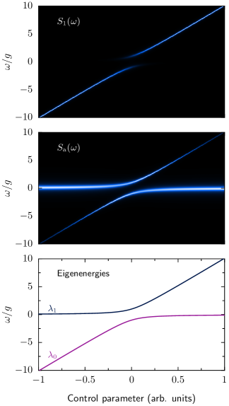
Figure 1: (Colour online) One dot in a cavity. Emission spectrum from the radiation channel of the exciton $S_{1}(\omega)$, from the radiation channel of the cavity mode $S_{a}(\omega)$, and eigenstates of the system. Parameters: $\gamma_{a}/g=0.5$, $\gamma_{1}/g=0.1$, $P_{1}/g=10^{-3}$ and $P_{a}=P_{1}$.

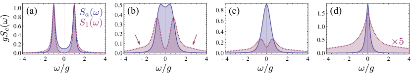
Figure 2: (Colour online) Cavity (solid blue) and dot (dotted purple) emission spectra for one dot in a cavity as a function of pumping power. In the spontaneous emission regime (a), there are no qualitative differences between the two types of spectrum. Increasing pumping (b–d) shows markedly different behaviours in the two channels of emission. Whereas the cavity spectrum does not present a particularly rich phenomenology (collapse of the Rabi doublet), the dot emission displays more characteristic lineshapes. Side elbows are formed [outlined with arrows in (b)] and strong deviations from Lorentzian lines are obtained even when the spectrum has only one peak. Parameters: $\gamma_{a}/g=0.5$, $\gamma_{1}/g=0.1$, $P_{a}=0$ and $P_{1}/g=10^{-3}$, $0.5$, 1 and 2 from left to right panel.

Assuming that the system achieves a steady state for long times and employing the Wiener-Khintchine theorem, we calculate the spectral function of our QD-exciton systems Scully and Zubairy (1997) when photon emission occurs via the normalized radiation pattern of the cavity

$$S_{a}(\omega)=\frac{1}{n_{a}\pi}\lim_{t\rightarrow\infty}\mathrm{Re}\int_{0}^{\infty}d\tau e^{-(\Gamma_{r}-i\omega)\tau}\langle a^{\dagger}(t)a(t+\tau)\rangle,$$ (4)

and via the normalized radiation pattern of the $j$th QD:

$$S_{j}(\omega)=\frac{1}{n_{j}\pi}\lim_{t\rightarrow\infty}\mathrm{Re}\int_{0}^{\infty}d\tau e^{-(\Gamma_{r}-i\omega)\tau}\langle{\sigma_{j}^{\dagger}}(t)\sigma_{j}(t+\tau)\rangle.$$ (5)

We included in the expression the term $\Gamma_{r}$ that takes into account the finite spectral resolution of a monochromator Eberly and Wódkiewicz (1977), which is $\approx$18\text{\,}\mathrm{\SIUnitSymbolMicro}$\mathrm{eV}$ (half-width) for a good monochromator by today standard. The qualitative effect of this term is to broaden the peaks and blur the features. Therefore, in the following we shall assume it is zero (case of a perfect detector).

Using the quantum regression theorem Carmichael et al. (1989), the emission eigenfrequency is obtained by solving the Liouvillian equations for the single time expectation value, and has been amply detailed elsewhere del Valle (2010b). Assuming that the emission energy of different QDs change differently with respect to a control parameter, which is the case for electrically tuning QDs, we can bring two or more QDs at resonance at the same time. This can be simply modeled by an effective control parameter such as $\omega_{j}=\alpha_{j}V_{\mathrm{control}}$, where $\alpha_{j}$ gives the different slopes of emission frequency with the control parameter $V_{\mathrm{control}}$. The emission frequency of the cavity mode is assumed not to be affected by this control parameter.

III One emitter

We start with the simplest and most popular case of one QD in strong coupling with the cavity mode. We compare the emission spectra of the cavity and dot emission in Fig. 1, where we plot the emission spectra from the radiation channel of the exciton $S_{1}(\omega)$, from the radiation channel of the cavity mode $S_{a}(\omega)$, and the eigenstates. Close to resonance, both the exciton and the cavity mode emit into both radiation channels and the radiation patterns are very similar (see also Fig. 2(a)). Far away from resonance, the spectra look different, the excitonic channel $S_{1}(\omega)$ being dominated by the emission of the exciton and the cavity channel $S_{a}(\omega)$ being dominated by the cavity emission. However, a difference in the relative emission strengths cannot be directly attributed to a preference in the radiation channel. It is also dependent on the experimental parameters, on the specific pumping rate of the exciton, the number of other transitions or QDs feeding the cavity mode, and of course on the different coupling terms. In the solid state environment the exciton is not only directly coupled to the cavity mode, but also via the phonon bath Hohenester et al. (2009); Hohenester (2010); Kaer et al. (2010); Hughes et al. (2011).

Increasing pumping, one reaches the nonlinear regime and climbs the Jaynes–Cummings ladder del Valle et al. (2009). In the cavity emission, at resonance, in a typical system where the coupling strength is not much larger than the decay rates, this transition results in an apparent collapse of the Rabi doublet into a single line. If the number of photons is high enough, this line narrows as a consequence of the cavity entering the lasing regime. This transition, displayed in solid blue in Fig. 2, has been reported experimentally Nomura et al. (2010). Its counterpart in the dot emission (purple dotted line) is richer in qualitative features in the nonlinear regime del Valle et al. (2009). This manifests by the elbows in Fig. 2(b-d) [indicated by arrows in (b)], that arise from the transitions $\left|n,\pm\right\rangle\rightarrow\left|n-1,\mp\right\rangle$, that are suppressed in the cavity emission. We have used the standard notation for the eigenstates of the Jaynes–Cummings Hamiltonian with $\left|n,\pm\right\rangle$ the state with $n$ excitation of higher ($+$) and lower ($-$) energy. In the lasing regime, (d), the dot emission is strongly non-Lorentzian and exhibits a characteristic lineshape reminiscent of the one-atom laser del Valle and Laussy (2010).

A simple and convenient way to evidence Jaynes–Cummings nonlinearities is to bring the system out of resonance. In this way, transitions that are otherwise closely packed together, can be put apart and resolved in the photoluminescence spectrum. This is shown in Fig. 3 for the same system as previously but detuning the two bare emitters from each other by $\Delta=\omega_{a}-\omega_{1}$. The Rabi doublet at resonance turns into a triplet at small detunings. This is because one of the transitions $\left|2,\pm\right\rangle\rightarrow\left|1,\pm\right\rangle$—that are too broad and too close from the linear transitions $\left|1,\pm\right\rangle\rightarrow\left|\text{vacuum}\right\rangle$ at resonance—can be set apart at a small detuning, as shown in the lower panel (a-b).

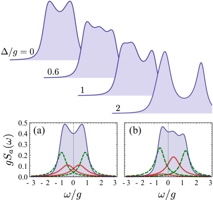
Figure 3: (Colour online) Cavity spectrum of one dot in a cavity as a function of detuning. Lower panels, decomposition of the spectrum in its dressed states emission lines ($\left|1,\pm\right\rangle\rightarrow\left|\mathrm{vacuum}\right\rangle$ in dashed green and $\left|2,\pm\right\rangle\rightarrow\left|1,\pm\right\rangle$ in dotted red), showing how (a) Jaynes–Cummings transitions are hindered at resonances but (b) are revealed out of resonance. Parameters are the same as in Fig. 2 but with the detunings $\Delta/g=0$, $0.6$, $1$ and $2$ and $P_{1}/g=0.4$.

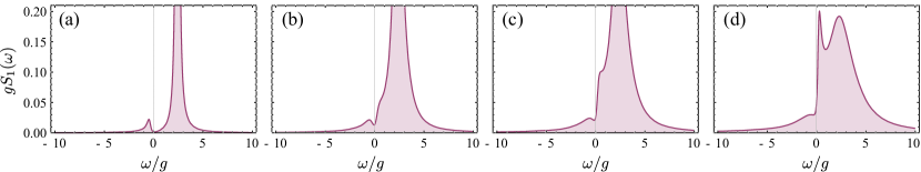
Figure 4: (Colour online) Dot emission spectrum of one dot in a cavity, out of resonance, as a function of pumping. The Rabi doublet in the spontaneous emission regime (a) gives rise, with increasing pumping (b–d), to an emission dip: the incoherent excitation is coherently scattered to the cavity which enters the lasing regime. This is better seen at nonzero detuning. Parameters are the same as in Fig. 2 but for $\Delta=2g$.

Transitions between dressed states provide a faithful mapping to the exact system dynamics when the system is in very strong coupling, so that dressed states are well defined and do not overlap appreciably with each other. In the case where they overlap, say because the splitting between dressed states is small or because their broadening is large, interferences between the states enter the picture. The luminescence can indeed be decomposed as a sum of Lorentzian emissions from the dressed states with dispersive corrections arising from each dressed states driving or being driven by the others del Valle et al. (2009). These interferences can become particularly strong and complex when the system is brought towards the classical regime, that is, with a lot of excitations. In this case, many dressed states enter the collective dynamics, and their overlap as well as mutual disturbance are thus much stronger.

This effect is also better seen at nonzero detuning. Although the interference grows with pumping also at resonance, it tends to be cancelled by symmetry: dressed states from both sides of the origin (set at the bare cavity emission) equilibrate each other. With detuning, however, imbalance magnifies the interferences, that may manifest strikingly. This is shown for instance in Fig. 4 that reproduces Fig. 2 (for the dot emission only) but at detuning $\Delta=2g$. The figure shows how, as pumping is increased, an emission dip develops at the origin as the lines broaden. It starts to be particularly visible in panel (b) whereas, at low excitation [panel (a)], one merely sees the exciton, detuned, favouring its own mode of radiation, just as in the linear case (cf. Fig. 1). Note how, at resonance, in Fig. 2, this interference is masked, being essentially cancelled by symmetry.

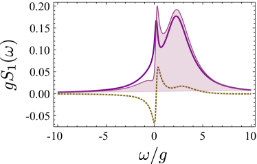
Figure 5: (Colour online) Detail of Fig. 4(d). The interference that arises as the system enters lasing is best seen in the detuned system because dressed states (solid purple) are then of a markedly different character, cf. the exciton line broadened by pumping, right, and the narrow line of the cavity that enters lasing (origin). The interferences between dressed states (dotted brown), which added to the dressed state emission provide the PL spectrum (filled purple), strongly modify the results of kinetic theory applied to the dressed states.

The physical meaning of this dip can be assigned, in this case, to the cavity entering the lasing regime at this frequency, and therefore sucking-up excitations from the quantum dot, that is the medium providing them. In Fig. 5, we show a decomposition of Fig. 4(d) into the sum of dressed states emission (thick solid purple) and the sum of interferences between the dressed states (dashed brown). The observed PL spectrum is the sum of these two contributions, obtained from a mathematical decomposition of the $G^{(1)}(t,\tau)=\langle{a^{\dagger}}(t)a(t+\tau)\rangle$ into terms that give rise to Lorentzian lines (identifying the dressed states) and to dispersive interferences when the dressed state emissions overlap del Valle et al. (2009). The final result can be adequately described by the dressed states only whenever interferences between them are negligible, that is, when they do not overlap. This is the case at low excitation and in the very strong coupling regime, when $g\gg\gamma_{a},\gamma_{1}$ and the splitting to broadening ratio of all transitions is large. In this case, a kinetic theory that computes mean occupation of the dressed states with rate (Boltzmann) equations is adequate Poddubny et al. (2010). Otherwise, a full master equation approach is required, although it quickly becomes untractable. As the intensity is further increased, interferences result in the breakdown of the dressed state picture when the system acquires some macroscopic coherence. Analytical investigations show that the emission dip corresponds to a coherent scattering peak from the dot to the cavity, which, in some approximations, becomes a Dirac $\delta$ function, that describes Rayleigh scattering del Valle and Laussy (2010).

IV More than one emitter

The dynamics of strongly-coupled and strongly dissipative systems becomes very complex as new paths of coherence flow between the dressed states are opened by pumping and decay. This can give rises to new peaks (of emission or absorption) not accounted for by the dressed state picture del Valle (2010c).

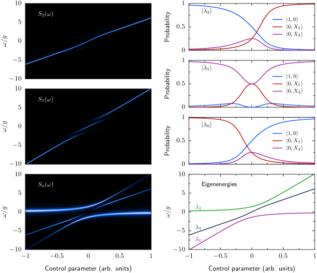
Figure 6: (Colour online) Emission spectrum from the radiation channel of the first exciton $S_{1}(\omega)$, the second exciton $S_{2}(\omega)$, the cavity mode $S_{a}(\omega)$, and the eigenstates for a strongly coupled system of two excitons and the cavity mode. The eigenvectors of the three eigenstates $\left|\lambda_{2}\right\rangle$, $\left|\lambda_{1}\right\rangle$, and $\left|\lambda_{0}\right\rangle$ of the coupled system display the contributions of the individual quantum states $\left|1,0\right\rangle$, $\left|0,X_{1}\right\rangle$, and $\left|0,X_{2}\right\rangle$ to the specific eigenstate. Parameters: same as in Fig. 1 with identical pumping of the dots.

At low pumping, when all $N$-QDs excitons are exactly at resonance with the cavity mode, the eigenvalues and eigenstates of the system (neglecting incoherent loss, and setting the origin of the energy scale to $\omega_{a}$) have a simple and well known form Mandel and Wolf (1995): two are splitted in energy, $\lambda_{\begin{subarray}{c}N\\ 0\end{subarray}}=\pm\Omega$ where $\Omega=\sqrt{\sum_{j=1}^{N}g_{j}^{2}}$, while the other $N-1$ are degenerated and equal to $0$. The corresponding eigenstates are:

$$|\lambda_{\begin{subarray}{c}N\\ 0\end{subarray}}\rangle=\frac{1}{\sqrt{2}}\left(\sum_{j=1}^{N}\frac{g_{j}}{\Omega}|0,X_{j}\rangle\pm|1,0\rangle\right)\,,$$ (6a)

$$|\lambda_{j-1}\rangle=\frac{1}{\Omega_{j}}\big{(}g_{1}|0,X_{j}\rangle-g_{j}|1,0\rangle\big{)}\,,$$ (6b)

with $\Omega_{j}=\sqrt{g_{1}^{2}+g_{j}^{2}}$, with $j$ ranging from $2$ to $N$ for the degenerated eigenstates (6b). From this solution we can see that only the $\left|\lambda_{\begin{subarray}{c}N\\ 0\end{subarray}}\right\rangle$ states have a contribution from the cavity photons. The cavity mode does not contribute to the other states $\left|\lambda_{j-1}\right\rangle$ which are called, for this reason, dark states. They consequently cannot be probed in the cavity spectrum $S_{a}(\omega)$, but they can be very well seen in the excitonic radiation channel or a mixture of all radiation channels. These superpositions also give rise to the phenomenon of sub- and superradiance, first reported by Dicke Dicke (1954). This is essentially a classical effect, that is also observed with vibrating strings. Recently, such configurations have been analyzed in the microcavity QED context by Temnov and Woggon Temnov and Woggon (2009), who studied the photon statistics, and by Poddubny et al. Poddubny et al. (2010), who studied the PL lineshapes. The latter authors found that this classical regime is particularly fragile to incoherent pumping since dark states, being also excited by pumping, act as a long-lived reservoir for bright states from higher manifolds. They also analyzed the regime of very high excitations, when the system is (or is going towards) lasing. They observe in such a case that, due to the predominance of the Dicke states that are the most highly degenerated, the cavity spectrum is either oddly or evenly peaked depending on the parity of the number of strongly coupled dots, which is a strong manifestation in a readily measured observable of the underlying microscopic configuration. In the following, we address particular cases of larger than one, but still small number (given the difficulty in coupling larger assemblies) of dots and show how, in the linear regime, photoluminescence spectra vary greatly in a qualitative way because of the contribution or suppression of the dark states. We confirm that these states are quickly spoiled with increasing pumping Poddubny et al. (2010) and give rise to nonlinear quantum features, that also manifest in strikingly different ways depending on the radiation channel that is probed.

IV.1 Two emitters

In the case of two emitters coupled to a single cavity mode, the eigenfrequencies in the linear regime can be obtained by solving the eigenvalue problem given by the following equation:

$$i\frac{\partial}{\partial t}\begin{pmatrix}\langle a\rangle\\ \langle\sigma_{-}^{1}\rangle\\ \langle\sigma_{-}^{2}\rangle\end{pmatrix}=\begin{pmatrix}\tilde{\omega}_{a}&g_{1}&g_{2}\\ g_{1}&\tilde{\omega}_{1}&0\\ g_{2}&0&\tilde{\omega}_{2}\end{pmatrix}\begin{pmatrix}\langle a\rangle\\ \langle\sigma_{-}^{1}\rangle\\ \langle\sigma_{-}^{2}\rangle\end{pmatrix}$$ (7)

where $\tilde{\omega}_{a}=\omega_{a}-i\Gamma_{a}/2$ and $\tilde{\omega}_{j}=\omega_{j}-i\Gamma_{j}/2$, with $\Gamma_{a}=\gamma_{a}-P_{a}$, and $\Gamma_{j}=\gamma_{j}+P_{j}$. From the eigenstate of the emission eigenfrequency we can obtain the degree of mixture of each peak in the spectrum, i.e., the strength of the contribution of the cavity mode, QD1 exciton and QD2 exciton to each individual eigenstate.

In Fig. 6, we investigate a system of two excitons in different QDs simultaneously coupled to one cavity mode. We compare the emission spectra obtained via the radiation channel of the first exciton $S_{1}(\omega)$, the second exciton $S_{2}(\omega)$ and the cavity mode $S_{a}(\omega)$. In the spontaneous emission regime, while all three radiation channels exhibit a markedly different emission spectrum, the most striking difference can be found in $S_{a}(\omega)$ where one of the emission lines vanishes completely. This occurs when subradiance sets in, and follows for the case of two emitters an analysis of the eigenvectors similar to that of Ref. Laucht et al. (2010a). The plot of the eigenvectors in Fig. 6 presents the contributions of the three quantum states $\left|1,0\right\rangle$, $\left|0,X_{1}\right\rangle$, and $\left|0,X_{2}\right\rangle$ to the three eigenstates $\left|\lambda_{2}\right\rangle$, $\left|\lambda_{1}\right\rangle$, and $\left|\lambda_{0}\right\rangle$ (as marked in the plot of the eigenstates) of the coupled system. While $\left|\lambda_{2}\right\rangle$ and $\left|\lambda_{0}\right\rangle$ have contributions from all three quantum states at resonance, for the eigenstate $\left|\lambda_{1}\right\rangle$ the contribution from $\left|1,0\right\rangle$ goes to zero due to destructive interference.

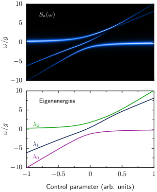
Figure 7: (Colour online) Emission spectrum from the radiation channel of the cavity mode $S_{a}(\omega)$, and eigenstates for a strongly coupled system of two excitons and the cavity mode where the two excitons cross out of resonance from the cavity mode. Parameters: same as in Fig. 6.

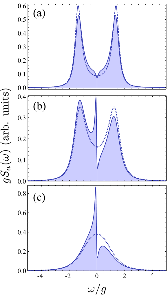
Figure 8: Spectral shapes in the cavity emission when two dots are strongly coupled to the cavity mode. (a) With increasing excitation (solid) the emission dip effect becomes visible in the cavity emission. (b) It is better seen slighly out resonance since it can now “feed” on the line previously cancelled by subradiance. (c) Such interferences are strong even in systems that do not exhibit spontaneous emission features (such as Rabi splitting), altough this still requires strong-coupling. Parameters: $g_{1}=g_{2}=g$ (setting the unit), $\gamma_{a}=g$, $\gamma_{1}=\gamma_{2}=0.1g$, $P_{a}=0$, then: (a) $\Delta_{1}=\Delta_{2}=0$, $P_{1}=10^{-4}g$ with (dotted) $P_{2}=10^{-4}g$ and (solid) $P_{2}=0.1g$. (b) Same as (a) but for $\gamma_{a}=2g$, $P_{1}=10^{-3}g$, $P_{2}=0$, $\Delta_{1}=0$ and (solid) $\Delta_{2}=0.1g$ or (dashed) $\Delta_{2}=0$. (c) Same as (a) but for $\gamma_{a}=5g$, $\Delta_{1}=0$ with (dotted) $\Delta_{2}=0$ or (solid) $\Delta_{2}=0.1g$.

A measurement of this kind would also be possible for the same system as just described, but when the two exciton lines anticross out of resonance from the cavity mode, similar to the system described in Ref. Laucht et al. (2010a). In Fig. 7, we plot the emission spectrum from the radiation channel of the cavity mode $S_{a}(\omega)$, and the eigenstates of such a system. Probing the cavity emission, one of the emission lines vanishes, similar to the case in Fig. 6, but this time when the two excitons are crossing out of resonance from the cavity mode. In this situation the eigenvalues and eigenstates have also a simple form, $\lambda_{1}=\Delta$, $\lambda_{\begin{subarray}{c}2\\ 0\end{subarray}}=\Delta/2\pm\sqrt{\Delta^{2}+4(g_{1}^{2}+g_{2}^{2})}/2$, with $\Delta=\omega_{1}-\omega_{a}$ being the mutual detuning from the cavity mode. In this case, the eigenstates are:

$$|\lambda_{\begin{subarray}{c}2\\ 0\end{subarray}}\rangle=\frac{1}{\sqrt{(\lambda_{\begin{subarray}{c}2\\ 0\end{subarray}})^{2}+\Omega_{2}^{2}}}\big{(}g_{1}|0,X_{1}\rangle+g_{2}|0,X_{2}\rangle-\lambda_{\begin{subarray}{c}2\\ 0\end{subarray}}|\mathrm{1,0}\rangle\big{)}\,,$$

$$|\lambda_{1}\rangle=\frac{1}{\Omega_{2}}\big{(}g_{1}|0,X_{2}\rangle-g_{2}|0,X_{1}\rangle\big{)}\,.$$ (8)

Again, since the contribution from the cavity mode to this particular eigenstate ($|\lambda_{1}\rangle$) goes to zero, it cannot be probed by the cavity radiation. The plot of all three eigenstates, however, clearly shows the anticrossing behaviour of the two exciton-like states when they come in resonance detuned from the cavity mode. Laucht et al. (2010a). The disappearance of the second peak during the anticrossing of the excitons brings a clear signature of a collective strong coupling with the two dots and that this is probed in the cavity radiation channel only.

This interference in the linear regime persists in the nonlinear regime where it turns into the interference related to coherence buildup in the system, as was the case with one dot in the cavity, cf. Figs. 4-5. Such interferences are, however, now directly accessible through the cavity spectrum, whereas they were previously only to be seen in the dot emission, which is technically more challenging. This is shown in Fig. 8, at resonance (a) and out of resonance (b-c). The sharp line near the origin in panels (b) and (c) is the exciton line that appears suddenly as subradiance cancellation is destroyed by going out of resonance, cf. Fig. 6. It results from the interplay of subradiance and detuning, studied in Ref. Averkiev et al. (2009), and the method outlined there, in the linear regime, indeed reproduces such spectral features. In the nonlinear regime, this line also suffers from the dip carved by the cavity, where it is sharply located. This effect is robust regardless of the broadening of the cavity, i.e., with and without observation of the Rabi doublet. Here again, detuning is paramount in revealing the underlying physics, as seen in (b-c) where the resonant case is superimposed as dotted line: a very small dip at $\omega=0$ is hardly visible at resonance [similar to the solid line in panel (a)], in contrast to the detuned case that produces a huge jump in the spectral shape.

IV.2 Three emitters and beyond

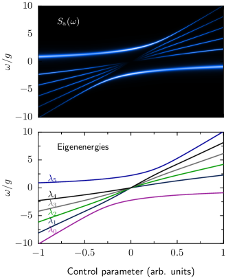
Figure 9: (Colour online) Emission spectrum from the radiation channel of the cavity mode $S_{a}(\omega)$ and the eigenstates of a strongly coupled system of five QD excitons and the cavity mode. Parameters: same as in Fig. 6.

In the linear regime, the interference in the cavity emission due to settling of dark states simply scales in the expected way with the number of dots, by the very nature of linearity. As many lines vanish as there are corresponding strongly coupled dots (minus one). Exemplarily, we simulate the spectral shapes of a system of five identical quantum emitters coupled to the same cavity mode and plot in Fig. 9 the emission spectrum from the radiation channel of the cavity mode $S_{a}(\omega)$ and the corresponding eigenvalues. At resonance, the cavity radiation channel shows only the anticrossing of two of the eigenstates of the coupled system, albeit with a larger splitting corresponding to $2\Omega$, as described before in Eq. (6a).

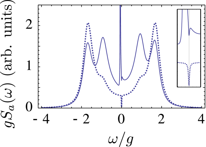
Figure 10: Spectral shapes in the cavity emission when three dots are strongly coupled to the cavity mode for low pumping (dashed line) and high pumping (solid line). This case brings together most features described above. At resonance (dotted), although the emission dip is seen at $\omega=0$, and also the peaks from higher rungs, these are faint and would be difficult to observe with finite detector resolution or counting noise. Detuning the system, (solid), destroys the dark state and gives rise to a sharp line nearby the origin. This one is then strongly affected by the emission dip. Finally, the peaks from nonlinear transitions become much more visible. Inset, zoom around the origin. Parameters: $g_{1}=g_{2}=g_{3}=1$, $\gamma_{a}/g=0.75$, $\gamma_{1}=\gamma_{2}=\gamma_{3}=0.004$, $P_{1}=P_{2}=10^{-6}g$, $P_{3}=0.01g$, $P_{a}=0$ and (dotted) $\Delta/g=0$ or (solid) $\Delta/g=0.1$.

In the nonlinear regime, the situations discussed previously can be reproduced and even brought together, with a higher degree of complexity, by the very nature of nonlinearities. A typical example is shown in Fig. 10 for three emitters, featuring the cavity emission at resonance (thick dotted) and slightly out of resonance (thin solid). In both cases the emission dip is seen at $\omega=0$. In the former case, mainly the Rabi doublet, now at $\pm\sqrt{3}g$, is visible, with less clearly resolved peaks from the transitions of multiply-excited states. Both these features would be lost by finite spectral resolution of the detector. A small detuning breaks the subradiance just like in the linear case and results in the dot eigenstate showing up strongly as a very sharp peak. This also displays the emission dip, like in the case with two dots, as seen in the inset which is a zoom around the origin. This case therefore brings together the two types of strong interferences that manifest in this system: subradiance and emission dip. Note that detuning, which unravels them, also makes much more prominent the peaks that arise from quantum nonlinearities, producing a neat quadruplet, a result we also put forward for the case of one emitter in strong coupling with the cavity.

V Conclusions

We investigated theoretically spectral shapes of $N$ QDs strongly coupled to a single mode of a microcavity, and compared the emission spectra obtained from the two different radiation channels offered by the cavity and direct quantum dot emission, both in the linear and nonlinear regime, at and out of resonance. In the spontaneous emission regime, dark states forming at resonance result in a vanishing of spectral lines in the cavity emission only. When excitation is increased and multiple-photon effects become important, dressed states enter the picture. These are difficult to see in state-of-the-art experiments where splitting to broadening ratio does not allow them to be clearly resolved. Although strong-coupling is maximum at resonance, we find that detuning is an agent to reveal the quantum nonlinear features and that here too dot emission behaves qualitatively differently from cavity emission. As excitation is further increased and a large number of cavity photons is generated (the system enters lasing), another interference due to onset of coherence takes place. It manifests as an emission dip that results from coherent and elastic scattering between the modes. A rich phenomenology thus remains to be observed in these systems. One can access it either by detecting direct dot emission—which is more difficult technically—or by considering strong-coupling involving more than one emitter. In both cases, detuning is a powerful tool to unravel this new physics, since, although optimum, strong-coupling is balanced and/or cancelled at resonance.

We gratefully acknowledge comments from Dr. Poddubny and Dr. Glazov and financial support of the DFG via the SFB 631, Teilprojekt B3, the German Excellence Initiative via NIM, and the EU-FP7 via SOLID. JMVB acknowledges the support of the Alexander von Humboldt Foundation, CAPES, CNPQ and FAPEMIG, EdV of a Newton International fellowship and FPL of the FP7-PEOPLE-2009-IEF project ‘SQOD.’

References

- Yoshie et al. (2004) T. Yoshie, A. Scherer, J. Heindrickson, G. Khitrova, H. M. Gibbs, G. Rupper, C. Ell, O. B. Shchekin, and D. G. Deppe, Nature 432, 200 (2004).
- Reithmaier et al. (2004) J. P. Reithmaier, G. Sek, A. Löffler, C. Hofmann, S. Kuhn, S. Reitzenstein, L. V. Keldysh, V. D. Kulakovskii, T. L. Reinecker, and A. Forchel, Nature 432, 197 (2004).
- Peter et al. (2005) E. Peter, P. Senellart, D. Martrou, A. Lemaître, J. Hours, J. M. Gérard, and J. Bloch, Phys. Rev. Lett. 95, 067401 (2005).
- Reitzenstein et al. (2006) S. Reitzenstein, A. Löffler, C. Hofmann, A. Kubanek, M. Kamp, J. P. Reithmaier, A. Forchel, V. D. Kulakovskii, L. V. Keldysh, I. V. Ponomarev, et al., Opt. Lett. 31, 1738 (2006).
- Hennessy et al. (2007) K. Hennessy, A. Badolato, M. Winger, D. Gerace, M. Atature, S. Gulde, S. Fălt, E. L. Hu, and A. Ĭmamoḡlu, Nature 445, 896 (2007).
- Englund et al. (2007) D. Englund, A. Faraon, I. Fushman, N. Stoltz, P. Petroff, and J. Vučković, Nature 450, 857 (2007).
- Faraon et al. (2008) A. Faraon, I. Fushman, D. Englund, N. Stoltz, P. Petroff, and J. Vuckovic, Nat. Phys. 4, 859 (2008).
- Kistner et al. (2008) C. Kistner, T. Heindel, C. Schneider, A. Rahimi-Iman, S. Reitzenstein, S. Höfling, and A. Forchel, Opt. Express 16, 15006 (2008).
- Winger et al. (2008) M. Winger, A. Badolato, K. J. Hennessy, E. L. Hu, and A. Imamoğlu, Phys. Rev. Lett. 101, 226808 (2008).
- Laucht et al. (2009a) A. Laucht, F. Hofbauer, N. Hauke, J. Angele, S. Stobbe, M. Kaniber, G. Böhm, P. Lodahl, M.-C. Amann, and J. J. Finley, New J. Phys. 11, 023034 (2009a).
- Laucht et al. (2009b) A. Laucht, N. Hauke, J. M. Villas-Bôas, F. Hofbauer, G. Böhm, M. Kaniber, and J. J. Finley, Phys. Rev. Lett. 103, 087405 (2009b).
- Münch et al. (2009) S. Münch, S. Reitzenstein, P. Franeck, A. Löffler, T. Heindel, S. Höfling, L. Worschech, and A. Forchel, Opt. Express 17, 12821 (2009).
- Reitzenstein et al. (2009) S. Reitzenstein, S. Münch, P. Franeck, A. Rahimi-Iman, A. Löffler, S. Höfling, L. Worschech, and A. Forchel, Phys. Rev. Lett. 103, 127401 (2009).
- Ota et al. (2009) Y. Ota, M. Shirane, M. Nomura, N. Kumagai, S. Ishida, S. Iwamoto, S. Yorozu, and Y. Arakawa, Appl. Phys. Lett. 94, 033102 (2009).
- Suffczyński et al. (2009) J. Suffczyński, A. Dousse, K. Gauthron, A. Lemaître, I. Sagnes, L. Lanco, J. Bloch, P. Voisin, and P. Senellart, Phys. Rev. Lett. 103, 027401 (2009).
- Thon et al. (2009) S. M. Thon, M. T. Rakher, H. Kim, J. Gudat, W. T. M. Irvine, P. M. Petroff, and D. Bouwmeester, Appl. Phys. Lett. 94, 111115 (2009).
- Nomura et al. (2010) M. Nomura, N. Kumagai, S. Iwamoto, Y. Ota, and Y. Arakawa, Nat. Phys. 6, 279 (2010).
- Kasprzak et al. (2010) J. Kasprzak, S. Reitzenstein, E. A. Muljarov, C. Kistner, C. Schneider, M. Strauss, S. Höfling, A. Forchel, and W. Langbein, Nat. Mater. 9, 304 (2010).
- Laucht et al. (2010a) A. Laucht, J. Villas-Bôas, S. Stobbe, N. Hauke, F. Hofbauer, G. Böhm, P. Lodahl, M.-C. Amannand, M. Kaniber, and J. J. Finley, Phys. Rev. B 82, 075305 (2010a).
- Dalacu et al. (2010) D. Dalacu, K. Mnaymneh, V. Sazonova, P. J. Poole, G. C. Aers, J. Lapointe, R. Cheriton, A. J. SpringThorpe, and R. Williams, Phys. Rev. B 82, 033301 (2010).
- Andreani et al. (1999) L. C. Andreani, G. Panzarini, and J.-M. Gérard, Phys. Rev. B 60, 13276 (1999).
- Cui and Raymer (2006) G. Cui and M. G. Raymer, Phys. Rev. A 73, 053807 (2006).
- Laussy et al. (2008) F. P. Laussy, E. del Valle, and C. Tejedor, Phys. Rev. Lett. 101, 083601 (2008).
- Inoue et al. (2008) J. I. Inoue, T. Ochiai, and K. Sakoda, Phys. Rev. A 77, 015806 (2008).
- Naesby et al. (2008) A. Naesby, T. Suhr, P. T. Kristensen, and J. Mork, Phys. Rev. A 78, 045802 (2008).
- Auffèves et al. (2008) A. Auffèves, B. Besga, J.-M. Gérard, and J.-P. Poizat, Phys. Rev. A 77, 063833 (2008).
- Laussy et al. (2009) F. P. Laussy, E. del Valle, and C. Tejedor, Phys. Rev. B 79, 235325 (2009).
- del Valle et al. (2009) E. del Valle, F. P. Laussy, and C. Tejedor, Phys. Rev. B 79, 235326 (2009).
- Yamaguchi et al. (2009) M. Yamaguchi, T. Asano, K. Kojima, and S. Noda, Phys. Rev. B 80, 155326 (2009).
- Hughes and Yao (2009) S. Hughes and P. Yao, Opt. Express 17, 3322 (2009).
- Auffèves et al. (2009) A. Auffèves, J.-M. Gérard, and J.-P. Poizat, Phys. Rev. A 79, 053838 (2009).
- Averkiev et al. (2009) N. Averkiev, M. Glazov, and A. Poddubny, Sov. Phys. JETP 135, 959 (2009).
- Richter et al. (2009) M. Richter, A. Carmele, A. Sitek, and A. Knorr, Phys. Rev. Lett. 103, 087407 (2009).
- Vera et al. (2009a) C. A. Vera, H. Vinck-Posada, and A. González, Phys. Rev. B 80, 125302 (2009a).
- Vera et al. (2009b) C. A. Vera, A. Cabo, and A. González, Phys. Rev. Lett. 102, 126404 (2009b).
- Tarel and Savona (2010) G. Tarel and V. Savona, Phys. Rev. B 81, 075305 (2010).
- Kaer et al. (2010) P. Kaer, T. R. Nielsen, P. Lodahl, A.-P. Jauho, and J. Mørk, Phys. Rev. Lett. 104, 157401 (2010).
- Hohenester (2010) U. Hohenester, Phys. Rev. B 81, 155303 (2010).
- Ritter et al. (2010) S. Ritter, P. Gartner, C. Gies, and F. Jahnke, Opt. Express 18, 9909 (2010).
- Poddubny et al. (2010) A. N. Poddubny, M. M. Glazov, and N. S. Averkiev, Phys. Rev. B 82, 205330 (2010).
- Yamamoto and Ĭmamoḡlu (1999) Y. Yamamoto and A. Ĭmamoḡlu, Mesoscopic Quantum Optics (John Wiley & Sons, inc., 1999).
- Reitzenstein and Forchel (2010) S. Reitzenstein and A. Forchel, J. Phys. D: Appl. Phys. 43, 033001 (2010).
- Sanvitto et al. (2006) D. Sanvitto, F. P. Laussy, F. Bello, D. M. Whittaker, A. M. Fox, M. S. Skolnick, A. Tahraoui, P. W. Fry, and M. Hopkinson, arXiv:cond-mat/0612034 (2006).
- Yeoman and Meyer (1998) G. Yeoman and G. M. Meyer, Phys. Rev. A 58, 2518 (1998).
- del Valle et al. (2007) E. del Valle, F. P. Laussy, F. Troiani, and C. Tejedor, Phys. Rev. B 76, 235317 (2007).
- Vera et al. (2009c) C. A. Vera, N. Q. M, H. Vinck-Posada, and B. A. Rodríguez, J. Phys.: Condens. Matter 21, 395603 (2009c).
- del Valle (2010a) E. del Valle, arXiv:1007.1784 (2010a).
- Gallardo et al. (2010) E. Gallardo, L. J. Martinez, A. K. Nowak, D. Sarkar, H. P. van der Meulen, J. M. Calleja, C. Tejedor, I. Prieto, D. Granados, A. G. Taboada, et al., Phys. Rev. B 81, 193301 (2010).
- Thompson et al. (1992) R. J. Thompson, G. Rempe, and H. J. Kimble, Phys. Rev. Lett. 68, 1132 (1992).
- Walther et al. (2006) H. Walther, B. T. H. Varcoe, B.-. Englert, and T. Becker, Rep. Prog. Phys. 69, 1325 (2006).
- Wallraff et al. (2004) A. Wallraff, D. I. Schuster, A. Blais, L. Frunzio, R.-S. Huang, J. Majer, S. Kumar, S. M. Girvin, and R. J. Schoelkopf, Nature 431, 162 (2004).
- Fink et al. (2009) J. M. Fink, R. Bianchetti, M. Baur, M. Goeppl, L. Steffen, S. Filipp, P. J. Leek, A. Blais, and A. Wallraff, Phys. Rev. Lett. 103, 083601 (2009).
- Filipp et al. (2010) S. Filipp, M. Goeppl, J. M. Fink, M. Baur, R. Bianchetti, L. Steffen, and A. Wallraff, arXiv:1011.3732 (2010).
- Park et al. (2006) Y.-S. Park, A. K. Cook, and H. Wang, Nano Letters 6, 2075 (2006).
- Santori et al. (2010) C. Santori, P. E. Barclay, K.-M. C. Fu, R. G. Beausoleil, S. Spillane, and M. Fisch, Nanotechnology 21, 274008 (2010).
- Englund et al. (2010) D. Englund, B. Shields, K. Rivoire, F. Hatami, J. Vuckovic, H. Park, and M. D. Lukin, Nano Letters 10, 3922 (2010).
- Press et al. (2007) D. Press, S. Götzinger, S. Reitzenstein, C. Hofmann, A. Löffler, M. Kamp, A. Forchel, and Y. Yamamoto, Phys. Rev. Lett. 98, 117402 (2007).
- Kaniber et al. (2008) M. Kaniber, A. Laucht, A. Neumann, J. M. Villas-Boas, M. Bichler, M.-C. Amann, and J. J. Finley, Phys. Rev. B 77, 161303(R) (2008).
- Winger et al. (2009) M. Winger, T. Volz, G. Tarel, S. Portolan, A. Badolato, K. J. Hennessy, E. L. Hu, A. Beveratos, J. Finley, V. Savona, et al., Phys. Rev. Lett. 103, 207403 (2009).
- Hohenester et al. (2009) U. Hohenester, A. Laucht, M. Kaniber, N. Hauke, A. Neumann, A. Mohtashami, M. Seliger, M. Bichler, and J. J. Finley, Phys. Rev. B 80, 201311(R) (2009).
- Chauvin et al. (2009) N. Chauvin, C. Zinoni, M. Francardi, A. Gerardino, L. Balet, B. Alloing, L. Li, and A. Fiore, Phys. Rev. B 80, 241306(R) (2009).
- Laucht et al. (2010b) A. Laucht, M. Kaniber, A. Mohtashami, N. Hauke, M. Bichler, and J. J. Finley, Phys. Rev. B 81, 24130(R) (2010b).
- Gonzalez-Tudela et al. (2010) A. Gonzalez-Tudela, E. del Valle, E. Cancellieri, C. Tejedor, D. Sanvitto, and F. P. Laussy, Opt. Express 18, 7002 (2010).
- Scully and Zubairy (1997) M. O. Scully and M. S. Zubairy, Quantum Optics (Cambridge University Press, Cambridge, 1997).
- Eberly and Wódkiewicz (1977) J. H. Eberly and Wódkiewicz, J. Opt. Soc. Am. 67, 1252 (1977).
- Carmichael et al. (1989) H. J. Carmichael, R. J. Brecha, M. G. Raizen, H. J. Kimble, and P. R. Rice, Phys. Rev. A 40, 5516 (1989).
- del Valle (2010b) E. del Valle, Microcavity Quantum Electrodynamics (VDM Verlag, 2010b).
- Hughes et al. (2011) S. Hughes, P. Yao, F. Milde, A. Knorr, D. Dalacu, K. Mnaymneh, V. Sazonova, P. J. Poole, G. C. Aers, J. Lapointe, et al., arXiv:1102.0722 (2011).
- del Valle and Laussy (2010) E. del Valle and F. Laussy, Phys. Rev. Lett. 105, 233601 (2010).
- del Valle (2010c) E. del Valle, Phys. Rev. A 81, 053811 (2010c).
- Mandel and Wolf (1995) L. Mandel and E. Wolf, Optical coherence and quantum optics (Cambridge University Press, 1995).
- Dicke (1954) R. H. Dicke, Phys. Rev. 93, 99 (1954).
- Temnov and Woggon (2009) V. V. Temnov and U. Woggon, Opt. Express 17, 5774 (2009).