Metastable wetting

Abstract.

Consider a droplet of liquid on top of a grooved substrate. The wetting or not of a groove implies the crossing of a potential barrier as the interface has to distort, to hit the bottom of the groove. We start with computing the free energies of the dry and wet states in the context of a simple thermodynamical model before switching to a random microscopic version pertaining to the Solid-on-Solid (SOS) model. For some range in parameter space (Young angle, pressure difference, aspect ratio), the dry and wet states both share the same free energy, which means coexistence. We compute these coexistence lines together with the metastable regions. In the SOS case, we describe the dynamic transition between coexisting states in wetting. We show that the expected time to switch from one state to the other grows exponentially with the free energy barrier between the stable states and the saddle state, proportional to the groove’s width. This random time appears to have an exponential-like distribution.

PACS classification: 68.08.Bc, 68.03.Cd , 05.40.-a.

Keywords: Wetting, metastable, Solid-on-Solid

1. Introduction and outline

The detailed study of superhydrophobic surfaces has revealed that on a rough substrate, a drop can present two shapes: either one obeying the Cassie-Baxter equation or one obeying the Wenzel equation [6], [10], [5]. On the other hand, any transition between two states depends on the height of the barrier which has to be overcome. The corresponding transition will thus be a function of time as revealed already by Kramers law. We review here this crucial aspect of the problem within the framework of an exactly solvable statistical mechanics model. 

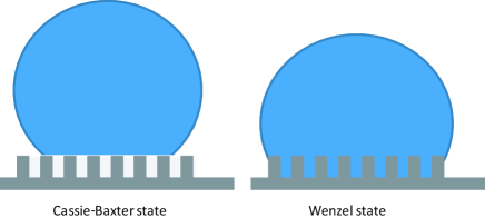
Figure 1. The Cassie-Wenzel states

The corresponding Cassie-Baxter and Wenzel states are illustrated in Fig. 1. In the first (dry) state, there is no wetting of the sides of the U-shaped wells, with vapor trapped in-between, whereas in the second (wet) one, there is at least a partial wetting of the bottom of the U, with vapor trapped in the corners. This is illustrated in Fig. 2, zooming on a single well. The transition between these two states is related to the amplitude of some free-energy barrier: in this rough picture, this barrier can be overcome by applying an external force triggered for instance by an impact velocity or equivalently by increasing the pressure difference $\Delta p$ between liquid and vapor. A classical way to characterize the wet shape is given by the Young contact angle $\theta,$ as sketched on Fig. 2.

A rough substrate is thus made of clefts (wells, grooves…) governing wetting properties. For a better understanding of this physical problem, we need first to analyze and characterize the free energies of both states as functions of the parameters $\theta$, $\Delta p$ and $\rho$, the latter being the shape factor of a typical well. We first do that in Section $2$ for two simple macroscopic solvable models of wetting, one simpler without the pressure parameter and the other one including pressure. For the isotropic model including pressure, we show that there exists a region in parameter space where the two states can both exist (the free energy function has two stable minima) and therefore regions where only a single of these two states exists (the free energy function possesses a single stable minimum). Within the metastable region of existence of the two states, we exhibit a line of coexistence along which the free energies of both states are exactly equal.

We can easily imagine that, due to fluctuations, there will be an opportunity to flip between the ‘dry’ and ‘wet’ states of Fig. 2. So we need to embed our wetting problem into the framework of a stochastic model of wetting. For this purpose, we used the microscopic statistical mechanics SOS model. In this context also, the wetting of a well implies the crossing of a potential barrier: the interface has to distort, to hit the bottom of the well. We wish to understand this problem in more details.

The aim of Section $3$ is to show that we are still able to compute analytically the equilibrium free energies of the dry and wet phases in this statistical SOS context. Let us be more precise. 

We study our wetting problem in the context of the SOS model in a square well of width $l=:nl_{0}$ and height $h,$ with $h/l=:\rho$. The equilibrium measure for the interface heights $h_{i}\geq 0$ is given by:

(1.1) $$d\mu_{n}=Z_{n}^{-1}e^{-\left(J\sum_{i=0}^{n}\left|h_{i+1}-h_{i}\right|+\frac{K}{n}\sum_{i=1}^{n}h_{i}\right)}\prod_{i=0}^{n}\left(1+a\delta\left(h_{i}\right)\right)dh_{i},$$

with $h_{0}=h_{n+1}=h$. Here $Z_{n}$ is the normalizing partition function, and the pressure term comes from $\Delta p\int_{0}^{l}h\left(x\right)dx\simeq\Delta p\sum_{i}h_{i}\frac{l}{n}=\frac{K}{n}\sum h_{i}$, which defines $K$ as $K:=l\Delta p.$ The length $l_{0}=l/n$ is the coarse grain length at which the SOS model is defined as an approximation to a truly microscopic model. Thanks to this coarse-graining, the interface, originally of finite-width, constrained by the corners of the well, has become a surface pinned at the corners.

The SOS model has three positive parameters $\left(J,K,a\right)$, representative for the first two of the length of the interface and the area below the interface, and for the third, of the liquid’s affinity for the bottom of the well. More precisely,

$$-\frac{\partial\log Z_{n}}{\partial J}=\left\langle\sum_{i=0}^{n}\left|h_{i+1}-h_{i}\right|\right\rangle,\text{ }-l_{0}\frac{\partial\log Z_{n}}{\partial\left(K/n\right)}=l_{0}\left\langle\sum_{i=1}^{n}h_{i}\right\rangle,\text{ }l_{0}\frac{\partial\log Z_{n}}{\partial a}=l_{0}\left\langle\sum_{i=0}^{n}\delta\left(h_{i}\right)\right\rangle$$

are respectively the mean excess length of interface, the mean area below the interface, and the mean wetted length of well. These three parameters are in correspondence with the surface tension $\sigma_{L,V}$ between the liquid and vapor phases, the pressure difference $\Delta p$ and the Young angle $\theta.$

In the thermodynamic limit, the structure of the interfaces is given by a Wulff shape pinned at the corners of the well, expressed analytically in terms of the projected surface tension. Two cases arise (see Fig. 2):

- ‘dry’ case: the Wulff shape does not hit the bottom of the well and so hangs between the two corners.

- ‘wet’ case: the Wulff shape does hit the bottom of the well and the interface is made of three pieces whose central part, flat (corresponding to the wetting of the substrate by the fluid), is linked up to the corners of the well by two symmetric pieces of the Wulff type.

For the sake of simplicity, in this study, the vertical sides of the well are completely hydrophobic. This fits with the SOS model (1.1) with $h_{i}\in\mathbb{R}$ for which the Wulff shape has no vertical part.

Using the results obtained in [1]-[4], [8]-[9], we can compute exactly the normalized free energy for each of these two configurations. At fixed $J$ and $\rho$, we compute the line of coexistence $a=a\left(K\right)$ for which these free energies coincide. Due to a one-to-one correspondence between $a$ and $\theta$, a phase diagram $\theta=\theta\left(K\right)$ follows. In this phase diagram, we compute the lines separating a metastable region where the two phases coexist and stable regions where a single phase (either wet or dry) is stable.

When both ‘wet’ and ‘dry’ SOS states share the same free energies, we are subsequently interested by the transition between them. In the Monte-Carlo dynamics of Section $4$, we show that the system undergoes rare transitions between these two equilibrium states as time passes by. We also study the first passage times from one state to the other, together with finite-size corrections. This requires some preliminary understanding of the free energy of an unstable SOS saddle state which can be computed explicitly, in the thermodynamic limit. We show that the expected time to switch from one state to the other grows exponentially with the free energy barrier between the stable states and the saddle state, proportional to the system’s size. This random time turns out to have an exponential-like distribution.

 

 

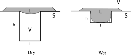
Figure 2. Dry versus Wet states

In Appendix C, a toy Markov-chain model is designed which illustrates the typical behaviors encountered in our random wetting problem. The rate of growth of the expected time to move from one stable state to the other when an unstable state lies in-between is the energy barrier between the unstable and stable states (Kramers’ law), and the random time itself normalized by its mean converges in distribution to an exponential probability distribution.

2. A simple macroscopic model. Equilibrium free energies

Before we run into similar considerations pertaining to the SOS model, let us first briefly describe some easy macroscopic arguments that led us to the forthcoming study.

2.1. No pressure $(K=0)$

DRY PHASE. Consider a well of length $l$ and height $h=\rho l.$ Call it the substrate ($S$). Fix the origin of the $\left(x,z\right)$ axis at the middle of the bottom of the well. In the following, we take $l$ as unit of length, so that the bottom of the well is the interval $\left[-0.5,+0.5\right]$ at height $z=0.$

The well is initially filled with gas or vapor ($V$). We wish to fill this groove with a liquid ($L$) in the absence of pressure ($\Delta p=\frac{K}{l}=0$). We assume that the vertical walls of the well remain dry. In a dry phase, there exists a Wulff shape separating the $LV$ phases which is pinned at $\left(x=-0.5,z=\rho\right)$ and $\left(x=0.5,z=\rho\right)$ without hitting the bottom of the well: it is the straight line joining these two corner points. The well is entirely filled with vapor, the liquid entirely stands above this straight separating line and so the liquid does not wet the substrate at all. The specific free energy of this dry phase is

(2.1) $$f_{dry}:=\frac{F_{dry}}{l}=\sigma_{LV}+\left(1+2\rho\right)\cdot\sigma_{VS},$$

where $\sigma_{AB}$ is the surface tension between the phases $A$ and $B.$

WET PHASE $(K=0)$. In a wet phase, the liquid will meet the substrate at the bottom of the well. Let $\theta$ be the Young angle between the vapor phase and the substrate at the right-most meeting point. The larger $\theta$ is, the more the substrate is hydrophilic.

Let $x_{1}\in\left(0,0.5\right)$. In a wet phase with $K=0$, the Wulff shape would indeed be made of two symmetric linear pieces of length $\frac{\rho}{\sin\theta}$, separating phase $L$ from $V$, one joining point $\left(x=-0.5,z=\rho\right)$ to point $\left(x=-x_{1},z=0\right)$ and the other joining $\left(x=x_{1},z=0\right)$ to $\left(x=0.5,z=\rho\right).$ In between, the line joining $\left(x=-x_{1},z=0\right)$ to $\left(x=x_{1},z=0\right)$ would be the flat wetting zone for the substrate. For a given $\theta$, a wet phase can exist if and only if $x_{1}>0$ or else

(2.2) $$\rho<0.5\tan\theta$$

(the well is not too deep).

When this wet phase exists, its specific free energy is

(2.3) $$f_{wet}:=\frac{F_{wet}}{l}=2\frac{\rho}{\sin\theta}\cdot\sigma_{LV}+\left(1+2\rho-2x_{1}\right)\cdot\sigma_{VS}+2x_{1}\cdot\sigma_{LS}.$$

When both phases exist, the question of which phases is favored makes sense. So we can ask for conditions under which $F_{dry}\leq F_{wet}$. Using $\sigma_{LS}-\sigma_{VS}=\sigma_{LV}\cos\theta$, we easily get the condition

(2.4) $$\rho\geq 0.5\tan\left(\theta/2\right),$$

meaning that for the dry phase to win over the wet one, the depth of the well has to be large enough.

So, when a wet phase exists ($\rho<0.5\tan\theta$), the dry phase wins over the wet phase whenever the well’s depth satisfies $\rho\geq 0.5\tan\left(\theta/2\right)$. Else, if $\rho>0.5\tan\theta$, this problem does not make sense simply because only the dry phase exists and so it necessarily wins. So, in this oversimplified wetting problem, we expect a parameter range for which the two phases wet and dry can coexist (a metastable region), and within this parameter range another parameter range for which one phase is favorable over the other. When $\rho=0.5\tan\left(\theta/2\right)$, the two phases share the same free energy (a bistable line of coexistence of both phases).

2.2. Pressure $(K>0)$

WET PHASE. The Wulff-shaped lines separating the $LV$ phases are now symmetric convex circle arcs with radius

$$r=\frac{\sigma_{LV}}{\Delta p}=l\frac{\sigma_{LV}}{K}.$$

Define the scaled radius as $R=r/l.$ In the scaled length unit and in the wet phase, we have one circle arc joining point $\left(x=-0.5,z=\rho\right)$ to point $\left(x=-x_{1},z=0\right)$ and the other joining $A:=\left(x=x_{1},z=0\right)$ to $B:=\left(x=0.5,z=\rho\right).$

Let $O$ be the center of the latter circle. Let $\varphi$ be the angle $\left(OA,OB\right).$ Then the scaled euclidean distance between $A$ and $B$ is given by (see Appendix A1)

$$AB=\left[2R^{2}\left(\sin^{2}\theta+\frac{\rho\cos\theta}{R}-\sqrt{\Delta}\right)\right]^{1/2}.$$

where $\Delta=\left(\sin^{2}\theta+\frac{\rho\cos\theta}{R}\right)^{2}-\left(\frac{\rho}{R}\right)^{2}$. Next $\widehat{AB}=2R\arcsin\left(AB/\left(2R\right)\right)$ is the scaled arc length of the arc joining $A$ to $B.$ Using

$$AB=\sqrt{\left(0.5-x_{1}\right)^{2}+\rho^{2}}.$$

gives $x_{1}$ as an explicit function of $\left(\theta,\rho,R\right)$.

For a given $\theta$, the wet phase can exist if and only if $x_{1}>0$ which is, observing $\tan\left(\theta+\varphi/2\right)=\frac{\rho}{0.5-x_{1}}$:

$$\rho<0.5\tan\left(\theta+\varphi/2\right)$$

(again, the well should not be too deep).

When this wet phase exists, its specific free energy is found to be

(2.5) $$f_{wet}:=\frac{F_{wet}}{l}=2\widehat{AB}\cdot\sigma_{LV}+\left(1+2\rho-2x_{1}\right)\cdot\sigma_{VS}+2x_{1}\cdot\sigma_{LS}+2K\cdot A_{wet},$$

where $A_{wet}=\frac{\rho}{2}\left(0.5-x_{1}\right)-\frac{1}{2}\left[R^{2}\varphi-R^{2}\sin\varphi\right]$ is the scaled dry area of the vapor beneath the right part of the Wulff shape. The right-most pressure term in (2.5) comes from

$$\frac{1}{l}\left(\Delta p\cdot l^{2}A_{wet}\right)=K\cdot A_{wet}.$$

DRY PHASE. With $\widehat{B^{\prime}B}=2R\arcsin\left(\frac{1}{2R}\right)=:R\psi,$ the arc length between the left and right corner points $B^{\prime}$ and $B$ of the well, $f_{wet}$ should be compared to the specific free energy in the dry phase which is

(2.6) $$f_{dry}:=\frac{F_{dry}}{l}=\widehat{B^{\prime}B}\cdot\sigma_{LV}+\left(1+2\rho\right)\cdot\sigma_{VS}+KA_{dry}.$$

Here $A_{dry}=\rho-\frac{1}{2}\left[R^{2}\psi-R^{2}\sin\psi\right]$ is the scaled dry area of the vapor beneath the hanging Wulff line anchored at $B^{\prime}$ and $B.$

This leads again to an implicit critical line of coexistence in the parameter space where $f_{dry}=f_{wet}.$ In Fig. 3, we plot the line of coexistence $\theta=\theta\left(K\right)$ for the arbitrary set of parameters $\sigma_{LV}=\sigma_{VS}=0.01$ and $\rho=0.2.$ The largest value of $\theta$ is obtained when $K=0$ as $\theta_{\max}=2\arctan\left(\rho/0.5\right),$ from (2.4). The largest value of $K$ is obtained from the dry phase when the circle arc pinned at the corners of the U well hits the bottom of the substrate tangentially ($\theta=0$). We get $K_{\max}=2\rho\sigma_{LV}/\left(\rho^{2}+0.5^{2}\right).$

 

Figure 3. The line of coexistence $F_{wet}=F_{dry}$ from (2.5, 2.6) with $\sigma_{LV}=\sigma_{VS}=0.01$ and $\rho=0.2$.

3. SOS model: equilibrium free energies

We now run into similar considerations for the SOS model of wetting arising in statistical mechanics. In this Section, we compute the free energies of the dry and wet phases in the thermodynamic limit for the SOS model (1.1). For the sake of simplicity, we decided to work at fixed values of the parameters $J=3.0$ and $\rho=0.2$, leaving the free parameter space be restricted to $a$ and $K$.

DRY PHASE. In the context of the SOS model (1.1), the typical Wulff shapes which come in can be described as follows. Let

$$f\left(t\right)=\left(1+J^{2}t^{2}\right)^{1/2}-1$$

with derivative

$$f^{\prime}\left(t\right)=\frac{J^{2}t}{f\left(t\right)+1}.$$

The projected interface tension $\widetilde{\sigma}_{LV}$ corresponding to (1.1) with $h_{i}\in\mathbb{R}$ and $a=0$ and boundary conditions implying a slope $\tan\theta=t$, with energy measured in units of $kT,$ is defined as

(3.1) $$\widetilde{\sigma}_{LV}\left(t\right)=\lim_{n\rightarrow\infty}-\frac{1}{n}\log Z_{n}\left(t\right):=\widetilde{\sigma}\left(t\right),$$

where

(3.2) $$\widetilde{\sigma}\left(t\right)=f\left(t\right)-\log\left(\frac{f\left(t\right)+2}{J}\right).$$

We have $\widetilde{\sigma}^{\prime}\left(t\right)=\frac{J^{2}t}{f\left(t\right)+2}.$ Then the relevant Wulff shape equations relative to (1.1) and (3.1) are implicitly given by (see [4], [8] and [9])

$$X\left(t\right)=\frac{n}{K}l_{0}\widetilde{\sigma}_{LV}^{\prime}\left(t\right);\text{ }X\left(0\right)=0$$

$$Z\left(t\right)=-\frac{n}{K}l_{0}\left(\widetilde{\sigma}_{LV}\left(t\right)-t\widetilde{\sigma}_{LV}^{\prime}\left(t\right)\right);\text{ }Z\left(0\right)=\frac{n}{K}l_{0}\log\left(\frac{2}{J}\right)$$

where $t$ is the tangent $dZ/dX$ to the curve $X\rightarrow Z\left(X\right).$

Introduce the scaled variables $x\left(t\right)=X\left(t\right)/l$ and $z\left(t\right)=Z\left(t\right)/l.$ Then, recalling $l=nl_{0}$

(3.3) $$x\left(t\right)=\frac{1}{K}\widetilde{\sigma}^{\prime}\left(t\right);\text{ }x\left(0\right)=0$$

(3.4) $$z\left(t\right)=-\frac{1}{K}\left(\widetilde{\sigma}\left(t\right)-t\widetilde{\sigma}^{\prime}\left(t\right)\right);\text{ }z\left(0\right)=\frac{1}{K}\log\left(\frac{2}{J}\right)$$

where the range of $x\left(t\right)$ is $\left(-\frac{J}{K},\frac{J}{K}\right)$ and where $t$ is the tangent $dz/dx$ to the curve $x\rightarrow z\left(x\right).$ Note that $t\left(x\right)=\frac{2Kx}{J^{2}-K^{2}x^{2}}.$

The scaled well has now unit length and fixed height $\rho=0.2.$ As before, fix the origin of the $\left(x,z\right)$ axis at the middle of the bottom of the well. We wish to derive the equation of a Wulff shape (3.3, 3.4) which is pinned at $\left(x=-0.5,z=\rho\right)$ and $\left(x=0.5,z=\rho\right)$ without hitting the bottom of the well. Let $t_{0}$ be the value of the tangent at $\left(x=0.5,z=\rho\right)$, with $t_{0}=t\left(0.5\right)=\frac{K}{J^{2}-K^{2}/4}.$ We have

$$z_{dry}\left(t\right)=z\left(t\right)-z\left(t_{0}\right)+\rho$$

so that $z_{dry}\left(0\right)=z\left(0\right)-z\left(t_{0}\right)+0.2=\frac{1}{K}\log\left(\frac{2}{J}\right)-z\left(t_{0}\right)+\rho\geq 0.$

When $K$ increases, the minimum of the hanging Wulff shape gets closer to the bottom of the well. There is a value $K=K_{\max}$ for which this minimum hits tangentially the bottom of the well in one point. The value of $K_{\max}$ is characterized by

$$z_{dry}\left(0\right)\mid_{K=K_{\max}}=\frac{1}{K_{\max}}\log\left(\frac{2}{J}\right)-z\left(\frac{K_{\max}}{J^{2}-K_{\max}^{2}/4}\right)+\rho=0.$$

The admissible range of $K$ in the dry regime is thus $\left[0,K_{\max}\right].$

In Appendix $A2a$, we obtain the specific free energy of the dry phase as 

(3.5) $$f_{dry}=K\left(0.2-z\left(t_{0}\right)\right)-2+2b\log\left[\frac{1+0.5/b}{1-0.5/b}\right].$$

Note that when $K\rightarrow 0$, $t_{0}\rightarrow 0$ and $z\left(t_{0}\right)\simeq z\left(0\right)=\frac{1}{K}\log\left(\frac{2}{J}\right).$ Thus $f_{dry}\rightarrow\log\left(\frac{J}{2}\right)=\widetilde{\sigma}\left(0\right)$ which is the specific free energy of the trivial $\left(K=0\right)-$Wulff shape joining linearly the corners of the well parallel to the bottom of the well.

WET PHASE. Let $x_{1}\in\left(0,0.5\right)$. In the wet phase, the Wulff shape is made of two symmetric convex pieces, one joining point $\left(x=-0.5,z=\rho\right)$ to point $\left(x=-x_{1},z=0\right)$ and the other joining $\left(x=x_{1},z=0\right)$ to $\left(x=0.5,z=\rho\right).$ In between, from $\left(x=-x_{1},z=0\right)$ to $\left(x=x_{1},z=0\right)$, the curve is flat, pinned to the substrate.

From [8], the specific free energy of the wet part is

(3.6) $$\sigma_{wet}=-\log\left(\frac{2a^{2}J}{2aJ-1}\right),\text{ }a\geq a_{c}:=1/J.$$

Consider the right part of the Wulff shape. Let $t_{1}$ be the tangent of the Young angle $\theta$, which is also the interface slope at $\left(x=x_{1},z=0\right)$; assuming $a\geq a_{c},$ we have (see (5)(8)(9) in [8])

(3.7) $$t_{1}=\tan\theta=\frac{2a\left(aJ-1\right)}{2aJ-1}\geq 0.$$

Note that when $a<a_{c}$, the affinity for the bottom of the well is not strong enough to produce a wet part in the equilibrium Wulff shape.

Let $t_{2}$ be the tangent of the angle of the Wulff shape at point $\left(x=0.5,z=\rho\right).$ Using the canonical equation (3.3, 3.4) of a standard Wulff shape, the equations of this Wulff shape are given by:

$$x_{wet}\left(t\right) = x\left(t\right)-x\left(t_{2}\right)+0.5$$

$$z_{wet}\left(t\right) = z\left(t\right)-z\left(t_{1}\right),$$

where $t_{2}$ has to be determined implicitly by $z_{wet}\left(t_{2}\right)=\rho.$ We then have

$$x_{1}=x_{wet}\left(t_{1}\right)=x\left(t_{1}\right)-x\left(t_{2}\right)+0.5.$$

The specific free energy of the wet phase is obtained as (see Appendix $A2b$)

(3.8) $$f_{wet}=2x_{1}\sigma_{wet}-2\left(0.5-x_{1}\right)\left(Kz\left(t_{1}\right)+2\right)+2b\log\frac{\left(1+\frac{x\left(t_{2}\right)}{b}\right)\left(1-\frac{x_{1}+x\left(t_{2}\right)-0.5}{b}\right)}{\left(1+\frac{x_{1}+x\left(t_{2}\right)-0.5}{b}\right)\left(1-\frac{x\left(t_{2}\right)}{b}\right)}.$$

When $K=0$, the two pieces of the Wulff shapes become straight lines. The tangent of the Young angle is thus $t_{1}=\rho/\left(0.5-x_{1}\right)$ and

(3.9) $$f_{wet}\mid_{K=0}=2\left(0.5-x_{1}\right)\widetilde{\sigma}\left(t_{1}\right)+2x_{1}\sigma_{wet}.$$

There exists a maximal value $a_{\max}$ of $a$ characterized by: $f_{wet}\mid_{K=0}=f_{dry}\mid_{K=0}=\log\left(J/2\right).$ For $a>a_{\max}$, the wet phase has a lower free energy than the dry phase, for all $K\geq 0$.

We fix $J=3.0$ and look for the values $a=a\left(K\right)$ for which $f_{wet}=f_{dry}$, using (3.5) and (3.8), meaning coexistence of the two phases. In this example, the range of $K$ is $\left[0,K_{\max}\right]$ with $K_{\max}\simeq 4.6767$ and the range of $a$ is $\left[a_{c},a_{\max}\right]$ with $a_{c}=1/J$ and $a_{\max}\simeq 1.5114$. Using this curve $a=a\left(K\right)$, together with (3.7), relating the Young angle $\theta$ to $a$, we rather consider the line of coexistence $\theta=\theta\left(K\right).$ This line of coexistence is shown on Fig. 4. In this phase diagram plot, the dotted lines separate a metastable region where the two phases coexist and stable regions where a single phase (either wet or dry) is stable; the solid line of coexistence separates the two stable phases within the metastable region. The two dotted lines are obtained while using $f_{sad}=f_{dry}$ and $f_{sad}=f_{wet},$ respectively. Note that the point at $K=0$ separating the dry stable zone from the metastable zone is exactly characterized by $\rho=0.2=0.5\tan\theta$ as in (2.2).

 

Figure 4. The line of coexistence $f_{dry}=f_{wet}$ from (3.5, 3.8), together with the metastability lines: $f_{dry}=f_{sad}$ from (3.5, 4.1) and $f_{wet}=f_{sad}$ from (3.8, 4.1); here $J=3.0$ and $\rho=0.2$.

4. Dynamics and numerical simulations

Let us first compute the equilibrium free energy of the saddle-point phase, characterized by a single contact point in the center of the well.

SADDLE-POINT PHASE. In the saddle-point phase, the Wulff shape is made of two symmetric pieces and $x_{1}=0$ so that there is no flat part corresponding to wetting. With $t_{1}$ the tangent of the Young angle at point $\left(x=0,z=0\right)$, the equations of the Wulff shape in the saddle-point configuration are

$$x_{sad}\left(t\right) = x\left(t\right)-x\left(t_{1}\right)$$

$$z_{sad}\left(t\right) = z\left(t\right)-z\left(t_{1}\right).$$

In Appendix $A2c$, we show that the specific free energy of the saddle phase reads

(4.1) $$f_{sad}=-Kz\left(t_{1}\right)-2+2b\log\frac{\left(1+\frac{0.5+x\left(t_{1}\right)}{b}\right)\left(1-\frac{x\left(t_{1}\right)}{b}\right)}{\left(1+\frac{x\left(t_{1}\right)}{b}\right)\left(1-\frac{0.5+x\left(t_{1}\right)}{b}\right)},$$

which is implicitly known because so is $t_{1}.$

4.1. Dynamics.

For a square well of width $l=nl_{0}$, we consider a Markovian dynamics of Monte-Carlo type having (1.1) as invariant measure. The free energy barrier to cross starting from the dry (wet) phase is $F_{sad}^{(n)}-F_{dry}^{(n)}\sim nl_{0}(f_{sad}-f_{dry})$ (respectively $F_{sad}^{(n)}-F_{wet}^{(n)}\sim nl_{0}(f_{sad}-f_{wet})$). Conventional wisdom suggests that, with $\left\langle\tau_{dw}^{\left(n\right)}\right\rangle$ the mean time needed to first enter the wet (dry) phase starting from the dry (wet) phase, in a system of size $l=nl_{0}$ as $n\to\infty$,

$$\frac{1}{nl_{0}}\log\left\langle\tau_{dw}^{\left(n\right)}\right\rangle \rightarrow f_{sad}-f_{dry}$$

$$\frac{1}{nl_{0}}\log\left\langle\tau_{wd}^{\left(n\right)}\right\rangle \rightarrow f_{sad}-f_{wet}.$$

The limiting quantities coincide, assuming coexistence, $\theta=\theta(K)$. We expect polynomial corrections such as $e^{-nl_{0}\left(f_{sad}-f_{dry}\right)}\left\langle\tau_{dw}^{\left(n\right)}\right\rangle\sim c_{dw}n^{2}$ and $e^{-nl_{0}\left(f_{sad}-f_{wet}\right)}\left\langle\tau_{wd}^{\left(n\right)}\right\rangle\sim c_{wd}n^{2}$ where $c_{dw}$ and $c_{wd}$ would be two possibly distinct $n-$independent constants. In any case, the relative weights of the dry and wet phases may differ,

(4.2) $$\lim_{n\to\infty}\frac{\left\langle\tau_{dw}^{\left(n\right)}\right\rangle}{\left\langle\tau_{dw}^{\left(n\right)}\right\rangle+\left\langle\tau_{wd}^{\left(n\right)}\right\rangle}\neq\lim_{n\to\infty}\frac{\left\langle\tau_{wd}^{\left(n\right)}\right\rangle}{\left\langle\tau_{dw}^{\left(n\right)}\right\rangle+\left\langle\tau_{wd}^{\left(n\right)}\right\rangle}\,.$$

4.2. Numerical simulation

Simulations were performed for one-dimensional interfaces over a trough of length $l=n$ and depth $h=n/5$. The interface is pinned at both ends, $h_{0}=h_{n+1}=n/5$, and $\mathbf{h}=(h_{1},\dots,h_{n})\in R_{+}^{n}$ is distributed at equilibrium according to (1.1), or

(4.3) $$\mu_{n}(d\mathbf{h})=Z_{n}^{-1}\exp(-J\sum_{i=0}^{n}|h_{i+1}-h_{i}|-\frac{K}{n}\sum_{i=1}^{n}h_{i})\prod_{i=1}^{n}(1+a\delta(h_{i}))dh_{i}$$

where the partition function $Z_{n}$ normalizes the probability.

The sub-lattice parallel heat bath dynamics, irreducible and satisfying the detailed balance condition with respect to $\mu_{n}$, is defined as follows, for $t=1,2,\dots$:

(4.4) $$P(d\mathbf{h}^{t}|\mathbf{h}^{t-1})=\mu_{n}(d\mathbf{h}^{t})\prod_{i+t\ \mathrm{odd}}\delta(h_{i}^{t}-h_{i}^{t-1})/\int\mu_{n}(d\mathbf{h})\prod_{i+t\ \mathrm{odd}}\delta(h_{i}-h_{i}^{t-1})$$

Fig. 5 shows one hundred samples obtained from this dynamics. The interface is typically near one of the two Wulff shapes, “dry” or “wet”. The parameters $J,K,a$ were chosen so that the free energies computed from the two Wulff shapes were approximately equal, so that the interface spent approximately equal times near these two shapes. The empty region between the two shapes indicates a region of small probability, which we shall call a free energy barrier.

 

Figure 5. One hundred samples of the interface for $n=700,J=3.0,K=4.0,a=0.455$ (dotted lines) and the two wulff shapes (solid lines).

The aim of the simulation is to find the law of the escape time from dry to wet or conversely. The interface can be within typical fluctuation from one of the Wulff shapes, in which case it is easy to decide whether it is “dry” or “wet”, but large deviations in between cannot be attached to one or the other in any justified way.

We measure time either in Monte-Carlo Steps per Site (MCS/S), or in Monte-Carlo Steps per Site divided by $n^{2}$ (MCS/S/$n^{2}$), because the relaxation time of a flat interface without free energy barrier is of order $n^{2}$ MCS/S in non-conservative dynamics. One MCS/S corresponds to two time steps of the form (4.4). This observation may well have interesting consequences to analyze the dynamics of spreading of nanodrops on top of rough substrates using molecular dynamics simulations.

At time intervals of the order of a few MCS/S, three measurements are taken, corresponding to the observables that make up the Hamiltonian in (4.3): the normalized length of the interface

(4.5) $$L(\mathbf{h})=\frac{1}{n+1}\sum_{i=0}^{n}|h_{i+1}-h_{i}|\,,$$

the normalized area below the interface

(4.6) $$A(\mathbf{h})=\frac{3}{n^{2}}\sum_{i=1}^{n}h_{i}\,,$$

and the number of zeroes of $\mathbf{h}$ divided by $2n$, denoted $W(\mathbf{h})$ (number of contacts with Wall). Each measurement appears as a dot on Fig. 6, making up clouds of points around the corresponding mean values for each of the two Wulff shapes. The factors of 2 and 3 in the definitions of $W(\mathbf{h})$ and $A(\mathbf{h})$ are designed to facilitate the reading in Fig. 6.

 

Figure 6. From top to bottom: $L(\mathbf{h})$, $A(\mathbf{h})$, $W(\mathbf{h})$, function of time measured in MCS/S/$n^{2}$ (dots), with $n=700,J=3.0,K=4.0,a=0.455$. The regions between 0.48 and 0.52 for $L(\mathbf{h})$, between 0.18 and 0.27 for $A(\mathbf{h})$, or between 0 and 0.04 for $W(\mathbf{h})$, correspond to the barrier between ‘dry’ and ‘wet’.

We then decide somewhat arbitrarily intervals of values of the three observables associated to the wet state or to the dry state or to the region in between, called the barrier:

$$\begin{array}[]{cccc}\mathrm{Dry:}&L(\mathbf{h})<0.48\,,&A(\mathbf{h})>0.27\,,&W(\mathbf{h})=0\\ \mathrm{Wet:}&L(\mathbf{h})>0.52\,,&A(\mathbf{h})<0.18\,,&W(\mathbf{h})>0.04\\ \mathrm{Barrier:}&\mathrm{otherwise}&&\end{array}$$

At any given time, if all three observables agree for dry, or for wet, then the interface is declared dry (D), or wet (W). Otherwise it is considered to be in the barrier (B) between dry and wet. The barrier is clearly in a region of large deviations from the dry state or from the wet state. In principle one observable should be enough, but the numerical simulation is done with a limited set of values of $n$, and the picture emerges more clearly using three observables.

We thus obtain a marginal of the interface dynamics, which is a non-Markovian process with values in {D,B,W}. Of course the simulation uses discrete time, but the mean sojourn time in D or B or W is of order $n^{2}$ MCS/S, so that a continuous time description is better, with numerical results expressed in MCS/S/$n^{2}$.

A marginal of this marginal is the sequence of letters, forgetting their duration, looking like

DBDBDBDBWBWBWBWBWBWBWBWBDBDBDBDBDBWBWB…

with only four 2-letter patterns: DB, BD, WB, BW. This restriction allows only six 3-letter patterns: DBD, BDB, WBW, BWB, DBW, WBD. The last two are very rare ($\sim\exp(-\mathrm{const.}n)$). The numerical algorithm does not strictly forbid the 2-letter patterns DW or WD, crossing the barrier in a few MCS/S, but they are so rare, with a relative frequency expected $\sim\exp(-\mathrm{const.}n^{2})$, that we haven’t seen them in the experiment.

The limiting relative frequencies of the letters D, B, W, are respectively 1/4, 1/2, 1/4. The barrier B should be decomposed into a dry side and a wet side of the saddle point. We cannot describe precisely the corresponding configurations, but we can assume that within a 3-letter pattern DBD, the system remains in the dry state, or on the dry side of the saddle point, and analogously for WBW. If we would change every B in DBD into D, and every B in WBW into W, then we would find relative frequencies tending to 1/2, 1/2 for D and W. The corresponding partition of the configuration space into D and W is analogous to partitions which play a role in some studies of metastability [7]. There is of course a remainder $\sim\exp(-\mathrm{const.}n)$ for B from DBW and WBD.

The dynamics is started at time $t_{0}=0$ in D, with the interface near the Wulff shape associated with the dry state. The first time in W is denoted $t_{1}$, measured in MCS/S/$n^{2}$. The next time in D is denoted $t_{2}$, etc. Thus $t_{2k+1}$ is the first time in W after $t_{2k}$ for $k=0,1,\dots,k_{\max}$ and $t_{2k}$ is the first time in D after $t_{2k-1}$ for $k=1,2,\dots,k_{\max}$. We also define $t_{2k}^{\prime}$ as the last time in D before $t_{2k+1}$ and after $t_{2k}$, and $t_{2k+1}^{\prime}$ as the last time in W before $t_{2k+2}$ and after $t_{2k+1}$. The empirical mean escape times from D and from W are defined respectively as

(4.7) $$\bar{\tau}_{D}=\frac{1}{k_{\max}}\sum_{k=0}^{k_{\max}-1}(t_{2k}^{\prime}-t_{2k})\,,\text{ }\bar{\tau}_{W}=\frac{1}{k_{\max}}\sum_{k=0}^{k_{\max}-1}(t_{2k+1}^{\prime}-t_{2k+1})$$

and the empirical mean barrier crossing time is defined as

(4.8) $$\bar{\tau}_{B}=\frac{1}{2k_{\max}}\sum_{\ell=0}^{2k_{\max}-1}(t_{\ell+1}-t_{\ell}^{\prime})$$

The total time of the experiment is $k_{\max}(\bar{\tau}_{D}+\bar{\tau}_{W})+2k_{\max}\bar{\tau}_{B}$, in MCS/S/$n^{2}$. The measured escape times from D and from W are respectively $\tau_{k}^{D}=t_{2k}^{\prime}-t_{2k}$ and $\tau_{k}^{W}=t_{2k+1}^{\prime}-t_{2k+1}$. They are not a priori independent nor identically distributed, but one may study the empirical cumulative distribution function of a random variable $\tau^{D}$ or $\tau^{W}$ having the sequence of realizations $\tau_{k}^{D}$ or $\tau_{k}^{W}$:

(4.9) $$R^{D}(t)=\frac{1}{k_{\max}}|\{k:\tau_{k}^{D}\leq t\}|\,,\qquad R^{W}(t)=\frac{1}{k_{\max}}|\{k:\tau_{k}^{W}\leq t\}|$$

Figure 7. Empirical cumulative distribution function of $\tau_{k}^{D}$ (dry) and $\tau_{k}^{W}$ (wet) and fit $R^{D}(t)=1-\exp(-(t+1.2)/27.8)$, $R^{W}(t)=1-\exp(-(t+1.3)/27.5)$, functions of time in MCS/S/$n^{2}$, for $n=500,J=3.0,K=4.0,a=0.451$, and $k_{\max}=93$.

This is shown on Fig. 7, showing that $\tau^{D}$ and $\tau^{W}$ are approximately independent and identically distributed (iid) exponential random variables. The fit is better with a small shift as indicated, which we interpret as a redistribution of the barrier time $2k_{\max}\bar{\tau}_{B}$ to the dry and wet states, in a proportion which we cannot decide directly.

Figure 8. $\log(\bar{\tau}^{D})/n$ (dry) and $\log(\bar{\tau}^{W})/n$ (wet) and fit $c+d*\log(n)/n$ for $J=3.0,K=4.0$, and $a=0.4375,\,0.445,\,0.449,\,0.451,\,0.453,\,0.455,\,0.456$ for $n=200,300,400,500,600,700,800$ respectively.

We now turn to the dependence of $\bar{\tau}^{B}$, $\bar{\tau}^{D}$ and $\bar{\tau}^{W}$ upon $n$. Fig. 8 shows that $\log(\bar{\tau}^{D})/n$ and $\log(\bar{\tau}^{W})/n$ tend to a constant $\simeq 0.0105$ as $n\to\infty$, to be compared with the free energy density difference between the barrier or saddle point and the dry or wet states, giving a theoretical value $0.0129$, cf. (4.1)(3.5)(3.8). On the other hand $\bar{\tau}^{B}$, measured like the other times in MCS/S/$n^{2}$ appears to converge to a limit independent of $n$, $\bar{\tau}^{B}=0.22\pm 0.03$ for $n=500,600,700,800$.

For each value of $n$, the simulations were done with a value $a_{n}$ of the parameter $a$ chosen so that the system spent equal time in ‘dry’ and in ‘wet’. Finite size corrections to the thermodynamic limit should imply $a_{n}=a+O(1/n)$; a fit by $a_{n}=a_{\infty}+\mathrm{const.}/n$ gives $a_{\infty}=4.61$, with an uncertainty compatible with the expected limit $a\simeq 4.64$, as can be read on Fig. 4 at $K=4.0$.

The size of samples used in Fig. 8 for $n=200,300,400,500,600,700,800$ was $k_{\max}=15702,4936,2433,778,272,47,19$ respectively, where $k_{\max}$ is the number of observed transitions from ‘dry’ to ‘wet’, also equal to the number of observed transitions from ‘wet’ to ‘dry’.

5. Conclusion

We describe a situation where a liquid droplet is on top of a structured substrate presenting grooves or wells. We show that there exists a range of parameters for which wetting and non-wetting states both share the same free energy, entailing that there can be transitions between these two states. We calculate analytically the involved free energies of the dry and wet states in the context first of a simple thermodynamical model and then for a random microscopic model based on the Solid-on-Solid (SOS) model. In the latter case, we present a dynamical model showing stochastic transitions between the wetting and non-wetting states. We show that the expected time to switch from one state to the other grows exponentially with the free energy barrier between the stable states and the saddle state, proportional to the width of the grooves. This random time is shown to have an exponential-like distribution. Our study hopefully contributes to a better comprehension of the behavior of fluids on structured surfaces.

6. Appendix

A1. Proof of (2.5).

Let $O$ be the center of the circle anchored at $A$ and $B$ with scaled radius $R$. With $\varphi$ the angle $\left(OA,OB\right),$ the scaled euclidean distance between $A$ and $B$ is

$$AB=2R\sin\left(\frac{\varphi}{2}\right)=\sqrt{\left(0.5-x_{1}\right)^{2}+\rho^{2}}.$$

The scaled arc length of the arc joining $A$ to $B$ is thus

$$\widehat{AB}=R\varphi=2R\arcsin\left(\frac{\sqrt{\left(0.5-x_{1}\right)^{2}+\rho^{2}}}{2R}\right).$$

Using $\sin\left(\theta+\varphi/2\right)=\frac{\rho}{AB}$ and $AB=2R\sin\left(\frac{\varphi}{2}\right)$ gives $AB,$ after eliminating $\varphi.$ With $\Delta=\left(\sin^{2}\theta+\frac{\rho\cos\theta}{R}\right)^{2}-\left(\frac{\rho}{R}\right)^{2},$ we get $AB$ as the explicit function of $\left(\theta,\rho,R\right):$

$$AB^{2}=2R^{2}\left(\sin^{2}\theta+\frac{\rho\cos\theta}{R}-\sqrt{\Delta}\right).$$

Note that, geometrically, $\rho<R\cos\theta$ which entails that $\Delta>0.$

As a result, $\widehat{AB}=2R\arcsin\left(AB/\left(2R\right)\right),$ $x_{1}=0.5-\sqrt{AB^{2}-\rho^{2}}$ and $\varphi=2\arcsin\left(AB/\left(2R\right)\right)$ have themselves an explicit expression in terms of $\left(\theta,\rho,R\right)$. These quantities are the ones needed to compute $f_{wet}$ from (2.5).

A2. Proofs of (3.5), (3.8) and (4.1).

$A2a$ (DRY PHASE). The specific free energy $f_{dry}\left(x_{1},x_{2}\right):=\lim_{l\rightarrow\infty}\frac{F_{dry}\left(x_{1},x_{2}\right)}{l}$ of the dry phase between $\left(x_{1},x_{2}\right)$ has two contributions, one pertaining to the length and the other to the area below the interface, namely:

(6.1) $$f_{dry}\left(x_{1},x_{2}\right)=\int_{x_{1}}^{x_{2}}\widetilde{\sigma}dx+K\int_{x_{1}}^{x_{2}}z_{dry}dx=\int_{x_{1}}^{x_{2}}t\widetilde{\sigma}^{\prime}dx+K\left(x_{2}-x_{1}\right)\left(0.2-z\left(t_{0}\right)\right).$$

With $b:=J/K,$ we have

$$\int_{x_{1}}^{x_{2}}t\widetilde{\sigma}^{\prime}dx=K\int_{x_{1}}^{x_{2}}txdx=\int_{x_{1}}^{x_{2}}\frac{2K^{2}x^{2}}{J^{2}-K^{2}x^{2}}dx=2\int_{x_{1}}^{x_{2}}\frac{x^{2}/b^{2}}{1-x^{2}/b^{2}}dx$$

$$=-2\left(x_{2}-x_{1}\right)+\int_{x_{1}}^{x_{2}}\left(\frac{1}{1-x/b}+\frac{1}{1+x/b}\right)dx$$

$$=-2\left(x_{2}-x_{1}\right)+b\log\left[\frac{1+x_{2}/b}{1+x_{1}/b}\frac{1-x_{1}/b}{1-x_{2}/b}\right].$$

Finally, letting $x_{1}=-0.5,x_{2}=0.5$, we obtain the specific free energy of the dry phase as in (3.5).

$A2b$ (WET PHASE). The limiting specific free energy of the wet phase has two parts, one corresponding to the symmetric pieces of the Wulff shape, the other to the flat part:

(6.2) $$f_{wet}=2\int_{x_{1}}^{0.5}\left(\widetilde{\sigma}+Kz_{wet}\right)dx_{wet}+2x_{1}\sigma_{wet}.$$

We have

$$\int_{x_{1}}^{x_{2}}\left(\widetilde{\sigma}+Kz_{wet}\right)dx_{wet}=-Kz\left(t_{1}\right)\left(x_{2}-x_{1}\right)+\int_{x_{1}+x\left(t_{2}\right)-0.5}^{x_{2}+x\left(t_{2}\right)-0.5}\left(\widetilde{\sigma}+Kz\right)dx$$

and, using

$$\int_{\alpha}^{\beta}\left(\widetilde{\sigma}+Kz\right)dx=\int_{\alpha}^{\beta}t\widetilde{\sigma}^{\prime}dx=-2\left(\beta-\alpha\right)+b\log\frac{\left(1+\frac{\beta}{b}\right)\left(1-\frac{\alpha}{b}\right)}{\left(1+\frac{\alpha}{b}\right)\left(1-\frac{\beta}{b}\right)},$$

we finally obtain

$$f_{wet}=2x_{1}\sigma_{wet}-2Kz\left(t_{1}\right)\left(0.5-x_{1}\right)+2\int_{x_{1}+x\left(t_{2}\right)-0.5}^{x\left(t_{2}\right)}\left(\widetilde{\sigma}+Kz\right)dx,$$

leading to (3.8).

$A2c$ (SADDLE PHASE). The slope $t_{2}$ of the interface at point $\left(x=0.5,z=\rho\right)$ has to be determined implicitly by $z_{sad}\left(t_{2}\right)=\rho.$ We have

$$x_{sad}\left(t_{2}\right)=x\left(t_{2}\right)-x\left(t_{1}\right)=0.5$$

$$z_{sad}\left(t_{2}\right)=z\left(t_{2}\right)-z\left(t_{1}\right)=\rho.$$

From the first equation, recalling $x\left(t\right)=\frac{1}{K}$ $\widetilde{\sigma}^{\prime}\left(t\right)$ and $\widetilde{\sigma}^{\prime}\left(t\right)=\frac{J^{2}t}{f\left(t\right)+2}=\frac{J^{2}t}{\left(1+J^{2}t^{2}\right)^{1/2}+1}$

$$t_{2}=\widetilde{\sigma}^{\prime-1}\left(\widetilde{\sigma}^{\prime}\left(t_{1}\right)+0.5K\right)=:\varphi\left(t_{1}\right)$$

where the inverse of $\widetilde{\sigma}^{\prime}$ is easily seen to be

$$\widetilde{\sigma}^{\prime-1}\left(s\right)=\frac{2s}{J^{2}-s^{2}}.$$

Thus $t_{2}=\varphi\left(t_{1}\right)$ is an explicit known function of $t_{1}.$ Plugging this expression in the second equation and recalling $z\left(t\right)=-\left(\widetilde{\sigma}\left(t\right)-t\widetilde{\sigma}^{\prime}\left(t\right)\right)/K$,

$$\left(\widetilde{\sigma}-t\widetilde{\sigma}^{\prime}\right)\left(\varphi\left(t_{1}\right)\right)-\left(\widetilde{\sigma}-t\widetilde{\sigma}^{\prime}\right)\left(t_{1}\right)=-\rho K$$

giving $t_{1}$ implicitly and then $t_{2}$ using $t_{2}=\varphi\left(t_{1}\right)$. The specific free energy of the saddle-point phase is thus

(6.3) $$f_{sad}=2\int_{0}^{0.5}\left(\widetilde{\sigma}+Kz_{sad}\right)dx_{sad}.$$

We have

$$\int_{x_{1}}^{x_{2}}\left(\widetilde{\sigma}+Kz_{sad}\right)dx_{sad}=-Kz\left(t_{1}\right)\left(x_{2}-x_{1}\right)+\int_{x_{1}+x\left(t_{1}\right)}^{x_{2}+x\left(t_{1}\right)}\left(\widetilde{\sigma}+Kz\right)dx$$

and so

$$f_{sad}=-Kz\left(t_{1}\right)+2\int_{x\left(t_{1}\right)}^{0.5+x\left(t_{1}\right)}\left(\widetilde{\sigma}+Kz\right)dx,$$

leading to (4.1).

B. A toy model.

Although the problems encountered in this study are far from being Markovian, we find it useful to end up with recalling similar issues in the context of Markov chains or the like.

Consider a discrete-time $k$ Markov chain $X_{k}$ with five states $\left\{0,1,2,3,4\right\}.$ Suppose the following transition probabilities $P_{i,j}$ from state $i$ to $j$ hold: $P_{0,0}=1-\alpha^{\prime}$, $P_{0,1}=\alpha^{\prime}$; $P_{1,0}=1-\alpha$, $P_{1,2}=\alpha$; $P_{2,1}=1/2$, $P_{2,3}=1/2$; $P_{3,2}=\alpha$, $P_{3,4}=1-\alpha$; $P_{4,3}=\alpha^{\prime}$, $P_{4,4}=1-\alpha^{\prime}.$

The parameters $\alpha$ and $\alpha^{\prime}$ are small, with

$$\alpha = e^{-\left[U\left(2\right)-U\left(3\right)\right]/\varepsilon}=e^{-\left[U\left(2\right)-U\left(1\right)\right]/\varepsilon}$$

$$\alpha^{\prime} = e^{-\left[U\left(3\right)-U\left(4\right)\right]/\varepsilon}=e^{-\left[U\left(1\right)-U\left(0\right)\right]/\varepsilon},$$

the energy barrier terms within the brackets being all positive and $\varepsilon$ small. Thus $\left\{0\right\}$ and $\left\{4\right\}$ are two stable states separated by a barrier state $\left\{2\right\}$. Let us compute the law of the time $\tau_{0,4}=\inf\left(k:X_{k}=4\mid X_{0}=0\right)$ needed to move from state $\left\{0\right\}$ to state $\left\{4\right\}.$ The chain is a nearest neighbors birth and death chain which is ergodic. Putting $p_{x}=P_{x,x+1}$ and $q_{x}=P_{x,x-1}$, the invariant measure is $\pi_{x}=\pi_{0}\prod_{y=0}^{x-1}\frac{p_{y}}{q_{y+1}}$. Starting from $\left\{0\right\}$, the sample paths are made of iid excursions separating consecutive visits to $\left\{0\right\}.$ The law of the height $H$ of an excursion is given by

$$\Pr\left(H\geq h\right)=\frac{1}{\varphi\left(h\right)},$$

where

$$\varphi\left(x\right)=1+\sum_{y=1}^{x-1}\prod_{z=1}^{y}\frac{q_{z}}{p_{z}}$$

is the scale function of the chain. In particular, we get $\Pr\left(H=4\right)=1/\varphi\left(4\right)=\alpha/2.$

With $\mu$ the mean length of an excursion and $H_{i}$ the height of excursion $i$, we have

$$\Pr\left(\tau_{0,4}>K\right)=\Pr\left(\sup_{k\leq K}X_{k}<4\right)\approx\Pr\left(\max_{i=1,..,\left[K/\mu\right]}H_{i}<4\right)=\Pr\left(H_{1}<4\right)^{\left[K/\mu\right]}.$$

Thus $\Pr\left(\tau_{0,4}>K\right)\approx\left(1-\Pr\left(H_{1}=4\right)\right)^{\left[K/\mu\right]}$. Observing that $\mu$ is of order $1/\alpha^{\prime}$, we get that the mean value of $\tau_{0,4}$ is of order $1/\left(\alpha\alpha^{\prime}\right)=e^{\left[U\left(2\right)-U\left(0\right)\right]/\varepsilon}$ with

(6.4) $$\Pr\left(\alpha\alpha^{\prime}\tau_{0,4}>t\right)\rightarrow e^{-t/2}\text{ as }\varepsilon\text{ gets small}.$$

Thus the expected mean time to move from $\left\{0\right\}$ to $\left\{4\right\}$ is the exponential of the global energy barrier $U\left(2\right)-U\left(0\right)$ normalized by $\varepsilon$ and the time $\tau_{0,4}$ normalized by its mean converges in distribution to an exponential distribution with mean $2$.

We can check that in the latter model $\pi_{0}+\pi_{1}=\pi_{3}+\pi_{4}$ showing that the two stable state basins share the same weight.

Suppose the states $\left\{0\right\}$ $\left\{2\right\}$ $\left\{4\right\}$ have a width, say $L_{0},$ $L_{2}$ and $L_{4},$ where the Markov chain undergoes a symmetric random walk before possibly attempting to overcome the energy barrier. In this case, the mean values are expected to behave like

$$\left\langle\tau_{0,4}\right\rangle \simeq L_{0}L_{2}e^{\left(U\left(2\right)-U\left(0\right)\right)/\varepsilon}$$

$$\left\langle\tau_{4,0}\right\rangle \simeq L_{4}L_{2}e^{\left(U\left(2\right)-U\left(4\right)\right)/\varepsilon}$$

including a factor involving the characteristic plateaux lengths of the steady states. The walker has to overcome its energy barrier but also spends some time in the flat regions $\left\{0,2\right\}$ for the move $\left\{0\right\}\rightarrow\left\{4\right\}$ and $\left\{2,4\right\}$ for the move $\left\{4\right\}\rightarrow\left\{0\right\}.$ The condition $L_{0}\neq L_{4}$ introduces some skewness in the equilibrium weights of the two stable state basins. These considerations are the discrete space-time versions of the result known for a Langevin-type stochastic differential equation evolving in a quartic double-well potential $U$ with additive white noise with small local variance $\varepsilon.$ In this context, [11], if $a$ and $b$ are the stable states corresponding to a global minimum of $U$ and if $c$ is the in-between unstable state

$$\left\langle\tau_{a,b}\right\rangle \simeq \frac{1}{\sqrt{U^{\prime\prime}\left(a\right)\left|U^{\prime\prime}\left(c\right)\right|}}e^{\left(U\left(c\right)-U\left(a\right)\right)/\varepsilon}$$

$$\left\langle\tau_{b,a}\right\rangle \simeq \frac{1}{\sqrt{U^{\prime\prime}\left(b\right)\left|U^{\prime\prime}\left(c\right)\right|}}e^{\left(U\left(c\right)-U\left(b\right)\right)/\varepsilon}.$$

Coming back to the previous symmetric case where $\left\{0\right\}$ $\left\{2\right\}$ $\left\{4\right\}$ are ‘simple’ states, we finally address the following problem: what is the time $\widetilde{\tau}_{0,4}$ needed to first hit state $\left\{4\right\}$ starting from $\left\{0\right\}$ given the walker does not return to $\left\{0\right\}$ again. Note that

$$\widetilde{\tau}_{0,4}=\tau_{0,4}-\sup\left(k<\tau_{0,4}:X_{k}=0\mid X_{0}=0\right).$$

We have $\widetilde{\tau}_{0,4}=1+\tau_{1,4}$ where $\tau_{1,4}$ is the time needed to first hit state $\left\{4\right\}$ starting from $\left\{1\right\}$ of the ergodic chain governed by the transition matrix on $\left\{1,..,4\right\}^{2}$: $Q_{1,1}=0$, $Q_{1,2}=1$; $Q_{2,1}=1/2$, $Q_{2,3}=1/2$; $Q_{3,2}=\alpha$, $Q_{3,4}=1-\alpha$; $Q_{4,3}=\alpha^{\prime}$, $Q_{4,4}=1-\alpha^{\prime}.$ For this $Q-$chain, the state $\left\{1\right\}$ is now purely reflecting. Using the scale function $\varphi$ of this new chain, $\Pr\left(H=4\right)=1/\varphi\left(4\right)=\frac{1-\alpha}{2+\alpha}\rightarrow 1/2$ ($\varepsilon\rightarrow 0$). Similarly, the mean return time $\mu$ to state $\left\{1\right\}$ tends to a finite value when $\varepsilon\rightarrow 0$ so that the mean value of $\widetilde{\tau}_{0,4}$ tends itself to a finite value when $\varepsilon\rightarrow 0$. Given there is no possible return to state $\left\{0\right\}$, the mean time to first hit state $\left\{4\right\}$ turns out to be very short compared to $\tau_{0,4}$ itself.

References

- [1] D. B. Abraham, E. R. Smith, Surface-film thickening: An exactly solvable model. Phys. Rev. B, 26, No 3, 1480-1482, 1982.
- [2] D. B. Abraham, J. de Coninck, Description of phases in a film-thickening transition. J. Phys. A, 16, L333-L337, 1983.
- [3] D. B. Abraham, E. R. Smith, An exactly solved model with a wetting transition, J. Stat. Phys., 43, No 3/4, 621-643, 1986.
- [4] H. van Beijeren, I. Nolden: pp 259–300 in Structure and Dynamics of Surfaces II, edited by W. Schommers and P. von Blanckenhagen. Topics in Current Physics Vol. 43 (Springer-Verlag, Berlin Heidelberg, 1987).
- [5] Bormashenko E., Pogreb R., Whyman G. Erlich M. Cassie-wenzel wetting transition in vibrating drops deposited on rough surfaces: Is the dynamic Cassie-Wenzel wetting transition a 2D or 1D affair? Langmuir 23, 4999-5003, 2010.
- [6] Bo He, N. A. Patankar, J. Lee, Multiple equilibrium droplet shapes and design criterion for rough hydrophobic surfaces. Langmuir 19, 4999-5003, 2003.
- [7] A. Bovier, M. Eckhoff, V. Gayrard, M. Klein: Metastability and small eigenvalues in Markov chains, J. Phys. A: Math. Gen., 33, L447–L451 (2000).
- [8] J. de Coninck, F. Dunlop, Wetting transitions and contact angles, Europhys. Lett., 4, No 11, 1291-1296, 1987.
- [9] J. de Coninck, F. Dunlop, T. Huillet, A necklace of Wulff shapes. J. Stat. Phys., 123, No 1, 223-236, 2006.
- [10] M. Gross, F. Varnik, D. Raabe, I. Steinbach, Small droplets on superhydrophobic surfaces. Phys. Rev. E. 81, 051606, 2010.
- [11] N. G. van Kampen, Stochastic processes in physics and chemistry. Lecture Notes in Mathematics, 888. North-Holland Publishing Co., Amsterdam-New York, 1981.