Dynamics and kinetics of quasiparticle decay in a nearly-one-dimensional degenerate Bose gas

Abstract

We consider decay of a quasiparticle in a nearly-one-dimensional quasicondensate of trapped atoms, where virtual excitations of transverse modes break down one-dimensionality and integrability, giving rise to effective three-body elastic collisions. We calculate the matrix element for the process that involves one incoming quasiparticle and three outgoing quasiparticles. Scattering that involves low-frequency modes with high thermal population results in a diffusive dynamics of a bunch of quasiparticles created in the system.

I Introduction

An uniform one-dimensional (1D) system of indistinguishable bosons interacting with each other via pairwise delta-functional potential is known to be integrable and described by the Lieb-Liniger model LL . In an integrable system, the number of integrals of motion equals to the number of degrees of freedom. Such an equality, on the one hand, facilitates analytical treatment of integrable models and, on the other hand, make their dynamics quite distinct from the dynamics of non-integrable many-body systems. In the course of its evolution, an integrable system always “remembers” the information on its initial conditions, and relaxation to a thermal equilibrium state does not occur. A general review of integrable models can be found, e.g., in Ref. Thacker . The Lieb-Liniger model can be implemented in an ultracold-atom experiment in optical lattices je1 or on atom chips je2 . The conditions of the 1D regime require both the temperature and mean interaction energy per atom being well below the excitation quantum $\hbar\omega_{\perp}$ of the radial trapping (harmonic oscillator) Hamiltonian:

$$T\lesssim\hbar\omega_{\perp},\qquad g_{\mathrm{1D}}n_{\mathrm{1D}}\lesssim\hbar\omega_{\perp}.$$ (1)

Here temperature $T$ is measured in units of energy (i.e., we set $k_{\mathrm{B}}=1$) and $n_{\mathrm{1D}}$ is the linear density of atoms. Since the effective 1D interaction strength for atoms under radial harmonic confinement is (far below the confinement-induced resonance Olsh ) $g_{\mathrm{1D}}=2\hbar\omega_{\perp}a_{s}$, where $a_{s}$ is the atomic $s$-wave scattering length Under these conditions explsm , the latter of two Eqs. (1) reads

$$n_{\mathrm{1D}}a_{s}\lesssim 1.$$ (2)

If Eqs. (1) hold then radial motion of atoms is confined to the ground state of the radial trapping Hamiltonian. Ultracold atomic systems in the 1D regime can be prepared in optical lattices WeissNC and on atom chips Ho1 . However, in reality no system is perfectly 1D, but the actual question is, on which timescale it can be described as 1D. Since the thermal population of the excited states is strongly suppressed by the exponential Boltzmannian factor, already $T\approx 0.2\,\hbar\omega_{\perp}$ Ho1 corresponds to a deeply 1D regime in terms of thermal excitations. On the other hand, the influence of atomic interactions is a more complicated and interesting issue. For ultracold atoms under tight lateral confinement one-dimensionality and, hence, integrability are lifted by atomic interactions causing virtual population of excited radial modes. The role of the virtual radial excitations in the dynamics of ultracold atomic gases in tight waveguides has been first studied in the context of macroscopic flow of degenerate atomic gas through a waveguide SPR and decay Muryshev or inelastic collisions Malomed of mean-field solitons. On the microscopic level, a second-order perturbative collisional process with a radially excited virtual (intermediate) state give rises to effective three-body elastic scattering that has been suggested as the source of thermalization in ultracold atomic gases on atom chips Mazets1 ; Mazets2 .

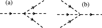
Figure 1: Feynman diagrams of the processes studied in the present paper: (a) splitting of an elementary excitation into three excitations, (b) the reciprocal process.

Damping of a fast particle motion in a quasi-1D bosonic system due to the effective three-body process shown in Fig. 1 has been studied recently Glazman , and the contribution of events with small momentum transfer to the damping rate has been found significant in a certain parameter range. The reason is the bosonic amplification of scattering into modes with high thermal population Glazman . In the present paper we derive (i) the vertex for the diagrams in Fig. 1 and (ii) a kinetic equation describing damping relaxation of a quasiparticle in a degenerate nearly-1D bosonic system and its diffusion-type limit describing the elementary excittation dynamics induced by collisions with a small momentum transfer.

Using our theoretical estimations, we conclude that the three-body elastic processes responsible for the integrability breakdown can be detected experimentally by observing the damping dynamics of an ensemble of fast particles on relatively short time scales.

II Physical model

The Hamiltonian of a 1D system of identical bosons with an additional term accounting for effective three-body interactions via virtual radial excitations reads

$$\hat{H}=\hat{H}_{\mathrm{LL}}+\hat{H}_{\mathrm{3b}},$$ (3)

where $\hat{H}_{\mathrm{LL}}$ is the Hamiltonian of the Lieb-Liniger model written in terms of the 1D number density $\hat{n}$ and phase $\hat{\phi}$ operators Popov ; MC

$$\hat{H}_{\mathrm{LL}}=\int_{0}^{L}dz\,{\bigg{[}}\frac{\hbar^{2}}{2m}\frac{\partial\hat{\phi}}{\partial z}\hat{n}\frac{\partial\hat{\phi}}{\partial z}+\frac{\hbar^{2}}{8m}\hat{n}^{-1}\left(\frac{\partial\hat{n}}{\partial z}\right)^{2}+\frac{g_{\mathrm{1D}}}{2}\hat{n}^{2}{\bigg{]}},$$ (4)

where $m$ is the atomic mass and $L$ is the quantization length. The commutation rule for the phase and density operators is $[\phi(z),n(z^{\prime})]=-i\delta(z-z^{\prime})$. The three-body collisional dynamics is taken into account by the term

$$\hat{H}_{\mathrm{3b}}=-\frac{\xi}{2}\hbar\omega_{\perp}a_{s}^{2}\int_{0}^{L}dz\,\hat{n}^{3},$$ (5)

where $\xi=4\ln\frac{4}{3}$. Note that an error in the prefactor of $\hat{H}_{\mathrm{ni}}$ Mazets1 has been corrected later Mazets2 ; Glazman . Of course, Eq. (5) is only a lowest term in expansion of the integrability-breaking interaction in powers of the small parameter $n_{\mathrm{1D}}a_{s}$. The full effective interaction due to excitation of radial modes contains cubic, quartic, quintic in $\hat{n}$ terms and supports a stable ground state. This can be seen from the analogy with the mean-field variational approach SPR ; Mazets2 . However, if Eq. (2) holds then Eq. (5) is sufficient for perturbative calculation of the rates of the processes shown schematically in Fig. 1.

From now on, we scale energy to $g_{\mathrm{1D}}n_{\mathrm{1D}}$ and set the healing length $\zeta_{\mathrm{h}}=\hbar/\sqrt{mg_{\mathrm{1D}}n_{\mathrm{1D}}}$ as the length unit, i.e., $\hat{H}\equiv g_{\mathrm{1D}}n_{\mathrm{1D}}\hat{\bar{H}}$ and $z=\zeta_{\mathrm{h}}\bar{z}$. In what follows, we omit, for the sake of compactness of notation, the bar over scaled values. It will not lead to confusion, since we will mention explicitly the return to usual units. In the new, dimensionless form Eqs. (4, 5) read simply as

$$\hat{H}_{\mathrm{LL}}=\int_{0}^{L}dz\,{\bigg{[}}\frac{1}{2}\frac{\partial\hat{\phi}}{\partial z}\hat{n}\frac{\partial\hat{\phi}}{\partial z}+\frac{1}{8}\hat{n}^{-1}\left(\frac{\partial\hat{n}}{\partial z}\right)^{2}+\frac{1}{2n_{\mathrm{1D}}}\hat{n}^{2}{\bigg{]}},$$ (6)

$$\hat{H}_{\mathrm{ni}}=-\frac{\kappa_{\mathrm{3b}}}{n_{\mathrm{1D}}^{2}}\int_{0}^{L}dz\,\hat{n}^{3},$$ (7)

where $\kappa_{\mathrm{3b}}=\frac{1}{4}\xi n_{\mathrm{1D}}a_{s}$.

We expand the phase and density operators in plane waves. The average 1D density $n_{\mathrm{1D}}=N/L$ is an integral of motion has a well-defined value since the total number $N$ of atoms is fixed. The expansions read as

$$\hat{n}=n_{\mathrm{1D}}+\sum_{k}\hat{n}_{k}\frac{e^{ikz}}{\sqrt{L}},\quad\hat{\phi}=\Phi_{0}+\sum_{k}\hat{\phi}_{k}\frac{e^{ikz}}{\sqrt{L}}.$$ (8)

The global phase $\Phi_{0}$, subject to phase diffusion even if $N=$ const Lewenstein , will not appear in further expressions. The sums in Eq. (8) are taken of non-zero (both positive and negative) integer multiples of $2\pi/L$. The commutation rule for the phase and density operators in the momentum representation are

$$[\hat{\phi}_{k},\hat{n}_{-k^{\prime}}]=-i\delta_{kk^{\prime}}.$$ (9)

By re-grouping terms we express the full Hamiltonian of the system as $\hat{H}=E_{\mathrm{gr}}+\hat{H}_{\mathrm{h}}+\hat{H}_{\mathrm{a}}+\hat{H}_{\mathrm{ni}}$, where $E_{\mathrm{gr}}$ is the ground state energy, the two next terms represent the harmonic

$$\hat{H}_{\mathrm{h}}=\sum_{k}\left[\frac{n_{\mathrm{1D}}k^{2}}{2}\hat{\phi}_{k}\hat{\phi}_{-k}+\left(\frac{k^{2}}{8n_{\mathrm{1D}}}+\frac{G_{\mathrm{rn}}}{2n_{\mathrm{1D}}}\right)\hat{n}_{k}\hat{n}_{-k}\right]$$ (10)

and anharmonic

$$\hat{H}_{\mathrm{a}}=\frac{1}{\sqrt{L}}\sum_{q,q^{\prime}}\frac{qq^{\prime}}{2}\left(-\hat{\phi}_{q}\hat{n}_{-q-q^{\prime}}\hat{\phi}_{q^{\prime}}+\frac{1}{4n_{\mathrm{1D}}^{2}}\hat{\nu}_{-q-q^{\prime}}\hat{n}_{q}\hat{n}_{q^{\prime}}\right)$$ (11)

parts of the Lieb-Liniger model Hamiltonian. Operator $\hat{\nu}_{k}$ in Eq. (11) is defined as

$$\hat{\nu}_{k} = \frac{n_{\mathrm{1D}}}{\sqrt{L}}\int_{0}^{L}dz\,e^{-ikz}\left(n_{\mathrm{1D}}^{-1}-\hat{n}^{-1}\right)$$ (12)

$$= \hat{n}_{k}-\frac{1}{\sqrt{L}n_{\mathrm{1D}}}\sum_{k^{\prime}}\hat{n}_{k-k^{\prime}}\hat{n}_{k^{\prime}}+\dots~{}.$$

$G_{\mathrm{rn}}=1-\frac{3}{4}\xi n_{\mathrm{1D}}a_{s}$ in Eq. (10) is the effective strength of pairwise interactions renormalized by the presence of the three-body collisions. In usual units, the coupling strength $g_{\mathrm{1D}}$ renormalizes to $g_{\mathrm{1D}}^{\prime}=Gg_{\mathrm{1D}}$. However, since Eq. (2) holds by assumption of the 1D regime, we use in what follows an approximation $G_{\mathrm{rn}}\approx 1$.

The three-body interaction term that makes our model non-integrable is

$$\hat{H}_{\mathrm{ni}}=-\frac{\kappa_{\mathrm{3b}}}{\sqrt{L}n_{\mathrm{1D}}^{2}}\sum_{q,q^{\prime}}\hat{n}_{-q-q^{\prime}}\hat{n}_{q}\hat{n}_{q^{\prime}}.$$ (13)

Neglect for a moment the anharmonic part (11) of the Lieb-Liniger model Hamiltonian. The retained harmonic part (10) is easily diagonalized Popov : $\hat{H}_{\mathrm{h}}=\sum_{k}\epsilon_{k}\hat{b}_{k}^{\dagger}\hat{b}_{k}$, where Bogoliubov elementary excitation energy is

$$\epsilon_{k}=|k|\sqrt{1+k^{2}/4},$$ (14)

and $\hat{b}_{k}$ ($\hat{b}_{k}^{\dagger}$) is the annihilation (creation, respectively) operator for an excitation with the wavenumber $k$. The density and phase operators are then

$$\hat{n}_{k}=\sqrt{n_{\mathrm{1D}}S_{k}}(\hat{b}_{k}+\hat{b}_{-k}^{\dagger}),\qquad\hat{\phi}_{k}=\frac{\hat{b}_{k}-\hat{b}_{-k}^{\dagger}}{2i\sqrt{n_{\mathrm{1D}}S_{k}}},$$ (15)

where

$$S_{k}=\frac{k^{2}}{2\epsilon_{k}}=\frac{|k|}{\sqrt{4+k^{2}}}$$ (16)

is the static structure factor of the quasicondensate at zero temperature. In this (harmonic) approximation the operator $\hat{n}_{k}$ annihilates one elementary excitation with the wave number $k$ (or creates an excitation with the wave number $-k$), and the interaction (13) can cause only conventional Beliaev Beliaev ; Liu or Landau Popov ; Liu ; HM damping. However, these types of relaxation caused by decay of an elementary excitation into two excitations or by the reciprocal process are completely suppressed in 1D by energy and momentum conservation, in contrast to the 2D and 3D cases. To calculate the rates of processes shown in Fig. 1, we need to diagonalize (in some approximation) the whole Lieb-Liniger Hamiltonian $\hat{H}_{\mathrm{h}}+\hat{H}_{\mathrm{a}}$. The unitary transformation providing this diagonalization transforms $\hat{n}_{q}$ into an operator containing correction term that is nonlinear in creation (annihilation) operators of elementary excitations and thus allows for the processes shown in in Fig. 1. The transformation is very similar to the polaronic transformation stat , but, unlike the latter, does not involve impurity particles. In other words, the idea is to demonstrate that an elementary excitation in the Lieb-Liniger model corresponds to a phase-density wave at a certain wavelength, dressed by virtual phase-density waves.

To obtain analytic results, we set $\hat{\nu}_{k}\approx\hat{n}_{k}$ and thus obtain

$$\hat{H}_{\mathrm{a}}\approx\frac{1}{\sqrt{L}}\sum_{q,q^{\prime}}\frac{qq^{\prime}}{2}\left(-\hat{\phi}_{q}\hat{n}_{-q-q^{\prime}}\hat{\phi}_{q^{\prime}}+\frac{1}{4n_{\mathrm{1D}}^{2}}\hat{n}_{-q-q^{\prime}}\hat{n}_{q}\hat{n}_{q^{\prime}}\right).$$ (17)

Before dealing with the particular Hamiltonian of the problem, we discuss the diagonalization procedure in general.

II.1 Overview of the diagonalization procedure

Consider a Hamiltonian

$$\hat{\cal H}=\hat{\cal H}_{0}+\varepsilon\hat{\cal W},$$ (18)

where the unperturbed Hamiltonian $\hat{\cal H}_{0}$ is diagonal in the orthonormal basis $\{|\lambda\rangle\}$:

$$\hat{\cal H}_{0}=\sum_{\lambda}E_{\lambda}^{(0)}|\lambda\rangle\langle\lambda|.$$ (19)

The perturbation operator contains the small parameter $\varepsilon$. More precisely, $\varepsilon\langle\lambda^{\prime}|\hat{\cal W}|\lambda\rangle\ll\left|E_{\lambda}^{(0)}-E_{\lambda^{\prime}}^{(0)}\right|$. In what follows we assume that the diagonal matrix elements of $\hat{\cal W}$ is the basis $\{|\lambda\rangle\}$ are zero (if not, we can eliminate them by including $\varepsilon\langle\lambda|\hat{\cal W}|\lambda\rangle$ into $E_{\lambda}^{(0)}$).

The basis functions $|\tilde{\lambda}\rangle$ that diagonalize the full Hamiltonian (18)

$$\hat{\cal H}=\sum_{\lambda}E_{\lambda}|\tilde{\lambda}\rangle\langle\tilde{\lambda}|$$ (20)

are related to the old basis via unitary transformation

$$|\tilde{\lambda}\rangle=e^{\hat{R}}|{\lambda}\rangle,$$ (21)

where the operator $\hat{R}=-\hat{R}^{\dagger}$ is anti-Hermitian. In the pertzurbative approach, $\hat{R}$ can be expanded in series in the powers of the small parameter

$$\hat{R}=\sum_{j=1}^{\infty}\varepsilon^{j}\hat{R}_{j}.$$ (22)

The standard quantum-mechanical perturbation theory qmpt yields explicit expressions for the lowest-order terms in the expansion (22), in particular,

$$\hat{R}_{1}=\sum_{\lambda^{\prime}\neq\lambda}\frac{|{\lambda^{\prime}}\rangle\langle{\lambda^{\prime}}|\hat{\cal W}|{\lambda}\rangle\langle{\lambda}|}{E_{\lambda}^{(0)}-E_{\lambda^{\prime}}^{(0)}}.$$ (23)

Instead of transforming wave functions, we can transform operators:

$$\hat{{\tilde{\cal A}}} = e^{-\hat{R}}\hat{\cal A}e^{\hat{R}}$$ (24)

$$= \hat{\cal A}-[\hat{R},\hat{\cal A}]+\frac{1}{2}[\hat{R},[\hat{R},\hat{\cal A}]]+\dots\;.$$

Here ${\cal A}$ stands for an arbitrary operator. If, for example, we substitute $\hat{\cal H}$ instead of ${\cal A}$ into Eq. (24) and apply Eq. (23), we obtain

$$\hat{\tilde{\cal H}}=\hat{\cal H}_{0}-\varepsilon^{2}\Delta\hat{\cal H}_{2}+\dots\;,$$ (25)

where $\Delta\hat{\cal H}_{2}=[\hat{R}_{2},\hat{\cal H}_{0}]+[\hat{R}_{1},\hat{\cal W}]-\frac{1}{2}[\hat{R}_{1},[\hat{R}_{1},\hat{\cal H}_{0}]]$ is the term describing second-order correction to the unperturbed energies and, in a case of coupling to continuum, widths (to the second-order approximation) of decaying states. The term linear in $\varepsilon$ is absent because $\langle\lambda|\hat{\cal W}|\lambda\rangle=0$ for all $\lambda$ by assumption. However, the significance of Eq. (24) transcends far beyond derivation of eigenenergies $E_{\lambda}$. Eq. (24) provides the transformation rule for any arbitrary operator, in particular, the atomic 1D density operator. The first-order approximation for Eq. (24) reads as

$$\hat{{\tilde{\cal A}}}\approx\hat{\cal A}-\varepsilon[\hat{R}_{1},\hat{\cal A}],$$ (26)

where $\hat{R}_{1}$ is given by Eq. (23).

II.2 Application to the Lieb-Liniger model perturbed by three-body collisions in the weakly-interacting regime

We take now $\hat{\cal H}_{0}=\hat{H}_{\mathrm{h}}$ and $\varepsilon\hat{\cal W}=\hat{H}_{\mathrm{a}}$, where the anharmonic part of the Hamiltonian is approximated by Eq. (17). Direct calculation of the corresponding $\hat{R}\approx\varepsilon\hat{R}_{1}$ is rather involved, therefore we use the following approach. First, we note that $\hat{R}_{1}$ is cubic in creation (annihilation) operators of elementary excitations, being the eigenmodes of $\hat{H}_{\mathrm{h}}$. This means that the general form of $\varepsilon\hat{R}_{1}$ is also cubic in terms of “bare” phase and density operators:

$$\varepsilon\hat{R}_{1}\equiv \hat{\cal R}_{1} =\frac{i}{\sqrt{L}}\sum_{q,q^{\prime}}\big{(}B^{-q-q^{\prime}\;q\;q^{\prime}}\hat{\phi}_{q}\hat{\phi}_{-q-q^{\prime}}\hat{\phi}_{q^{\prime}}+$$ (27)

$$B_{-q-q^{\prime}}^{q\;q^{\prime}}\hat{\phi}_{q}\hat{n}_{-q-q^{\prime}}\hat{\phi}_{q^{\prime}}+B^{-q-q^{\prime}}_{q\;q^{\prime}}\hat{n}_{q}\hat{\phi}_{-q-q^{\prime}}\hat{n}_{q^{\prime}}+$$

$$B_{-q-q^{\prime}\;q\;q^{\prime}}\hat{n}_{q}\hat{n}_{-q-q^{\prime}}\hat{n}_{q^{\prime}}\big{)}.$$

The summation in Eq. (27) is taken over non-zero wavenumbers, i.e., if one of the wavenumbers $q$, $q^{\prime}$ or $q+q^{\prime}$ equals to 0, then the corresponding term is dropped off the sum.

It is easy to prove that the general solution of an operator equation $[\hat{\cal Q},\hat{\cal H}_{0}]=\varepsilon\hat{\cal W}$, which follows from Eq. (25), is $\hat{\cal Q}=\varepsilon\hat{R}_{1}+\hat{\cal I}$, where $\hat{\cal I}$ is any operator commuting with the unperturbed Hamiltonian, $[\hat{\cal I},\hat{\cal H}_{0}]$, i.e., corresponding to a certain integral of motion. However, because of energy and momentum conservation in 1D, there is no operator, which has the form of Eq. (27) and commutes with $\hat{H}_{\mathrm{h}}$. In other words, the sought for polaronic unitary transformation can be uniquely determined (to the linear order) from the requirement of the perturbation operator being cancelled by this transformation. Therefore we transform the density operator according to

$$\hat{\tilde{n}}_{k}=\hat{n}_{k}-[\hat{\cal R}_{1},\hat{{n}}_{k}],$$ (28)

where $\hat{\cal R}_{1}$ is the solution of the operator equation

$$[\hat{\cal R}_{1},\hat{H}_{\mathrm{h}}]=\hat{H}_{\mathrm{a}}$$ (29)

under the constraint (27), that provides correct structure of the correct solution and ensures its uniqueness.

Now solve Eq. (29), recalling the explicit form of the unperturbed Hamiltonian Eq (10) and the perturbation operator Eq. (17). We note that, obviously, $B_{-q-q^{\prime}}^{q\;q^{\prime}}\equiv 0$ and $B_{-q-q^{\prime}\;q\;q^{\prime}}\equiv 0$. Then symmetry arguments allow us to state that the coefficient $B^{{-q-q^{\prime}}\;q\;q^{\prime}}$ does not change under any permutation of its arguments and $B^{{-q-q^{\prime}}}_{q\;q^{\prime}}=B^{{-q-q^{\prime}}}_{q^{\prime}\;q}$. After some algebra we obtain a set of equations for these non-zero coefficients, which in the matrix form reads as

$$\left(\begin{array}[]{cccc}-3[(k-q)^{2}/4+1]&q^{2}&k^{2}&0\\ -3(q^{2}/4+1)&(k-q)^{2}&0&k^{2}\\ -3(k^{2}/4+1)&0&(k-q)^{2}&q^{2}\\ 0&-(k^{2}/4+1)&-(q^{2}/4+1)&-[(k-q)^{2}/4+1]\end{array}\right)\left(\begin{array}[]{l}n_{\mathrm{1D}}^{-1}B^{k-q\;-k\;q}\\ n_{\mathrm{1D}}B^{-k}_{k-q\;q}\\ n_{\mathrm{1D}}B^{q}_{k-q\;-k}\\ n_{\mathrm{1D}}B^{k-q}_{-k\;q}\end{array}\right)=\left(\begin{array}[]{c}qk/2\\ k(k-q)/2\\ -q(k-q)/2\\ -(k^{2}-kq+q^{2})/8\end{array}\right).$$ (30)

The solution of the set of Eqs. (30) is

$$B^{k-q\;-k\;q} = \frac{n_{\mathrm{1D}}}{3},$$ (31)

$$B^{-k}_{k-q\;q} = \frac{1}{n_{\mathrm{1D}}}\left[\frac{1}{4}-\frac{1}{q(k-q)}\right],$$ (32)

$$B^{q}_{k-q\;-k} = \frac{1}{n_{\mathrm{1D}}}\left[\frac{1}{4}+\frac{1}{k(k-q)}\right],$$ (33)

$$B^{k-q}_{-k\;q} = \frac{1}{n_{\mathrm{1D}}}\left(\frac{1}{4}+\frac{1}{kq}\right).$$ (34)

Then we find the explicit form of the transformation Eq. (28)

$$\hat{\tilde{n}}_{k} = \hat{n}_{k}+\frac{1}{\sqrt{L}}\sum_{q}\bigg{\{}n_{\mathrm{1D}}\hat{\phi}_{k-q}\hat{\phi}_{q}+$$ (35)

$$\frac{1}{n_{\mathrm{1D}}}\left[\frac{1}{4}-\frac{1}{q(k-q)}\right]\hat{n}_{k-q}\hat{n}_{q}\bigg{\}}.$$

III Transition matrix element

We transform the integrability-breaking interaction term Eq. (13) by changing $\hat{n}_{k}$ to $\hat{\tilde{n}}_{k}$, applying Eq. (35), and retaining, according to the assumed order of approximation, only quartic terms. Then after some algebra we obtain the matrix element $\langle k_{0}-k_{1}-k_{2},\,k_{1},\,k_{2}|\hat{\tilde{H}}_{\mathrm{ni}}|k_{0}\rangle$, where $|k_{0}\rangle=\hat{b}_{k_{0}}^{\dagger}|0\rangle$, $|k_{0}-k_{1}-k_{2},\,k_{1},\,k_{2}\rangle=\hat{b}_{k_{0}-k_{1}-k_{2}}^{\dagger}\hat{b}_{k_{1}}^{\dagger}\hat{b}_{k_{2}}^{\dagger}|0\rangle$, and $|0\rangle$ is the vacuum of Bogoliubov elementary excitations. In a case of arbitrary initial numbers of the involved elementary excitations, the relevant matrix element

$$\langle\mathrm{f}|\hat{\tilde{H}}_{\mathrm{ni}}|\mathrm{in}\rangle = \sqrt{(n_{k_{1}}+1)(n_{k_{2}}+1)(n_{k_{0}-k_{1}-k_{2}}+1)n_{k_{0}}}\times$$ (36)

$$\langle k_{0}-k_{1}-k_{2},\,k_{1},\,k_{2}|\hat{\tilde{H}}_{\mathrm{ni}}|k_{0}\rangle,$$

where

$$|\mathrm{in}\rangle = (n_{k_{1}}!n_{k_{2}}!n_{k_{0}-k_{1}-k_{2}}!n_{k_{0}}!)^{-1/2}\times$$ (37)

$$\hat{b}_{k_{0}}^{{\dagger}\,n_{k_{0}}}\hat{b}_{k_{0}-k_{1}-k_{2}}^{{\dagger}\,n_{k_{0}-k_{1}-k_{2}}}\hat{b}_{k_{1}}^{{\dagger}\,n_{k_{1}}}\hat{b}_{k_{2}}^{{\dagger}\,n_{k_{2}}}|0\rangle,$$

$$|\mathrm{f}\rangle = [(n_{k_{1}}+1)!(n_{k_{2}}+1)!\times$$ (38)

$$(n_{k_{0}-k_{1}-k_{2}}+1)!(n_{k_{0}}-1)!]^{-1/2}\times$$

$$\hat{b}_{k_{0}}^{{\dagger}\,n_{k_{0}}-1}\hat{b}_{k_{0}-k_{1}-k_{2}}^{{\dagger}\,n_{k_{0}-k_{1}-k_{2}}+1}\hat{b}_{k_{1}}^{{\dagger}\,n_{k_{1}}+1}\hat{b}_{k_{2}}^{{\dagger}\,n_{k_{2}}+1}|0\rangle,$$

is readily expressed through $\langle k_{0}-k_{1}-k_{2},\,k_{1},\,k_{2}|\hat{\tilde{H}}_{\mathrm{ni}}|k_{0}\rangle$ and matrix elements of the bosonic field operators. Eq. (36) enables us to evaluate the transition rates in a quasicondensate at non-zero temperature.

After some algebra we obtain

$$\langle k_{0}-k_{1}-k_{2},\,k_{1},\,k_{2}|\hat{\tilde{H}}_{\mathrm{ni}}|k_{0}\rangle=\qquad$$

$$\qquad-\frac{12\kappa_{\mathrm{3b}}}{Ln_{\mathrm{1D}}}{\cal M}^{k_{0}-k_{1}-k_{2}\,k_{1}\,k_{2}}_{k_{0}},$$ (39)

where the dimensionless form of the matrix element is

$${\cal M}^{k_{0}-k_{1}-k_{2}\,k_{1}\,k_{2}}_{k_{0}} = \sqrt{S_{k_{0}-k_{1}-k_{2}}S_{k_{2}}}\,{\cal Y}_{k_{0}\,k_{1}}+\sqrt{S_{k_{0}-k_{1}-k_{2}}S_{k_{1}}}\,{\cal Y}_{k_{0}\,k_{2}}+\sqrt{S_{k_{1}}S_{k_{2}}}\,{\cal Y}_{k_{0}\,k_{0}-k_{1}-k_{2}}+$$ (40)

$$\sqrt{S_{k_{0}}S_{k_{1}}}\,{\cal Z}_{k_{0}-k_{1}-k_{2}\,k_{2}}+\sqrt{S_{k_{0}}S_{k_{2}}}\,{\cal Z}_{k_{0}-k_{1}-k_{2}\,k_{1}}+\sqrt{S_{k_{0}}S_{k_{0}-k_{1}-k_{2}}}\,{\cal Z}_{k_{1}\,k_{2}},$$

$${\cal Y}_{q\,q^{\prime}} = \frac{1}{4\sqrt{S_{q}S_{q^{\prime}}}}+\left(\frac{1}{4}-\frac{1}{qq^{\prime}}\right)\sqrt{S_{q}S_{q^{\prime}}},$$ (41)

$${\cal Z}_{q\,q^{\prime}} = -\frac{1}{4\sqrt{S_{q}S_{q^{\prime}}}}+\left(\frac{1}{4}-\frac{1}{qq^{\prime}}\right)\sqrt{S_{q}S_{q^{\prime}}}.$$ (42)

The significance of our method to derive Eqs. (39 – 42) can be understood at the best from comparison to a “naive” alternative way of derivation. Namely, we may express the density operator in Eq. (5) through the bosonic field creation and annihilation operators as $\hat{n}=\hat{\psi}^{\dagger}\hat{\psi}$. Although there is no true condensate in the thermodynamic limit in 1D, we may try, by integrating out slow variables Popov (up to the infrared cut-off momentum $k_{\mathrm{IR}}$), to express the bosonic field operator as $\hat{\psi}=\sqrt{n_{\mathrm{1D}}}+\delta\psi$, where $\delta\psi=L^{-1/2}\sum_{|k|>k_{\mathrm{IR}}}\hat{a}_{k}e^{ikz}$ and the bare atomic operators $\hat{a}_{k}$ in the momentum representation are related to the quasiparticle operators $\hat{b}_{k}$, $\hat{b}_{-k}^{\dagger}$ via the Bogoliubov transformation. The correct value of the rate of Beliaev and Landau damping in weakly interacting two-dimensional Bose gases (where true condensate is absent at any finite temperature) can be found in this way BA , therefore it is not clear from the very beginning that this method fails for three-body collisions in 1D. After renormalizing the two-body interaction strength and singling out the integrability-breaking terms terms one could obtain, to the lowest order in $n_{\mathrm{1D}}a_{s}$ an incorrect form for the integrability-breaking interactions

$$\hat{H}_{\mathrm{ni}}=-\frac{3\kappa_{3b}}{n_{\mathrm{1D}}}:\int_{0}^{L}dz\,(\delta\psi^{\dagger}+\delta\psi)^{2}\delta\psi^{\dagger}\delta\psi:$$ (43)

(here symbol : : denotes normal ordering of the atomic field operators), that yields the result similar to Eqs. (39, 40), but with ${\cal Y}_{q\,q^{\prime}}$, ${\cal Z}_{q\,q^{\prime}}$ substituted by

$${\cal Y}_{q\,q^{\prime}}^{\mathrm{(sg)}} = \frac{1}{4\sqrt{S_{q}S_{q^{\prime}}}}+\frac{\sqrt{S_{q}S_{q^{\prime}}}}{4},$$ (44)

$${\cal Z}_{q\,q^{\prime}}^{\mathrm{(sg)}} = -\frac{1}{4\sqrt{S_{q}S_{q^{\prime}}}}+\frac{\sqrt{S_{q}S_{q^{\prime}}}}{4},$$ (45)

respectively. As we see later, Eqs. (44, 45) lead to a singularity of the matrix element ${\cal M}^{k_{0}-k_{1}-k_{2}\,k_{1}\,k_{2}}_{k_{0}}$ at vanishing momentum transfer, thus signifying the inapplicability of the “naive” approach.

To the end of this Section, we discuss the kinematics of the three-body process shown in Fig. 1 and the values of the matrix element (40) on the energy shell, where the energy conservation law requires

$$\epsilon_{k_{0}}=\epsilon_{k_{1}}+\epsilon_{k_{2}}+\epsilon_{k_{0}-k_{1}-k_{2}}$$ (46)

and the energy of an elementary excitation is given by Eq. (14). Two momenta of the product elementary excitations (we denote them by $k_{1}$ and $k_{0}-k_{1}-k_{2}$, assuming for convenience $|k_{1}|<|k_{0}-k_{1}-k_{2}|$) have the same sign as $k_{0}$, and the third excitation momentum has the opposite sign, $\mathrm{sgn}\,(k_{2}k_{0})<0$. To be definite, we assume $k_{0}>0$.

III.1 Phononic limit

If $k_{0}\lesssim 1$ then all relevant excitations are phonons having almost linear dispersion law. Only taking into account the cubic correction $\epsilon_{k}\approx|k|+|k|^{3}/8$ helps us to find from Eq. (46) the relation between the momenta of the phonons:

$$k_{2}\approx-\frac{3}{16}k_{0}(k_{0}-k_{1})k_{1}.$$ (47)

The matrix element (39) calculated using Eqs. (41, 42) in the phononic limit is

$${\cal M}^{k_{0}-k_{1}-k_{2}\,k_{1}\,k_{2}}_{k_{0}}\approx\frac{1}{2}\sqrt{\frac{k_{1}(k_{0}-k_{1}-k_{2})}{k_{0}|k_{2}|}}.$$ (48)

On the energy shell, where Eq. (47) holds, Eq. (48) is reduced to

$${\cal M}^{k_{0}-k_{1}-k_{2}\,k_{1}\,k_{2}}_{k_{0}}\approx\frac{2}{\sqrt{3}k_{0}}.$$ (49)

The matrix element (49) is finite in the limit of vanishing transferred momentum, $k_{1}\rightarrow 0$, unlike the incorrect “naive” estimation that relies on Eqs. (44, 45) and predicts the matrix element diverging as $1/k_{1}$.

However, this process alone is suppressed for low-energy excitations (phonons) in trapped condensates. The reason is the infrared momentum cut-off imposed by a finite length $\ell$ of a trapped 1D quasicondensate. From the condition $|k|_{2}\gtrsim 2\pi/\ell$ and Eq. (47) we conclude that this process lead to damping of phonons with $k_{0}\gtrsim 5\,\ell^{-1/3}$ (or, in usual units, $k_{0}\gtrsim 5\,\zeta_{\mathrm{h}}^{-2/3}\ell^{-1/3}$. In a ⁸⁷Rb quasicondensate with the density $n_{\mathrm{1D}}=50~{}\mu\mathrm{m}^{-1}$, length $\ell=100~{}\mu$m, and the radial trapping frequency $\omega_{\perp}=2\pi\times 3$ kHz the process shown in Fig. 1 is kinematically allowed for $k_{0}\gtrsim 3.5\times 10^{4}~{}\mathrm{cm}^{-1}$, which is very close to the crossover $k_{0}\sim 1/\zeta_{\mathrm{h}}$ between the phononic and particle-like parts of the Bogoliubov excitation spectrum.

The processes shown in Fig. 2, in contrast, have less severe kinematic restriction, $k_{0}\gtrsim 2\pi/\ell$, and therefore can thermalize elementary excitations deeply in the phononic regime.

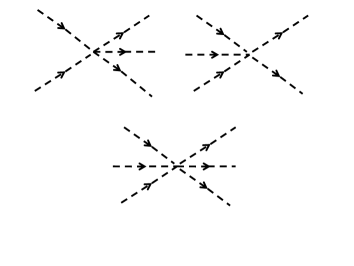
Figure 2: Feynman diagrams of the processes providing thermalization of low-energy excitations (phonons).

Figure 3: Transition matrix element ${\cal M}\equiv{\cal M}^{k_{0}-k_{1}-k_{2}\,k_{1}\,k_{2}}_{k_{0}}$ as a function of the product state wavenumber $k_{1}$. Units on axes are dimensionless. On the horizontal axis label we explicitly indicate scaling of $k_{1}$ to the inverse healing length. ${\cal M}$ is calculated on the energy shell, i.e. the energy conservation Eq. (46) holds. Solid lines: the main result of Sec. III, given by Eqs. (40 – 42). Dashed lines: approximation by Eqs. (44, 45) (singular at $k_{1}\rightarrow 0$). Initial momentum $k_{1}=10\,\zeta_{\mathrm{h}}^{-1}$ (thin lines) and $25\,\zeta_{\mathrm{h}}^{-1}$ (thick lines). Fitting by Eq. (49) is practically indistinguishable from the solid lines and is displayed in the inset.

III.2 Fast-particle limit

In this limit $k_{0}\gg 1$. As concerns the the product states, there are two distinct cases Glazman . All three product elementary excitations can be fast as well, in this case Eq.(46) yields

$$k_{2}=\frac{k_{0}-k_{1}}{2}-\frac{1}{2}\sqrt{k_{0}^{2}+2k_{0}k_{1}-3k_{1}^{2}}.$$ (50)

The aforementioned ordering convention $k_{2}<0$, $0<k_{1}<k_{0}-k_{1}-k_{2}$, $k_{0}>0$ now results in

$$0<k_{1}<2k_{0}/3.$$ (51)

But there is another possibility, when two product elementary excitations are phonons, $k_{1}\lesssim 1$ and

$$k_{2}=-\frac{k_{0}-1}{k_{0}+1}k_{1}.$$ (52)

Although the phase space corresponding to the latter case is relatively small, collisions with small transferred momentum are bosonically amplified in a quantum gas with high thermal population of phononic modes, and their contribution to the fast particle damping can be significant Glazman .

Eqs. (40 – 42) yield on the energy shell, i.e. for Eqs. (50) and (52) holding for $k_{1}\gg 1$ and $k_{1}\lesssim 1$, respectively

$${\cal M}^{k_{0}-k_{1}-k_{2}\,k_{1}\,k_{2}}_{k_{0}}=\left\{\begin{array}[]{ll}3\sqrt{|k_{1}k_{2}|}/4\,,&k_{1}\lesssim 1\\ 3/2\,,&k_{1}\gg 1\end{array}\right.\;.$$ (53)

The formula interpolating between these two cases is

$${\cal M}^{k_{0}-k_{1}-k_{2}\,k_{1}\,k_{2}}_{k_{0}}=\frac{3}{2}\sqrt{S_{k_{1}}S_{k_{2}}},$$ (54)

in full agreement with the used in Ref. Glazman assumption of correlation separation

$$\langle k_{0}-k_{1}-k_{2}\,k_{1}\,k_{2}|\hat{n}^{3}|k_{0}\rangle=3\langle k_{1}\,k_{2}|\hat{n}^{2}|0\rangle\langle k_{0}-k_{1}-k_{2}|\hat{n}|k_{0}\rangle$$ (55)

that singles out the fast particle contribution.

In Fig. 3 we display the matrix element Eq. (40) calculated in the case of $k_{0}\gg 1$ with ${\cal Y}_{q\,q^{\prime}}$, ${\cal Z}_{q\,q^{\prime}}$ given by Eqs. (41, 42), and, for comparison, its value calculated from Eqs. (43 – 45). We see that the latter approach works only for asymptotically large $k_{1}$, and the former one is in a very good agreement with the approximation (54).

Approximation (54) breaks down out of the energy shell. This can be important for transient processes, with the energy uncertainty inversely proportional to the duration of the external driving of the system, like in the experiment NirD1 . However, this problem (also related to the quantum Zeno and anti-Zeno effects KKNat ) is to be considered separately from the kinetic equation, which follows from Fermi’s golden rule and is considered in the next Section.

IV Kinetic equation

IV.1 General approach

Using Fermi’s golden rule, we can readily write a 1D kinetic equation that takes into account effects of bosonic amplification [cf. Eq. (36)]:

$$\frac{\partial}{\partial t}f_{k} = -\gamma_{0}\bigg{\{}\int\int_{Q_{12}}dk_{1}dk_{2}\,\delta(\epsilon_{k-k_{1}-k_{2}}+\epsilon_{k_{1}}+\epsilon_{k_{2}}-\epsilon_{k})\left|{\cal M}^{k-k_{1}-k_{2}\,k_{1}\,k_{2}}_{k}\right|^{2}\times$$ (56)

$$[(f_{k-k_{1}-k_{2}}+1)(f_{k_{1}}+1)(f_{k_{2}}+1)f_{k}-f_{k-k_{1}-k_{2}}f_{k_{1}}f_{k_{2}}(f_{k}+1)]+$$

$$\int\int_{Q_{12}^{\prime}}dk_{1}dk_{2}\,\delta(\epsilon_{k}+\epsilon_{k_{1}}+\epsilon_{k_{2}}-\epsilon_{k+k_{1}+k_{2}})\left|{\cal M}^{k\,k_{1}\,k_{2}}_{k+k_{1}+k_{2}}\right|^{2}\times$$

$$[f_{k}f_{k_{1}}f_{k_{2}}(f_{k+k_{1}+k_{2}}+1)-(f_{k}+1)(f_{k_{1}}+1)(f_{k_{2}}+1)f_{k+k_{1}+k_{2}}]\bigg{\}}.$$

Here $f_{k}$ is the population of the elementary excitation mode with the 1D momentum $k$. The rate of the process is scaled to $\gamma_{0}=(72/\pi)(\kappa_{\mathrm{3b}}/n_{\mathrm{1D}})^{2}$ or, in usual units,

$$\gamma_{0}=\frac{18}{\pi}\omega_{\perp}\xi^{2}\left(\frac{n_{\mathrm{1D}}a_{s}^{2}}{l_{\perp}}\right)^{2},$$ (57)

where $l_{\perp}=\sqrt{\hbar/(m\omega_{\perp})}$ is the radial trapping length scale. The first term in curly brackets in Eq. (56) corresponds to processes shown in Fig. 1 with the wave number $k$ assigned to the (single) incoming line in Fig. 1(a) or the (single) outgoing line in Fig. 1(b). The second term describes the situation of $k$ being one of the three incoming quasiparticle momenta in Fig. 1(b) or one of the three outgoing quasiparticles in Fig. 1(a). The respective integration ranges take into account the bosonic nature of elementary excitations and are defined in a way that prevents double counting of the same momenta of elementary excitations. $Q_{12}$ includes all $k_{1}$, $k_{2}$ satisfying the conditions $\mathrm{sgn}\,k_{1}=\mathrm{sgn}\,(k-k_{1}-k_{2})=-\mathrm{sgn}\,k_{2}=\mathrm{sgn}\,k$, $|k_{1}|<|k-k_{1}-k_{2}|$, $0<|k_{2}|<\infty$; $Q_{12}^{\prime}$ consists of two regions: (i) $\mathrm{sgn}\,k=\mathrm{sgn}\,k_{1}=-\mathrm{sgn}\,k_{2}=\mathrm{sgn}\,(k-k_{1}-k_{2})$, $0<|k_{1}|<\infty$, $0<|k_{2}|<\infty$, and $\mathrm{sgn}\,k=-\mathrm{sgn}\,k_{1}=-\mathrm{sgn}\,k_{2}=-\mathrm{sgn}\,(k-k_{1}-k_{2})$, $0<|k_{1}|<|k-k_{1}-k_{2}|<\infty$.

In trapped quasicondensates, Eq. (56) applies in the local density approximation if discreteness of the elementary exciation spectrum is not important, i.e., if $|k_{2}|\gg 2\pi/\ell$. Practically, this means Eq. (56) applies in the fast particle damping regime for scattering events with $|k_{1}|\approx|k_{2}|\gg 2\pi/\ell$. In this case, competing processes shown in Fig. 2 should provide relatively small contribution to the thermalization rate, however, their detailed calculation is to be a subject of future work. A rough estimation (based on evaluation of phase space available for scattering of a fast particle with wave number $k\gg 1$ on other quasiparticles) predicts that the diagrams from the first and second raws yield the rates smaller by a factor $k/n_{\mathrm{1D}}$ and $(k/n_{\mathrm{1D}})^{2}$, respectively.

It is easy to check that the stationary solution of Eq. (56) is the Bose-Einstein equilibrium distribution

$$f^{\mathrm{e}}_{k}=\frac{1}{\exp(\epsilon_{k}/T)-1}.$$ (58)

Here we measure temperature $T$ in energy units (i.e., set Boltzmann’s constant to 1). Eq. (56) does not conserve the total number of elementary excitations, therefore chemical potential in the Bose-Einstein distribution (57) is zero.

If the energy $\epsilon_{k}$ of the fast particle is much larger than both the temperature and mean interaction energy per particle then scattering with large transferred momentum populates initially empty particle-like modes, and the population of the $k$-mode decreases exponentially with the decrement $\Gamma^{\mathrm{damp}}=\sqrt{3}\pi\gamma_{0}/4$ Mazets2 ; Glazman (note that $\Gamma^{\mathrm{damp}}$ does not depend on $k$).

It has been noticed Glazman that three-body collisions with small momentum transfer can give, due to bosonic amplification, major contribution to the damping rate of a fast particle in a certain parameter range. In the present paper we make a step forward compared to the treatment of Ref. Glazman by looking precisely to the dynamics of a bunch of fast particles in a 1D quasicondensate.

IV.2 Fokker-Planck equation

We consider a non-equilibrium distribution of elementary excitations $f_{k}=f_{k}^{\mathrm{e}}+\delta f_{k}$, where the perturbed part is small, $\int_{-\infty}^{\infty}dk\,\delta f_{k}\ll\int_{-\infty}^{\infty}dk\,f_{k}^{\mathrm{e}}$, and is localized in the momentum space around $k_{0}\gg 1$ (the width of the fast particles bunch being $\Delta k\ll k_{0}$). Such a distribution can be created by means of Bragg spectroscopy Bragg1 , perhaps, using higher-order processes Bragg2 to obtain large values of $k_{0}$. To be still in the 1D regime and avoid scattering of atoms to radially excited states we must require the kinetic equation of the fast particles to be lees than $2\hbar\omega_{\perp}$ (factor 2 appears here due to parity conservation Mazets1 ; Mazets2 ). A relatively small numbers of fast particles allows us to neglect heating of the lower modes in the course evolution.

In what follows we take into account only collisions with small momentum transfer. Then we analyze the dynamics of $\delta f_{k}$ on the time scale much shorter than $1/\Gamma^{\mathrm{damp}}$ (when we can neglect scattering with large momentum transfer). A change of $\delta f_{k}$ on such a short time scal will be a measure of the importance of the scattering events with the small momentum transfer, bosonically-amplified by $f_{k_{1}}^{\mathrm{e}}\sim f_{k_{2}}^{\mathrm{e}}\gg 1$.

The assumptions listed above enable us to linearize the kinetic equation (56) and reduce it to the Fokker-Planck equation Gardiner . We neglect the momentum dependence of the kinetic coefficients (diffusion $D$ and advection $A$ within the narrow momentum around $k_{0}$ and finally obtain

$$\frac{\partial}{\partial t}\delta f_{k}=A\frac{\partial}{\partial k}\delta f_{k}+D\frac{\partial^{2}}{\partial k^{2}}\delta f_{k},$$ (59)

$$A = \gamma_{0}\int_{0}^{\infty}dk_{1}\int_{-\infty}^{0}dk_{2}\,(k_{1}+k_{2})\left|{\cal M}^{k_{0}-k_{1}-k_{2}\,k_{1}\,k_{2}}_{k_{0}}\right|^{2}\delta(\epsilon_{k_{0}-k_{1}-k_{2}}+\epsilon_{k_{1}}+\epsilon_{k_{2}}-\epsilon_{k_{0}})(f_{k_{1}}^{\mathrm{e}}+f_{k_{2}}^{\mathrm{e}}),$$ (60)

$$D = \gamma_{0}\int_{0}^{\infty}dk_{1}\int_{-\infty}^{0}dk_{2}\,(k_{1}+k_{2})^{2}\left|{\cal M}^{k_{0}-k_{1}-k_{2}\,k_{1}\,k_{2}}_{k_{0}}\right|^{2}\delta(\epsilon_{k_{0}-k_{1}-k_{2}}+\epsilon_{k_{1}}+\epsilon_{k_{2}}-\epsilon_{k_{0}})[f_{k_{1}}^{\mathrm{e}}f_{k_{2}}^{\mathrm{e}}+(f_{k_{1}}^{\mathrm{e}}+f_{k_{2}}^{\mathrm{e}})/2].~{}$$ (61)

Eqs. (59 – 61) are written still in dimensionless variables. In what follows we assume usual time and length units in Eqs. (59) and evaluate $A$ and $D$ in two limiting cases. First, for $T\lesssim g_{\mathrm{1D}}n_{\mathrm{1D}}$ we obtain

$$A \approx 14.6\,\mathrm{sgn}\,k_{0}\,\frac{\gamma_{0}}{|k_{0}|^{2}\zeta_{h}^{3}}\left(\frac{T}{g_{\mathrm{1D}}n_{\mathrm{1D}}}\right)^{4},$$ (62)

$$D \approx 2.45\,\frac{\gamma_{0}}{|k_{0}|^{3}\zeta_{h}^{5}}\left(\frac{T}{g_{\mathrm{1D}}n_{\mathrm{1D}}}\right)^{5},$$ (63)

where $\gamma_{0}$ is given by Eq. (57).

If, on the contrary, $g_{\mathrm{1D}}n_{\mathrm{1D}}\ll T\lesssim 2\hbar\omega_{\perp}$ then bosonic amplification of scattering to free-particle-like mode becomes significant and we obtain

$$A \approx 14.7\,\mathrm{sgn}\,k_{0}\,\frac{\gamma_{0}}{|k_{0}|^{2}\zeta_{h}^{3}}\left(\frac{T}{g_{\mathrm{1D}}n_{\mathrm{1D}}}\right)^{3/2},$$ (64)

$$D \approx 10.8\,\frac{\gamma_{0}}{|k_{0}|^{3}\zeta_{h}^{5}}\left(\frac{T}{g_{\mathrm{1D}}n_{\mathrm{1D}}}\right)^{5/2}.$$ (65)

The decrease of the kinetic coefficients $A$ and $D$ with growing $k_{0}$ is explained by two observation. First, the total momentum transfer decreases as $k_{0}$ increases but the low-energy excitation momentum $k_{1}$ is kept fixed (and $k_{2}$ is related to $k_{0}$ and $k_{1}$ via energy and momentum conservation): $k_{1}+k_{2}\approx|k_{1}|(4\zeta_{\mathrm{h}}^{-2}+k_{1}^{2})^{1/2}/k_{0}$. Second, integrating in Eqs. (60, 61) the delta-function of the energy difference over $k_{2}$ yields another factor $1/k_{0}$.

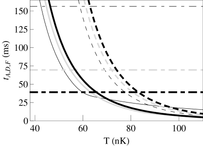
Figure 4: Typical times of shift ($t_{A}$, solid lines), diffusion ($t_{D}$, dashed lines), and scattering with large momentum transfer ($t_{F}\equiv 1/\Gamma^{\mathrm{damp}}$, dot-dashed lines) for ⁸⁷Rb quasicondensate with $n_{\mathrm{1D}}=40\;\mu\mathrm{m}^{-1}$ (thin black lines), $60\;\mu\mathrm{m}^{-1}$ (medium gray lines), and $80\;\mu\mathrm{m}^{-1}$ (thick black lines) as functions of temperature. $\omega_{\perp}=2\pi\times 3$ kHz. Initial distribution of fast atoms is Gaussian with the mean $k_{0}=\sqrt{2m\omega_{\perp}/\hbar}=0.7\times 10^{5}\;\mathrm{cm}^{-1}$ and the r.m.s. $\Delta k=\frac{1}{4}k_{0}$.

Assume that the initial distribution of fast particles is Gaussian, centered at $k_{0}$ and with r.m.s (determined, for example, by the duration of the Bragg pulse Bragg1 ) $\Delta k$. The well-known solution Gardiner of Eq. (59) with the Gaussian initial condition is $\delta f_{k}(t)\propto\exp[-(k-k_{0}+At)^{2}/(2\Delta k^{2}+4Dt)]/(2\Delta k^{2}+4Dt)^{1/2}$. We define the typical time scales $t_{A}$ and $t_{D}$ as times when shift of the maximum of $\delta f_{k}$ or increase of its width, respectively, become comparable to the initial width $\Delta k$:

$$t_{A}=\Delta k/A,\qquad t_{D}=\Delta k^{2}/(2D).$$ (66)

Bosonically-amplified three-body collisions with small momentum transfer are practically important, if they modify $\delta f_{k}$ faster, than scattering with large momentum transfer to initially empty modes, i.e., if at least one of two inequalities

$$\Gamma^{\mathrm{damp}}t_{A}\lesssim 1,\qquad\Gamma^{\mathrm{damp}}t_{D}\lesssim 1$$ (67)

is satisfied. Note, that the number of scattering events per unit time per one fast atom can be significantly larger than $\Gamma^{\mathrm{damp}}\approx 1.36\,\gamma_{0}$, but their influence on the dynamics of the distribution $\delta f_{k}$ may be still small.

Fig. 4 illustrates $t_{A}$, $t_{D}$ juxtaposed with $t_{F}\equiv 1/\gamma^{\mathrm{damp}}$ for experimentally realistic system parameters. One can see that, at experimentally feasible densities, first the momentum-shift time $t_{A}$ and then the diffusion time $t_{D}$ become shorter than the typical time $t_{F}$, as temperature increases. However, we should always keep in mind the limitation $T\lesssim\hbar\omega_{\perp}$ necessary for the 1D regime.

Now we can compare our criterion for the significance of the small-transferred-momentum scattering events and that proposed by Tan, Pustilnik and Glazman Glazman . In the latter case, the small-transferred-momentum scattering events were considered important if the total collision rate per atom far exceeded the value of $\Gamma^{\mathrm{damp}}$. This corresponds, in the limit

$$k_{0}\zeta_{\mathrm{h}}\gg 1,$$ (68)

to temperatures $T\gtrsim g_{\mathrm{1D}}n_{\mathrm{1D}}(k_{0}\zeta_{h})^{1/2}$. We show, that this condition is not sufficient for experimental observation of the effect of these collisions, and require Eq. (67) instead. The shift of the mean momentum of fast particles becomes significant at

$$T\gtrsim g_{\mathrm{1D}}n_{\mathrm{1D}}(k_{0}\zeta_{h})^{4/3}(\Delta k\zeta_{h})^{2/3}=\frac{\hbar^{2}k_{0}^{4/3}\Delta k^{2/3}}{m},$$ (69)

and large diffusive spreading of the momentum distribution of fast particles requires

$$T\gtrsim g_{\mathrm{1D}}n_{\mathrm{1D}}(k_{0}\zeta_{h})^{6/5}(\Delta k\zeta_{h})^{4/5}=\frac{\hbar^{2}k_{0}^{6/5}\Delta k^{4/5}}{m}.$$ (70)

Note that Eq. (68) does not hold for standard two-photon Bragg spectroscopy Bragg1 , which can provide $k_{0}\zeta_{\mathrm{h}}\sim 5$. In this case, a rough estimation yields, instead of Eq.(69, 70), $T\gtrsim g_{\mathrm{1D}}n_{\mathrm{1D}}$ (cf. Fig. 4).

V Discussion and conclusions

Eq. (67) is not the only restriction that applies in a real experiment. In practice, we always need to take into account the finiteness of the system. The longitudinal trapping determines the finite size of the ultracold atomic cloud radius . This size can be associated, by order of magnitude, with the parameter $\ell$ introduced in Sec. III.1. The longitudinal trapping potential itself lifts, in principle, the integrability of the Lieb-Liniger model, however, we expect this non-integrability effect to be small ti11 . More important is anharmonicity (of the longitudinal trap itself or induced by the atomic mean-field interactions) that induces dephasing and thus limits the time of observation of the integrable dynamics to few oscillation periods WeissNC . The most desirable case takes place if the bosonically-amplified three-body elastic processes manifest themselves after a single passage of fast atoms through the cloud, i.e. on the time scale $\tau_{0}=m\ell/(\hbar k_{0})$. The Bragg pulse that produces the fast atoms should be also much shorter than $\tau_{0}$. In contrast to the Fourier-limited width of the excitation spectrum in the frequency domain, the momentum distribution width $\Delta k\approx mT/(2\hbar^{2}{n}_{\mathrm{1D}})$ of the fast particles is determined by thermal fluctuations of the phase of the quasicondensate Aspect1 . Regarding a longitudinally trapped quasicondensate, we will use the notation ${n}_{\mathrm{1D}}$ for its average linear density. Although the momentum distribution is Lorentzian Aspect1 ; Aspect2 , we still use Eq. (66), which is derived in the case of a Gaussian, for rough estimations. We assume that, after the Bragg pulse, fast atoms are left to interact with the rest of the quasicondensate for the time $t_{\mathrm{int}}\sim\tau_{0}$. Then the trap is suddenly switched off, and the atomic cloud expands ballistically. The atomic position distribution in the asymptotic regime of long time of flight corresponds to the in-trap momentum distribution Bragg1 . We assume that the influence of the bosonically amplified three-body collisions with small momentum transfer is unambiguously detectable if the relative shift of the momentum of fast stoms due to three-body elastic scattering is of about 50%, i.e. $At_{\mathrm{int}}\approx 0.5\,k_{0}$. To be definite, consider an atomic cloud of size $\ell\approx 100~{}\mu$m. Initial wave number $k_{0}=0.7\times 10^{5}\;\mathrm{cm}^{-1}$ of the fast particles corresponds to $\tau_{0}\approx 20$ ms. Taking $t_{\mathrm{int}}=10$ ms, we find that the bosonically-amplified three-body scattering is detectable at $T>110$ nK for $n_{\mathrm{1D}}=80~{}\mu\mathrm{m}^{-1}$ and $T>140$ nK for $n_{\mathrm{1D}}=60~{}\mu\mathrm{m}^{-1}$. The linear density $n_{\mathrm{1D}}=40~{}\mu\mathrm{m}^{-1}$ is too small, and the slowing down of fast particles can not be seen in the temperature range corresponding to the 1D regime. Note for all these density values $\Gamma^{\mathrm{damp}}t_{\mathrm{int}}<1$, i.e. three-body scattering into empty modes (with lage momentum transfer) is too weak to be detected in a singe passage of fast atoms through the quasicondensate.

An alternative (to Bragg spectroscopy) way of producing fast atoms in twin-atom beams by external driving of the radial excitations of ultracold atoms in an elongated trap has been recently demonstrated by Bücker et al. Bue .

Finally, we discuss the relation between the theory of ultracold atomic systems in the quasi-1D regime and the quantum Newton’s cradle experiment WeissNC that has brought a new attention to the problem of the integrability breakdown. Thermalization has not been observed in that experiment, and only lower limits to the thermalization time have been obtained for different (strong and intermediate) interaction strengths WeissNC . This fact is in a quantitative agreement with the estimations of the thermalization rate Glazman (see also Ref. Mazets2 ) taking into account the effect of the atomic correlations [the zero-distance two-body correlation function $g_{2}(0)<1$] in the case of strong repulsive interactions. The damping time $1/[\gamma_{0}g_{2}(0)]$ occurs to be too long to be measured. Also a small size of the colliding atomic clouds puts a relatively high infrared momentum cut-off ($2\pi/\ell>0.1~{}\mu\mathrm{m}^{-1}$) that precludes scattering events with small momentum transfer. As we mentioned before, non-integrability caused by the longitudinal harmonic confinement is also too weak to be detected ti11 . Another possible mechanism of the non-integrability, associated with the tunnel coupling between adjacent waveguides in a 2D optical lattice, can be relevant only for optical lattices much weaker than that applied in Ref. WeissNC . To observe thermalization of bosonic atoms in a quasi-1D waveguide and, in particular, to test the theory developed in the present paper, one has to work at larger atom numbers that provide both higher atomic linear densities and longer system sizes than in the quantum Newton’s cradle experiment WeissNC .

To summarize, in this paper we analyzed effective three-body collisions (mediated by virtual excitations of the radial degrees of freedom) in a 1D quasicondensate of ultracold bosonic atoms. We calculated the matrix element for the decay of a single elementary excitations into three elementary excitations. We stress that the obtained expression is non-divergent at small momentum transfer. We derived a kinetic equation governing the damping of fast particles in a quasicondensate and its Fokker-Planck limit that accounts for scattering into thermally populated modes with small momenta. We demonstrate that the latter process can be observed experimentally.

The author thanks J. Armijo, I. Bouchoule, L. I. Glazman, H. Grosse, S. Manz, J. Schmiedmayer, and J. Yngvason for helpful discussions. This work is supported by the FWF (project P22590-N16).

References

- (1) E. H. Lieb and W. Liniger, Phys. Rev. 130, 1605 (1963); E. H. Lieb, Phys. Rev. 130, 1616 (1963).
- (2) H. B. Thacker, Rev. Mod. Phys. 53, 253 (1981).
- (3) T. Kinoshita, T. R. Wenger and D. S. Weiss, Science 305, 1125 (2004); O. Morsch and M. Oberthaler, Rev. Mod. Phys. 78, 179 (2006).
- (4) R. Folman, P. Krüger, D. Cassettari, B. Hessmo, T. Maier, and J. Schmiedmayer, Phys. Rev. Lett. 84, 4749 (2000); J. Fortágh and C. Zimmermann, Rev. Mod. Phys. 79, 235 (2007).
- (5) M. Olshanii, Phys. Rev. Lett. 81, 938 (1998).
- (6) Note that it is practically sufficient to have temperature and the mean-field interaction energy slightly below (or even comparable to) to ensure the 1D regime, as demonstrated in many experiments: S. Manz, R. Bücker, T. Betz, Ch. Koller, S. Hofferberth, I. E. Mazets, A. Imambekov, E. Demler, A. Perrin, J. Schmiedmayer, and T. Schumm, Phys. Rev. A 81, 031610 (2010); P. Krüger, S. Hofferberth, I. E. Mazets, I. Lesanovsky, and J. Schmiedmayer, Phys. Rev. Lett. 105, 265302 (2010); T. Betz, S. Manz, R. Bücker, T. Berrada, Ch. Koller, G. Kazakov, I. E. Mazets, H.-P. Stimming, A. Perrin, T. Schumm, and J. Schmiedmayer, Phys. Rev. Lett. 106, 020407 (2011).
- (7) T. Kinoshita, T. Wenger, and D. S. Weiss, Nature 440, 900 (2006).
- (8) S. Hofferberth, I. Lesanovsky, T. Schumm, A. Imambekov, V. Gritsev, E. Demler, and J. Schmiedmayer, Nature Physics 4, 489 (2008).
- (9) L. Salasnich, A. Parola, and L. Reatto, Phys. Rev. A 65, 043614 (2002).
- (10) A. Muryshev, G. V. Shlyapnikov, W. Ertmer, K. Sengstock, and M. Lewenstein, Phys. Rev. Lett. 89, 110401 (2002).
- (11) L. Khaykovich and B. A. Malomed, Phys. Rev. A 74, 023607 (2006); L. Salasnich and B. A. Malomed, Phys. Rev. A 74, 053610 (2006).
- (12) I. E. Mazets, T. Schumm, and J. Schmiedmayer, Phys. Rev. Lett. 100, 210403 (2008).
- (13) I. E. Mazets and J. Schmiedmayer, New J. Phys. 12, 055023 (2010).
- (14) S. Tan, M. Pustilnik, and L. I. Glazman, Phys. Rev. Lett. 105, 090404 (2010).
- (15) V. N. Popov, Functional Integrals in Quantum Field Theory and Statistical Physics (Reidel, Dordrecht, 1983).
- (16) C. Mora and Y. Castin, Phys. Rev. A 67, 053615 (2003).
- (17) M. Lewenstein and L. You, Phys. Rev. Lett. 77, 3489 (1996).
- (18) S. T. Beliaev, Sov. Phys. JETP 34, 299 (1958).
- (19) W. V. Liu, Phys. Rev. Lett. 79, 4056 (1997).
- (20) P. C. Hohenberg and P. C. Martin, Ann. Phys. (N. Y.) 34, 291 (1965).
- (21) A. Ishihara, Statistical Physics (Academic Press, New York, 1971).
- (22) J. J. Sakurai, Modern Quantum Mechanics (Addison-Wesley, Reading MA, 1994).
- (23) M.-C. Chung and A. B. Bhattacherjee, New J. Phys. 11, 123012 (2009).
- (24) N. Bar-Gill, E. E. Rowen, G. Kurizki, and N. Davidson, Phys. Rev. Lett. 102, 110401 (2009).
- (25) A. G. Kofman and G. Kurizki, Nature 405, 546 (2000).
- (26) D. M. Stamper-Kurn, A. P. Chikkatur, A. Görlitz, S. Inouye, S. Gupta, D. E. Pritchard, and W. Ketterle, Phys. Rev. Lett. 83, 2876 (1999); J. Steinhauer, R. Ozeri, N. Katz, and N. Davidson, Phys. Rev. Lett. 88, 120407 (2002).
- (27) E. E. Rowen, N. Bar-Gill, and N. Davidson, Phys. Rev. Lett. 101, 010404 (2008)
- (28) C. W. Gardiner, Stochastic Methods (Springer, Berlin, 2009).
- (29) J. N. Fuchs, X. Leyronas, and R. Combescot, Phys. Rev. A 68, 043610 (2003); F. Gerbier, Europhys. Lett. 66, 771 (2004).
- (30) I. E. Mazets, arXiv: 1011.0713 (accepted for publication in Eur. Phys. J. D).
- (31) S. Richard, F. Gerbier, J. H. Thywissen, M. Hugbart, P. Bouyer, and A. Aspect, Phys. Rev. Lett. 91, 010405 (2003).
- (32) The shape and the width of the momentum distribution of atoms decoupled by the Bragg pulse Aspect1 are in a good agreement with their estimation from the Fourier transform of the first-order spatial correlation function of a weakly-interacting quasicondensate Popov ; MC .
- (33) R. Bücker, J. Grond, S. Manz, T. Berrada, T. Betz, Ch. Koller, U. Hohenester, T. Schumm, A. Perrin, and J. Schmiedmayer, arXiv: 1012.2348.