Large-deviation principles, stochastic effective actions, path entropies, and the structure and meaning of thermodynamic descriptions

Abstract

The meaning of thermodynamic descriptions is found in large-deviations scaling Ellis:ELDSM:85 ; Touchette:large_dev:08 of the probabilities for fluctuations of averaged quantities. The central function expressing large-deviations scaling is the entropy, which is the basis for both fluctuation theorems and for characterizing the thermodynamic interactions of systems. Freidlin-Wentzell theory Freidlin:RPDS:98 provides a quite general formulation of large-deviations scaling for non-equilibrium stochastic processes, through a remarkable representation in terms of a Hamiltonian dynamical system. A number of related methods now exist to construct the Freidlin-Wentzell Hamiltonian for many kinds of stochastic processes; one method due to Doi Doi:SecQuant:76 ; Doi:RDQFT:76 and Peliti Peliti:PIBD:85 ; Peliti:AAZero:86 , appropriate to integer counting statistics, is widely used in reaction-diffusion theory.

Using these tools together with a path-entropy method due to Jaynes Jaynes:caliber:80 , this review shows how to construct entropy functions that both express large-deviations scaling of fluctuations, and describe system-environment interactions, for discrete stochastic processes either at or away from equilibrium. A collection of variational methods familiar within quantum field theory, but less commonly applied to the Doi-Peliti construction, is used to define a “stochastic effective action”, which is the large-deviations rate function for arbitrary non-equilibrium paths.

We show how common principles of entropy maximization, applied to different ensembles of states or of histories, lead to different entropy functions and different sets of thermodynamic state variables. Yet the relations of among all these levels of description may be constructed explicitly and understood in terms of information conditions. Although the example systems considered are limited, they are meant to provide a self-contained introduction to methods that may be used to systematically construct descriptions with all the features familiar from equilibrium thermodynamics, for a much wider range of systems describable by stochastic processes.

I Introduction

Thermodynamics is not fundamentally a theory of energy distribution, but a theory of statistical degeneracy Jaynes:LOS:03 . As such, while most of our experience and intuition about thermodynamics is drawn from equilibrium statistical mechanics Fermi:TD:56 ; Kittel:TP:80 ; Huang:SM:1987 , which emphasizes the role of energy, we should expect that its fundamental principles apply in much wider domains, outside equilibrium, and even outside mechanics.

Within the last 50 years, a clear conceptual understanding of the nature of thermodynamic descriptions Ellis:ELDSM:85 ; Touchette:large_dev:08 has combined with new methods to analyze a wide variety of stochastic processes, for continuous Martin:MSR:73 and discrete systems Doi:SecQuant:76 ; Doi:RDQFT:76 ; Peliti:PIBD:85 ; Peliti:AAZero:86 , in quantum Schwinger:MBQO:61 ; Keldysh::65 and classical mechanics Mattis:RDQFT:98 ; Cardy:FTNEqSM:99 , both at and away from equilibrium, and even in other areas using information theory such as optimal data compression and reliable communication Shannon:MTC:49 , and via these, robust molecular recognition Schneider:TMMI:91 ; Schneider:TMMII:91 . These developments confirm that thermodynamics is indeed not restricted to equilibrium or to mechanics. They give us insight into when thermodynamic descriptions should exist, and they provide systematic methods to construct such descriptions in a wide variety of situations.

This paper reviews the aspects of large-numbers scaling and structural decomposition that are essential to thermodynamic descriptions, and presents examples from which each of these may be seen in different forms that are appropriate to equilibrium and non-equilibrium statistical mechanics. It also brings together construction methods (based on generating functions Doi:SecQuant:76 ; Doi:RDQFT:76 ; Peliti:PIBD:85 ; Peliti:AAZero:86 ), scaling relations (based on ray approximations Graham:path_int:77 ; Freidlin:RPDS:98 ), and variational methods (based on functional Legendre transforms Weinberg:QTF_II:96 ), which will enable the reader to systematically construct the fluctuation theorems of thermodynamic descriptions from their underlying stochastic processes.

I.1 Key concepts, and source of examples

I.1.1 Entropy underlies large-deviations scaling and reflects system structure

The entropy, as a logarithmic measure of degeneracy, is the central quantity in thermodynamics. It arises as the leading term in the log-probability for fluctuations of averaged quantities. At the same time, however, when sub-system components, or a system and its environment, interact, they discover their most probable joint configuration through fluctuations. Therefore the competition among entropy terms also reflects the structure of system interactions at the macroscale. We are reminded of the importance of this structural role of entropies, by the fact that pure “classical” thermodynamics Fermi:TD:56 is entirely devoted to the analysis of entropy gradients. Therefore we wish to insist on being able to decompose entropy into its sub-system components as a criterion for any fully-developed thermodynamic description.

The key property that defines the existence of thermodynamic limits, and the form of their fluctuation theorems, is large-deviations scaling Ellis:ELDSM:85 ; Touchette:large_dev:08 . It is the precise statement of the simplification provided by the law of large numbers, not only in the infinite limit of aggregation, but in the asymptotic approach to infinity. It is well-known that averaging over ensembles of configurations for large systems removes almost all (irrelevant) degrees of freedom, and leaves only summary statistics, which are the state variables of the thermodynamic description. In finite systems, these summary statistics can still show sample fluctuation, but in the thermodynamic limit, the fluctuation probability takes a simple form.

For an ensemble that possesses large-deviations scaling, it is possible to describe classes of fluctuations as having the same structure under different degrees of aggregation. (An example would be fractional density fluctuations in regions of a gas, whose sample volume may be varied). The log-probability for any such fluctuation then factors, into a term that depends on overall system scale, and a scale-invariant coefficient that depends only on the structure of the fluctuation. The scale-invariant coefficient is called the rate function of the large-deviations scaling relation Touchette:large_dev:08 . (An example would be the specific entropy of a gas.)

Large-deviations scaling presumes the existence of a separation of scales – between microscopic processes and their macroscopic descriptions – over which aggregation does not lead to qualitative changes in the kinds of fluctuations that can occur. We expect thermodynamic limits to exist where this separation of scales is large. Examples of structural change that can interrupt simple scaling under the law of large numbers include phase transitions, which can change the space of accessible excitations.

Large-deviations scaling permits us to combine fluctuation statistics with entropy decompositions that reflect system structure. In equilibrium thermodynamics, the result is the classical fluctuation theorem for macrostates Ellis:ELDSM:85 : the log-probability for fluctuations (of energy, volume, particles, etc.) between sub-systems with well-defined entropies is the difference between the sum of entropies at the fluctuating value and the maximum value for this sum, which is the equilibrium value.

If we wish to consider the probabilities of fluctuations with more complex structure (whether in equilibrium thermodynamics or in more complicated cases), we will need more flexible methods to compute large-deviations formulae and entropy decompositions. For this, we introduce the notion of the stochastic effective action, which is defined by variational methods that generalize the familiar Legendre transform of equilibrium thermodynamics. The meaning of this quantity, and the way it is used, will be most easily understood by following its construction in the body of the paper, so we postpone further discussion until that point.

I.1.2 The principles in a simple progression: from equilibrium to non-equilibrium statistical mechanics

We will develop examples whose purpose is to show that the definition and properties of the entropy do not change as we extend thermodynamics beyond equilibrium statistical mechanics. Rather, what changes is the state space to which we assign probabilities.

A direct example comes from comparing an equilibrium thermodynamic system, to a non-equilibrium description constructed for the same system. A frequent approach Onsager:RRIP1:31 ; Onsager:RRIP2:31 ; DeGroot:NET:84 ; Prigogine:MT:98 to non-equilibrium statistical mechanics (NESM) continues to use the equilibrium state variables and equilibrium entropy, but considers their time rates of change. We will see that such an approach, focused on retaining the functional form of the equilibrium entropy, sacrifices its meaning as a large-deviations rate function.

Instead, we will make the transition from equilibrium to non-equilibrium statistical mechanics by replacing an ensemble of states (in equilibrium) by an ensemble in which entire time-dependent trajectories – termed histories – are the elementary entities (for NESM), and then we will construct the appropriate large-deviations limits for the ensemble of histories. The functional form of the entropy will necessarily change. More importantly, the inventory of state variables will necessarily be enlarged, to include not only the configuration variables of equilibrium, but also a collection of currents that relate to the changes in configuration. Both kinds of variables will be needed as summary statistics for an ensemble of histories, and both will enter as arguments in the non-equilibrium entropy.

NESM is not so far removed from equilibrium thermodynamics that it can really do justice to the generality of large-deviations principles and thermodynamic descriptions. However, it allows us to begin with a completely familiar (equilibrium) construction, then to compare it to a construction with rather different functional forms, and finally to derive the complete set of relations that connect the two descriptions.

I.2 Markovian stochastic processes, the two-state model as an example, and the approach of the paper

Markovian stochastic processes Durrett:Stoch_Proc:99 provide a general, substrate-independent framework within which to study statistical degeneracy and large-deviations scaling. They include models from statistical mechanics, but they may also be used to represent many other random processes, whose structure may have different constraints and interpretations from those of mechanics.

This review will use the two-state random walk, in either discrete or continuous time, as a sample system for which equilibrium and non-equilibrium thermodynamic descriptions will be built and then compared. The two-state random walk is the simplest discrete stochastic process, and most thermodynamic quantities of interest in both ensembles can be computed for this system in closed form. However, the constructions in the examples immediately generalize to more complicated cases, and several generalizations and approximation methods will be covered either in the main text or in appendices.

Sec. II will introduce large-deviations scaling one level “below” the discrete random walk, by supposing that the discrete model emerges as a coarse-grained description from the continuous random walk in a double-well potential. The continuum model illustrates the concept of concentration of measure from large-deviations theory, and sets the parameters (both explicit and implicit) that define the discrete model. It also clarifies the nature and origin of the “local-equilibrium” approximation Prigogine:MT:98 for coarse-grained descriptions of motion on free-energy landscapes, and illustrates graphically the dual roles that charges and currents must have in non-equilibrium entropy principles.

Sections III and IV present the equilibrium thermodynamics of the two-state model, and its most direct generalization through the master equation of the stochastic process. Sec. III uses the exact solution of the equilibrium distribution to introduce all basic quantities of the large-deviations theory, and derives these using generating functions and their associated variational methods. Sec. IV then presents the same construction for the time-dependent probability distribution, in which histories of particle counts rather than counts at a single time are the elementary entities. Neither of these ensembles distinguishes particle identities, either in states or in trajectories. Sec. V presents an alternative construction of a thermodynamics of histories based on the entropy of distinguishable-particle trajectories, and this second construction naturally separates the path entropy from probability terms due to the environment, in a form exactly analogous to the Gibbs free energy for equilibrium.

The remainder of the introduction lists sources for the particular methods used in later sections, and explains why they capture different aspects of a full non-equilibrium thermodynamics. Many aspects of the following derivations – the naturalness of the generating-function representation, the role of operator algebras and linear algebra more generally, or the information conditions and counting statistics that relate one ensemble to another – may be understood in conceptual terms that are more fundamental than the particular constructions in which they appear below. We return to these in the discussion, making use of examples from the text.

Numerous, diverse literatures now contribute to the understanding of methods closely related to those used below. A brief summary of the history and connections among the ideas, and a broader set of citations, are provided in App. A.

I.3 Bringing together three perspectives on non-equilibrium thermodynamics

The extension of large-deviations scaling to ensembles of histories is given by Freidlin-Wentzell (F-W) theory Freidlin:RPDS:98 . This approach is widely applied to the computation of escape trajectories and first-passage times Maier:escape:93 ; Maier:non_grad:92 ; Maier:exit_dist:97 ; Maier:caustics:93 ; Maier:scaling:96 ; Maier:bifurc:00 ; Maier:oscill:96 ; Maier:sloshing:01 ; Maier:droplets:01 . It is remarkable for the way it reduces both problems of inference, and the description of multiscale dynamics, to a representation which is a Hamiltonian dynamical system Eyink:action:96 ; Mattis:RDQFT:98 .

A convenient method for arriving at the Hamiltonian description of F-W theory is the Doi-Peliti (D-P) construction Doi:SecQuant:76 ; Doi:RDQFT:76 ; Peliti:PIBD:85 ; Peliti:AAZero:86 based on generating functionals. The D-P construction is only one of many closely-related methods based on expansions in coherent states, which are reviewed in App. A. These methods Martin:MSR:73 ; Graham:path_int:77 ; Graham:potential:84 ; Kamenev:DP:01 have the common feature that the field representing sample-mean values of observables is augmented by a conjugate momentum that generates the change in those observables. This value/momentum pair leads to the F-W Hamiltonian description. The D-P method is particular to stochastic processes with independent, discrete number counts, but may readily be generalized to continuous or non-independent observables Smith:DP:08 , as well as having many parallels in dissipative quantum mechanics Schwinger:MBQO:61 ; Keldysh::65 ; Lifshitz:LandL:80 .

The F-W method directly gives the scale factors and rate functions of the large-deviations limit for histories. However, it does not generally decompose fluctuation probabilities into separate terms representing sub-system components or system-environment interactions, which we want as part of a thermodynamic description. To produce that decomposition, we introduce a path-entropy method due to Jaynes known as maximum caliber Jaynes:caliber:80 , which has its roots in much older analysis of the entropy rates of stochastic processes and chaotic dynamical systems due to Kolmogorov and others. In addition to making the F-W representation more recognizable as a direct counterpart to the constructions in equilibrium thermodynamics, the maximum-caliber method will separate those events that involve energy exchange with the environment from those that do not, allowing us to understand the role of energy dissipation in large-deviations formulae for paths.

I.4 A glossary of notation

In characterizing thermodynamic ensembles, we will need to make three choices about the level of representation, and the basis used:

1. Whether we are referring to ensemble averages (hence, deterministic summary statistics), or quantities that fluctuate stochastically to represent the process of sampling;

2. Whether we are considering discrete samples that change in the integer basis of particle counts, or modes of collective fluctuation, which we describe with the continuous mean values of Poisson distributions;

3. Whether we are describing absolute particle numbers distributed among states, or are separating total number as a scaling variable, from the fractional distributions of particles that have a scale-invariant meaning.

Different choices will lead to objects with quite different mathematical behavior, even if all of them represent particle numbers in one way or another. The notation in the following sections is chosen to reflect the three choices above, while still permitting readable equations.

Ensemble averages of any quantities are denoted by overbars. This convention is easier to incorporate in complicated equations than the $E$ (for expectation value) commonly used in statistics.

The remaining distinctions in the notation are summarized in Table 1.

Position	Domain	Measure	Dynamics	Meaning and usage	Conjugate
variable					momentum
$N$	$\left[0,\infty\right]$	Integer	Fixed	Total population number	not used
				Scale factor in large-deviations property
${\rm n}_{i}$	$\left[0,N\right]$	Integer	Stochastic	Values of sample points	$-\partial/\partial{\rm n}_{i}$
$n_{i}$	$\left[0,N\right]$	Real	Langevin	Mean of Poisson distribution	${\eta}_{i}$
${\hat{\rm n}}_{i}\equiv{\rm n}_{i}/N$	$\left[0,1\right]$	Rational	Stochastic	Relative values of sample points	$-\left(1/N\right)\partial/\partial{\hat{\rm n}}_{i}$
${\nu}_{i}\equiv n_{i}/N$	$\left[0,1\right]$	Real	Langevin	Distribution normalized by $N$	${\eta}_{i}$
				Structure factor in large-deviations property

Table 1: Notations for particle number in different bases. ${\rm n}_{i}$ are integer sample values of particle counts in state $i$. $n_{i}$ are the corresponding continuous mean values of Poisson distributions used as a basis for collective fluctuations. ${\hat{\rm n}}_{i}$ are integer sample values normalized by total number $N$ to isolate large-deviations scaling, and ${\nu}_{i}$ are the corresponding normalized mean values of Poisson distributions. Each representation of population numbers is accompanied by a conjugate momentum or shift operator, shown in the last column. Total population $N$ will be kept fixed in all examples, and its corresponding shift operator is therefore not used.

It will be important, in following the Doi-Peliti construction below, to understand that math-italic $n_{i}$ are the mean values of Poisson distributions that are used as a basis in which to expand the actual distribution that evolves under the stochastic process. They remain random variables that are sampled from the ensemble, but they fluctuate with Langevin statistics rather than the Poisson statistics of the integer particle counts ${\rm n}_{i}$. The ensemble mean will be denoted ${\bar{n}}_{i}$.

The dynamics of a stochastic process may be represented in three ways associated with these different bases, which contain equivalent information and which will all be illustrated in the following sections. These are: 1) the transfer matrix of the discrete stochastic process, which shifts probability among indices; 2) the Liouville operator that acts on generating functions, shifting probability among modes; and 3) the action functional of the Doi-Peliti field-theoretic expansion in Poisson distributions, which generates the covariance for Langevin statistics. We will show that, with a suitable choice of dynamical variables, one may skip over the laborious task of interconverting these representations, and simply copy the functional forms from one representation to another. The number variables and shift operators in Table 1 are those that substitute for one another under changes of representation.

II Large-deviations scaling and the separation of scales: concentration of measure; the skeletons for equilibrium versus dynamics; nature of the local-equilibrium approximation; existence of a natural scale

In later sections, the two-state random walk will be the microscopic model, whose thermodynamic descriptions we seek. In this section we will take an even lower-level random walk in a continuum potential to be the microscopic model, for which the two-state model is the coarse-grained thermodynamic description. Starting in the continuum will allow us to relate the dual (charge/current) character of non-equilibrium thermodynamic state variables to graphical features of the underlying free-energy landscape. The particular class of continuum models we will consider – landscapes with basins and barriers – also lead to the asymmetry between states and kinetics in classical discrete stochastic processes, and to the nature of the local-equilibrium approximation in such models.

The main points of the section will be: 1) the way large-deviations scaling isolates the fixed points of a stochastic dynamical system as its control points; 2) the difference between the relevant sets of fixed points for equilibrium versus non-equilibrium ensembles; and 3) the way the static and kinetic properties of the underlying system become encoded in the discrete representation. We will also cover the origin of the natural scale for a discrete stochastic process, which is never expressed directly within the discrete model, but which can be necessary to regulate and to understand divergences when its stochastic behavior is analyzed.

II.1 The free-energy landscape representation bridges scales, and applies to general stochastic processes satisfying detailed balance

Entropy characterizes probabilities for systems that we describe completely (called “closed” systems), while free energies characterize probabilities for systems coupled to incompletely-described environments. A review of the basic relations of probability to entropy and free energy in classical equilibrium thermodynamics is given in App. B.

In this and later sections, we will write probabilities of states, and transition rates, in terms of Gibbs free energies Kittel:TP:80 . The free energy representation is not linked to any particular scale, and so provides the map from a continuum potential for a stochastic particle to the parameters of its discrete-state approximation. This representation becomes particularly powerful for extensions from single-particle motion, to the conversion of several species of particles in fixed proportion, which occurs in chemical reaction networks (considered in App. D). The origin of free energies need not be mechanical; such a representation may be found for any stochastic process that satisfies detailed balance in its stationary state.

Free energies will also provide a way to interpret the generating functions and functionals used in later sections. A generating function distorts the free energy landscape by changing the one-particle free energies of stable states and transitions. We will see that the momentum variables that appear in the Freidlin-Wentzell theory are precisely the distortions of free energy landscapes that extract the past histories most likely to lead to fluctuation conditions imposed at any moment.

II.2 Concentration of measure in the large-deviations limit, and fixed points on the free-energy landscape

Consider then the stochastic motion of a particle in the double-well continuum potential illustrated in Fig. 1. Large-deviations theory for the continuum Graham:path_int:77 ; Graham:potential:84 ; Freidlin:RPDS:98 ; Maier:escape:93 applies at low temperatures, and characterizes three aspects of the probability of trapped motions and escapes:

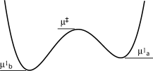
Figure 1: A continuum double-well potential that might underlie the two-state model. The fine-grained description follows particle trajectories over the continuum. The coarse-grained description is dominated by three chemical potentials: at the minima of the well (attracting fixed points) and the barrier maximum (the one-dimensional version of a saddle point).

1. The probability for a random walker to be found away from the attracting fixed points (the minima of the continuum free-energy potential) decreases exponentially in $\beta=1/k_{B}{\tt T}$, where ${\tt T}$ is temperature and $k_{B}$ is Boltzmann’s constant. In particular, escapes from one well to the other are exponentially improbable. The leading term in the log of the escape rate is given by the quasipotential of Freidlin-Wentzell theory Maier:escape:93 .

2. Among escape events, the majority occur along a particular spatio-temporal history of thermal excitations leading uphill from the minima of the potential toward the interior maximum. More precisely, conditional on having observed an escape event, the probability that the escape trajectory deviated from this most-probable form decreases exponentially in $\beta=1/k_{B}{\tt T}$, which is a large-deviations result for histories. The most-likely escape trajectory is the stationary path derived from the Freidlin-Wentzell dynamical system Maier:escape:93 . For one-dimensional systems, this trajectory is always the time-reverse of the classical diffusion trajectory from the maximum to the minimum.

3. The most-probable trajectory for any escape requires a specific finite time, which will limit the frequencies at which we can use coarse-grained approximations. In one dimension, the escape time equals the classical diffusive relaxation time over the path whose time-reverse is the escape.

The large-deviations scaling parameter in these continuum formulae is the inverse temperature $\beta=1/k_{B}{\tt T}$. $\beta$ will continue to be a scaling parameter in large-deviations formulae for the discrete approximation, but other parameters such as the number of random walkers in the system will also enter.

The exponential suppression of deviations from either fixed points or stereotypical escape trajectories is the phenomenon known as concentration of measure for the random walk in the potential. It is the property that leads us to make only a finite error even if we replace the infinitely many degrees of freedom of a random walk on the continuum, by a (zero-dimensional!) discrete random walk between two states, written

$$b\rightleftharpoons a.$$ (1)

Here $b$ and $a$ are coarse-grained labels standing for the left-hand and right-hand wells.

The states in the discrete walk are associated approximately with the positions of the local minima of the continuum potential, as shown in Fig. 2. Each state also has a Gibbs free energy per particle – known in chemical thermodynamics as the chemical potential Kittel:TP:80 , and written (for a single particle) as ${\mu}^{1}$ – near the value at the well minimum.

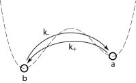
Figure 2: Discrete hops between well minima account for almost all structure in the probability distribution for the continuous random walk at low temperature. The role of the barrier potential (saddle point in Fig. 1) as the determiner of kinetics is absorbed in the transition rates $k_{\pm}$.

The continuum large-deviations theory for escapes Maier:escape:93 gives the escape rate from either well, to leading exponential order, as a function of the chemical potentials in the wells and at the local maximum of the continuum potential between the wells (indicated in Fig. 1), in the form

$$k_{+} = e^{-\beta\left({\mu}_{\ddagger}-{\mu}_{a}^{1}\right)},$$

$$k_{-} = e^{-\beta\left({\mu}_{\ddagger}-{\mu}_{b}^{1}\right)}.$$ (2)

Note that the absolute magnitudes of probabilities which are kept to describe transitions are generally (exponentially) smaller than corrections to the mean properties of the fixed points, which are omitted in the large-deviations approximation. They are, however, the leading terms in the conditional probability, and therefore the leading contribution to dynamics.

The escape rates appear in the discrete-state, continuous-time approximation as the parameters in its master equation, whose form is

$$\frac{\partial{\rho}_{{\rm n}_{a},{\rm n}_{b}}}{\partial t} = \left[k_{+}\left(e^{\partial/\partial{\rm n}_{a}-\partial/\partial{\rm n}_{b}}-1\right){\rm n}_{a}\right.$$ (3)

$$\mbox{}+\left.k_{-}\left(e^{\partial/\partial{\rm n}_{b}-\partial/\partial{\rm n}_{a}}-1\right){\rm n}_{b}\right]{\rho}_{{\rm n}_{a},{\rm n}_{b}}.$$

Here, ${\rm n}_{a}$ and ${\rm n}_{b}$ are possible values for the numbers of particles found in the right and left wells at any instant of time. ${\rho}_{{\rm n}_{a},{\rm n}_{b}}$ is a time-dependent probability density for an ensemble of such observations. The master equation (3) describes the flow of probability among different values of the indices $\left({\rm n}_{a},{\rm n}_{b}\right)$ as particles hop with rates $k_{\pm}$ per particle.

Often the right-hand side of a master equation such as Eq. (3) is written as a sum over all values of $\left({\rm n}_{a},{\rm n}_{b}\right)$. For stochastic processes in which almost all change results from independent single-particle transitions, only adjacent values $\left({\rm n}_{a}\pm 1,{\rm n}_{b}\mp 1\right)$ contribute to the change in ${\rho}_{{\rm n}_{a},{\rm n}_{b}}$. Therefore we have written the shifts of indices in the sum as the action of operators $e^{\partial/\partial{\rm n}_{b}-\partial/\partial{\rm n}_{a}}$, treating the indices $\left({\rm n}_{a},{\rm n}_{b}\right)$ formally as if they lived on a continuum, even though only values separated by integers ever appear in the time evolution of ${\rho}_{{\rm n}_{a},{\rm n}_{b}}$. The operator in square brackets in Eq. (3) is called the transfer matrix of the stochastic process. Its functional form will re-appear throughout the subsequent analyses, in the operators that govern the time evolution of generating functions, and as the Hamiltonian in the Freidlin-Wentzell dynamical system.

II.3 The discrete-state projections for equilibrium versus non-equilibrium systems

The net effect of concentration of measure in the continuum random walk is to extract the parameters of its discrete approximation from the fixed points of the mean flow on the free-energy landscape. The concentration toward the attracting fixed points is purely spatial, and is easy to visualize for landscapes in any number of dimensions. The concentration of escape trajectories is spatio-temporal, and is not directly illustrated in the static potential of Fig. 1. Concentration of trajectories takes on a spatial aspect for landscapes in more than one dimension, where transitions are exponentially likely to pass through saddle points, as shown in Fig. 3.

Figure 3: A Free energy landscape in more than one dimension, and its approximation by a discrete-state system. The charge-valued state variables of the equilibrium ensemble live at the attracting fixed points (black), where the principle axes of curvature (crosses) point in the same direction, so the scalar curvature of the landscape is positive. Current-valued state variables of the kinetic ensemble live on the saddle points (white), where principle axes of curvature point in opposite directions, and the scalar curvature is negative. Trajectories mostly sit at fixed points for long time intervals, but when transitions happen, they are exponentially likely to follow specific escape paths between basins, indicated by narrow curved paths.

We may now graphically characterize the difference between static and dynamic ensembles, for random walks on landscapes with basins and barriers. The equilibrium thermodynamic description for any such system is fully specified by the chemical potentials ${\mu}^{1}$ at the attracting fixed points (filled dots in Fig. 3). In this ensemble, there is no role for barriers, and no appearance of their chemical potentials ${\mu}^{\ddagger}$. The probabilities for state occupancy are determined only by their free energies, because all waiting times for escapes are (by assumption) surpassed.

For systems away from equilibrium, transition rates become essential to determining state occupancies, as well as transition frequencies between pairs of states. These rates are controlled by the saddle points (white dots in Fig. 3).

With each kind of fixed point we associate a state variable in the thermodynamic description. (See App. B for discussion of the origin and role of state variables as constraints.) The state variables of the equilibrium theory, which live on attracting fixed points, all have the property of charges: their value would not change if we ran the dynamics in time-reverse. Away from equilibrium, new state variables are introduced, which live on the saddle points, and these have the property of currents: their value would change sign if we ran the dynamics in time-reverse.

Non-equilibrium ensembles require the introduction of additional sets of current-valued state variables Smith:dual:05 ; Smith:DP:08 , which do not arise in equilibrium, and which have their origin in properties of the saddle points of the underlying free-energy landscape.

II.4 The nature of the local-equilibrium approximation

Free energy landscapes with basins and barriers lead to an extreme asymmetry in the way charge-valued and current-valued state variables are represented in the discrete model. The asymmetry comes, as noted above, from the fact that the leading probabilities for dynamics are exponentially smaller than corrections to the properties of states that are dropped in the large-deviations approximation. Therefore, in such systems, the charge-valued state variables, even in the non-equilibrium ensemble, are nearly identical to the state variables of equilibrium. The one-particle chemical potentials ${\mu}^{1}$, and their generalizations to concentration-dependent chemical potentials Kittel:TP:80 , all have the same relation to Gibbs free energy as in equilibrium. This property defines the local-equilibrium approximation for this class of models.

We note two things about the local-equilibrium approximation, to emphasize its limits. First, the equivalence of the non-equilibrium charge-valued state variables with their counterparts in equilibrium does not extend to the entropy Smith:dual:05 . The non-equilibrium entropy depends on both charges and currents, even at a single time. For ensembles of histories, it depends on the rate of transitions as well as the state-occupancy statistics, as we will show in multiple examples in Sec. IV and Sec. V. This fact will be essential to understanding “maximum-entropy production” Prigogine:MT:98 ; Dewar:FT_MEP:03 ; Dewar:MEP_NESM:04 ; Dewar:MEP_FT:05 ; Grinstein:MEP_error:07 as an approximation but not a principle for non-equilibrium systems.

Second, we note that the asymmetry between states and kinetics need not be a property of free energy landscapes if they do not have basins and barriers. In particular, it may not be a property of free diffusion, and it is generally not a property of driven dissipative quantum ensembles Smith:dual:05 . Therefore, if the underlying continuum model does not have the features that create asymmetry, we have no ground to expect that even the charge-valued state variables in the non-equilibrium theory will closely resemble those in the corresponding equilibrium limit.

II.5 The implicit “natural scale” for a coarse-grained description

Finally we mention an implicit limit on the use of the discrete-state approximation. Escapes in the continuum model are rare within the intervals that particles spend in either basin. However, they do require a non-zero time, comparable to the diffusive relaxation time. In the non-equilibrium discrete-state model, we will probe transition probabilities with time-dependent distortions of the chemical potentials ${\mu}^{1}$ and ${\mu}^{\ddagger}$. The model will permit these probes to have arbitrarily high-frequency time-dependence. However, we will see when we consider path entropies in Sec. V that such sources lead to divergences in individual entropy terms that should remain finite to be meaningful.

The solution to the problem of divergences is to recognize that the discrete model has a natural scale Polchinski:RGEL:84 , which is an upper bound on the frequencies that may sensibly appear in probes of the theory. The natural scale is the diffusive relaxation frequency in the continuum model. For probes with higher frequencies, the constants $k_{\pm}$ describing transition rates no longer retain their meaning or values. They were defined as lumped-parameter representations of escape paths, in a potential which was assumed to be fixed during the period of the escape. Faster probes “melt” the discrete approximation, and require that the description revert to the underlying continuum.

III Basic quantities introduced within the equilibrium ensemble: generating functions and the expressions of large-deviations scaling

We now begin the analysis of the equilibrium distribution for the two-state system. Since the entire equilibrium distribution may be written down analytically (it is a binomial distribution), the purpose of this “analysis” is to introduce the key quantities expressing large-deviations scaling, along with systematic ways to compute them using generating functions. The methods and the asymptotics will generalize immediately to time-dependent systems that are not exactly solvable, or at least very inconvenient to write in closed form.

The large-deviation result we will derive is that, for any apportionment $\left({\rm n}_{a},{\rm n}_{b}\right)$ of $N$ particles to the two states, the log-probability of this apportionment in the equilibrium distribution is the difference of the joint entropy from its maximizing value. A more extensive taxonomy of large-deviation results for equilibrium ensembles is given in Ref. Ellis:ELDSM:85 . Non-maximizing values of $\left({\rm n}_{a},{\rm n}_{b}\right)$ are termed fluctuations, and the relation between entropies and log-probability for sample values is therefore called a fluctuation theorem.

We will isolate this leading-exponential term in the log-probability by using the cumulant-generating function to shift the distribution, effectively projecting onto a sub-distribution within which $\left({\rm n}_{a},{\rm n}_{b}\right)$ is the most-likely value. The sub-distribution, when normalized, would be the equilibrium distribution in a two-state system with a shifted chemical potential; the ratio between the generating function and the normalized distribution measures the overlap of the original distribution with the one appropriate to $\left({\rm n}_{a},{\rm n}_{b}\right)$.

It will be the Legendre transform of this cumulant-generating function that gives the fluctuation probability to observe $\left({\rm n}_{a},{\rm n}_{b}\right)$ in the original equilibrium distribution, and expresses this probability as a difference of entropies. The Legendre transform of the cumulant-generating function is known, in some domains of quantum field theory, as the quantum effective action, and we will adapt that term here, calling it the “stochastic effective action”. (For more context and the relation to literature, see App. A.) Though it is only a difference of static entropies in the equilibrium ensemble, the stochastic effective action will become dynamical in ensembles of histories, where it will be the strict counterpart to the quantum effective action.

III.1 The equilibrium distribution of the two-state stochastic process

At an equilibrium steady state the solution to the master equation (3) is the binomial distribution

$${\rho}_{{\rm n}_{a},{\rm n}_{b}}^{\mbox{\scriptsize eq}} = \frac{k_{-}^{{\rm n}_{a}}k_{+}^{{\rm n}_{b}}}{{\left(k_{+}+k_{-}\right)}^{N}}\left(\begin{array}[]{c}N\\ {\rm n}_{a}\end{array}\right)$$ (6)

$$= {\bar{\nu}}_{a}^{{\rm n}_{a}}{\bar{\nu}}_{b}^{{\rm n}_{b}}\left(\begin{array}[]{c}N\\ {\rm n}_{a}\end{array}\right).$$ (9)

Total particle number $N={\rm n}_{a}+{\rm n}_{b}$ is conserved by all terms in the transfer matrix of Eq. (3). The equilibrium occupation fractions are

$${\bar{\nu}}_{a} \equiv \frac{k_{-}}{k_{+}+k_{-}}=\frac{e^{-\beta{\mu}_{a}^{1}}}{Z_{1}}$$

$${\bar{\nu}}_{b} \equiv \frac{k_{+}}{k_{+}+k_{-}}=\frac{e^{-\beta{\mu}_{b}^{1}}}{Z_{1}},$$ (10)

in which

$$Z_{1}\equiv e^{-\beta{\mu}_{a}^{1}}+e^{-\beta{\mu}_{b}^{1}}$$ (11)

is the called the partition function Kittel:TP:80 for a one-particle ensemble in this two-state system.

The Gibbs free energies for non-interacting particles scale linearly (that is, they are “extensive”) in particle number Kittel:TP:80 , so the structural terms in the large-deviations formulae for fluctuation probabilities will be functions of the ratios

$${\hat{\rm n}}_{a} \equiv \frac{{\rm n}_{a}}{N}$$

$${\hat{\rm n}}_{b} \equiv \frac{{\rm n}_{b}}{N}.$$ (12)

In both steady-state and time-dependent probability distributions, Roman ${\rm n}_{a}$, ${\rm n}_{b}$, ${\hat{\rm n}}_{a}$, ${\hat{\rm n}}_{b}$ will be used for discrete particle-number indices, respectively un-normalized or normalized by $N$. When the description of distributions is transferred to the generating function, the corresponding continuous indices will be $n_{a}$, $n_{b}$ for absolute number, and ${\nu}_{a}$, ${\nu}_{b}$ for relative numbers corresponding to the definitions (12).

For dynamical as for static systems, it is convenient to study open-system properties by considering an open system and its environment to be components in a larger closed system. Here the closed system will be defined by $N$ as a parameter, and we introduce the stochastic variable under the reaction ${\rm n}\equiv\left({\rm n}_{b}-{\rm n}_{a}\right)/2$, so that

$${\rm n}_{a} \equiv \frac{N}{2}-{\rm n}$$

$${\rm n}_{b} \equiv \frac{N}{2}+{\rm n}.$$ (13)

When only ${\rm n}$ is denoted explicitly, the distribution ${\rho}_{{\rm n}_{a},{\rm n}_{b}}$ will be indexed ${\rho}_{\rm n}$. The relative particle number asymmetry is likewise defined as ${\hat{\rm n}}\equiv\left({\hat{\rm n}}_{b}-{\hat{\rm n}}_{a}\right)/2$. Its counterpart in continuous variables will be denoted $\nu$. Equilibrium values for all numbers will be indicated with overbars.

The equilibrium distribution (9) may be cast in a variety of instructive forms. Using the relation (2) of the rate constants to one-particle chemical potentials, and Stirling’s formula for the logarithms of factorials, the following expressions re equivalent:

$${\rho}_{{\rm n}_{a},{\rm n}_{b}}^{\mbox{\scriptsize eq}} \approx \frac{1}{\sqrt{2\pi N{\hat{\rm n}}_{a}{\hat{\rm n}}_{b}}}e^{{\rm n}_{a}\left(\log{\bar{\hat{\rm n}}}_{a}-\log{\hat{\rm n}}_{a}\right)+{\rm n}_{b}\left(\log{\bar{\hat{\rm n}}}_{b}-\log{\hat{\rm n}}_{b}\right)}$$ (14)

$$\equiv \frac{1}{\sqrt{2\pi N{\hat{\rm n}}_{a}{\hat{\rm n}}_{b}}}e^{-ND\left(\hat{\rm n}\parallel{\bar{\hat{\rm n}}}\right)}$$

$$= \frac{1}{\sqrt{2\pi N{\hat{\rm n}}_{a}{\hat{\rm n}}_{b}}}\frac{1}{Z_{1}^{N}}e^{-\beta{\rm n}_{a}\left({\mu}_{a}^{1}+\tau\log{\hat{\rm n}}_{a}\right)-\beta{\rm n}_{b}\left({\mu}_{b}^{1}+\tau\log{\hat{\rm n}}_{b}\right)}$$

$$= \frac{1}{\sqrt{2\pi N{\hat{\rm n}}_{a}{\hat{\rm n}}_{b}}}e^{N\log\left(N/Z_{1}\right)}e^{-\beta{\rm n}_{a}{\mu}_{a}-\beta{\rm n}_{b}{\mu}_{b}}$$

$$= e^{N\log\left(N/Z_{1}\right)}\sqrt{\frac{{\rm n}_{a}+{\rm n}_{b}}{2\pi{\rm n}_{a}{\rm n}_{b}}}e^{-\beta\left(G_{a}+G_{b}\right)}$$

In the second line, $D\!\left(\hat{\rm n}\parallel{\bar{\hat{\rm n}}}\right)$ is the Kullback-Leibler divergence Cover:EIT:91 , in which $\hat{\rm n}$ and $\bar{\hat{\rm n}}$ stand for the distributions with coefficients $\left({\hat{\rm n}}_{a},{\hat{\rm n}}_{b}\right)$, $\left({\bar{\hat{\rm n}}}_{a},{\bar{\hat{\rm n}}}_{b}\right)$ respectively. The ${\rm n}_{a}$- and ${\rm n}_{b}$-particle chemical potentials add concentration corrections to the entropy in the one-particle potentials, as

$${\mu}_{a} = {\mu}_{a}^{1}+k_{B}{\tt T}\log{\rm n}_{a}$$

$${\mu}_{b} = {\mu}_{b}^{1}+k_{B}{\tt T}\log{\rm n}_{b}.$$ (15)

By comparing the second with the last-two lines of Eq. (14), we see that the minimum of the Gibbs free energies of the subsystems over ${\rm n}$ is

$$\beta\min_{\rm n}\!\left[G_{a}+G_{b}\right]\equiv\beta\min\!\left[{\rm n}_{a}{\mu}_{a}+{\rm n}_{b}{\mu}_{b}\right]=N\log\frac{N}{Z_{1}}.$$ (16)

The one-particle minimum expressed in terms of fractional occupancies, which is the descaled version at any $N$, gives an $N$-independent relation between the chemical potential per particle, and the one-particle partition function,

$$\min_{\hat{\rm n}}\!\left[{\hat{\rm n}}_{a}\left({\mu}_{a}^{1}+k_{B}{\tt T}\log{\hat{\rm n}}_{a}\right)+{\hat{\rm n}}_{b}\left({\mu}_{b}^{1}+k_{B}{\tt T}\log{\hat{\rm n}}_{b}\right)\right]$$ (17)

$$= -k_{B}{\tt T}\log Z_{1}.\phantom{k_{B}{\tt T}\log Z_{1}k_{B}{\tt T}\log Z_{1}k_{B}{\tt T}\log Z_{1}}$$

These are the standard relations for ideal gases or dilute solutions.

III.1.1 The aggregation of state variables and the fluctuation probability

The local-equilibrium approximation for the two-state system allows us to approximate the log-probabilities for non-equilibrium configurations of $\left({\rm n}_{a},{\rm n}_{b}\right)$ by the sum of free energies for the individual wells. At the minimizing value of $\left({\rm n}_{a},{\rm n}_{b}\right)$ for this sum, the equilibrium free energy for the composite system is attained. We may therefore express the minimum joint free energy per particle, using Eq. (16), as a definition for the single-particle chemical potential for the equilibrated system, in a form equivalent to to Eq. (15):

$$\frac{1}{N}\min\!\left[G_{a}+G_{b}\right]\equiv{\mu}_{a\cup b} = -k_{B}{\tt T}\log Z_{1}+k_{B}{\tt T}\log N$$ (18)

$$\equiv {\mu}_{a\cup b}^{1}+k_{B}{\tt T}\log N.$$

Here ${\mu}_{a\cup b}^{1}$ is the whole-system counterpart to the one-particle chemical potentials ${\mu}_{a}^{1}$ and ${\mu}_{b}^{1}$ for subsystems in the local-equilibrium approximation.

The density values in the equilibrium distribution (14) may then be written as exponentials of the $\left(\mbox{system}+\mbox{environment}\right)$ entropies of Eq. (176), as

$${\rho}_{{\rm n}_{a},{\rm n}_{b}}^{\mbox{\scriptsize eq}} \approx e^{\beta N{\mu}_{a\cup b}}\sqrt{\frac{{\rm n}_{a}+{\rm n}_{b}}{2\pi{\rm n}_{a}{\rm n}_{b}}}e^{-\beta\left(G_{a}+G_{b}\right)}$$ (19)

$$\approx e^{\beta G_{a\cup b}}\sqrt{\frac{{\rm n}_{a}+{\rm n}_{b}}{2\pi{\rm n}_{a}{\rm n}_{b}}}e^{-\beta\left(G_{a}+G_{b}\right)}.$$

As explained in App. B, all three Gibbs free energies are functions of intensive $k_{B}{\tt T}$ and $p$, and of extensive arguments ${\rm n}_{a}$, ${\rm n}_{b}$, and $N$. Since total energy is controlled by the environment temperature, it is the entropy components of these $G$ values for the subsystems, as functions of ${\rm n}_{a}$ and ${\rm n}_{b}$, which control the difference of $G_{a}+G_{b}$ from $G_{a\cup b}$.

III.1.2 Entropies of equilibrium and residual fluctuations

The leading-exponential approximation of large-deviations scaling separates extensive entropies of the subsystems, which were defined into the parameters of the two-state stochastic process from coarse-graining the continuum model, from entropies due to chemical fluctuation, which are sub-extensive. To see this, following any standard thermodynamics text Kittel:TP:80 , we write any of the one-particle chemical potentials ${\mu}^{1}\equiv h^{1}-k_{B}{\tt T}s^{1}$, in which $h^{1}$ is the specific enthalpy and $s^{1}$ is the specific entropy. This decomposition yields a relation between subsystem and whole system free energies at equilibrium, which is

$$h^{1}_{a\cup b} = {\bar{\hat{\rm n}}}_{a}h^{1}_{a}+{\bar{\hat{\rm n}}}_{b}h^{1}_{b}$$

$$s^{1}_{a\cup b} = {\bar{\hat{\rm n}}}_{a}s^{1}_{a}+{\bar{\hat{\rm n}}}_{b}s^{1}_{b}-{\bar{\hat{\rm n}}}_{a}\log{\bar{\hat{\rm n}}}_{a}-{\bar{\hat{\rm n}}}_{b}\log{\bar{\hat{\rm n}}}_{b}.$$ (20)

The free energy in the thermodynamic limit is then given by

$$G_{a\cup b}=N\left(h^{1}_{a\cup b}-k_{B}{\tt T}s^{1}_{a\cup b}+k_{B}{\tt T}\log N\right),$$ (21)

which extensive in particle number, if we think of the $\log N$ term as being set by pressure. In comparison, the Shannon entropy of the full distribution over fluctuations contains a term from the normalization of the exponential in Eq. (19), due to its width,

$$-\sum_{\rm n}{\rho}_{\rm n}^{\mbox{\scriptsize eq}}\log{\rho}_{\rm n}^{\mbox{\scriptsize eq}}\approx\frac{1}{2}\left[1+\log\left(2\pi N{\bar{\hat{\rm n}}}_{a}{\bar{\hat{\rm n}}}_{b}\right)\right].$$ (22)

This correction, being only logarithmic, is sub-extensive in $N$.

III.2 Generating functions and the stochastic effective action

A moment-generating function – or “ordinary power-series generating function” Wilf:gen_fun:06 – for a distribution indexed on the two numbers ${\rm n}_{a}$ and ${\rm n}_{b}$ has two complex arguments, and is written

$$\psi\!\left(z_{a},z_{b}\right)\equiv\sum_{{\rm n}_{a},{\rm n}_{b}}z_{a}^{{\rm n}_{a}}z_{b}^{{\rm n}_{b}}{\rho}_{{\rm n}_{a},{\rm n}_{b}}.$$ (23)

To study the properties of ${\rho}_{\rm n}$ at fixed $N$, recognizing that $z_{a}^{{\rm n}_{a}}z_{b}^{{\rm n}_{a}}={\left(z_{a}z_{b}\right)}^{N/2}{\left(z_{b}/z_{a}\right)}^{\rm n}$, we may set $z_{a}z_{b}\equiv 1$ and denote $z_{b}/z_{a}\equiv z$. At equilibrium we will be interested only in the one-argument function of $z$. However, as we pass to dynamical descriptions, it will remain convenient in some cases to retain both variables $z_{a}$ and $z_{b}$, even if they are applied to a distribution with support on only one value of $N$.

The weight factors $z^{\rm n}$ have an effect similar to shift in the subsystem chemical potentials, which will recur repeatedly in our analysis. Therefore we denote $z=e^{q}$, and write the one-variable generating function as

$$\psi\!\left(z\right) = \sum_{\rm n}z^{\rm n}{\rho}_{\rm n}^{\mbox{\scriptsize eq}}$$ (26)

$$= \sum_{\rm n}{\left({\bar{\hat{\rm n}}}_{a}/\sqrt{z}\right)}^{{\rm n}_{a}}{\left({\bar{\hat{\rm n}}}_{b}\sqrt{z}\right)}^{{\rm n}_{b}}\left(\begin{array}[]{c}N\\ {\rm n}_{a}\end{array}\right)$$

$$= {\left(\frac{Z_{1}^{\left(q\right)}}{Z_{1}}\right)}^{N}\sum_{\rm n}{\tilde{\hat{\rm n}}}_{a}^{{\rm n}_{a}}{\tilde{\hat{\rm n}}}_{b}^{{\rm n}_{b}}\left(\begin{array}[]{c}N\\ {\rm n}_{a}\end{array}\right).$$ (29)

Here new normalized fractions in the presence of $q$ – which will be referred to as a source – are defined by

$${\tilde{\hat{\rm n}}}_{a} \equiv \frac{{\bar{\hat{\rm n}}}_{a}e^{-q/2}}{{\bar{\hat{\rm n}}}_{a}e^{-q/2}+{\bar{\hat{\rm n}}}_{b}e^{q/2}}=\frac{e^{-\left(\beta{\mu}_{a}^{1}+q/2\right)}}{Z_{1}^{\left(q\right)}}$$

$${\tilde{\hat{\rm n}}}_{b} \equiv \frac{{\bar{\hat{\rm n}}}_{b}e^{q/2}}{{\bar{\hat{\rm n}}}_{a}e^{-q/2}+{\bar{\hat{\rm n}}}_{b}e^{q/2}}=\frac{e^{-\left(\beta{\mu}_{b}^{1}-q/2\right)}}{Z_{1}^{\left(q\right)}},$$ (30)

and the associated one-particle partition function with source $q$ is

$$Z_{1}^{\left(q\right)}\equiv e^{-\left(\beta{\mu}_{a}^{1}+q/2\right)}+e^{-\left(\beta{\mu}_{b}^{1}-q/2\right)}.$$ (31)

The sum in the third line of Eq. (29) evaluates to unity, as for any normalized binomial, but it is instructive to use what was learned in forming Eq. (19) to recast the sum and prefactor together in terms of a normalized distribution and a “penalty” term, as

$$\psi\!\left(z\right)\approx e^{\beta G_{a\cup b}-\beta G_{a\cup b}^{\left(q\right)}}\sum_{\rm n}e^{\beta G_{a\cup b}^{\left(q\right)}}\sqrt{\frac{{\rm n}_{a}+{\rm n}_{b}}{2\pi{\rm n}_{a}{\rm n}_{b}}}e^{-\beta\left(G_{a}^{\left(q\right)}+G_{b}^{\left(q\right)}\right)}$$ (32)

In Eq. (32) the subsystem free energies are defined at any ${\rm n}_{a}$, ${\rm n}_{b}$ as

$$G_{a}^{\left(q\right)} = G_{a}+{\rm n}_{a}k_{B}{\tt T}q/2$$

$$G_{b}^{\left(q\right)} = G_{b}-{\rm n}_{b}k_{B}{\tt T}q/2.$$ (33)

We wish to introduce $G_{a\cup b}^{\left(q\right)}$ as the minimum of $G_{a}^{\left(q\right)}+G_{b}^{\left(q\right)}$ over ${\rm n}$, as before. However, for discrete ${\rm n}$, this gives a discontinuous function of $q$. The thermodynamic usage of $G_{a\cup b}^{\left(q\right)}$ is as a macroscopic function of its intensive state variables, and therefore it will save intermediate steps and notation simply to define $G_{a\cup b}^{\left(q\right)}$ as the minimum over ${\rm n}$ treated as a continuous variable, whose minimizing argument will then be a continuous function of $q$.

For such binomial distributions or their multinomial generalizations, sources of the form $k_{B}{\tt T}q=q/\beta$ behave as shifts in chemical potential, in this case split evenly between subsystems $a$ and $b$. The “penalty” term is expressed as a function of $\left(G_{a\cup b}-G_{a\cup b}^{\left(q\right)}\right)$: the minimum chemical work needed to convert the system with potential difference ${\mu}_{b}-{\mu}_{a}$ and equilibrium $\bar{\hat{\rm n}}$ to one with potential difference ${\mu}_{b}-{\mu}_{a}-q/\beta$ and an equilibrium ${\bar{\hat{\rm n}}}^{\left(q\right)}$ determined by the new potentials. $\beta\left(G_{a\cup b}-G_{a\cup b}^{\left(q\right)}\right)$ is also the log-probability to obtain the shifted distribution from the original through the set of weights $z^{\rm n}$.

The penalty function is referred to as the cumulant-generating function and denoted $\Gamma\!\left(q\right)$. It is defined from the moment-generating function $\psi$ by the relation

$$\psi\!\left(z\right)\equiv e^{-\Gamma\left(\log z\right)}=e^{-\Gamma\left(q\right)}.$$ (34)

From the definition (29) of the moment-generating function it follows that

$$\frac{d\log\psi\!\left(z\right)}{d\log z}=-\frac{d\Gamma\!\left(q\right)}{dq}={\left<{\rm n}\right>}^{\left(q\right)}\equiv n^{\left(q\right)},$$ (35)

in which we introduce the continuous counterpart $n^{\left(q\right)}$ as both the gradient of $\Gamma$ and the expectation of ${\rm n}$ under the equilibrium distribution shifted by $z$.

From Eq. (32), the cumulant-generating function is just the Gibbs free energy difference

$$\Gamma\!\left(q\right)=\beta G_{a\cup b}^{\left(q\right)}-\beta G_{a\cup b}.$$ (36)

Recasting Eq. (35),

$$-\frac{d\Gamma\!\left(q\right)}{dq}=\frac{dG_{a\cup b}^{\left(q\right)}}{d\left(-k_{B}{\tt T}q\right)}=n^{\left(q\right)},$$ (37)

we recover the usual relation from equilibrium thermodynamics Kittel:TP:80 , that the gradient of the Gibbs free energy with respect to the chemical potential is the particle number.

For reference in later sections, we may compute closed forms for the various quantities. Define $\bar{\mu}\equiv{\mu}_{b}^{1}-{\mu}_{a}^{1}$, dual to the relative particle-number difference $\bar{\hat{\rm n}}$. Then

$$n^{\left(q\right)}=\frac{N}{2}\tanh\frac{1}{2}\left(q-\beta\bar{\mu}\right),$$ (38)

and

$$\Gamma\!\left(q\right)=N\left[\log\cosh\frac{\beta\bar{\mu}}{2}-\log\cosh\frac{1}{2}\left(q-\beta\bar{\mu}\right)\right].$$ (39)

In continuum field theories with many particles and nonlinear interactions among them, it is often necessary to approximate the moment- and cumulant-generating functions by series expansions in the variance of the Gaussian approximation to fluctuations. In such an expansion, The gradient of $\Gamma$ yields all of the connected graphs giving $n^{\left(q\right)}$, while the gradient of $\psi$ gives a sum over all graphs (see Ref. Weinberg:QTF_II:96 Ch. 16).

III.2.1 The stochastic effective action for single-time fluctuations

App B reviews the fact that the Gibbs free energy is a Legendre transform of the entropy. Thus, the entropy is the converse Legendre transform of the Gibbs free energy. We may therefore expect that by Legendre transforming $\Gamma\!\left(q\right)$, we will arrive at a direct expression for the entropy differences that govern internal fluctuations of particle number, without reference to external temperature or pressure.

The Legendre transform of the cumulant generating function $\Gamma$ is known as an effective action Weinberg:QTF_II:96 . When it is computed for the single-time binomial distribution, it hardly seems to justify its name, if we expect an action in the sense of Hamiltonian dynamics. However, it will become just such an action in the time-dependent ensemble. Here we introduce the Legendre transform for its statistical meaning, and later we introduce the dynamical version.

The definition is

$$S^{\mbox{\scriptsize eff}}\!\left(n\right)\equiv{\left.\left[\Gamma\!\left(q\right)+nq\right]\right|}_{q=q^{\left(n\right)}},$$ (40)

in which $q^{\left(n\right)}$ denotes the inverse function of $n^{\left(q\right)}$ from Eq. (37).  From the gradient relation (35) it follows that

$$\frac{dS^{\mbox{\scriptsize eff}}\!\left(n\right)}{dn}=q^{\left(n\right)}.$$ (41)

Therefore $S^{\mbox{\scriptsize eff}}$ must vanish at the mean value of ${\rm n}$ in the distribution $\rho$ for which it is computed, because no source (i.e., $q\!\left(n\right)=0$) is required to yield the equilibrium value as the mean.

Addition of the term $n^{\left(q\right)}q$ to $\Gamma$ in Eq. (40) cancels only the explicit $q/\beta$ term in the shifted free energy $G_{a\cup b}^{\left(q\right)}$, leaving the particle assignments $n_{a}^{\left(q\right)},n_{b}^{\left(q\right)}$ unchanged. The terms that remain are precisely those in the fluctuation theorem: they are the subsystem free energies evaluated at shifted $n$s. The effective action may be written

$$S^{\mbox{\scriptsize eff}}\!\left(n\right)=\beta G_{a}\!\left(n_{a}\right)+\beta G_{b}\!\left(n_{b}\right)-\beta G_{a\cup b}\!\left(N\right).$$ (42)

In Eq. (42) the free energies $G$ are now regarded as functions of the continuous-valued $n_{a}$ and $n_{b}$ rather than the discrete indices ${\rm n}_{a}$ and ${\rm n}_{b}$ on which the distribution is defined.

Referring back to the distribution over fluctuations in the original ${\rho}_{n_{s},n_{p}}^{\mbox{\scriptsize eq}}$ of Eq. (19), we see that $\exp\!\left(-S^{\mbox{\scriptsize eff}}\right)$ directly extracts the leading exponential dependence of the fluctuation probability. It omits sub-extensive normalization factors related to the width of the distribution. Therefore the effective action directly expresses the large-deviations scaling for fluctuation probabilities. The log-probability approximated by Eq. (42) scales linearly in $N$, and its structure is determined by the remaining $N$-invariant fractions ${\nu}_{a}$ and ${\nu}_{b}$.

For reference in comparison to later expressions for the effective actions of fluctuating histories, the effective action for the equilibrium distribution evaluates to

$$S^{\mbox{\scriptsize eff}}\!\left(n\right) = N\left[\log\cosh\frac{\beta\bar{\mu}}{2}-\log\cosh\frac{1}{2}\left(q^{\left(n\right)}-\beta\bar{\mu}\right)\right.$$ (43)

$$\mbox{}+\left.\frac{q^{\left(n\right)}}{2}\tanh\frac{1}{2}\left(q^{\left(n\right)}-\beta\bar{\mu}\right)\right],$$

in which $q^{\left(n\right)}$ is evaluated by inversion of Eq. (38).

IV Ensemble of histories I: the master equation for number; Doi-Peliti construction of the generating functional; the dynamical-system representation of Freidlin and Wentzell

We now construct a second generating function and ensemble, for the time-dependent distribution $\rho$ evolving under the master equation (3), rather than merely for its equilibrium steady state. The equilibrium fluctuation results of Sec. III will reappear within this larger construction, as probabilities for histories conditioned on their behavior at a single instant but on no other information. Here, however, the single-time fluctuation probabilities will no longer be computed as primitive quantities. Instead, they will arise as integrals of log-probability along the entire histories which are most-likely, conditioned on achieving a particular deviation at a single time.

In keeping with the shift from states to histories, the cumulant-generating function and effective action in this section will be functionals, whose arguments are sequences of occupation numbers $\left({\rm n}_{a},{\rm n}_{b}\right)$. The description derived from the master equation will still only count particle numbers, and will not resolve identities. Unlike the equilibrium constructions, the path-space large-deviations formulae will not allow us to identify the natural path-entropy functions, for which we will require the caliber formulation of Sec. V. However, this section will introduce the remarkable Freidlin-Wentzell formulation of large-deviations theory as a Hamiltonian dynamical system, in which the stochastic effective action will become a genuine Lagrange-Hamilton action functional.

IV.1 Liouville time evolution and the coherent-state expansion for its quadrature

The reason to study generating functions at equilibrium is that the moments of the equilibrium distribution may be more relevant and robust descriptions of fluctuations than individual probability values ${\rho}_{{\rm n}_{a},{\rm n}_{b}}$. Similarly, the reason to use generating functions to study dynamics is that the basis of single-particle hops is often less informative than a basis in the collective motions of many particles.

The master equation formalism acts on probabilities in the basis of single-particle hops. The counterpart, which acts on the moment-generating function, is known as a Liouville equation. When specified in complete detail, the Liouville equation has the same information as its corresponding master equation. However, low-order approximations to the Liouville form will often contain more of the total information than similarly reduced approximations in the basis of single-particle hops. Such approximations are sometimes called the hydrodynamic limit Gaspard:rev_entropy:04 . Therefore the Liouville form is the starting point for methods of Gaussian integration, Langevin equations, or other commonly used approximation schemes.

IV.1.1 The master equation expressed as a function of mass-action rates

The two-state master equation (3) is an instance of a wider class of equations describing single-particle exchanges. A notation for the more general class is introduced here, both because it cleanly divides the particle-hopping terms associated with stochasticity from the probabilities which coincide with mass-action rates, and because it immediately generalizes to more complex reaction stoichiometries, such as those required by chemical reaction networks. The master equation for the two-state system is written in this general form as

$$\frac{\partial{\rho}_{\vec{{\rm n}}}}{\partial t}=\sum_{i,j\in\left\{a,b\right\}}\left(e^{\partial/\partial{\rm n}_{i}-\partial/\partial{\rm n}_{j}}-1\right)r_{ji}{\rho}_{\vec{{\rm n}}}.$$ (44)

Here $\vec{\rm n}$ is a vector whose components give the number of particles of each type $i\in 1,\ldots,I$ (here $\vec{\rm n}=\left({\rm n}_{a},{\rm n}_{b}\right)$). For the linear reaction model, the mass-action rates $r_{ji}$

$$r_{ba} = k_{+}{\rm n}_{a}$$

$$r_{ab} = k_{-}{\rm n}_{b}$$ (45)

describe the probability for particle transfer from state $i$ to state $j$. The form (44) extends immediately to arbitrary many-particle exchanges with rates that may involve powers of many different components of $\vec{\rm n}$, and to arbitrary network connections. The general methods derived below extend immediately to all those cases. Even the shortcuts we will introduce, to pass directly from the form of the master equation to the action functional of Freidlin-Wentzell theory, apply with no changes.

IV.1.2 Definition of the Liouville operator from the transfer matrix

This section sketches the conversion from number terms and index shifts in the master equation, to the equivalent polynomials and differential operators in the Liouville equation. It then converts the representation on polynomials to the representation introduced by Masao Doi Doi:SecQuant:76 ; Doi:RDQFT:76 , in terms of raising and lowering operators in an abstract linear vector space. The systematic construction of Liouville forms from master equations is now standard Eyink:action:96 ; Mattis:RDQFT:98 , and its form for the linear mass-action kinetics of Eq. (45) is the simplest possible.

In the vector notation, the generating function at a single time becomes a function of a vector $\vec{z}$ whose components correspond to those of $\vec{\rm n}$. Here the moment-generating function is

$$\psi\!\left(\vec{z}\right)=\sum_{\vec{{\rm n}}}\prod_{i\in\left\{a,b\right\}}z_{i}^{{\rm n}_{i}}{\rho}_{\vec{{\rm n}}}.$$ (46)

Time evolution under Eq. (44) implies time evolution of $\psi$ according to

$$\frac{\partial\psi\!\left(\vec{z}\right)}{\partial t} = \sum_{\vec{{\rm n}}}\prod_{k\in\left\{a,b\right\}}z_{k}^{{\rm n}_{k}}\frac{\partial{\rho}_{\vec{{\rm n}}}}{\partial t}$$ (47)

$$= \sum_{i,j\in\left\{a,b\right\}}\left(\frac{z_{j}}{z_{i}}-1\right)\sum_{\vec{{\rm n}}}\prod_{k\in\left\{a,b\right\}}z_{k}^{{\rm n}_{k}}r_{ji}\!\left({\rm n}_{i}\right){\rho}_{\vec{{\rm n}}},$$

$$= \sum_{i,j\in\left\{a,b\right\}}\left(\frac{z_{j}}{z_{i}}-1\right)r_{ji}\!\left(z_{i}\frac{\partial}{\partial z_{i}}\right)\sum_{\vec{{\rm n}}}\prod_{k\in\left\{a,b\right\}}z_{k}^{{\rm n}_{k}}{\rho}_{\vec{{\rm n}}},$$

$$\equiv -\mathcal{L}\!\left(\vec{z},\frac{\partial}{\partial\vec{z}}\right)\psi\!\left(\vec{z}\right).$$

Here we have written out the functional dependence of $r_{ij}$ on the number indices of the particle species entering half-reactions explicitly, to show how those number indices are replaced by products $z_{i}\partial/\partial z_{i}$ acting on the basis polynomials of the generating function. Successive lines of Eq. (47) reflect the action of successive terms in the master equation (44). The extension of these steps to multi-species reactions also follows a standard form Mattis:RDQFT:98 , of which our example is representative. The differential operator $\mathcal{L}\!\left(\vec{z},\partial/\partial\vec{z}\right)$ is the Liouville operator for this stochastic process.

Time evolution of the density ${\rho}_{\vec{n}}$ over an interval $\left[0,T\right]$ is performed by taking the quadrature of Eq. (47), which we may think of as being performed over a sequence of short time intervals of length $\delta t$:

$${\psi}_{T} = \mathcal{T}e^{\int_{0}^{T}dt\,\mathcal{L}}{\psi}_{0}$$ (48)

$$= \mathcal{T}\prod_{k=1}^{T/\delta t}e^{\delta t\,\mathcal{L}}{\psi}_{0}.$$

$\mathcal{T}$ denotes time-ordering in the product, and we will use the same notation when the product of exponential terms $e^{\delta t\,\mathcal{L}}$ is written as the exponential of a sum or integral. Such expressions are known as time-ordered exponential integrals. For the Liouville operator with constant coefficients, time-ordering serves no explicit purpose, but when time-dependent sources are introduced below, it will become necessary.

We may efficiently approximate the product (48) by interposing a complete distribution of generating functions between each of the small increments of time evolution in the second line, which we develop in the next sub-section. Doing so, however, introduces a distinct set of arguments $\vec{z}$ at each time, which are cumbersome to work with. Therefore, at intermediate times between $0$ and $T$, it is conventional to adopt an abstract notation for the complex vectors and derivatives Doi:SecQuant:76 ; Doi:RDQFT:76 , which more clearly reflect the nature of the generating function as a vector in a normed linear space (a Hilbert space). The correspondence of the elementary monomials,

$$z_{j} \leftrightarrow a_{j}^{\dagger},$$ (49)

$$\frac{\partial}{\partial z_{i}} \leftrightarrow a^{i},$$ (50)

reflects the property that complex variables and their derivatives satisfy the algebra of raising and lowering operators familiar from the quantum harmonic oscillator,

$$\left[\frac{\partial}{\partial z_{i}},z_{j}\right]\leftrightarrow\left[a^{i},a_{j}^{\dagger}\right]={\delta}^{i}_{j}.$$ (51)

Polynomials built from these variables live in a function space built on a “vacuum” which is simply the number 1, denoted

$$1\leftrightarrow\left|0\right).$$ (52)

The conjugate operation to creating a generating function is the evaluation of the trace – generally with moment-sampling operators to extract its moments – so that the conjugate operator to the right-hand vacuum (52) is an integral,

$$\int d^{I}\!z\,\delta\!\left(z\right)\leftrightarrow\left(0\right|.$$ (53)

From these definitions an entire function space with inner product can be built up, as reviewed in Ref’s. Mattis:RDQFT:98 ; Cardy:FTNEqSM:99 .

IV.1.3 The coherent-state expansion

The transformation from discrete number-states to generating functions is the Laplace transform. It may be applied within the discrete time slices of the quadrature (48), where it makes use of the Laplace transforms of intermediate Poisson distributions, which are known as coherent states. It has become conventional in the Doi-Peliti literature to denote the mean values of these Poisson distributions with the field $\phi$; for a multi-state system, we index them with a complex-valued vector field $\vec{\phi}$. The conjugate vectors to these Poisson distributions are moment-sampling operators, weighted by Hermitian conjugate field variables denoted ${\vec{\phi}}^{\dagger}$.

The ${\vec{\phi}}^{\dagger}$ will have the property that, dynamically, they propagate information backward in time from final data imposed by the weights $z_{a}$, $z_{b}$. The interpretation of this property is that the moment-sampling operators capture conditional distributions at earlier times, conditioned on the final values they produce. The fields $\vec{\phi}$ and ${\vec{\phi}}^{\dagger}$ will turn out to be the position fields and their conjugate-momentum fields in one version of the Freidlin-Wentzell theory, and the Hamiltonian under which they evolve will be the Liouville operator. The way evolution under the dynamical system is made consistent with the “backward” propagation of information, by the conjugate momentum, is that the momentum variables will typically have unstable evolution forward in time, while the position variables will evolve in stable directions.

In this section we construct the coherent-state expansion for the quadrature (48), which is due to Peliti Peliti:PIBD:85 ; Peliti:AAZero:86 .

The Liouville operator is a function of raising and lowering operators $\left\{a^{i}\right\}$, $\left\{a^{\dagger}_{j}\right\}$ so the convenient expansion of Eq. (48) will be given by a basis of eigenstates of these operators. The coherent states are constructed to be such eigenstates. The right-hand coherent state is defined as

$$\left|\vec{\phi}\right) = e^{-\left({\vec{\phi}}^{\dagger}\cdot\vec{\phi}\right)/2}e^{{\vec{a}}^{\dagger}\cdot\vec{\phi}}\left|0\right)$$ (54)

$$= e^{-\left({\vec{\phi}}^{\dagger}\cdot\vec{\phi}\right)/2}\sum_{M=0}^{\infty}\frac{{\left({\vec{a}}^{\dagger}\cdot\vec{\phi}\right)}^{M}}{M!}\left|0\right)$$

$$= \prod_{m=1}^{I}\left(e^{-\left({\phi}_{m}^{\dagger}{\phi}_{m}\right)/2}\sum_{n_{m}=0}^{\infty}\frac{{\phi}_{m}^{n_{m}}}{n_{m}!}{a_{m}^{\dagger}}^{n_{m}}\right)\left|0\right).$$

The components of its complex parameter vector $\vec{\phi}$ correspond to those of $\vec{z}$. From the commutator algebra (51), and the fact that all $a^{i}\leftrightarrow\partial/\partial z_{i}$ annihilate the right vacuum (52), it follows that Eq. (54) does define an eigenstate of all the lowering operators $a^{i}$ with corresponding eigenvalues ${\phi}^{i}$,

$$a^{i}\left|\vec{\phi}\right)={\phi}^{i}\left|\vec{\phi}\right).$$ (55)

The left-hand coherent state dual to Eq. (54) is given by

$$\left({\vec{\phi}}^{\dagger}\right| = \left(0\right|e^{{\vec{\phi}}^{\dagger}\cdot\vec{a}}e^{-\left({\vec{\phi}}^{\dagger}\cdot\vec{\phi}\right)/2}$$ (56)

$$= \left(0\right|\sum_{M=0}^{\infty}\frac{{\left({\vec{\phi}}^{\dagger}\cdot\vec{a}\right)}^{M}}{M!}e^{-\left({\vec{\phi}}^{\dagger}\cdot\vec{\phi}\right)/2}.$$

Eq. (56) is likewise checked to be an eigenstate of the raising operators, with eigenvalues ${\phi}_{j}^{\dagger}$,

$$\left({\vec{\phi}}^{\dagger}\right|a_{j}^{\dagger}=\left({\vec{\phi}}^{\dagger}\right|{\phi}_{j}^{\dagger}.$$ (57)

The presence of $\vec{a}$ corresponding to $\partial/\partial\vec{z}$ in Eq. (56) gives the left-hand coherent state the interpretation of a moment-sampling operator. This state displaces any argument $a^{\dagger}_{j}$ in the state that it acts on (through the inner product), by a summand ${\phi}^{\dagger}_{j}$. It then sets the original $a^{\dagger}_{j}$ to zero because all left-hand states include the trace defined by the left vacuum (53).

The sum of outer products of a left-hand coherent state and its dual right-hand coherent state gives a representation of the identity operator as an over-complete integral over states,

$$\int\frac{d^{I}\!{\phi}^{\dagger}d^{I}\!\phi}{{\pi}^{I}}\left|\vec{\phi}\right)\left({\vec{\phi}}^{\dagger}\right|=I.$$ (58)

The result of taking the inner product of Eq. (58) with any state $\left|\vec{\psi}\right)$ on the right is that the moment-sampling operator $\left({\vec{\phi}}^{\dagger}\right|$ simply transposes the weights that it extracts from$\left|\vec{\psi}\right)$onto the left-coherent states $\left|\vec{\phi}\right)$ in the expansion (58).

If we insert a complete set of states in this form between every term in the product (48), we express the moment-generating function at time $T$ as an integral over all intermediate values of the field variables $\vec{\phi}$, ${\vec{\phi}}^{\dagger}$, of the form

$$\psi\!\left(z_{a},z_{b}\right)\equiv e^{-{\Gamma}_{T}\left(\log z_{a},\log z_{b}\right)}=\int_{0}^{T}\mathcal{D}{\phi}^{\dagger}_{a}\mathcal{D}{\phi}_{a}\mathcal{D}{\phi}^{\dagger}_{b}\mathcal{D}{\phi}_{b}e^{\left(z_{a}-{{\phi}^{\dagger}_{a}}_{T}\right){{\phi}_{a}}_{T}+\left(z_{b}-{{\phi}^{\dagger}_{b}}_{T}\right){{\phi}_{b}}_{T}-S-{\Gamma}_{0}\left(\log{{\phi}^{\dagger}_{a}}_{0},\log{{\phi}^{\dagger}_{b}}_{0}\right)}.$$ (59)

It requires some algebra, but no conceptual difficulties, to show that the action in Eq (59) is given by

$$S=\int dt\left[-\left({\partial}_{t}{\phi}^{\dagger}_{a}{\phi}_{a}+{\partial}_{t}{\phi}^{\dagger}_{b}{\phi}_{b}\right)+\mathcal{L}\right].$$ (60)

The terms ${\partial}_{t}{\phi}^{\dagger}_{a}{\phi}_{a}$ come from the inner products of states $\left({\vec{\phi}}^{\dagger}\right|$ and $\left|\vec{\phi}\right)$ at successive times, and the evaluation of the Liouville operator sandwiched between these states converts $\hat{\mathcal{L}}$ into the quantity serving as the Hamiltonian. Its form,

$$\mathcal{L}=k_{+}\left({\phi}^{\dagger}_{a}-{\phi}^{\dagger}_{b}\right){\phi}_{a}+k_{-}\left({\phi}^{\dagger}_{b}-{\phi}^{\dagger}_{a}\right){\phi}_{b}.$$ (61)

is obtained directly from the penultimate line of Eq. (47) with the mass-action rates (45). It is a general feature, which extends to non-linear rate equations, that factors of $z_{i}$ in the rate functions on the reactant side cancel factors $1/z_{i}$ from the shift operators (the leading parenthesized term in Eq. (47)).

IV.2 Standard computations of the Freidlin-Wentzell quasipotential

Equations (59-61) are the stochastic-process reformulation of the single-time generation function (23). The Legendre transform $\log\psi\!\left(z_{a},z_{b}\right)$ continues to be the equilibrium effective action $S^{\mbox{\scriptsize eff}}\!\left(n_{a},n_{b}\right)$ of Eq. (40). The field integral (59) for these quantities will in general be dominated by the stationary paths of the action (60). The value of $S$ in Eq. (60), on the stationary path, is known in Freidlin-Wentzell theory as the quasipotential, because it generalizes the Gibbs free energy from equilibrium thermodynamics. The quasipotential is widely used to approximate the solutions to diffusion equations on the boundaries of trapping domains Graham:path_int:77 ; Graham:potential:84 ; Freidlin:RPDS:98 .

The field integral of the last section has converted an irreversible stochastic process into a deterministic dynamical system perturbed by fluctuations. Any such Hamiltonian system offers several choices of representation, related under the changes of (field) variables known in Hamiltonian dynamics as canonical transformations Goldstein:ClassMech:01 . In addition to the canonical variables of the Hamiltonian dynamics, this action functional also admits an unusual “kinematic” interpretation, in which escape trajectories are represented as rolling in an energy potential, even when they move opposite to the direction of classical diffusion. Finally, the leading expansion about the mean behavior in the integral (59) comes from Gaussian fluctuations, which are readily converted to standard approximation methods such as the Langevin formulation. For the bilinear action, the Langevin approximation in the original fields $\vec{\phi}$, ${\vec{\phi}}^{\dagger}$ is exact, though in other variables or for more complex reactions it will not be. We will consider each of these aspects of the Doi-Peliti field integral, and the Freidlin-Wentzell quasipotential, in turn in this section.

All introductions to Freidlin-Wentzell theory that I have seen in the reaction-diffusion literature compute the quasipotential by studying the stationary points in the field variables $\phi$, ${\phi}^{\dagger}$ Mattis:RDQFT:98 ; Cardy:FTNEqSM:99 , or in the equivalent operator expectations Eyink:action:96 . For the two-state system, this choice is technically the easiest, because the bilinear functional integral (59) is manifestly the “simple harmonic oscillator” of stochastic processes. However, field variables are the least intuitive choice, because individually neither $\phi$ nor ${\phi}^{\dagger}$ represents an observable quantity. (Recall that the function of $\phi$ as the expectation value of a Poisson distribution is only propagated through time by the moment-sampling weight given by ${\phi}^{\dagger}$.) An elementary canonical transformation to action-angle variables Goldstein:ClassMech:01 will produce fields which, unlike $\phi$ and ${\phi}^{\dagger}$, correspond directly to observed average number occupancies, and to a conjugate momentum that has the physical interpretation of a chemical potential.

IV.2.1 Diagonalization and descaling in field variables

The quasipotential provides the leading log-probability for fluctuations. When large-deviations scaling holds, the value of the quasipotential on its stationary path should factor into an overall scale factor, and a scale-independent rate function. This scaling is particularly easy to achieve for the the Gaussian functional integral (59) of the two-state model. The field variable $\vec{\phi}$ is rescaled to remove a factor $N$, which may be moved outside the entire action (60), leaving a bilinear functional of normalized fields that do not depend on system scale, at any field values. In standard treatments using coherent-state variables Eyink:action:96 ; Mattis:RDQFT:98 , all scale factors come from the Poisson field $\vec{\phi}$, and their Hamiltonian-conjugate momenta ${\vec{\phi}}^{\dagger}$ are unchanged.

Field rescaling is one of several changes of variable that may be made in the bilinear field basis given by $\vec{\phi}$, and ${\vec{\phi}}^{\dagger}$. Another is a rotation of components from $\left({\phi}_{a},{\phi}_{b}\right)$ to a basis in which the independent dynamical quantity $n\equiv\left(n_{b}-n_{a}\right)/2$ may be separated from the non-dynamical conserved quantity $N$. However, this rotation must be used with care, as certain terms needed to define correlation functions in terms of the equilibrium distribution disappear from the naïve continuous-time limit, and must be reconstructed from the explicit discrete-time forms Kamenev:DP:01 . We will also see that correct calculation of the cumulant-generating functional can rely on contributions from the apparently non-dynamical number $N$, depending on how total derivatives are handled in the action (60).

In order to work out the correct treatment of such technical issues, we will begin in this section with the generating function $\psi\!\left(z_{a},z_{b}\right)$ of Eq. (23), with its apparently superfluous second complex argument. Once the two-variable generating function has been understood, we will perform the more complicated, but more direct, evaluation of the single-argument form $\psi\!\left(z\right)$ from Eq. (29).

We will see in this section that the coherent-state variables $\vec{\phi}$, and ${\vec{\phi}}^{\dagger}$ provide a powerful and simple route to scaling and a variety of exact solutions in the Gaussian model. However, they are not directly related to observable quantities, and their simplicity in the case of non-interacting particles can quickly give way to quite complicated correlation functions if particle interactions must be considered. They also produce a continuum limit which, although simple in form, does not explicitly represent all quantities needed to compute correlation functions. Therefore we will abandon the field basis of $\vec{\phi}$, and ${\vec{\phi}}^{\dagger}$ as soon as the structure of its generating function has been understood, and move to a set of transformed variables that lead to slightly more complex algebra, but do not suffer from any of these shortcomings.

The field components ${\phi}_{a}$, ${\phi}_{b}$ correspond to expectation values $n_{a}$, $n_{b}$ defined as in Eq. (35). Therefore, as for the equilibrium distribution, we may define a rotated basis corresponding in a similar manner to $n$ and $N$, by the orthogonal transformation

$$\phi \equiv \left({\phi}_{b}-{\phi}_{a}\right)/2$$

$${\phi}^{\dagger} \equiv {\phi}^{\dagger}_{b}-{\phi}^{\dagger}_{a}$$

$$\Phi \equiv {\phi}_{b}+{\phi}_{a}$$

$${\Phi}^{\dagger} \equiv \left({\phi}^{\dagger}_{b}+{\phi}^{\dagger}_{a}\right)/2.$$ (62)

A scale factor proportional to total particle number may then be removed from the Poisson fields $\phi$, $\Phi$ only, defining normalized fields

$$\hat{\phi} \equiv \phi/N$$

$$\hat{\Phi} \equiv \Phi/N,$$ (63)

Here the relation of absolute to relative number fields repeats the notation used to relate absolute to relative number indices ${\rm n}$ and $\hat{\rm n}\equiv{\rm n}/N$. Even though the relation between variables $\phi$, ${\phi}^{\dagger}$ and the expected number indices is not simple, in general it is the $\phi$ variables that carry the scaling with total system size.

A final coordinate transformation reflects the fact that the coordinate timescale $dt$ is not characteristic of the dynamics for either average behavior or fluctuations. We therefore introduce a rescaled time variable $\tau$, with Jacobean

$$\frac{d\tau}{dt}\equiv k_{+}+k_{-}=\frac{e^{-\beta\left({\mu}_{\ddagger}-{\mu}_{a\cup b}^{1}\right)}}{{\bar{\nu}}_{a}{\bar{\nu}}_{b}}=\frac{e^{-\beta{\mu}_{\ddagger}}}{Z_{1}{\bar{\nu}}_{a}{\bar{\nu}}_{b}},$$ (64)

as the physically relevant time variable. Note that this natural timescale for rare events relates the transition-state chemical potential to that for the equilibrated joint system, defined from Eq. (18).

In these new variables the action (60) becomes

$$S = N\int d\tau\left[-{\partial}_{\tau}{\Phi}^{\dagger}\hat{\Phi}-{\partial}_{\tau}{\phi}^{\dagger}\hat{\phi}+{\phi}^{\dagger}\left(\hat{\phi}-\bar{\nu}\hat{\Phi}\right)\right]$$ (65)

$$\equiv N\int d\tau\left(-{\partial}_{\tau}{\Phi}^{\dagger}\hat{\Phi}-{\partial}_{\tau}{\phi}^{\dagger}\hat{\phi}+\hat{\mathcal{L}}\right).$$

IV.2.2 Calculation of the two-argument cumulant-generating function

The leading large-$N$ exponential dependence of the functional integral (59) comes from the stationary point of the action and the boundary terms at times $0$ and $T$. The stationary-point conditions are vanishing of the first variational derivatives of the action (65), which take the form

$${\partial}_{\tau}{\Phi}^{\dagger} = \frac{\partial\hat{\mathcal{L}}}{\partial\hat{\Phi}}=-\bar{\nu}{\phi}^{\dagger}$$

$${\partial}_{\tau}\hat{\Phi} = -\frac{\partial\hat{\mathcal{L}}}{\partial{\Phi}^{\dagger}}=0$$

$${\partial}_{\tau}{\phi}^{\dagger} = \frac{\partial\hat{\mathcal{L}}}{\partial\hat{\phi}}={\phi}^{\dagger}$$

$${\partial}_{\tau}\hat{\phi} = -\frac{\partial\hat{\mathcal{L}}}{\partial{\phi}^{\dagger}}=-\left(\hat{\phi}-\bar{\nu}\hat{\Phi}\right)$$ (66)

Eq. (66) is the promised conversion of the first-moment dynamics of the stochastic process (44) into a deterministic dynamical system with Hamiltonian $\hat{\cal L}$. It follows immediately from these equations and from the lack of explicit time-dependence in $\hat{\mathcal{L}}$, that this Liouville-Hamiltonian is a constant of the motion along the stationary path,

$$\frac{d\hat{\mathcal{L}}}{d\tau}\equiv 0.$$ (67)

The boundary terms at time $\hat{T}\equiv T\left(k_{+}+k_{-}\right)$ in the variation of the functional integral (59) vanish at ${{\phi}^{\dagger}_{a}}_{\hat{T}}=z_{a}$, ${{\phi}^{\dagger}_{b}}_{\hat{T}}=z_{b}$. The intermediate time-dependence of ${\phi}^{\dagger}$ is thus

$${\phi}^{\dagger}_{\tau}=\left(z_{b}-z_{a}\right)e^{\tau-\hat{T}},$$ (68)

and the corresponding solution for ${\Phi}^{\dagger}$ is

$${\Phi}^{\dagger}_{\tau}=\frac{1}{2}\left(z_{b}+z_{a}\right)+\bar{\nu}\left(z_{b}-z_{b}\right)\left(1-e^{\tau-T}\right).$$ (69)

The field $\hat{\Phi}$ is non-dynamical, and a steady-state solution for the relative number field $\hat{\phi}$ in terms of $\hat{\Phi}$ is therefore give by

$$\hat{\phi}=\bar{\nu}\hat{\Phi}.$$ (70)

The product ${\phi}^{\dagger}_{a}{\phi}_{a}+{\phi}^{\dagger}_{b}{\phi}_{b}$ is the expectation of the total number operator, and therefore must equal $N$. In the rotated and descaled basis, this equality takes the form

$$1 = {\Phi}^{\dagger}\hat{\Phi}+{\phi}^{\dagger}\hat{\phi}$$ (71)

$$= \hat{\Phi}\left[\frac{1}{2}\left(z_{b}+z_{a}\right)+\bar{\nu}\left(z_{b}-z_{a}\right)\right],$$

which may therefore be used to assign a value to $\hat{\Phi}$ in terms of the arguments $z_{a}$, $z_{b}$ of the generating function.

The equivalent expression for the relative number-operator difference $\left({\phi}^{\dagger}_{b}{\phi}_{b}-{\phi}^{\dagger}_{a}{\phi}_{a}\right)/N$ is then

$$2\nu=\frac{1}{2}{\phi}^{\dagger}\hat{\Phi}+2{\Phi}^{\dagger}\hat{\phi}.$$ (72)

Eq. (72) is immediately solved from the boundary values (68,69) at time $\hat{T}$ to recover Eq. (38) as

$$2{\nu}_{T}=\tanh\frac{1}{2}\left(\log z-\beta\bar{\mu}\right).$$ (73)

In terms of this final value for the function $\nu$, the functional dependence at earlier times is given by

$${\nu}_{\tau}-\bar{\nu}=\left({\nu}_{T}-\bar{\nu}\right)e^{\tau-\hat{T}}.$$ (74)

The algebra of the preceding solution is simple and linear, and yet it is profoundly obscure as a representation of the physical distributions of random walkers in the two-state model. This obscurity is the reason we will soon abandon coherent-state variables. Note that the field $\hat{\phi}$ – naïvely corresponding to the observable $n$ – is actually constant by Eq. (70). All particle number-dynamics in this solution comes from the fields ${\phi}^{\dagger}$ and ${\Phi}^{\dagger}$. These fields, known as response fields in the Doi-Peliti literature Kamenev:DP:01 , are acting to propagate information from the boundary condition at the final time $\hat{T}$ backward into the interior of the functional integral, by selecting moments of the intermediate states with time-dependent weights.

The stationary-path solution (74) is the least-improbable sequence of fluctuations to have led to the final value ${\nu}_{\tau}$. The single-time probability of ${\nu}_{\tau}$ in turn results from the accumulation of probabilities for successive accumulating fluctuations in the integral (65) for $S$. However, to identify the particle distribution in this solution requires incorporating the response fields, including the (strangely dynamical) response field ${\Phi}^{\dagger}$ associated with the (unchanging) total particle number $N$.

To show that, despite the difficulties of interpretation, the quasipotential recovers the single-time fluctuation theorems, we evaluate the cumulant-generating function ${\Gamma}_{\hat{T}}$. The calculation is easiest if we take $\hat{T}\gg 1$ so that the initial condition ${\Gamma}_{0}$ may be evaluated on the equilibrium distribution. For the exact bilinear action (60) a conservation law greatly simplifies the calculations, although it again renders the correct answer in a most cryptic fashion.

We begin with the conservation law (67). To obtain a reference value for $\hat{\mathcal{L}}$ we note that in the equilibrium distribution where the mass-action equations balance, $\hat{\mathcal{L}}=0$. The action (65) is bilinear in the fields $\phi$ and ${\phi}^{\dagger}$, so that it has a simple relation to either of its gradients,

$$\hat{\mathcal{L}}=\sum_{i=a,b}{\phi}^{\dagger}_{i}\frac{\partial\hat{\mathcal{L}}}{\partial{\phi}^{\dagger}_{i}}=\sum_{i=a,b}\frac{\partial\hat{\mathcal{L}}}{\partial{\hat{\phi}}_{i}}{\hat{\phi}}_{i}.$$ (75)

Therefore, the stationary point conditions, together with $\hat{\mathcal{L}}\equiv 0$, imply $S\equiv 0$ when evaluated on any stationary path. Thus the only contribution to ${\Gamma}_{T}\!\left(\log z_{a},\log z_{b}\right)$ must come from the boundary term ${\Gamma}_{0}\!\left(\log{{\phi}^{\dagger}_{a}}_{0},\log{{\phi}^{\dagger}_{b}}_{0}\right)$ in Eq. (59). Since the initial distribution has support only on a single value $n_{a}+n_{b}=N$, from the definition (23) we may write

$$e^{-{\Gamma}_{0}\left(\log{{\phi}^{\dagger}_{a}}_{0},\log{{\phi}^{\dagger}_{b}}_{0},\right)}=e^{\frac{N}{2}\log\left({{\phi}^{\dagger}_{a}}_{0}{{\phi}^{\dagger}_{b}}_{0}\right)}e^{-{\Gamma}_{0}\left(\log\left({{\phi}^{\dagger}_{b}}_{0}/{{\phi}^{\dagger}_{a}}_{0}\right)\right)},$$ (76)

in which the single-argument cumulant-generating function corresponds to the logarithm of $\psi\!\left(z\right)$ in Eq. (29). From Eq. (68) at $\tau\rightarrow 0$ and large $\hat{T}$, ${\phi}^{\dagger}_{b}-{\phi}^{\dagger}_{a}\rightarrow 0$, and as we will see ${\phi}^{\dagger}_{b}$ and ${\phi}^{\dagger}_{a}$ remain nonzero, so $\log\left({{\phi}^{\dagger}_{b}}_{0}/{{\phi}^{\dagger}_{a}}_{0}\right)\rightarrow 0$. Therefore, for the equilibrium distribution ${\Gamma}_{0}\!\left(\log\left({{\phi}^{\dagger}_{b}}_{0}/{{\phi}^{\dagger}_{a}}_{0}\right)\right)\rightarrow 0$ as well. The only contribution to the generating function at time $\hat{T}$, even with $z_{b}z_{a}\equiv 1$, is the term $\frac{N}{2}\log\!\left({{\phi}^{\dagger}_{a}}_{0}{{\phi}^{\dagger}_{b}}_{0}\right)$ corresponding to the total number, which is not even dynamical!

In the same limit $e^{-\hat{T}}\rightarrow 0$, setting $z_{a}z_{b}=1$, we have

$${{\phi}^{\dagger}_{a}}_{0}\rightarrow{{\phi}^{\dagger}_{b}}_{0}\rightarrow{\Phi}^{\dagger}_{0}\rightarrow\frac{\cosh\frac{1}{2}\left(\log z-\beta\bar{\mu}\right)}{\cosh\frac{1}{2}\beta\bar{\mu}}.$$ (77)

The resulting evaluation for the cumulant-generating function is then

$${\Gamma}_{\hat{T}}\!\left(\log z_{a},\log z_{b}\right)={\Gamma}_{0}\!\left(\log{{\phi}^{\dagger}_{a}}_{0},\log{{\phi}^{\dagger}_{b}}_{0}\right)$$

$$= -\frac{N}{2}\log\!\left({{\phi}^{\dagger}_{a}}_{0}{{\phi}^{\dagger}_{b}}_{0}\right)$$

$$\rightarrow N\left[\log\cosh\frac{1}{2}\beta\bar{\mu}-\log\cosh\frac{1}{2}\left(\log z-\beta\bar{\mu}\right)\right],$$

recovering Eq. (39). We obtain the correct answer from a collection of surface terms, while the single-argument cumulant-generating functional that should have controlled dynamics dropped out. How shall we understand this?

IV.2.3 Cancellation of surface terms, and the quasipotential as an integral of time-local log likelihoods

The puzzle of the Gaussian evaluation of the cumulant-generating function is solved by taking care with the freedom we have to include total derivatives in the field action. The particular choice that moves all fluctuation probabilities into the expected, single-variable cumulant-generating function $\Gamma\!\left(\log z\right)$ also sets up the action-angle change of variables in the next section, which will isolate only the dynamical observables.

The property $S\equiv 0$, together with the general feature $\hat{\mathcal{L}}\equiv 0$, implies for a bilinear action that the sum of time-derivative terms equals zero independently. In particular, we may decompose these as

$$0 = {\partial}_{t}{\phi}^{\dagger}_{a}{\hat{\phi}}_{a}+{\partial}_{t}{\phi}^{\dagger}_{b}{\hat{\phi}}_{b}$$ (79)

$$= \frac{1}{2}{\partial}_{t}\log\!\left({\phi}^{\dagger}_{b}{\phi}^{\dagger}_{a}\right)\left({\phi}^{\dagger}_{b}{\hat{\phi}}_{b}+{\phi}^{\dagger}_{a}{\hat{\phi}}_{a}\right)$$

$$\mbox{}+{\partial}_{t}\log\!\left(\frac{{\phi}^{\dagger}_{b}}{{\phi}^{\dagger}_{a}}\right)\frac{1}{2}\left({\phi}^{\dagger}_{b}{\hat{\phi}}_{b}-{\phi}^{\dagger}_{a}{\hat{\phi}}_{a}\right).$$

The combination $\left({\phi}^{\dagger}_{b}{\hat{\phi}}_{b}+{\phi}^{\dagger}_{a}{\hat{\phi}}_{a}\right)$ is nothing more than the conserved number 1, while the combination $\left({\phi}^{\dagger}_{b}{\hat{\phi}}_{b}-{\phi}^{\dagger}_{a}{\hat{\phi}}_{a}\right)/2$ is precisely the observable expected number asymmetry $\nu$. The total derivative $-\left(N/2\right){\partial}_{t}\log\!\left({\phi}^{\dagger}_{b}{\phi}^{\dagger}_{a}\right)$ could have been removed from the action to cancel the term in the final generating function, leaving only the argument ${\Gamma}_{0}\!\left(\log\left({{\phi}^{\dagger}_{b}}_{0}/{{\phi}^{\dagger}_{a}}_{0}\right)\right)$ and causing the magnitude of ${\Gamma}_{\hat{T}}\!\left(\log z\right)$ to originate from the remaining term in the action rather than from a boundary term.

Let us summarize what has been accomplished so far: We have recovered the value of the single-time generating function and the mean value of its associated distribution, but we have also derived a new inference about the most probable path of previous observations conditioned on those values at a time $\hat{T}$. The fact that the stationary value ${\nu}_{\tau}\neq\bar{\nu}$ for $\tau<\hat{T}$ does not reflect the influence of sources, or in fact any causal influence at times $\tau<\hat{T}$, but rather the conditional probability structure generated by the stationary points of the field functional integral. This very powerful feature makes such functional integrals extremely useful, but it is also the feature that requires us to go through the full exercise of defining the generating functional of continuous-time sources, and then computing the Legendre transform to a Stochastic Effective Action, to identify the history-dependent observations for which we are actually computing probabilities.

IV.2.4 Action-angle variables

We next compute the same generating function using a set of transformed variables in which the expected number indices $\vec{n}$ are given by elementary fields rather than by bilinear forms. In these variables the response field has the physically simple interpretation of a chemical potential. The transformed variables have advantages and disadvantages relative to the coherent-state field variables. The Liouville/Hamiltonian operator in the transformed variables will no longer be bilinear, making solutions to the equations of motion less obvious, even though they may still be found exactly. On the other hand, the kinematic nature of the two-field model as a Hamiltonian system will be clearer. Also – although we have not considered fluctuations yet and have only talked about mean values – the transformed Hamiltonian will show explicitly all terms needed to compute fluctuations, including those that vanished in the continuous-time limit in coherent-state variables $\vec{\phi}$ and ${\vec{\phi}}^{\dagger}$. In the transformed variables it is no longer necessary to appeal to the underlying discrete-time form to compute correlation functions.

The canonical transformation, from coherent-state fields to action-angle fields (including the now-familiar factoring out of the scale factor $N$), is defined by

$${\phi}^{\dagger}_{i} \equiv e^{{\eta}_{i}}$$

$${\phi}_{i} \equiv e^{-{\eta}_{i}}n_{i}\equiv e^{-{\eta}_{i}}N{\nu}_{i},$$ (80)

for $i\in\left\{a,b\right\}$. The fields $n_{i}$ now correspond to expectation values from Eq. (35), not only as single insertions, but in general products of fields in the Doi-Peliti functional integral (59). In the transformed variables, this integral becomes

$$\psi\!\left(z_{a},z_{b}\right)\equiv e^{-{\Gamma}_{T}\left(\log z_{a},\log z_{b}\right)}=\int_{0}^{T}\mathcal{D}{\eta}_{a}\mathcal{D}n_{a}\mathcal{D}{\eta}_{b}\mathcal{D}n_{b}e^{\left(z_{a}e^{-{{\eta}_{a}}_{T}}-1\right){n_{a}}_{T}+\left(z_{b}e^{-{{\eta}_{b}}_{T}}-1\right){n_{b}}_{T}-S-{\Gamma}_{0}\left({{\eta}_{a}}_{0},{{\eta}_{b}}_{0}\right)}.$$ (81)

The action in transformed variables becomes

$$S = \int dt\left[-\left({\partial}_{t}{\eta}_{a}n_{a}+{\partial}_{t}{\eta}_{b}n_{b}\right)+\mathcal{L}\right]$$ (82)

$$= N\int d\tau\left[-\left({\partial}_{\tau}{\eta}_{a}{\nu}_{a}+{\partial}_{\tau}{\eta}_{b}{\nu}_{b}\right)+\hat{\mathcal{L}}\right],$$

in which the Liouville/Hamiltonian has the form

$$\mathcal{L} = k_{+}\left(1-e^{{\eta}_{b}-{\eta}_{a}}\right)n_{a}+k_{-}\left(1-e^{{\eta}_{a}-{\eta}_{b}}\right)n_{b},\mbox{ or }$$

$$\hat{\mathcal{L}} = {\bar{\nu}}_{b}\left(1-e^{{\eta}_{b}-{\eta}_{a}}\right){\nu}_{a}+{\bar{\nu}}_{a}\left(1-e^{{\eta}_{a}-{\eta}_{b}}\right){\nu}_{b}.$$ (83)

We now observe an important and general relation between the field action (83) and the transfer-matrix terms in the original master equation (3). (Recall that the Liouville operator is defined with a minus sign relative to the transfer matrix.) The original index shifting operators $\partial/\partial{\rm n}_{i}$ have been replaced by momentum fields $-{\eta}_{i}$, and the discrete indices ${\rm n}_{i}$ have been replaced by field variables $n_{i}$, whose expectation values in the functional integral are those of the indices ${\rm n}_{i}$ in the time-dependent density ${\rho}_{{\rm n}_{a},{\rm n}_{b}}$. Thus we see that the tedious task of expressing the operator algebra and coherent-state expansion may be bypassed by a simple notational replacement, to arrive at the functional integral directly. The glossary indicating which number terms are substituted in passing between the master equation and Liouville operator is given in Table. 1. The same forms hold for the master equation (44) with more general non-linear reaction rates, and the forms for large-deviation rates in the more general case are provided in App. D.

The basis rotation in action-angle variables is now identical to that performed in Sec. III.1 for the particle numbers and the chemical potentials, with $\eta\equiv{\eta}_{b}-{\eta}_{a}$ transforming as the chemical potential dual to $n$. The resulting action becomes

$$S={\left.-\frac{N}{2}\left({\eta}_{b}+{\eta}_{a}\right)\right|}_{0}^{\hat{T}}$$

$$\mbox{}+N\int d\tau\left\{-{\partial}_{\tau}\eta\,\nu+{\bar{\nu}}_{b}{\nu}_{a}\left(1-e^{\eta}\right)+{\bar{\nu}}_{a}{\nu}_{b}\left(1-e^{-\eta}\right)\right\}.$$

The first term, arising from the total derivative discussed at the end of the preceding subsection, is precisely the one needed to cancel a factor of $\left(N/2\right)\left({\eta}_{b}+{\eta}_{a}\right)$ in the initial generating function ${\Gamma}_{0}\!\left({{\eta}_{a}}_{0},{{\eta}_{b}}_{0}\right)$ in Eq. (81), leaving only the single-argument function ${\Gamma}_{0}\!\left({\eta}_{0}\right)$ for the response field conjugate to $\nu$. The net effect of the boundary terms at time $\hat{T}$ is to set ${{\eta}_{a}}_{\hat{T}}=\log z_{a}$ and ${{\eta}_{b}}_{\hat{T}}=\log z_{b}$ with the result that ${\Gamma}_{\hat{T}}\!\left(\log z_{a},\log z_{b}\right)={\Gamma}_{\hat{T}}\!\left(\log z\right)\equiv{\Gamma}_{\hat{T}}\!\left(q\right)$ from Eq. (34). We therefore proceed to solve for the classical stationary paths as in the preceding section, and dispense with further consideration of these extra, canceling terms.

The stationary-path equations, which are the equations of motion with respect to the dynamical system, in action-angle variables are

$${\partial}_{\tau}\eta = \frac{\partial\hat{\mathcal{L}}}{\partial\nu}$$

$${\partial}_{\tau}\nu = -\frac{\partial\hat{\mathcal{L}}}{\partial\eta}.$$ (85)

Again $\hat{\mathcal{L}}\equiv 0$, but now a non-trivial relation exists between the generating function and the stationary-path action, which may be written

$${\Gamma}_{\hat{T}}\!\left(\log z\right)=N\int_{0}^{\hat{T}}d\tau\left(-\frac{\partial\hat{\mathcal{L}}}{\partial\nu}\nu+\hat{\mathcal{L}}\right)+{\Gamma}_{0}\!\left(0\right).$$ (86)

Here $\nu$ and (the implicitly present) $\eta$ are evaluated over a stationary path. Of course the second factor $\hat{\mathcal{L}}\equiv 0$ need not have been written, but it serves to emphasize the Legendre-dual relation between the Liouville/Hamiltonian operator and its stochastic “Lagrangian” $-{\partial}_{\tau}\eta\nu+\hat{\mathcal{L}}$, which is similar to the duality between the generating functional and the effective action.

IV.2.5 The canonical versus the kinematic description, and its consequences for time-reversal in one-dimensional systems.

The cumulant-generating function, evaluated as a stationary-path integral in Eq. (86), is the quasipotential of Freidlin-Wentzell theory. For single-time fluctuations, it is a difference of Gibbs free energies, by Eq. (36). With respect to the underlying dynamical system, however, the quasipotential is an action, with the Liouville operator acting as its conserved Hamiltonian. The Liouville operator, however, still masks the deep simplicity of one-dimensional stochastic processes, which is provided by yet another level of description, in terms of a kinematic potential. The kinematic potential is the counterpart to the familiar potential energy in Hamiltonian dynamics, and it provides the most intuitive connection to finite-temperature instanton methods Coleman:AoS:85 . Here we show how the kinematic description is extracted, and use it to prove that, for one-dimensional systems, the most-likely path to arrive at any fluctuation is the time-reverse of the classical diffusive-relaxation path from that fluctuation. This extension of Onsager’s near-equilibrium results Onsager:RRIP1:31 ; Onsager:RRIP2:31 is independent of the magnitude of the fluctuation or the form of the potential. The ability to prove it so easily in the general case is an example of the power of Freidlin-Wentzell methods in some circumstances.

In dynamical-systems terms, $\nu$ is a field with canonical momentum $\eta$ with respect to the Hamiltonian $\hat{\mathcal{L}}$. While $\eta$ is a canonical momentum, however, it does not play the role of a kinematic momentum in the stationary-path solutions. To express the kinematic variables, we recall that ${\bar{\nu}}_{a}/{\bar{\nu}}_{b}=e^{\beta\bar{\mu}}$ from Sec. III.1, or equivalently $2\bar{\nu}=-\tanh\left(\beta\bar{\mu}/2\right)$. Correspondingly, as a purely notational device, for any instantaneous value of $\nu$, we may denote

$$\frac{{\nu}_{a}}{{\nu}_{b}}\equiv e^{\beta\mu},$$ (87)

so that $\mu$ is the chemical potential for which that value of $\nu$ would result at an equilibrium. With this notation we may recast Eq. (LABEL:eq:S_ass_diss_AA_red) – as promised, now ignoring the surface term – as

$$S = N\int d\tau\left\{-{\partial}_{\tau}\eta\,\nu+2\sqrt{{\bar{\nu}}_{a}{\bar{\nu}}_{b}{\nu}_{a}{\nu}_{b}}\left[\cosh\left(\frac{\beta}{2}\left(\mu-\bar{\mu}\right)\right)-\cosh\left(\eta+\frac{\beta}{2}\left(\mu-\bar{\mu}\right)\right)\right]\right\}$$ (88)

$$= N\int d\tau\left\{-{\partial}_{\tau}\eta\,\nu+\frac{\sinh\left(\eta/2\right)}{\cosh\left(\beta\bar{\mu}/2\right)}\left[\sinh\left(\frac{\beta\bar{\mu}-\eta}{2}\right)+2\nu\cosh\left(\frac{\beta\bar{\mu}-\eta}{2}\right)\right]\right\}.$$

The first line of Eq. (88) shows us that $\eta-\beta\left(\bar{\mu}-\mu\right)/2$ is, to leading quadratic order about zero, the term that creates the “kinetic energy” in the Hamiltonian $\hat{\cal L}$. Its vanishing results in the stationary solution ${\partial}_{\tau}\nu=0$ for its conjugate number field. The $\eta$-independent part of the Hamiltonian, $-2\sqrt{{\bar{\nu}}_{a}{\bar{\nu}}_{b}{\nu}_{a}{\nu}_{b}}\left\{\cosh\left[\beta\left(\bar{\mu}-\mu\right)/2\right]-1\right\}$, defines the kinematic potential for the dynamical system. The fields $\nu$, $\eta-\beta\left(\bar{\mu}-\mu\right)/2$ follow a familiar Hamiltonian phase-space dynamics in this potential, with the kinematic momentum vanishing at the turning points $\hat{\cal L}=0$, and the potential vanishing only where the mass-action rates satisfy conditions of detailed balance. These total stationary points are all unstable, just as for problems of barrier penetration or escape in equilibrium Hamiltonian statistical mechanics Coleman:AoS:85 . A more detailed treatment, for problems with multiple basins of attraction and an interesting instanton structure as a result, is provided in Ref. Smith:evo_games: .

The very strong consequence of the form in the first line, in one dimension, is that the conservation law $\hat{\mathcal{L}}\equiv 0$ has only two solutions at any value of $\nu$: $\eta=0$ and $\eta=\beta\left(\bar{\mu}-\mu\right)$, by symmetry of the second $\cosh$. Then, by antisymmetry of the gradient of the same $\cosh$, ${\partial}_{\tau}\nu$ is equal in magnitude and opposite in sign at these two solutions. Thus, the stationary-path solution at nonzero $\eta$ is the time-reverse in $\nu$ of the classical diffusion solution. Moreover, we have $\beta\mu=\beta\bar{\mu}-\eta$ at this solution, which together with the form in the second line of Eq. (88) immediately gives

$$\nu=\frac{1}{2}\tanh\frac{1}{2}\left(\eta-\beta\bar{\mu}\right).$$ (89)

For these solutions we may recover the value of the single-time cumulant-generating function from the action-angle equations of motion. Vanishing $\hat{\mathcal{L}}$ gives the action as an integral over its kinetic terms along the stationary path, which no longer vanish,

$${\Gamma}_{T}\!\left(\log z\right)-{\Gamma}_{0}\!\left(0\right) = -N\int_{0}^{\hat{T}}d\tau\,{\partial}_{\tau}\eta\,\nu$$ (90)

$$= -N\int_{0}^{\log z}d\eta\,\nu.$$

Using the expression (89) in the last line of Eq. (90), we then obtain

$${\Gamma}_{T}\!\left(\log z\right)-{\Gamma}_{0}\!\left(0\right)={\left.-N\log\cosh\frac{1}{2}\left(\eta-\beta\bar{\mu}\right)\right|}_{0}^{\log z},$$ (91)

which again reproduces Eq. (39).

IV.2.6 Langevin approximation and the magnitude of fluctuations about time-dependent solutions

It is important that the equilibrium generating function (29) produces not only an offset equilibrium value, but an entire distribution corresponding to an effective shift in the chemical potential between the $a$ and $b$ states. The width of this distribution is identical to the fluctuation variance in $\nu$ produced by the Gaussian integral with action (88), as we now show. The easiest demonstration is by means of the Langevin approximation, which is also useful to show how the classical Langevin equation is generated from the more complete Doi-Peliti functional integral. This construction is particularly elegant in action-angle variables, which lead to a Langevin equation directly for the particle numbers. The coherent-state variables in which the Langevin equation is usually constructed Krishnamurthy:Signaling:07 only offer this interpretation for fluctuations about classical diffusion paths, where ${\phi}^{\dagger}\equiv 1$, and they can become quite complicated to compute about other backgrounds. In action-angle variables, the same interpretation is valid in for all paths, including those that propagate conditions about single-time fluctuation backward in time.

The fact that the Gaussian integral delivers the fluctuation magnitude (and more generally, the correct correlation structure) even for time-dependent solutions is an important improvement over an approach often taken with Langevin equations, which is simply to “guess” a fluctuation magnitude as an independent input to models Ghosh:caliber:06 ; Krishnamurthy:Signaling:07 . The variance produced is also the unique value for which the terms in the path entropies of Sec. V will cancel to produce the continuous-time hydrodynamic limit of Ref. Gaspard:rev_entropy:04 .

The Langevin stochastic differential equation encodes exactly the same approximations as the Gaussian approximation to fluctuations in the functional integral. About any solutions ${\eta}^{\mbox{\scriptsize cl}}$, ${\nu}^{\mbox{\scriptsize cl}}$, to the stationary-point equations, we write general $\eta={\eta}^{\mbox{\scriptsize cl}}+{\eta}^{\prime}$, $\nu={\nu}^{\mbox{\scriptsize cl}}+{\nu}^{\prime}$, and expand $S$ from Eq. (LABEL:eq:S_ass_diss_AA_red) to second order in primes.

$$S=S^{\mbox{\scriptsize cl}}+N\int d\tau\left\{{\eta}^{\prime}\left[{\partial}_{\tau}+\left({\bar{\nu}}_{b}e^{{\eta}^{\mbox{\scriptsize cl}}}+{\bar{\nu}}_{a}e^{-{\eta}^{\mbox{\scriptsize cl}}}\right)\right]{\nu}^{\prime}-\frac{1}{2}\left({\bar{\nu}}_{b}{\nu}_{a}^{\mbox{\scriptsize cl}}e^{{\eta}^{\mbox{\scriptsize cl}}}+{\bar{\nu}}_{a}{\nu}_{b}^{\mbox{\scriptsize cl}}e^{-{\eta}^{\mbox{\scriptsize cl}}}\right){{\eta}^{\prime}}^{2}\right\}$$ (92)

In Eq. (92) we denote by $S^{\mbox{\scriptsize cl}}=N\int d\tau\left[-{\partial}_{\tau}{\eta}^{\mbox{\scriptsize cl}}{\nu}^{\mbox{\scriptsize cl}}+\hat{\cal L}\!\left({\eta}^{\mbox{\scriptsize cl}},{\nu}^{\mbox{\scriptsize cl}}\right)\right]$ the action of the classical stationary path. Terms linear in ${\eta}^{\prime}$ and ${\nu}^{\prime}$ vanish as the condition for the stationary-point solutions to hold.

We could complete the square in ${\eta}^{\prime}$ in Eq. (92), leading to the construction of Onsager and Machlup Onsager:Machlup:53 , and we will do this in a later section. An alternative approach, pursued here, is to perform the Hubbard-Stratonovich transformation Weinberg:QTF_I:95 ; Weinberg:QTF_II:96 by introducing an auxiliary field $\lambda$, with a functional integral ${\left(\mbox{Det}\!\left[{\bar{\nu}}_{b}{\nu}_{a}^{\mbox{\scriptsize cl}}+{\bar{\nu}}_{a}{\nu}_{b}^{\mbox{\scriptsize cl}}\right]\right)}^{1/2}\int{\cal D}\lambda\exp S^{\mbox{\scriptsize Aux}}$ which is just a representation of unity, in which the auxiliary field action is given by

$$S^{\mbox{\scriptsize Aux}}\equiv\frac{N}{2}\int d\tau\frac{1}{\left({\bar{\nu}}_{b}{\nu}_{a}^{\mbox{\scriptsize cl}}e^{{\eta}^{\mbox{\scriptsize cl}}}+{\bar{\nu}}_{a}{\nu}_{b}^{\mbox{\scriptsize cl}}e^{-{\eta}^{\mbox{\scriptsize cl}}}\right)}{\left[\lambda-\left({\bar{\nu}}_{b}{\nu}_{a}^{\mbox{\scriptsize cl}}e^{{\eta}^{\mbox{\scriptsize cl}}}+{\bar{\nu}}_{a}{\nu}_{b}^{\mbox{\scriptsize cl}}e^{-{\eta}^{\mbox{\scriptsize cl}}}\right){\eta}^{\prime}\right]}^{2}$$ (93)

The sum of actions for the original and auxiliary fields becomes

$$S+S^{\mbox{\scriptsize Aux}}=\frac{N}{2}\int d\tau\frac{{\lambda}^{2}}{\left({\bar{\nu}}_{b}{\nu}_{a}^{\mbox{\scriptsize cl}}e^{{\eta}^{\mbox{\scriptsize cl}}}+{\bar{\nu}}_{a}{\nu}_{b}^{\mbox{\scriptsize cl}}e^{-{\eta}^{\mbox{\scriptsize cl}}}\right)}+2{\eta}^{\prime}\left\{\left[{\partial}_{\tau}+\left({\bar{\nu}}_{b}e^{{\eta}^{\mbox{\scriptsize cl}}}+{\bar{\nu}}_{a}e^{-{\eta}^{\mbox{\scriptsize cl}}}\right)\right]{\nu}^{\prime}-\lambda\right\}$$ (94)

The integral $\int{\cal D}{\eta}^{\prime}$ in the original functional integral, if rotated to an imaginary contour of integration, simply produces the functional $\delta$-function

$$\int{\cal D}{\eta}^{\prime}e^{-\left(S+S^{\mbox{\scriptsize Aux}}\right)}=\delta\!\left[\left[{\partial}_{\tau}+\left({\bar{\nu}}_{b}e^{{\eta}^{\mbox{\scriptsize cl}}}+{\bar{\nu}}_{a}e^{-{\eta}^{\mbox{\scriptsize cl}}}\right)\right]{\nu}^{\prime}-\lambda\right]\exp\left\{-\frac{N}{2}\int d\tau\frac{{\lambda}^{2}}{\left({\bar{\nu}}_{b}{\nu}_{a}^{\mbox{\scriptsize cl}}e^{{\eta}^{\mbox{\scriptsize cl}}}+{\bar{\nu}}_{a}{\nu}_{b}^{\mbox{\scriptsize cl}}e^{-{\eta}^{\mbox{\scriptsize cl}}}\right)}\right\}.$$ (95)

The last of the original functional integrals, over ${\nu}^{\prime}$ admits only those solutions which satisfy the Langevin equation

$$\left[{\partial}_{\tau}+\left({\bar{\nu}}_{b}e^{{\eta}^{\mbox{\scriptsize cl}}}+{\bar{\nu}}_{a}e^{-{\eta}^{\mbox{\scriptsize cl}}}\right)\right]{\nu}^{\prime}=\lambda.$$ (96)

$\lambda$, known as the Langevin field, has the correlation function at any two times

$$\left<{\lambda}_{\tau}{\lambda}_{{\tau}^{\prime}}\right>=\frac{{\bar{\nu}}_{b}{\nu}_{a}^{\mbox{\scriptsize cl}}e^{{\eta}^{\mbox{\scriptsize cl}}}+{\bar{\nu}}_{a}{\nu}_{b}^{\mbox{\scriptsize cl}}e^{-{\eta}^{\mbox{\scriptsize cl}}}}{N}\delta\!\left(\tau-{\tau}^{\prime}\right),$$ (97)

as a result of the Gaussian kernel of integration.

A case of special interest, for its relation to the single-time distribution – at or away from equilibrium – is the fluctuation variance at equal times $\left<{\left({\nu}^{\prime}_{\tau}\right)}^{2}\right>$ about a constant or long-time persistent background. We will not provide details about the inversion of Eq. (96) to express ${\nu}^{\prime}$ in terms of $\lambda$ and a retarded Green’s function, which may be found in Ref. Kamenev:DP:01 . However, the general result is that for backgrounds that persist much longer than the decay time $\left({\bar{\nu}}_{b}e^{{\eta}^{\mbox{\scriptsize cl}}}+{\bar{\nu}}_{a}e^{-{\eta}^{\mbox{\scriptsize cl}}}\right)$, the single-time variance is given by

$$\left<{\left({\nu}^{\prime}_{\tau}\right)}^{2}\right>=\frac{{\bar{\nu}}_{b}{\nu}_{a}^{\mbox{\scriptsize cl}}e^{{\eta}^{\mbox{\scriptsize cl}}}+{\bar{\nu}}_{a}{\nu}_{b}^{\mbox{\scriptsize cl}}e^{-{\eta}^{\mbox{\scriptsize cl}}}}{2N\left({\bar{\nu}}_{b}e^{{\eta}^{\mbox{\scriptsize cl}}}+{\bar{\nu}}_{a}e^{-{\eta}^{\mbox{\scriptsize cl}}}\right)}.$$ (98)

We will return in Sec. IV.6 to check that this result agrees with the variance of the single-time distribution given by the equilibrium generating function (32).

We have given a thorough treatment of the single-time generating function to provide multiple points of reference for terms that cause ${\phi}^{\dagger}$ fields to deviate from unity, or $\eta$ to deviate from zero, and to interpret their effect on stationary points. It will now be straightforward to place all such terms entirely within the functional integral rather than in boundary terms. We will do so first for a discrete source with an identical effect to the single-time generating function, and examine the future as well as past properties of the stationary paths. We will then define exact solutions for the more general case of continuous sources, and finally study the analytic structure of the small-fluctuation limit, which is simply a linear expansion in point sources.

IV.3 Generating functionals and arbitrary time-dependent sources

When sources interior to functional integrals are used to compute the probabilities of complicated histories, the construction is usually done in two disconnected stages. First, the final-time arguments $z_{i}$ are set to one, so that the moment-generating function $\psi\!\left(z_{a},z_{b}\right)$ becomes simply the trace of the probability distribution at time $T$. That is, the elaborate field integrals (59,81) are simply complicated expressions for the number 1. New terms involving the integration variables and external fields are then simply inserted into the action, with the understanding that these are “sources” that perturb the particle motion.

Here we will introduce sources systematically as part of the construction of the functional integral, to make clear their connection to the original construction of the generating function. The construction involves modifying the map by which we have, up to now, simply re-interpreted intermediate variables $z$ and $\partial/\partial z$ as operators $a^{\dagger}$ and $a$.

A generating functional is the time-evolved product of a sequence of generating functions produced by adding small continuous sources to all previous distributions. That is, we replace the identification (50) with one in which the abstract operators differ from variables $z$ by the addition of sources. At any time $\tau$, we identify

$$z_{j} \leftrightarrow a_{j}^{\dagger}e^{q_{\tau}},\mbox{ keeping}$$

$$\frac{\partial}{\partial z_{i}} \leftrightarrow a^{i}.$$ (99)

Moreover, to separate the discretization time $\delta\tau$ from characteristic timescales associated with the sources, we will write

$$q_{\tau}=j\!\left(\tau\right)\delta\tau,$$ (100)

and take $j\!\left(\tau\right)\equiv j_{\tau}$, called a current, to be a smooth function of $\tau$ in the limit $\delta\tau\rightarrow 0$. Because both relaxation and fluctuation effects are governed by timescales in $\Delta\tau\sim 1$, we may readily consider sources $j_{\tau}$ that have large magnitude over some range in $\tau$ that is $\ll 1$. Currents of this form may be constructed to approximate the point source $j_{\tau}\approx q\delta\!\left(\tau-{\tau}_{C}\right)$ for some particular time ${\tau}_{C}$.

Finally we set values $z_{a}=1$, $z_{b}=1$ at time $\hat{T}$, keeping only sources from nonzero $j\!\left(\tau\right)$ in the range $0<\tau<\hat{T}$. The field integral at $\tau=T$ therefore simply computes a trace, and all correlations are studied internally in the functional integral. The notation $\psi\!\left(z_{a},z_{b}\right)$ is no longer needed, and we simply refer explicitly to the cumulant-generating functional $\Gamma\!\left[j\right]$ whose argument is the function $j$.

Both coherent-state field variables and action-angle variables will be of interest, and so we provide both forms here. Eq. (59) is replaced by

$$e^{-\Gamma\left[j\right]}=\int_{0}^{T}\mathcal{D}{\phi}^{\dagger}_{a}\mathcal{D}{\phi}_{a}\mathcal{D}{\phi}^{\dagger}_{b}\mathcal{D}{\phi}_{b}e^{\left(1-{{\phi}^{\dagger}_{a}}_{T}\right){{\phi}_{a}}_{T}+\left(1-{{\phi}^{\dagger}_{b}}_{T}\right){{\phi}_{b}}_{T}-S_{j}-{\Gamma}_{0}\left(\log{{\phi}^{\dagger}_{a}}_{0},\log{{\phi}^{\dagger}_{b}}_{0}\right)},$$ (101)

in which

$$S_{j}\equiv N\int d\tau\left[-\left({\partial}_{\tau}{\phi}^{\dagger}_{a}{\hat{\phi}}_{a}+{\partial}_{\tau}{\phi}^{\dagger}_{b}{\hat{\phi}}_{b}\right)-\frac{j}{2}\left({\phi}^{\dagger}_{b}{\hat{\phi}}_{b}-{\phi}^{\dagger}_{a}{\hat{\phi}}_{a}\right)+\hat{\mathcal{L}}\right].$$ (102)

Likewise, Eq. (81) – removing the un-needed integration variable ${\eta}_{a}+{\eta}_{b}$ conjugate to $N$, and writing the single-argument generating function alone – becomes

$$e^{-\Gamma\left[j\right]}=\int_{0}^{T}\mathcal{D}\eta\mathcal{D}ne^{\left(e^{-{\eta}_{T}}-1\right)n_{T}-S_{j}-{\Gamma}_{0}\left({\eta}_{0}\right)},$$ (103)

in which

$$S_{j}=N\int d\tau\left[-{\partial}_{\tau}\eta\,\nu-j\nu+\hat{\mathcal{L}}\right]$$ (104)

with Liouville operator

$$\hat{\mathcal{L}}\equiv{\bar{\nu}}_{b}{\nu}_{a}\left(1-e^{\eta}\right)+{\bar{\nu}}_{a}{\nu}_{b}\left(1-e^{-\eta}\right).$$ (105)

The upper time limit $T$ may now be taken to infinity and dropped from the notation. If we consider sources $j_{\tau}\rightarrow 0$ at both $\tau\rightarrow 0$ and $\tau\rightarrow\infty$ and which are smooth on the scale of the discrete sum (not a very restrictive condition) it follows from the stationary-path conditions in the presence of the source $j$ that

$${\hat{\mathcal{L}}}_{j} \equiv \hat{\mathcal{L}}-j\left({\phi}^{\dagger}_{b}{\hat{\phi}}_{b}-{\phi}^{\dagger}_{a}{\hat{\phi}}_{a}\right)/2$$ (106)

$$= \hat{\mathcal{L}}-j\nu$$

is the Hamiltonian of the dynamical system in the presence of sources. Because ${\hat{\mathcal{L}}}_{j}$ now depends explicitly on time through $j$, Eq. (67) is replaced by

$$\frac{d{\hat{\mathcal{L}}}}{d\tau}\equiv-\nu\frac{dj}{d\tau}.$$ (107)

We also have as boundary conditions that ${\eta}_{\infty}=0$ (more generally ${{\eta}_{a}}_{\infty}=0$ and ${{\eta}_{b}}_{\infty}=0$ independently if we had kept both sets of integration variables), or equivalently ${{\phi}^{\dagger}_{a}}_{\infty}=1$ and ${{\phi}^{\dagger}_{b}}_{\infty}=1$. To understand how these conditions lead to stationary-point solutions, which involves the stability structure of the functional integrals, it is easiest to solve some examples. The general exact solution, in coherent-state fields, is given in App. C.

IV.4 General solutions

In all the following cases, we will suppose that the initial distribution is the equilibrium distribution (9). Other initial conditions can easily be considered, but all converge to the equilibrium exponentially in $\tau$, and so may be decoupled to any desired degree from the influence of $j$ at later times. We begin with a point source which recovers the single-time generating function, and then consider sources extended in time.

IV.4.1 Point sources

Suppose that $j_{\tau}\rightarrow q\delta\!\left(\tau-{\tau}_{C}\right)$ for some time ${\tau}_{C}$ in the sense of convergence of smooth distributions with compact support and fixed area $q$. The exact solution in this case is most simply expressed in action-angle variables, which can then be converted to coherent-state field variables if desired.

From the action form (104) with this source, stationary solutions are just those of the unperturbed action except at ${\tau}_{C}$, where $\eta$ has the discontinuity

$${\eta}_{{\tau}_{C}+\epsilon}={\eta}_{{\tau}_{C}-\epsilon}-q$$ (108)

as $\epsilon\rightarrow 0$. To understand what this implies, we return to the kinematic form for (88) for the action, using ${\eta}^{\mbox{\scriptsize cl}}+{\eta}^{\prime}$ as in Sec. IV.2.6. $\beta\mu$ is a function of $\nu$ from Eq. (87), which we indicate on the stationary path by writing ${\mu}^{\mbox{\scriptsize cl}}$. For free solutions we already know that $\hat{\mathcal{L}}=0$ requires either ${\eta}^{\mbox{\scriptsize cl}}=0$ or ${\eta}^{\mbox{\scriptsize cl}}=\beta\left(\bar{\mu}-{\mu}^{\mbox{\scriptsize cl}}\right)$. Therefore we may write

$$\cosh\left(\frac{\beta}{2}\left({\mu}^{\mbox{\scriptsize cl}}-\bar{\mu}\right)\right)-\cosh\left(\eta+\frac{\beta}{2}\left({\mu}^{\mbox{\scriptsize cl}}-\bar{\mu}\right)\right)=$$ (109)

$$\cosh\left(\frac{\beta}{2}\left({\mu}^{\mbox{\scriptsize cl}}-\bar{\mu}\right)\right)\left(1-\cosh{\eta}^{\prime}\right)$$

$$\mbox{}+\sinh\left({\eta}^{\mbox{\scriptsize cl}}+\frac{\beta}{2}\left({\mu}^{\mbox{\scriptsize cl}}-\bar{\mu}\right)\right)\sinh{\eta}^{\prime}.$$

Our concern is with the second line of Eq. (109). This quantity appears with positive sign in $\hat{\mathcal{L}}$ and so describes divergent fluctuations for ${\eta}^{\prime}$ integrated along a real contour. As in the case of the Hubbard-Stratonovich transformation, the convergent contour of integration for ${\eta}^{\prime}$ is imaginary, where it behaves like an ordinary momentum variable in finite-temperature field theory Mahan:MPP:90 .

The instability that governs the integration contour for fluctuations also implies that time evolution in the forward direction for real-valued $\eta$ is unstable in general. This should not be surprising, as we have already seen that the evolution equations for $\eta$ are stable going backward in time, as $\eta$ propagates context from observables to their most-likely prior causes. The implication for our stationary path is that if ${\eta}^{\mbox{\scriptsize cl}}_{\infty}=0$ and $j_{\tau}\equiv 0$ for $\tau>{\tau}_{C}+\epsilon$, we must have ${\eta}^{\mbox{\scriptsize cl}}_{\tau}\equiv 0$ for all $\tau>{\tau}_{C}+\epsilon$. Hence ${\eta}^{\mbox{\scriptsize cl}}_{{\tau}_{C}-\epsilon}=q$ and for $\tau<{\tau}_{C}+\epsilon$ we are back to the stationary path evaluated in Sec. IV.2.5. The consequence for the number field is that its magnitude at $\tau={\tau}_{C}$ is just that of Eq. (38), and that for times either before or after ${\tau}_{C}$, ${\nu}^{\mbox{\scriptsize cl}}$ satisfies the generalization of Eq. (74) to

$${\nu}_{\tau}^{\mbox{\scriptsize cl}}-\bar{\nu}=\left({\nu}^{\mbox{\scriptsize cl}}_{{\tau}_{C}}-\bar{\nu}\right)e^{-\left|\tau-{\tau}_{C}\right|}.$$ (110)

The time-dependence of ${\nu}^{\mbox{\scriptsize cl}}$ is shown in Fig. 4.

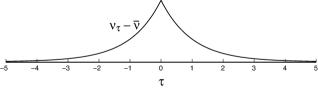
Figure 4: The time-symmetric, exponentially decaying stationary path associated with single-time $\delta$-function sources. This solution illustrates the embedding of the single-time equilibrium large-deviations theory within the richer time-dependent large-deviations theory of the stochastic process. In the forward direction, classical diffusion is responsible for the decay, and the response field $\eta\equiv 0$. In the reverse direction, $\eta$ back-propagates the constraint that a fluctuation of magnitude $\left({\nu}_{{\tau}_{C}}-\bar{\nu}\right)$ is observed at time ${\tau}_{C}$, and the dynamical-system representation generates the least-improbable trajectory of fluctuations that achieve that constraint.

The generating functional for the point source has the value already computed,

$$\Gamma\!\left[j\right] = {\Gamma}_{0}\!\left(0\right)-N\int_{0}^{\infty}d\tau\,{\partial}_{\tau}{\eta}^{\mbox{\scriptsize cl}}\,{\nu}^{\mbox{\scriptsize cl}}$$ (111)

$$= {\left.-N\log\cosh\frac{1}{2}\left({\eta}^{\mbox{\scriptsize cl}}-\beta\bar{\mu}\right)\right|}_{0}^{q},$$

again recovering Eq. (39). Note that although ${\nu}^{\mbox{\scriptsize cl}}\neq 0$ at all times, the integral receives contributions only from $\tau<{\tau}_{C}$ where $\eta\neq 0$.

The effective action is numerically just that given in Eq. (43), because it differs from the generating functional by subtraction of the point source $q{\nu}_{{\tau}_{C}}$ as before. However, as a Legendre transform on a space of histories, we now regard it as the functional

$$S^{\mbox{\scriptsize eff}}\!\left[n\right]=S^{\mbox{\scriptsize eff}}\!\left[N{\nu}^{\mbox{\scriptsize cl}}\right],$$ (112)

whose argument ${\nu}^{\mbox{\scriptsize cl}}$ is the whole exponential history given by Eq. (110) with ${\nu}_{{\tau}_{C}}$ fixed by Eq. (38). The entropy difference of Eq. (42) is now expressed not only as a probability of a fluctuation of given magnitude, but of the most-likely sequence of previous and subsequent configurations consistent with that observed fluctuation but with no other information given.

To understand the meaning of the stochastic effective action as a probability on histories, it is necessary to appreciate the non-local relation between histories and the structure of the moment-sampling currents $j$ which contain the minimal information to specify them. To extend the formulae for the effective action to more general histories, a variety of methods are known which produce both non-local and exact, or local but approximate, solutions.

IV.4.2 Continuous sources; linear-response approximation and analytic structure

We now return to the second-order expansion of Eq. (104) in fluctuations, from Sec. IV.2.6, but this time we complete the square directly rather than through a Hubbard-Stratonovich transformation. Following Onsager Onsager:RRIP1:31 ; Onsager:RRIP2:31 ; Onsager:Machlup:53 , we will expand about the equilibrium background where ${\nu}^{\mbox{\scriptsize cl}}\equiv\bar{\nu}$ and ${\eta}^{\mbox{\scriptsize cl}}\equiv 0$, and will simply write ${\eta}^{\prime}=\eta$. (The more general problem of expanding about non-classical backgrounds conditioned on sources could of course be considered as well.) The quadratic expansion of the action takes the simple form

$$S_{j} = -N\bar{\nu}\int_{0}^{\infty}d\tau j_{\tau}$$

$$\mbox{}+\int_{0}^{\infty}d\tau\left\{\left(\nu-\bar{\nu}\right)\left[\left(-{\partial}_{\tau}+1\right)\eta-j\right]-{\bar{\nu}}_{q}{\bar{\nu}}_{b}{\eta}^{2}\right\}.$$

The stationary-point equations are now linear-response equations,

$$\left(-{\partial}_{\tau}+1\right)\eta = j$$

$$\left({\partial}_{\tau}+1\right)\left(\nu-\bar{\nu}\right) = 2{\bar{\nu}}_{a}{\bar{\nu}}_{b}\eta.$$ (114)

$\eta$ is the response to $j$ through the advanced Green’s function:

$${\eta}_{\tau}=\int_{\tau}^{\infty}d{\tau}^{\prime}e^{\tau-{\tau}^{\prime}}j_{{\tau}^{\prime}},$$ (115)

while $\nu-\bar{\nu}$ responds through the symmetric Green’s function:

$${\nu}_{\tau}-\bar{\nu}={\bar{\nu}}_{a}{\bar{\nu}}_{b}\int_{0}^{\infty}d{\tau}^{\prime}e^{-\left|\tau-{\tau}^{\prime}\right|}j_{{\tau}^{\prime}}.$$ (116)

Eq. (116) reproduces the exact time dependence of Eq. (110) for a point source, and gives the linear small-$q$ approximation to the magnitude (38).

We now have a closed-form local expression for the generating functional in terms of the response field $\eta$ and the source $j$, because in these variables $\Gamma\!\left[j\right]$ is just $S_{j}$ evaluated on the stationary solution. From Eq. (114), this is

$$\Gamma\!\left[j\right]=-N\bar{\nu}\int_{0}^{\hat{T}}d\tau\,j_{\tau}-\frac{N}{2}\int_{0}^{\hat{T}}d\tau\left(2{\bar{\nu}}_{a}{\bar{\nu}}_{b}\right){\eta}^{2},$$ (117)

with $\eta$ given by Eq. (115). We recognize from Eq. (14), the quantity $N{\bar{\nu}}_{a}{\bar{\nu}}_{b}$ as the variance of the equilibrium distribution and hence the susceptibility to perturbations in chemical potential.

From the definition (233) and use of the equations of motion (114), the effective action is similarly expressed as a local functional,

$$S^{\mbox{\scriptsize eff}}\!\left[n\right] = \frac{N}{2}\int_{0}^{\infty}d\tau\frac{{\left[\left({\partial}_{\tau}+1\right)\left(\nu-\bar{\nu}\right)\right]}^{2}}{2{\bar{\nu}}_{a}{\bar{\nu}}_{b}}$$ (118)

$$= \frac{1}{2}\int_{0}^{\infty}d\tau\frac{{\left[\left({\partial}_{\tau}+1\right)\left(n-\bar{n}\right)\right]}^{2}}{2N{\bar{\nu}}_{a}{\bar{\nu}}_{b}}.$$

Eq. (118) is the expression first due to Onsager and Machlup Onsager:Machlup:53 . The first line, as usual, makes explicit the separation of large-deviations scaling in $N$ from the integral that is the rate function, which is a function only of fractional displacements $\nu-\bar{\nu}$.

IV.5 The relation to Onsager’s “minimum entropy production” property

Eq. (118) is a relation between an offset $n-\bar{n}$ and a transport current ${\partial}_{\tau}n$, which we might call $v$, a reaction velocity in appropriate units of time. Recalling Eq. (42) for the log-probability of single-time fluctuations, we may recognize the combination ${\left(n-\bar{n}\right)}^{2}/\left(2N{\bar{\nu}}_{a}{\bar{\nu}}_{b}\right)$ as none other than $S^{\mbox{\scriptsize eff}}\!\left(n\right)$, the entropy deficit from the equilibrium large-deviations principle. Immediately we would then recognize $\left(n-\bar{n}\right)/\left(N{\bar{\nu}}_{a}{\bar{\nu}}_{b}\right)$ as $\partial S^{\mbox{\scriptsize eff}}\!\left(n\right)/\partial n$, and $\left(n-\bar{n}\right)v/\left(N{\bar{\nu}}_{a}{\bar{\nu}}_{b}\right)$ as the rate of change in the equilibrium entropy of quasi-equilibrated subsystems. From these associations we could rewrite Eq. (118) in the form

$$S^{\mbox{\scriptsize eff}}\!\left[n\right] = \frac{1}{2}\int_{0}^{\infty}d\tau\left\{S^{\mbox{\scriptsize eff}}\!\left(n\right)+\frac{\partial S^{\mbox{\scriptsize eff}}\!\left(n\right)}{\partial n}v+\frac{1}{2}\frac{{\partial}^{2}S^{\mbox{\scriptsize eff}}\!\left(n\right)}{{\partial n}^{2}}v^{2}\right\},$$

in which the term ${\partial}^{2}S^{\mbox{\scriptsize eff}}\!\left(n\right)/{\partial n}^{2}$ gives the linear-response coefficients $1/\left(N{\bar{\nu}}_{a}{\bar{\nu}}_{b}\right)$.

If we chose to regard minimization of $S^{\mbox{\scriptsize eff}}\!\left[n\right]$ as an integral over time of two separate criteria – the first being the probability of a fluctuation to $n$ from $S^{\mbox{\scriptsize eff}}\!\left(n\right)$ and the second being a minimization over $v$ – the minimized function of $v$ given $n$ would be the “entropy production” relative to a bilinear form $v^{2}{\partial}^{2}S^{\mbox{\scriptsize eff}}\!\left(n\right)/{\partial n}^{2}$ parametrized by the near-equilibrium response coefficients. In two papers in 1931 Onsager:RRIP1:31 ; Onsager:RRIP2:31 , this was the result derived by Onsager as a consequence of microscopic reversibility and referred to as a “minimum entropy production” property. Onsager referred to the bilinear form of currents $v^{2}{\partial}^{2}S^{\mbox{\scriptsize eff}}\!\left(n\right)/{\partial n}^{2}$ as the “dissipation function”.

Note three things: 1) It is not the “entropy production” per se that is minimized, but only its value relative to the dissipation function, which from the form of the system entropy may be arbitrary; 2) there is no obvious reason to interpret the dissipation function as a “constraint” on the entropy production, and thus entropy production is not “minimized subject to constraints”, as an analogy to the way the entropy is maximized subject to constraints in equilibrium; and 3) the presence of the response coefficients in this form results from the near-equilibrium expansion, as is well-known.

We see, then, how we may speak precisely about the range of assumptions needed to make the “production” of the equilibrium entropy a quantity that is informative about dynamics. We have required the particular form of the local-equilibrium approximation that comes from a basins-and-barriers model, so that the dependence of the stochastic effective action $S^{\mbox{\scriptsize eff}}\!\left[n\right]$ on its instantaneous configuration variables reduces at leading order to the equilibrium quantity $S^{\mbox{\scriptsize eff}}\!\left(n\right)$. We have assumed small fluctuations in order to expand the linear velocity dependence in terms of $\partial S^{\mbox{\scriptsize eff}}\!\left(n\right)/\partial n$, and to approximate the linear response coefficients by their equilibrium values. Had all of these conditions not been satisfied, the expansion (LABEL:eq:S_eff_Onsager_Machlup_from_eq) need not have been valid. Yet, within the more general framework of the stochastic process, we could readily have derived the correct alternative form from the exact solution, which is derived as Eq. (233) in App. C. In the more general regime of non-linear response and large perturbations from the equilibrium distribution, the relation between a source $j\!\left(\tau\right)$ and the path $\nu\!\left(\tau\right)$ that it induces will generally be non-local in $\tau$.

IV.6 A second example: fixed dis-equilibria and an entropy rate for a large-deviation rate function

We now consider a second problem, aimed at relating dynamics to reference static distributions. Suppose that, rather than assuming free relaxation immediately after a fluctuation of magnitude (38), we ask for the probability of a history which remains at that value for a fixed time, and then freely decays. The difference of the effective action for this fixed-disequilibrium trajectory from that for a single-time fluctuation will give the entropy rate difference, between the stochastic process about the non-equilibrium steady state and the same process acting on the equilibrium distribution.

For this example, it is convenient to put the initial distribution at time $\tau\rightarrow-\infty$, to put the initial fluctuation at $\tau=0$ and hold it until ${\tau}_{C}$, and then to permit free decay after ${\tau}_{C}$ as before. From the constructions above, it is easy to define a source protocol that will produce this history. The source current takes the form

$$j_{\tau} = \Theta\!\left({\tau}_{C}-\tau\right)\Theta\!\left(\tau-0\right)\left[\sinh\frac{q}{2}+2\bar{\nu}\left(\cosh\frac{q}{2}-1\right)\right]$$ (120)

$$\mbox{}+\frac{q}{2}\left[\delta\!\left(\tau-{\tau}_{C}\right)+\delta\!\left(\tau-0\right)\right].$$

The stationary-point background evolves ${\eta}^{\mbox{\scriptsize cl}}$ unstably from its initial asymptotic value of zero at $\tau\rightarrow-\infty$ to value $q$ at $\tau=0-\epsilon$. The $\delta$-function in the source then lowers ${\eta}^{\mbox{\scriptsize cl}}$ to value $q/2$ at $\tau=0+\epsilon$, which solves the steady-state condition

$$\frac{\partial\hat{\mathcal{L}}}{\partial\nu}=j,$$ (121)

and holds it there until ${\tau}_{C}-\epsilon$, at which point the second $\delta$-function term takes ${\eta}^{\mbox{\scriptsize cl}}\rightarrow 0$ at $\tau={\tau}_{C}+\epsilon$. These results are easy to check from the exact equations of motion in action-angle coordinates, and the time-dependence of both $j_{\tau}$ and the associated ${\nu}^{\mbox{\scriptsize cl}}$ are shown in Fig. 5.

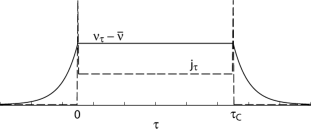
Figure 5: The source current (dashed) and resulting stationary solution (solid), for a source that raises $n_{\tau}$ to $n^{\left(q\right)}$ at $\tau=0$, holds it at this value until $\tau={\tau}_{C}$, and then releases it to free diffusive decay.

Because of the time-dependence of this source protocol $j$, neither $\hat{\mathcal{L}}$ nor ${\hat{\mathcal{L}}}_{j}$ vanishes. Indeed, because ${\partial}_{\tau}\eta=0$ except at the support of the $\delta$-functions of $j_{\tau}$, and because these two terms cancel in the action, the nonzero values of ${\hat{\mathcal{L}}}_{j}$ and $\hat{\mathcal{L}}$ determine $\Gamma$ and $S^{\mbox{\scriptsize eff}}$. We can check that these potentials evaluate to

$$\Gamma\!\left[j\right] = N\int d\tau\left(-{\partial}_{\tau}\eta\nu+{\hat{\mathcal{L}}}_{j}\right)$$ (122)

$$= N\left[\log\cosh\frac{\beta\bar{\mu}}{2}-\log\cosh\frac{1}{2}\left(q-\beta\bar{\mu}\right)\right]$$

$$\mbox{}-{\tau}_{C}\frac{N}{2}\left[\left(\cosh\frac{q}{2}-1\right)+2\bar{\nu}\sinh\frac{q}{2}\right]$$

and

$$S^{\mbox{\scriptsize eff}}\!\left[n\right] = N\int d\tau\left(-{\partial}_{\tau}\eta\nu+\hat{\mathcal{L}}\right)$$

$$= S^{\mbox{\scriptsize eff}}\!\left(n_{\tau=\left\{0,{\tau}_{C}\right\}}\right)+{\tau}_{C}\frac{N}{2}\frac{\cosh\frac{q}{2}-1}{\cosh\frac{\beta\bar{\mu}}{2}\cosh\frac{q-\beta\bar{\mu}}{2}}$$

$$= S^{\mbox{\scriptsize eff}}\!\left(n_{\tau=\left\{0,{\tau}_{C}\right\}}\right)+{\tau}_{C}N{\left(\sqrt{{\bar{\nu}}_{b}{\nu}_{a}}-\sqrt{{\bar{\nu}}_{a}{\nu}_{b}}\right)}^{2}.$$

${\hat{\mathcal{L}}}_{j}$ may be of either sign, while $\hat{\mathcal{L}}\geq 0$ always.

We may evaluate the $q\ll 1$ limit of Eq. (LABEL:eq:S_eff_holder_eval) for comparison to both the equilibrium effective action and the Onsager-Machlup linear approximation. Noting that in the linear-response regime $\left(\nu-\bar{\nu}\right)\rightarrow{\bar{\nu}}_{a}{\bar{\nu}}_{b}q$, the small-$q$ expansion becomes

$$S^{\mbox{\scriptsize eff}}\!\left[n\right]\rightarrow\frac{N{\bar{\nu}}_{a}{\bar{\nu}}_{b}q^{2}}{2}+{\tau}_{C}\frac{N{\bar{\nu}}_{a}{\bar{\nu}}_{b}q^{2}}{4}.$$ (124)

The probability of an initial fluctuation to non-equilibrium number occupancies is given by the equilibrium effective action, while the probability of persistence at that value is governed by a new term with the structure of an entropy rate Cover:EIT:91 . We will see in the Sec. V that this part of the effective action is a free-energy-rate difference, just as the equilibrium $S^{\mbox{\scriptsize eff}}\!\left(n\right)$ of Eq. (42) is a free-energy difference. The entropy-rate difference for persistent dis-equilibrium may be extracted as

$$\frac{\partial}{\partial{\tau}_{C}}S^{\mbox{\scriptsize eff}}\!\left[n\right] = N{\hat{\mathcal{L}}}_{\tau\in\left[0_{+},{\tau}_{C}\right]}$$ (125)

$$= \frac{N}{2}\frac{\cosh\frac{q}{2}-1}{\cosh\frac{\beta\bar{\mu}}{2}\cosh\frac{q-\beta\bar{\mu}}{2}}$$

$$= N{\left(\sqrt{{\bar{\nu}}_{b}{\nu}_{a}}-\sqrt{{\bar{\nu}}_{a}{\nu}_{b}}\right)}^{2}.$$

Eq. (125) is a new result. The combination of square-root dependence on quantities that equal the expected escape rates – ${\bar{\nu}}_{b}{\nu}_{a}$ and ${\bar{\nu}}_{a}{\nu}_{b}$ – and the squared difference of these in the exact entropy rate, extend to general multiparticle chemical reactions as shown in App. D.

To make contact with the Langevin treatment in Sec. IV.2.6, we check that in the persistent non-equilibrium domain where $\eta=q/2$, the fluctuation of the Langevin field in Eq. (97) is given by

$${\bar{\nu}}_{b}{\nu}_{a}^{\mbox{\scriptsize cl}}e^{{\eta}^{\mbox{\scriptsize cl}}}+{\bar{\nu}}_{a}{\nu}_{b}^{\mbox{\scriptsize cl}}e^{-{\eta}^{\mbox{\scriptsize cl}}}=2\sqrt{{\bar{\nu}}_{a}{\bar{\nu}}_{b}{\nu}_{a}^{\mbox{\scriptsize cl}}{\nu}_{b}^{\mbox{\scriptsize cl}}}.$$ (126)

The decay rate in the Langevin equation (96) evaluates to

$${\bar{\nu}}_{b}e^{{\eta}^{\mbox{\scriptsize cl}}}+{\bar{\nu}}_{a}e^{-{\eta}^{\mbox{\scriptsize cl}}}=\sqrt{\frac{{\bar{\nu}}_{a}{\bar{\nu}}_{b}}{{\nu}_{a}^{\mbox{\scriptsize cl}}{\nu}_{b}^{\mbox{\scriptsize cl}}}}.$$ (127)

Hence the single-time fluctuation expression (98) evaluates to

$$\left<{\left({\nu}^{\prime}_{\tau}\right)}^{2}\right>=\frac{{\nu}_{a}^{\mbox{\scriptsize cl}}{\nu}_{b}^{\mbox{\scriptsize cl}}}{N},$$ (128)

in agreement with the variance obtained from Eq. (98) for the distribution produced by the equilibrium generating function.

IV.6.1 The non-equilibrium entropy rate in relation to gradients of the equilibrium entropy

How does the entropy-rate difference defined from the dynamical stochastic effective action relate to changes in the equilibrium entropy of subsystems under free decay? We may recast Eq. (42) as

$$S^{\mbox{\scriptsize eff}}\!\left(n\right) = ND\!\left(\nu\parallel\bar{\nu}\right)$$ (129)

$$= \frac{N}{2}\left[\log\left(\frac{{\nu}_{b}{\nu}_{a}}{{\bar{\nu}}_{b}{\bar{\nu}}_{a}}\right)+q\left({\nu}_{b}-{\nu}_{a}\right)\right].$$

For the period of free decay after ${\tau}_{C}$, the change in equilibrium entropy with $n$ is

$$\frac{\partial}{\partial n}S^{\mbox{\scriptsize eff}}\!\left(n\right)=q.$$ (130)

The time-dependence of the equilibrium-form entropy follows from the time-dependence of $n$. Its gradient at the moment after the source perturbation is turned off is given by

$${\partial}_{\tau}n = -N\left(\nu-\bar{\nu}\right)$$ (131)

$$= -\frac{N}{2}\frac{\sinh\frac{q}{2}}{\cosh\frac{\beta\bar{\mu}}{2}\cosh\frac{q-\beta\bar{\mu}}{2}}.$$

Therefore, under free diffusion from a chemical-potential perturbation by $q$, the initial rate of subsystem entropy change is given by

$${\partial}_{\tau}S^{\mbox{\scriptsize eff}}\!\left(n\right) = \frac{\partial S^{\mbox{\scriptsize eff}}\!\left(n\right)}{\partial n}{\partial}_{\tau}n$$ (132)

$$= -\frac{N}{2}\frac{q\sinh\frac{q}{2}}{\cosh\frac{\beta\bar{\mu}}{2}\cosh\frac{q-\beta\bar{\mu}}{2}}.$$

At small $q$, $-{\partial}_{\tau}S^{\mbox{\scriptsize eff}}\!\left(n\right)\rightarrow 4\partial S^{\mbox{\scriptsize eff}}\!\left[n\right]/\partial{\tau}_{C}$ from Eq. (125). Thus the stochastic-process entropy rates, and the rate of change of equilibrium entropies, are not equal even in this limit; more generally they are distinct functions altogether. We can check from Eq. (125) that in the interval $\left[0,{\tau}_{C}\right]$, $\hat{\mathcal{L}}$ has the limits $\hat{\mathcal{L}}\rightarrow{\bar{\nu}}_{s}$ as $\tanh\left(q/2\right)\rightarrow 1$ and $\hat{\mathcal{L}}\rightarrow{\bar{\nu}}_{p}$ as $\tanh\left(q/2\right)\rightarrow-1$. Thus the entropy rate of the stochastic process is bounded by leaving-rates from the two respective states, while the corresponding rate of entropy change in Eq. (132) is unbounded.

We may summarize this section as follows: It should not be surprising that the stochastic effective action for histories includes entropy-rate terms that have no simple relation to rates of change in the equilibrium entropy of states. The former measures uncertainty about rates of transition, while the latter measures uncertainty about the occupation frequencies for states. It may be that, in some cases, dynamics is near enough to equilibrium that the state occupancy at successive moments of time places tight constraints on the possible entropy of transitions. However, this is not a general result, and it is not even implied by the local-equilibrium approximation of the form produced by the double-well potential. To say more about the origin of the rate term in the stochastic effective action (LABEL:eq:S_eff_holder_eval), however, requires a separation between system and environment terms that the continuous-time two-state model does not readily provide. For that separation we turn to the method of maximum caliber.

V Ensemble of histories II: resolved single-particle histories; path entropies and maximum caliber; structural decomposition into system and environment; connection to the stochastic-process entropy rate

The construction of equilibrium Gibbs free energies from the entropy, reviewed in App. B, begins with an explicit division between entropy terms for the system and its environment. The Freidlin-Wentzell construction of the preceding section does not naturally provide such a decomposition for paths, because the contribution of the “environment” comes from the form of the transition-rate terms $k_{\pm}$, which are embedded in the master equation. To separate these two contributions in the ensemble over histories, we require an explicit combinatorial formula for properties of paths, which is defined independently of the probabilities given to such paths by the transition rates set by the environment. The method of maximum caliber, as formulated in Ref’s Jaynes:caliber:80 ; Ghosh:caliber:06 ; Stock:caliber:08 ; Wu:caliber:09 , provides such a decomposition.

This section will introduce two changes of representation. One is the consideration of histories of an individual random walker, as explained in the introduction. The other, which will be more important to the ability to isolate system-environment interactions, is the replacement of the continuous-time stochastic process of the master equation (3), by a discrete-time two-state Markov process, shown in Fig. 6. The continuous-time and discrete-time models, in appropriate limits, represent the same stochastic process. However, the discrete-time model has the feature that, in every time interval of length $\Delta t$, some transition of the particle’s state must occur, even if it is a transition back to the same state.

Figure 6: Representation of the coarse-grained two-state system as a discrete finite-state model with forced transitions on every interval of length $\Delta t$.

It may come as a surprise when we find, below, that the entropy rate in the effective action (LABEL:eq:S_eff_holder_eval) draws its form entirely from the probabilities of no change. When we separate the large-deviations formula into contributions from the path entropy and the environmental probabilities, other terms associated with changes will also appear. However, these cancel exactly in the hydrodynamic limit represented by Eq. (LABEL:eq:S_eff_holder_eval). Thus we will see that, among the many terms that could have been used to probe the generating functional of the previous section, the particular coupling to the field $\nu$ that we studied was the form that produces the hydrodynamic limit. We return at the end of this section to what such a decomposition implies about the role of “energy dissipation” as an explanation for large-deviations probabilities of histories.

In the next two sections, we will solve for the path ensemble first in its stationary distribution, and then perturbed with sources. With appropriate choices for the transition parameters in the discrete model, the path ensemble will be constructed from the transfer matrix for the single-particle continuous-time model. With a particular choice of perturbing sources in the generating functional for this distribution, we will be able to show that the continuous-time Langevin equation gives the Gaussian approximation to the fluctuating single-particle trajectory.

V.1 Variational approach for a path ensemble in its stationary distribution, and connection to the continuous-time transfer matrix

The implementation of maximum-caliber in Ref’s. Stock:caliber:08 ; Wu:caliber:09 considers only steady trajectories displaced from the equilibrium. It does not consider time-dependent displacements, for which the Doi-Peliti formalism may provide easier constructions. However, the steady-state non-equilibrium problem does make contact directly with the constant-$j$ solutions of the preceding section.

For the stochastic process of Fig. 6 and a finite time interval $T$, consider four observables $M^{\alpha\beta}$, for $\alpha,\beta\in\left\{a,b\right\}$. These are the number of transitions from state $\beta$ to state $\alpha$ between $0$ and $T$. If we specify no more than these as constraints on a path entropy, they will tend toward uniform distribution on a long interval $T$, irrespective of the distribution we use to initialize paths.

The idea is to label each path with an index $j$, and to compute a path entropy

$$S^{\mbox{\scriptsize path}}\equiv-\sum_{j}p_{j}\log p_{j},$$ (133)

subject to some set of appropriate constraints on properties of the paths, such as its $M^{\alpha\beta}$ values, which will be denoted $M^{\alpha\beta}_{j}$. It will be convenient here to divide the path specification into the state in which the path starts, labeled with index $\sigma$, and the remainder of the path conditioned on that starting state, indexed $j\mid\sigma$. We could think, thus, of $j$ as a string denoting the ordered states through which the trajectory passed, and $j\mid\sigma$ as the string excluding its first letter. In this indexing $p_{j}=p_{j\mid\sigma}p_{\sigma}$.

It simplifies the treatment, without omitting any results that matter here, to exclude the distribution over over initial states from the variational problem, and to consider only variations of $p_{j\mid\sigma}$. For any path $j$, the numbers $M^{\alpha\beta}_{j}$ count the state-transitions from state $\beta$ to state $\alpha$ along that path. Denote by ${\bar{M}}^{\alpha\beta}$ the constraint values on maximum entropy for this path ensemble. Then the Lagrangian for the path-entropy maximization problem becomes

$${\mathcal{L}}^{\mbox{\scriptsize path}}\equiv-\sum_{\sigma}\sum_{j\mid\sigma}p_{j\mid\sigma}p_{\sigma}\log p_{j\mid\sigma}p_{\sigma}-\sum_{\alpha\beta}{\lambda}^{\alpha\beta}\left[\sum_{\sigma}\sum_{j\mid\sigma}p_{j\mid\sigma}p_{\sigma}M^{\alpha\beta}_{j}-{\bar{M}}^{\alpha\beta}\right]-\sum_{\sigma}{\eta}_{\sigma}\left[\sum_{j\mid\sigma}p_{j\mid\sigma}-1\right].$$ (134)

Lagrangians of the form (134) produce Gibbs (exponential) distributions as their maximizing distributions. Therefore, in terms of the Lagrange multipliers $\left\{{\lambda}^{\alpha\beta}\right\}$, the maximum-entropy probabilities have the form:

$$p_{j}=\frac{1}{Q}{\left({\gamma}^{aa}\right)}^{M^{aa}_{j}}{\left({\gamma}^{ab}\right)}^{M^{ab}_{j}}{\left({\gamma}^{ba}\right)}^{M^{ba}_{j}}{\left({\gamma}^{bb}\right)}^{M^{bb}_{j}}p_{\sigma}.$$ (135)

The entropy on this distribution was given the name caliber by Jaynes Jaynes:caliber:80 , to reflect the fact that it is a logarithmic measure of the width of a “tube” of microhistories which are typical within the distribution that produces macrohistories characterized by the $\left\{{\bar{M}}^{\alpha\beta}\right\}$.

Following Ref’s. Stock:caliber:08 ; Wu:caliber:09 (apart from a sign convention for the $\left\{{\lambda}^{\alpha\beta}\right\}$) we define

$${\gamma}^{\alpha\beta}\equiv e^{-{\lambda}^{\alpha\beta}},$$ (136)

and choose $p_{\sigma}$ to be the starting probability appropriate to whichever is the first state in history $j$. For this set of observables, the order in which transitions occur does not affect the weight function, though it does restrict the set of possible paths.

$Q$ is the partition function on histories, defined as the sum over $j$ of the other terms in Eq. (135). Because histories are in 1-1 correspondence with monomials that arise from the $M$th power of a $2\times 2$ matrix, the partition function is immediately expressed as the usual trace of a transfer matrix, just as we could have computed working directly from Eq. (44) above:

$$Q=\begin{array}[]{c}\left[\begin{array}[]{cc}1&1\end{array}\right]\\ \phantom{\left[\begin{array}[]{cc}1&1\end{array}\right]}\end{array}{\left(\left[\begin{array}[]{cc}{\gamma}^{aa}&{\gamma}^{ab}\\ {\gamma}^{ba}&{\gamma}^{bb}\end{array}\right]\right)}^{M}\left[\begin{array}[]{c}p_{a}\\ p_{b}\end{array}\right].$$ (137)

Now we may make some simplifying assumptions without loss of generality, to bring the expression (137) into direct correspondence with the transfer matrix of the continuous-time model. The matrix $\gamma$ does not actually have four independent values $\left\{{\gamma}^{\alpha\beta}\right\}$, because the original Lagrangian (134) did not have four independent constraints $\left\{{\bar{M}}^{\alpha\beta}\right\}$. The sum $\sum_{\alpha\beta}{\bar{M}}^{\alpha\beta}\equiv M$, because for each possible path also $\sum_{\alpha\beta}M^{\alpha\beta}_{j}\equiv M$. Moreover, for large $M$, it is not possible to set ${\bar{M}}^{ab}\neq{\bar{M}}^{ba}$ by more than $\pm 1$, so effectively these must be chosen equal. Therefore two normalizations of the $\left\{{\gamma}^{\alpha\beta}\right\}$ may be chosen arbitrarily. These may be chosen so that ${\gamma}^{aa}+{\gamma}^{ba}=1$, ${\gamma}^{ab}+{\gamma}^{bb}=1$, effectively choosing unit normalization for the partition function $Q$. The matrix $\left[{\gamma}^{\alpha\beta}\right]$ is then called a stochastic matrix.

Next, in keeping with the omission of the initial state from the variational problem, suppose $p_{\sigma}$ is chosen to be the stationary distribution of largest eigenvalue preserved by whatever values of ${\gamma}^{\alpha\beta}$ solve the variational problem. Then it follows immediately – by collapse of the matrix $\left[{\gamma}^{\alpha\beta}\right]$ with $\left[\begin{array}[]{cc}1&1\end{array}\right]$ on the left, and with ${\left[\begin{array}[]{cc}p_{a}&p_{b}\end{array}\right]}^{T}$ on the right – that

$$\frac{\partial\log Q}{\partial\log{\gamma}^{\alpha\beta}}=\left<M^{\alpha\beta}_{j}\right>=M{\gamma}^{\alpha\beta}p_{\beta}.$$ (138)

We solve for the $\left\{{\gamma}^{\alpha\beta}\right\}$ by setting Eq. (138) equal to ${\bar{M}}^{\alpha\beta}$. It follows from our choice to normalize $\left[{\gamma}^{\alpha\beta}\right]$ to be a stochastic matrix that

$$\sum_{\alpha}\frac{{\bar{M}}^{\alpha\beta}}{M}=p_{\beta}.$$ (139)

The relation of the $\left\{{\gamma}^{\alpha\beta}\right\}$ to the $\left\{p_{\beta}\right\}$ may now be made explicit. The assumption behind the use of a discrete stochastic-process model is that $\Delta t$ is a scaling variable that may be changed in the discrete model while leaving important physical observables unchanged, though rescaling $\Delta t$ may introducing overall renormalization constants associated with the discretization. In general the $\left\{{\gamma}^{\alpha\beta}\right\}$ will then depend on the $\Delta t$ but the stationary distribution of the stochastic process should not. Denote the stationary distribution that is self-consistent with the $\left\{{\gamma}^{\alpha\beta}\right\}$ appropriate to the given $\left\{{\bar{M}}^{\alpha\beta}\right\}$ by $\left[{\pi}_{\beta}\right]$. Then the most general stochastic matrix $\left[{\gamma}^{\alpha\beta}\right]$ with $\left[{\pi}_{\beta}\right]$ as the dominant eigenvector is

$$\left[\begin{array}[]{cc}{\gamma}^{aa}&{\gamma}^{ab}\\ {\gamma}^{ba}&{\gamma}^{bb}\end{array}\right]=\left\{\left[\begin{array}[]{cc}1&\\ &1\end{array}\right]+\left[\begin{array}[]{cc}-{\pi}_{b}&{\pi}_{a}\\ {\pi}_{b}&-{\pi}_{a}\end{array}\right]\left(1-r^{-R}\right)\right\}.$$ (140)

The constant $R$ sets the frequency of transition events $M^{ab}=M^{ba}$. To model ensure that the discrete stochastic process has the same continuum limit as the continuous-time model of the previous sections, we require that for sufficiently short $\Delta t$, $R$ must converge to

$$R=\left(k_{+}+k_{-}\right)\Delta t.$$ (141)

The form (140) is chosen so that under refinement or coarsening of the time increment, the definition (141) remains consistent.

The interpretation of $k_{\pm}$ as rate constants is completed if we set their ratio from the fractions of time intervals in which the system starts, respectively, in states $a$ or $b$:

$${\pi}_{a} = \frac{k_{-}}{k_{+}+k_{-}}$$

$${\pi}_{b} = \frac{k_{+}}{k_{+}+k_{-}},$$ (142)

corresponding to Eq. (10). Values of $k_{\pm}$ are then chosen to satisfy the constraints (139). With these choices the matrix $\left[{\gamma}^{\alpha\beta}\right]$ becomes precisely the transfer matrix for the continuous-time one-particle problem.

Note that the relation between the rate constants, equilibrium frequencies, and transition numbers may be written

$$\frac{{\bar{M}}^{ba}}{T}=\frac{{\bar{M}}^{ab}}{T}=\sqrt{{\pi}_{a}k_{+}}\sqrt{{\pi}_{b}k_{-}}.$$ (143)

This form – a variant expression for either ${\pi}_{a}k_{+}$ or ${\pi}_{b}k_{-}$ – which characterizes the equilibrium distribution, will arise again when we use the generating function to probe steady non-equilibrium states.

From the variational property (138) and the original Lagrangian formulation of the problem, we recognize that $\log Q$ will be the negative of a Gibbs free energy. From the fact that $\log Q\equiv 0$ when the $\left\{{\gamma}^{\alpha\beta}\right\}$ are evaluated at the above conditions, we know that the free energy may be offset by a constant at the entropy-maximizing, equilibrium distribution. We may derive the exact relation by calculating the entropy of paths (the caliber) on the solution (135),

$$S^{\mbox{\scriptsize path}}\!\left[\left\{{\bar{M}}^{\alpha\beta}\right\}\right]=-\sum_{\alpha}{\pi}_{\alpha}\log{\pi}_{\alpha}+\sum_{\alpha\beta}\left<M^{\alpha\beta}\right>{\lambda}^{\alpha\beta}$$

$$= -\sum_{\alpha}{\pi}_{\alpha}\log{\pi}_{\alpha}-\sum_{\alpha\beta}{\bar{M}}^{\alpha\beta}\log\frac{{\bar{M}}^{\alpha\beta}}{M{\pi}_{\beta}}$$

$$= -\sum_{\alpha}{\pi}_{\alpha}\log{\pi}_{\alpha}-M\sum_{\beta}{\pi}_{\beta}\sum_{\alpha}{\gamma}^{\alpha\beta}\log{\gamma}^{\alpha\beta}.$$

(144)

The first line of Eq. (144) is simply the evaluation of the definition (133), recalling that $\log Q=0$ in the normalization of $p_{j}$. The second line is the proper extensive-form dependence of the entropy on the constraint variables which are its macroscopic arguments. The third line, interpreting the $\left\{{\gamma}^{\alpha\beta}\right\}$ as transition probabilities in the state diagram of Fig. (6), expresses the path entropy as a sum of the entropy of the initial distribution, with the time-integral of the entropy rate of the stochastic process in that distribution Cover:EIT:91 . This expression is the first in the paper, in which the entropy rate is given its familiar form from the stochastic process of a finite-state system.

The combinatorial interpretation of the second line in Eq. (144) is immediate. Using $S^{0}\!\left(\left\{{\pi}^{\alpha}\right\}\right)$ to denote the single-time entropy of the initial distribution, we may express

$$S^{\mbox{\scriptsize path}}\!\left[\left\{{\bar{M}}^{\alpha\beta}\right\}\right]=S^{0}\!\left(\left\{{\pi}^{\alpha}\right\}\right)+\log\left(\begin{array}[]{c}M{\pi}_{a}\\ {\bar{M}}^{ba}\end{array}\right)+\log\left(\begin{array}[]{c}M{\pi}_{b}\\ {\bar{M}}^{ab}\end{array}\right).$$ (145)

The combinatorial entropy is the Stirling approximation for the logs of the two independent binomial factors for distributing ${\bar{M}}^{ba}$ transitions $a\rightarrow b$ among $M{\pi}_{a}={\bar{M}}^{aa}+{\bar{M}}^{ba}$ total exits from state $a$, and similarly for distributing ${\bar{M}}^{ab}$ exits $b\rightarrow a$ among $M{\pi}_{b}$ total exits from $b$. Note that the entropy rate term in Eq. (144) will diverge logarithmically in $\Delta t$ if a finite number of transitions ${\bar{M}}^{ba}={\bar{M}}^{ab}$ is fixed in a growing number of opportunities $M$.

Finally, from the explicit expression for the entropy either in terms of $\left\{{\bar{M}}^{\alpha\beta}\right\}$ or the associated Lagrange multipliers $\left\{{\lambda}^{\alpha\beta}=-\log{\gamma}^{\alpha\beta}\right\}$, we may identify the relation between the partition function $Q$ and a free energy that leads to the relations (138)

$$-\log Q=\sum_{\alpha\beta}{\lambda}^{\alpha\beta}{\bar{M}}^{\alpha\beta}_{\lambda}-S^{\mbox{\scriptsize path}}\!\left[\left\{{\bar{M}}^{\alpha\beta}_{\lambda}\right\}\right]+S^{0}\!\left(\left\{{\pi}^{\alpha}\right\}\right).$$ (146)

Here each ${\bar{M}}^{\alpha\beta}_{\lambda}$ denotes the $\alpha\beta$-component of the set of $\bar{M}$ jointly satisfying

$$\frac{\partial S^{\mbox{\scriptsize path}}\!\left[\left\{{\bar{M}}^{\alpha\beta}\right\}\right]}{\partial{\bar{M}}^{\alpha\beta}}={\lambda}^{\alpha\beta}.$$ (147)

From the developments of the single-time equilibrium, we may anticipate that the effective action for other configurations $\left\{{\bar{M}}^{\alpha\beta}\right\}$ than the most-probable ones will have the same form as Eq. (146), with $\left\{{\lambda}^{\alpha\beta}\right\}$ fixed and $\left\{{\bar{M}}^{\alpha\beta}\right\}$ permitted to vary independently of them. We will return to that and to its physical and combinatorial evaluation in a moment, but first we do the construction methodically through a generating function for the path-probability distribution.

V.2 Generating function for steady non-equilibrium states, and connection to the continuous-time Langevin equation

A generating function for the discrete-time path ensemble may be constructed as it was in the Doi-Peliti method. Because we will consider only steady non-equilibrium distributions, we may do this in a direct and simple way, as a modification of the underlying transfer matrix by shifts in the chemical potential. There are many perturbations that could be chosen for the discrete-time model, but only the one equivalent to the coupling to the number field in Sec. IV.3 produces the same hydrodynamic limit as $\Delta t\rightarrow 0$.

Because the discrete model has four parameters $\left\{{\gamma}^{\alpha\beta}\right\}$ for transition rates, we introduce four complex variables

$$z^{\alpha\beta}\equiv e^{{\zeta}^{\alpha\beta}}$$ (148)

as arguments of the moment-generating function. Suppose that, like the ${\lambda}^{\alpha\beta}$, all ${\zeta}^{\alpha\beta}$ scale $\sim\left(k_{+}+k_{-}\right)\Delta t\ll 1$. The terms ${\zeta}^{ba}$ and ${\zeta}^{ab}$ modify the transition currents, while terms ${\zeta}^{aa}$ and ${\zeta}^{bb}$ modify the persistence probabilities. The counterpart to the current $j$ of Sec. IV.3, which effectively modifies the chemical potentials of the states, is the combination ${\zeta}^{aa}-{\zeta}^{bb}$. Therefore, to compare the path entropy to this perturbation in the Doi-Peliti formulation, we set ${\zeta}^{ba}={\zeta}^{ab}\equiv 0$, and consider only the remaining two perturbations.

For constant sources $z^{aa}$ and $z^{bb}$, the path-generating function for non-equilibrium, asymptotically-steady transition numbers may simply be written in terms of a transfer matrix that has the same modification in every timestep, as

$${\psi}^{\mbox{\scriptsize path}}\!\left(z^{aa},z^{bb}\right)\equiv e^{-{\Gamma}^{\mbox{\scriptsize path}}\left({\zeta}^{aa},{\zeta}^{bb}\right)}$$ (157)

$$= \sum_{\sigma}\sum_{j\mid\sigma}{\left(z^{aa}\right)}^{M^{aa}_{j}}{\left(z^{bb}\right)}^{M^{bb}_{j}}p_{j\mid\sigma}{\pi}_{\sigma}$$

$$= \frac{1}{Q}\begin{array}[]{c}\left[\begin{array}[]{cc}1&1\end{array}\right]\\ \phantom{\left[\begin{array}[]{cc}1&1\end{array}\right]}\end{array}{\left(\left[\begin{array}[]{cc}{\gamma}^{aa}z^{aa}&{\gamma}^{ab}\\ {\gamma}^{ba}&{\gamma}^{bb}z^{bb}\end{array}\right]\right)}^{M}\left[\begin{array}[]{c}{\pi}_{a}\\ {\pi}_{b}\end{array}\right].$$

The starting probabilities $\left\{{\pi}_{\sigma}\right\}$ in Eq. (157) will no longer be those preserved by the transfer matrix at nonzero $\left\{{\zeta}^{\alpha\beta}\right\}$, so the function ${\Gamma}^{\mbox{\scriptsize path}}\!\left({\zeta}^{aa},{\zeta}^{bb}\right)$ will generally differ from the form (146) given for $-\log Q$. The difference will be associated with transient decay from $\left\{{\pi}_{\sigma}\right\}$ to the perturbed stationary state, and will scale as ${\left(T\right)}^{0}$ at large $T$. If we denote this constant as ${\Lambda}^{0}$, the asymptotic expression for the generating function becomes

$${\Gamma}^{\mbox{\scriptsize path}}\!\left({\zeta}^{aa},{\zeta}^{bb}\right) = \sum_{\alpha\beta}{\left(\lambda+\zeta\right)}^{\alpha\beta}{\bar{M}}^{\alpha\beta}_{\left(\lambda+\zeta\right)}-S^{\mbox{\scriptsize path}}\!\left[\left\{{\bar{M}}^{\alpha\beta}_{\left(\lambda+\zeta\right)}\right\}\right]$$ (158)

$$\mbox{}+{\Lambda}^{0}+\log Q.$$

The asymptotic stationary values ${\bar{p}}^{a}$, ${\bar{p}}^{b}$ may be computed as functions of $\lambda+\zeta$ as before, and the functional relation may then be inverted to assign values to the ${\zeta}^{\alpha\beta}$. It is possible to check that only the combination ${\zeta}^{aa}-{\zeta}^{bb}$ appears in any of the transition-number expressions, so we could originally have set $z^{aa}=1/z^{bb}$ as a single argument to ${\psi}^{\mbox{\scriptsize path}}$. This construction exactly follows the construction of the two-argument and the one-argument moment-generating functions in Sec. III.2.

An important secondary relation that is not merely a definition but results from the choice ${\zeta}^{ba}={\zeta}^{ab}\equiv 0$, is that the off-equilibrium transition rates satisfy

$$\frac{{\bar{M}}^{ba}_{\left(\lambda+\zeta\right)}}{T}=\frac{{\bar{M}}^{ba}_{\left(\lambda+\zeta\right)}}{T}=\sqrt{{\bar{p}}_{a}k_{+}}\sqrt{{\bar{p}}_{b}k_{-}}.$$ (159)

Eq. (159) is the counterpart to Eq. (143) for the equilibrium distribution. This property will be responsible for the cancellation of terms between the path entropy and external weight factors which could diverge as $\Delta t\rightarrow 0$, and recovery of the hydrodynamic limit.

The transition rates (159) equal the rate at which the Langevin field correlation function (97) injects noise into the number-field correlation function (98). Thus we confirm that, for this simple example of non-interacting particles, the Langevin equation (96) describes the fluctuating trajectories of single-particle states. The Langevin description is indirect, as ${\nu}^{\prime}$ is formally the expectation value of a Poisson distribution, and not a discrete single-particle trajectory. Following the injection of noise by the correlation function, it is then the classical relaxation time of these fluctuations, given by Eq. (127), that causes the single-time fluctuations (98) to agree with those in the equilibrium generating-function distribution from Eq. (32). We thus establish the mutual consistency of all of the approaches used.

V.3 The effective action from caliber and its interpretation

From here we compute the effective action by Legendre transform, just as in Sec. III for the single-time equilibrium distribution. The result is

$$S^{\mbox{\scriptsize eff}}\!\left[\left\{{\bar{M}}^{\alpha\beta}\right\}\right]={\Gamma}^{\mbox{\scriptsize path}}\!\left({\zeta}^{aa}_{\bar{M}},{\zeta}^{bb}_{\bar{M}}\right)-{\zeta}^{aa}_{\bar{M}}{\bar{M}}^{aa}-{\zeta}^{bb}_{\bar{M}}{\bar{M}}^{bb}$$ (166)

$$= \sum_{\alpha\beta}{\lambda}^{\alpha\beta}{\bar{M}}^{\alpha\beta}-S^{\mbox{\scriptsize path}}\!\left[\left\{{\bar{M}}^{\alpha\beta}\right\}\right]+{\Lambda}^{0}+\log Q$$

$$= \sum_{\alpha}{\lambda}^{\alpha a}{\bar{M}}^{\alpha a}-\log\left(\begin{array}[]{c}M{\bar{p}}_{a}\\ {\bar{M}}^{ba}\end{array}\right)$$

$$\mbox{}+\sum_{\alpha}{\lambda}^{\alpha b}{\bar{M}}^{\alpha b}-\log\left(\begin{array}[]{c}M{\bar{p}}_{b}\\ {\bar{M}}^{ab}\end{array}\right)$$

$$\mbox{}+{\Lambda}^{0}+\log Q.$$

In the last expression we recall the decomposition (145) of the stationary-state path entropy into the logarithms of two independent binomials. For the equilibrium transition rates ${\Lambda}^{0}\rightarrow S^{0}\!\left(\left\{{\pi}^{\alpha}\right\}\right)$ and the expression vanishes as required. Recalling that $S^{0}\!\left(\left\{{\pi}^{\alpha}\right\}\right)+\log Q$ in Eq. (146) is simply the maximizer of the terms written explicitly in Eq. (166), we recover exactly the difference of Gibbs free energies which was the stochastic effective action in Eq. (42).

It now remains only to check that the expression (166) recovers the non-divergent entropy rate computed from the master equation, and to assign physical meanings to the terms that appear.

Consider the limit in which $M^{ba}=M^{ab}$ remains finite as $\Delta t\rightarrow 0$ and $M\rightarrow\infty$, and suppose all $k_{\pm}\Delta t\ll 1$. The external source term that appears in the effective action (166) evaluates to

$$\frac{\sum_{\alpha\beta}{\lambda}^{\alpha\beta}{\bar{M}}^{\alpha\beta}}{T} = -\frac{M{\bar{p}}^{a}-M^{ba}}{M\Delta t}\log\left(1-k_{+}\Delta t\right)-\frac{M{\bar{p}}^{b}-M^{ab}}{M\Delta t}\log\left(1-k_{-}\Delta t\right)-\frac{M^{ba}}{T}\log\left(k_{+}\Delta t\right)+\frac{M^{ab}}{T}\log\left(k_{-}\Delta t\right)$$ (167)

$$= {\bar{p}}_{a}k_{+}+{\bar{p}}_{b}k_{-}-\sqrt{{\bar{p}}_{a}k_{+}{\bar{p}}_{b}k_{-}}\log\left(k_{+}k_{-}{\Delta t}^{2}\right).$$

The first two terms in the second line, although proportional to the expected escape rates from the two wells with occupancies ${\bar{p}}_{a}$, ${\bar{p}}_{b}$, actually come from the accumulation of time intervals in which the particle does not escape and whose likelihoods differ from unity only by $k_{\pm}\Delta t$. This accumulation of terms would not be affected even if we made finite changes in $M^{ba}$ or $M^{ab}$, as long as total $M$ was sufficiently large. The other term, containing the logarithm, comes from the unlikely events in which sufficient energy accumulates in a fluctuation to induce a barrier crossing. It is simply the product of Boltzmann factors on a set of independent intervals of length $\Delta t$, whose total number is $M^{ba}+M^{ab}$.

The terms in the purely combinatorial path entropy evaluate to

$$\frac{S^{\mbox{\scriptsize path}}\!\left[\left\{{\bar{M}}^{\alpha\beta}\right\}\right]}{M} = -\frac{M{\bar{p}}^{a}-M^{ba}}{M}\log\left(1-\frac{M^{ba}}{M{\bar{p}}^{a}}\right)-\frac{M{\bar{p}}^{b}-M^{ab}}{M}\log\left(1-\frac{M^{ab}}{M{\bar{p}}^{b}}\right)-\frac{M^{ba}}{M}\log\frac{M^{ba}}{M{\bar{p}}^{a}}-\frac{M^{ab}}{M}\log\frac{M^{ab}}{M{\bar{p}}^{b}}$$ (168)

$$\approx \frac{M^{ba}}{M}\left[2-\log\left(\frac{M^{ba}M^{ab}}{M^{2}{\bar{p}}_{a}{\bar{p}}_{b}}\right)\right]$$

$$= \Delta t\sqrt{{\bar{p}}_{a}k_{+}{\bar{p}}_{b}k_{-}}\left[2-\log\left(k_{+}k_{-}{\Delta t}^{2}\right)\right].$$

We have placed the terms in the same order as those in the external linear function (167), and the term with the logarithm – again arising from the events where the state changes – is in fact identical in the entropy and in Eq. (167). The two log terms exactly cancel in the subtraction that defines the effective action (166), leaving a finite remainder, which we will see is the hydrodynamic entropy rate.

It is the first two, non-divergent term, which differ between the path entropy and the external probabilities. The total numbers $M^{ba}$ and $M^{ab}$ are frequencies entering the binomial factors in the path entropy, and both terms contribute identical factors proportional to $M^{ba}=M^{ab}$. The difference of Eq. (167) and Eq. (168) gives the non-divergent effective action by Eq. (166), which goes at large $T$ (ignoring the contribution of terms $\sim{\left(T\right)}^{0}$) to

$$\frac{S^{\mbox{\scriptsize eff}}\!\left[\left\{{\bar{M}}^{\alpha\beta}\right\}\right]}{T} \rightarrow {\bar{p}}_{a}k_{+}+{\bar{p}}_{b}k_{-}-2\sqrt{{\bar{p}}_{a}k_{+}{\bar{p}}_{b}k_{-}}$$ (169)

$$= {\left(\sqrt{{\bar{p}}_{a}k_{+}}-\sqrt{{\bar{p}}_{b}k_{-}}\right)}^{2}.$$

Eq. (169) recovers precisely the 1-particle coefficient of $t_{C}$ in Eq. (LABEL:eq:S_eff_holder_eval), when converted to descaled time ${\tau}_{C}$ by the factor $k_{+}+k_{-}$.

Thus we again find that $T$ is the scaling variable in the large-deviations principle associated with independent path fluctuations for a single particle. This scaling applies only to the extended-time partition function. It acts independently of the scaling with $N$, which is the same in the extended-time and single-time levels of thermodynamic description.

V.4 Discretization divergences and the natural scale

As was explained in Sec. II.5, the discrete time interval $\Delta t$ may be taken only down to a certain scale, before the approximation by a discrete two-state theory becomes inappropriate. The lower limit to $\Delta t$ from the continuum double-well model will come from the diffusive relaxation time, for a trajectory starting at the saddle point and ending in whichever well is most-quickly reached. On timescales shorter than this, it becomes invalid to characterize escapes as elementary events counted by $M^{ba}_{j}$ or $M^{ab}_{j}$.

We expect that when the discretization scale is set to this value – termed the natural scale of the problem following Ref. Polchinski:RGEL:84 – the arguments of the logarithms in Equations (167,168) become

$$\Delta tk_{\pm}\approx 2\pi e^{-\beta\left({\mu}_{\ddagger}-{\mu}_{a/b}^{1}\right)}.$$ (170)

The exponential waiting times in $k_{\pm}$ are not affected, but the factor $\Delta t$ cancels the dimensional prefactors in $k_{\pm}$, which have dimensions $1/\mbox{time}$, and have a characteristic scale set by the diffusive relaxation rate.

If we plug the approximation (170) into the formula (167) for the environment terms in the path-space Gibbs free energy, this term evaluates approximately to

$$\frac{\sum_{\alpha\beta}{\lambda}^{\alpha\beta}{\bar{M}}^{\alpha\beta}}{T} \approx {\bar{p}}_{a}k_{+}+{\bar{p}}_{b}k_{-}$$

$$\mbox{}+\frac{{\bar{M}}^{ba}}{T}\beta\left({\mu}_{\ddagger}-{\mu}_{a}^{1}\right)+\frac{{\bar{M}}^{ab}}{T}\left({\mu}_{\ddagger}-{\mu}_{b}^{1}\right).$$

We have thus arrived at a mathematical expression of the graphical heuristic for thinking about dynamical ensembles given in Fig. 3 of Sec. II.3. The attracting fixed points of the underlying free-energy landscape carry charge-valued, extensive state variables such as the occupation frequencies ${\bar{p}}_{a}$, ${\bar{p}}_{b}$ for states. They are related under Legendre transform to dual, intensive entropy gradients from the environment – here $k_{+}$ and $k_{-}$ respectively – which determine the probabilities for each state. The extensive, current-valued state variables – here the numbers ${\bar{M}}^{ba}$ and ${\bar{M}}^{ab}$ of transition events – live on the saddle points of the landscape. Under Legendre transform, they should be coupled to the dual chemical potentials that determine the probability of transitions: here ${\mu}_{\ddagger}-{\mu}_{a}^{1}$ and ${\mu}_{\ddagger}-{\mu}_{b}^{1}$. The asymmetry between states and transitions arises because chemical potentials appear exponentially in the leaving rates $k_{\pm}$, and only linearly in the transition-state terms involving ${\mu}_{\ddagger}$.

V.5 Connection to energy dissipation

The path-space Gibbs free energy (166) has separated events into categories, which we can associate with different kinds of energy transfers. The events in which the particle exchanges wells could correctly be associated with either absorption of energy from the bath, or dissipation to it, depending on the sign of the free-energy difference in the starting and ending well. However, these terms entirely cancel between the path entropy and the environment-mediated probability, and do not contribute to the entropy rate expression in Eq. (LABEL:eq:S_eff_holder_eval) in the hydrodynamic limit. This cancelling term may be ascribed to “entropy production” in the path ensemble which is exported to the environment, but it does not appear in the large-deviations formula. Moreover, we are lucky that we do not need it to compute path-probabilities, because it appears to depend on the model resolution $\Delta t$, which is not physically meaningful.

The terms that survive in the entropy rate, and contribute to its distinctive form (125), come from all the moments when thermal fluctuations do not lead to escapes. For all these, energy is neither absorbed nor dissipated. In summary, we acknowledge that there are cases Jarzynski:fluctuations:08 in which a collection of non-equilibrium transitions is constrained by consistency with the equilibrium distribution that is their starting or ending point. Since the equilibrium distribution is dictated by energy, these constrained transformations must also have characterizations in terms of energy. However, for a large collection of non-equilibrium fluctuation theorems, energy alone is not serving as the primary constraint on kinetics, and we must look for the explanation of path probabilities in terms of other parameters of the stochastic process.

VI Discussion and conclusions

VI.1 Why generating functions for large-deviations formulae?

We remarked in Sec. IV.1 that generating functions provide a more natural representation for large-deviation formulae, and better approximation methods, than the discrete probability distribution, because generating functions expand in moments of collective many-particle motion, rather than in single-particle hops. We have also seen, comparing Eq. (19) to Eq. (42), that the cumulant-generating function extracts the leading exponential term in from the probability distribution, bypassing sub-leading terms from normalization. But how does it perform this separation? We may understand that the isolation of leading exponentials is in fact a direct reflection of the way the generating function expands in moments.

In elementary statistical mechanics Kittel:TP:80 , we argue that the microcanonical and canonical ensembles produce the same entropy, because the probability of the most-likely element in a sharply peaked distribution is equal at leading exponential order to the weight of all typical elements in that distribution. The two probabilities differ only by the width of the distribution, which is sub-leading as we saw in Eq. (22).

The moment-generating function may be understood as extracting, not only the probability to observe a single sample-fluctuation from the equilibrium distribution, but in fact the projection of the original distribution onto the entire sub-distribution within which that sample fluctuation is typical. This is the shifted binomial distribution appearing in Eq. (29). The constant of proportionality between the two distributions, whose logarithm is the cumulant-generating function, is then precisely the leading exponential difference of probabilities, because normalization terms in the original distribution and the projected distribution have canceled.

VI.2 Operator algebras in the Doi formalism; two-field methods in general, and the difference between classical and quantum systems

The Doi Doi:SecQuant:76 ; Doi:RDQFT:76 construction of time-dependent ensembles uses a further property of generating functions which can lead to confusion on first exposure, but which is important to understand in order to assign the correct meaning to the operators and states used in the construction.

Any probability distribution may be written as a sum of modes, and the generating function associated with that probability distribution may likewise be written as a sum of polynomials. Therefore, generating functions satisfy a property of superposition, similar in many respects to the superposition satisfied by states in quantum mechanics. Time evolution acts on superpositions, either of quantum states, or of the modes of a generating function, independently. Much of the time-dependence in either quantum mechanics or stochastic processes can therefore be understood from the sequencing of the time-evolution operators, without reference to the particular function-spaces in which they act. Doi’s contribution was to distill the dependence in the order of time-evolution operators into an operator algebra, which has the same form as the algebra of the simple harmonic oscillators of quantum mechanics or quantum field theory.

For this reason, Doi-Peliti methods are sometimes Mattis:RDQFT:98 termed “Quantum Field Theory” methods for stochastic processes. However, the operator algebra itself carries no implication of a physical property of quantum-superposition of distinct eigenstates of observables, and derives only from the linearity of time evolution. The physical commitment to the classical or quantum nature of a system comes from specifying the space of functions representing states and their observable properties, and on the inner product in that space. For further discussion of the many similarities implied, solely by superposition and causality, between classical and quantum systems, see Ref. Kamenev:DP:01 . It is under the correspondence of operator algebras that the stochastic effective action and the quantum effective action are equivalent objects.

The use of time-dependent sources to probe complex histories with the stochastic effective action does not seem common in reaction-diffusion applications of Doi-Peliti theory. We hope that such methods can come to be used to ask a wider range of structurally explicit questions about non-equilibrium paths.

As the simplest non-trivial examples, this paper has demonstrated new entropy-rate formulae for steady non-equilibrium paths, both for independent-particle random walks, and for stoichiometrically non-trivial chemical reactions. An area for future work is to extend such formulae to study the large-deviations behavior of random walks on graphs or the fluctuations of realistic chemical-reaction networks.

VI.3 The information conditions that embed single-time ensembles within ensembles of histories

The equilibrium (canonical) thermodynamic ensemble was recovered in Sec. IV.3 as the projection of the larger ensemble over histories onto a single time slice, in a region where the histories had settled into their stationary distribution over both states and transitions. “Fluctuations” in the equilibrium ensemble have no dynamical connotation, and are simply sample values. Histories have both dynamical correlation – a property of a path itself – and stochastic fluctuation that represents sampling from the ensemble over paths.

Fluctuation values in the equilibrium ensemble, when embedded within the larger ensemble of histories, have the interpretation of instantaneous conditions on histories accompanied by no other information. These information conditions imply distributions over histories conditioned on the single-time fluctuation, which appears as an independent variable. Freidlin-Wentzell theory reproduces the probabilities for such single-time fluctuations from the integrals, over the most-probable histories, of conditional probabilities for each successive increment of change.

The equilibrium distribution is not the only ensemble that can be recovered from an ensemble of histories by projection onto single instants. Projections onto slices where paths have not settled into their stationary distribution result in non-equilibrium entropies at single times. These entropies require both charge and current state variables as arguments Smith:dual:05 ; Smith:DP:08 , and they can be written in terms of the Wigner distribution, considered in Ref. Smith:evo_games: . We may say, then that there is a hierarchy of ensembles, from the most-complete ensemble over histories, to single-time non-equilibrium ensembles, which lose the time-correlation of histories but preserve current-valued state variables, finally reaching the equilibrium ensemble, which projects onto only the charge-valued state variables. By connecting state variables to fixed points of free-energy landscapes in Fig. 3 , and to Legendre duality in Eq. (LABEL:eq:ext_rates_path_nat_scale), we have attempted to provide several perspectives to understand this duality.

VI.4 Thermodynamics beyond Zeno

We may understand the dynamical system of Freidlin-Wentzell theory as doing, for thermodynamics, what Hamiltonian dynamics does to free mechanics from Zeno’s paradoxes. The problem in both cases is to represent motion as an inherent property, independent of position, within single instants of time. In quantum mechanics this independence is manifest – traveling waves are distinct superpositions from standing waves – but it comes at the price that position and momentum are non-commuting observables Smith:dual:05 ; Smith:DP:08 . The correspondence between two-field methods for stochastic processes and dissipative quantum systems (annotated bibliography in App. A), shows that the Doi-Peliti construction is revealing essentially the same form of inherent duality as the standing/traveling wave duality in quantum mechanics. The remarkable insight from Freidlin-Wentzell theory, not obvious beforehand, is that this dual momentum variable for classical stochastic processes should be an “inference field”, and that in reversible random walks it takes the form of a chemical potential.

VI.5 The master equation versus maximum caliber

Ref’s. Ghosh:caliber:06 ; Stock:caliber:08 ; Wu:caliber:09 emphasize the potential for master equations to give only a coarse-grained description compared to maximum-caliber methods that track distinguishable particle trajectories. For interacting particles, this difference may be important. However, for non-interacting particles, the $N$-particle moment-generating function is simply the $N^{\mbox{\scriptsize th}}$ power of the one-particle moment-generating function Wilf:gen_fun:06 . Indeed, this relation is what causes the field normalizations (63,80) to lead to an exact (and not merely asymptotic) factorization of scale-factor $N$ from the remaining large-deviation rate functions for relative numbers, not only for the two-state system, but for any non-interacting particle system. We also see that the Doi-Peliti construction “contains” a description of single-particle trajectories, from the agreement of the transition rates (159) in the discrete-time model with the correlation function (97) of the Langevin stochastic differential equation, whose solution is the Gaussian approximation to discrete random walk.

A useful further exercise would be to map the generating functions for the master equation of Sec. IV and the discrete-time transfer matrix of Sec. V term-by-term, to understand why the latter readily yields a decomposition with the structure of the Gibbs free energy, while in the former this is hidden. In this way it might be possible to extend the flexibility of Doi-Peliti effective action methods directly to maximum caliber.

VI.6 On the necessity of thermodynamic limits

Our rather conservative extension of large-deviations calculations, from equilibrium to non-equilibrium statistical mechanics, has the advantage of starting in well-known territory, and taking a small step across which we can construct all relations between the different ensembles explicitly. It does not do justice to the generality of large-deviations formulae, emphasized in Ref. Touchette:large_dev:08 , and up to now we have not adequately expressed the dependence throughout science on the existence of thermodynamic descriptions.

The ability to coarse-grain has been our most important tool to bring an infinitely complicated world within reach of analysis and comprehension. In the early years of statistical mechanics, when the formulations of Boltzmann Boltzmann:complexions:77 ; Boltzmann:pop_schrift:05 and Gibbs Gibbs:papers_1:93 were seen as “replacing” classical thermodynamics, Fermi Fermi:TD:56 was quick to emphasize that thermodynamic descriptions have their own internal consistency and, at the appropriate level of scale, are self-contained with respect to empirical validation. We have learned over the last half-century that this point is true and important to a degree that Fermi could not have foreseen. As renormalization methods have become well-understood conceptually Wilson:RG:74 , we have learned that all descriptions are – or may as well be – thermodynamic descriptions Weinberg:QTF_I:95 ; Polchinski:RGEL:84 .

Our view of the meaning of fundamental theory has changed accordingly. All theories once regarded as fundamental have been effective theories, and at the same time, from criteria of scale-dependent statistical reduction, each has been fundamental. Whether the series terminates is now understood not to be critical; any level at which one can form a thermodynamic description is a valid starting point for deduction at that scale and larger scales of aggregation.

Hierarchies of nested phase transitions Weinberg:TFTM:93 ; Weinberg:DoFT:92 , connected by regions of large-deviations scaling, govern the behavior of equilibrium matter at all scales now known, within theories that are already understood. Recognizing that neither large-deviations scaling nor phase transition are phenomena linked inherently to equilibrium, we may ask how many non-equilibrium cases of symmetry breaking and large-deviations scaling are responsible for complex dynamics in nature that are not yet well-understood in terms of collective phenomena Goldenfeld:evol_collect:10 .

Acknowledgments

I am grateful to acknowledge Insight Venture Partners for support of this work, and Cosma Shalizi for many helpful conversations and references over several years.

Appendix A Related or equivalent approaches to large-deviations theory for non-equilibrium processes, and pointers to literature

The main text brings together Doi-Peliti construction methods, the larger framework of Freidlin-Wentzell theory, and Jaynes’s methods of defining combinatorial entropies for paths. Mathematical differences among the methods are small; Doi-Peliti theory may be seen simply as a construction method for the Freidlin-Wentzell quasipotential, and the only important addition from path entropies is the finer resolution it gives to distinguishable-particle trajectories.

What will not be apparent in the main text is that several distinct literatures exist for these nearly-identical mathematical methods, which have been repeatedly discovered for quantum mechanics, and for discrete- and continuous-variable classical stochastic processes. From the collection of different special cases, it has become clear Kamenev:DP:01 that a single framework of two-field functional integrals subsumes all the different approaches. Moreover, all integrals of this type share particular structural features, which reflect superposition or causality, independently of the physical substrate to which they apply.

We summarize in order the key ideas behind two-field methods, functional Legendre transforms, and entropy-rate methods, and finally mention a parallel treatment within the mathematics literature that emphasizes observables rather than states.

A.1 Two-field functional integral methods

The most widely-used (formally exact) methods in the physics literature to compute both deterministic and fluctuation properties of non-equilibrium systems are a class of generating-functional methods, all of which have expressions as two-field, coherent-state functional integrals. The earliest of these were the density-matrix methods of Schwinger Schwinger:MBQO:61 and Keldysh Keldysh::65 ; Lifshitz:LandL:80 to combine dissipation and dynamics in quantum systems. The Schwinger-Keldysh form was later proposed as a general framework to handle dissipative dynamics in classical or quantum systems by Martin, Siggia, and Rose (MSR) Martin:MSR:73 . It was observed by Doi Doi:SecQuant:76 ; Doi:RDQFT:76 that the superposition principle for generating functions for multi-particle classical stochastic processes is similar enough to that for quantum density matrices that the same operator algebra may be used to describe both, and only their Hilbert spaces differ. The Doi operator algebra for discrete Markov processes was later expanded as a coherent-state functional integral of MSR form by Peliti Peliti:PIBD:85 ; Peliti:AAZero:86 . Alex Kamenev has recently emphasized Kamenev:DP:01 that the causal structure originally recognized by Keldysh, and reflected in a characteristic “tri-diagonal” form of the MSR action functional, is the unifying physical commitment that all field-theoretic methods of this kind share.

Explanations of the common elements of superposition and operator algebras are given in the main text in Sec. IV.3, and the tri-diagonal form of Gaussian kernels and Green’s functions is illustrated in App. C.

Among the two-field methods, the one that most explicitly emphasizes the large-deviations structure of the macroscopic approximation is the ray-theoretic, or eikonal-based, approach of Freidlin and Wentzell Freidlin:RPDS:98 ; Graham:path_int:77 ; Graham:potential:84 ; Graham:non_diff:85 ; Eyink:action:96 . This approach, introduced in basic form by Eyring Eyring:ToRP:41 to understand chemical reaction rates, has been most extensively developed for escape and first-passage problems Maier:escape:93 ; Maier:non_grad:92 ; Maier:exit_dist:97 ; Maier:caustics:93 ; Maier:scaling:96 ; Maier:bifurc:00 ; Maier:oscill:96 ; Maier:sloshing:01 ; Maier:droplets:01 . It refines and generalizes the equilibrium barrier-penetration formulae of Wentzel, Kramers, and Brillouin (WKB) Sakurai:ModQM:85 . More generally the Freidlin-Wentzell method is of interest to mathematicians for the solution of boundary-value problems for diffusion in potentials. Freidlin-Wentzell theory introduces a quantity known as the quasipotential, so-named because it is thought of as a generalization of the equilibrium thermodynamic potentials The quasipotential is a large-deviations rate function, appropriately scaled for system size. It may be evaluated as an action-functional integral along a ray or “eikonal” of the diffusion operator Graham:path_int:77 ; Graham:potential:84 , which has the interpretation of the most probable trajectory leading to an escape or boundary value.

A.2 Functional Legendre transform and stochastic effective actions

Generating-functional methods for dynamical systems – especially emphasizing efficient approximation – have been extensively refined in vacuum quantum field theory (QFT) and to some extent in condensed-matter physics. They are used in these domains to extract the leading deterministic approximation to fluctuating quantum-mechanical observables, a use very close to the extraction of leading exponential dependence of probabilities in large-deviations theory. The functional Legendre transform of the cumulant-generating functional is known in QFT as the quantum effective action Weinberg:QTF_II:96 . It is the basis of background-field methods used to identify the ground states or vacua of field theories, and it is the starting point for a variety of renormalization schemes. Efficient and elegant graphical methods have been derived to approximate it within the moment expansions of Gaussian functional integrals.

In the Doi-Peliti construction for discrete stochastic processes, the counterpart to the quantum effective action is the deficit in entropy for any configuration from the maximum entropy attainable under the same constraints. This entropy deficit is precisely the large-deviations rate function for fluctuations in macrostates Ellis:ELDSM:85 . For closed equilibrium systems this rate function is simply a difference between two entropies. For open equilibrium systems the contribution from entropies of the environment leads to the expression of the rate function as a difference of Gibbs free energies. The latter case leads to the forms developed in the main text.

In the large-deviations limit for non-equilibrium stochastic processes, where probabilities are defined on histories rather than on instantaneous states, the rate function becomes the difference between a combinatorial entropy defined on a path, and an entropy rate from the Markov process that generates the path in a stationary environment, as we have illustrated in Sec. V.

We have termed this large-deviations rate function, counterpart to the quantum effective action in QFT, the stochastic effective action. The quasipotential used in Freidlin-Wentzell theory to compute boundary values of diffusion equations in potentials is an instance of the stochastic effective action. For a one-dimensional system it is the form produced by the moment-generating function for observations at a single time. The general stochastic effective action, for arbitrary path fluctuations, is computed as the self-consistent expectation value of the Freidlin-Wentzell field action, in which the Liouville operator acts as Hamiltonian.

A.3 Path entropies and maximum caliber

The approach to non-equilibrium thermodynamics taken by E. T. Jaynes Jaynes:caliber:80 is a direct outgrowth of methods based on the entropy rate of a stochastic process. (Related methods were developed for chaotic deterministic dynamical systems, where the entropy rate was replaced by the Kolmogorov-Sinai, or metric, entropy.) Probabilities are assigned to histories, and the measure on the space of histories, together with any constraints, then determines the path-space entropy. Jaynes coined the term caliber for the path entropy, to suggest the fluctuation width of a tube of micro-histories about any coarse-grained macro-history.

In the text, we have used a formulation of the maximum-caliber principle developed in Ref’s. Ghosh:caliber:06 ; Stock:caliber:08 ; Wu:caliber:09 , suitable for computing the probability of steady non-equilibrium distributions. In cases where the transition probabilities (including those altered by insertions from generating functions) are stationary, the calculation of the entropy rate simplifies using the chain rule for conditional entropies Cover:EIT:91 . The chain rule separates the path entropy into an equilibrium entropy on the stationary distribution, and a conditional entropy of transitions from that distribution. This compact representation appears in Sec. V.1.

A.4 Large-deviations theory within the probability literature

The methods used in this paper are those common in the physics literature, particularly the literature from reaction-diffusion theory, of which Ref’s. Mattis:RDQFT:98 ; Cardy:FTNEqSM:99 are representative. Parallel to this physics literature is a very large literature on stochastic processes and large-deviations theory, framed within the language of modern probability theory Kurtz:SIAM_largedev:81 ; Ethier_Kurtz:Markov:86 ; Fristedt_Gray:Prob_Th:97 ; Feng_Kurtz:large_dev:06 . The approaches omitted in this review have in common a starting point in the reverse Kolmogorov equation, which emphasizes the time-evolution of operators corresponding to observables, rather than the forward-Kolmogorov or master equation used here, which models the time-evolution of probability distributions. Rigorous proofs of convergence, which have not been the main concern in this article, are sometimes made easier by using the observable representation.

Appendix B A fluctuation-oriented summary of the entropy, the roles of state variables, and the structure expressed by constraints, in classical equilibrium thermodynamics

The entropy is the state function maximized subject to the constraints on the system configurations. The values of the constraints are given by the state variables that are the arguments of the entropy.

$$S\!\left(U,V,\left\{{\rm n}_{i}\right\}\right).$$

Common sources of constraint are internal energy $U$, volume $V$, or the numbers $\left\{{\rm n}_{i}\right\}$ of different kinds of particles.

The entropy arises as the leading exponential term in the relative probabilities of different states of the system, grouped according to the values of the constraints $U$, $V$, for which that entropy would be maximum,

$$e^{S\left(U,V,\left\{{\rm n}_{i}\right\}\right)}.$$

In this respect, the relative probability is a more fundamental quantity than the normalized probability. The normalization is the sum or integral of terms $e^{S}$ over whichever states the system can take, which can depend on the setting. For independent systems, the relative probabilities multiply, so that the sum of the entropies is maximized at the overall-most-likely state. It is this relation between entropy and relative probability that defines the macroscopic fluctuation properties of ensembles Ellis:ELDSM:85 .

The way entropy governs the structure of interacting systems comes from the properties of its gradients. The manipulation of these gradients is the main enterprise of classical thermodynamics Fermi:TD:56 .

The equation of state is merely a definition of the gradients of the entropy in terms of observable quantities:

$$\delta S = \frac{\partial S}{\partial U}\delta U+\frac{\partial S}{\partial V}\delta V+\sum_{i}\frac{\partial S}{\partial{\rm n}_{i}}\delta{\rm n}_{i}$$ (172)

$$\equiv \beta\,\delta U+\beta p\,\delta V-\sum_{i}\beta{\mu}_{i}\,\delta{\rm n}_{i}.$$

In chemical thermodynamics $1/\beta=k_{B}{\tt T}$ corresponds to the temperature in energy units, $p$ is the pressure, and $\left\{{\mu}_{i}\right\}$ are the chemical potentials. These gradients of $S$ with respect to its extensive arguments are the intensive state variables in the thermodynamic description.

Eq. (172) may be re-arranged to express entropy change in the units of any of the constraining state variables that are shared between system sub-components, or between the system and its environment. When energy is chosen as the unit of measure – a natural choice since it is conserved among nearly all forms of systems in contact – the result is the usual thermodynamic statement of “conservation of energy”,

$$\delta U=k_{B}{\tt T}\,\delta S-p\,\delta V+\sum_{i}{\mu}_{i}\,\delta{\rm n}_{i},$$ (173)

In this representation $p\,\delta V$ and $\left\{{\mu}_{i}\,\delta n_{i}\right\}$ are interpreted respectively as mechanical and chemical increments of work, and $k_{B}{\tt T}\,\delta S$ labeled “heat”. Eq. (173) is only a “conservation law” in the sense that $\delta U$ is a lower bound on the energy change required to permit a change $\delta S$, in the context where volume also changes by $\delta V$ and particle numbers by $\left\{\delta{\rm n}_{i}\right\}$.

The expression of competition of entropy terms in the relative probability, when a small system is coupled to a much larger environment, is that we may often expand the entropy in the environment to linear order in the exchanged amounts of any conserved quantity that the system and environment dynamically apportion between them. The result for the total relative probability of an apportionment that leaves $U$ and $V$ in the system is

$$e^{S\left(U,V,\left\{{\rm n}_{i}\right\}\right)-{\beta}_{E}U-{\beta}_{E}p_{E}V}.$$ (174)

We have supposed in the expression (174) that energy and volume can be exchanged, but not particle number, and that intra-system equilibration leads to the relative probability $e^{S}$ that would be maximum with $U$ and $V$ as constraints. Here ${\beta}_{E}$ and $p_{E}$ are regarded as fixed descriptors of the environment, by supposing that it is large compared to the system, so that only the first derivative of its entropy need be known. ${\beta}_{E}$ and $p_{E}$ therefore are not functions of $U$ or $V$.

The expected or stable state of the system is the one that maximizes the joint probability (174) over $U$ and $V$. Ordinarily this maximization is regarded to take place within the fluctuations of the ensemble, and values other than the maximizers are never used in the combination $S\left(U,V,\left\{{\rm n}_{i}\right\}\right)-{\beta}_{E}U-{\beta}_{E}p_{E}V$ in classical thermodynamics.

If we wish to use the classical theory to understand the effects of constraints on system states, we think of using ${\beta}_{E}$ and $p_{E}$ as control variables, imposed through the interaction between the system and the environment. The log-probability as a function of these control variables then becomes $\max_{U,V}\left[S\!\left(U,V,\left\{{\rm n}_{i}\right\}\right)-{\beta}_{E}U-{\beta}_{E}p_{E}V\right]$. At the maximizers, $\beta={\beta}_{E}$ and $p=p_{E}$. If we continue to denominate entropy changes in units of energy, and if we choose signs so that the $U$, $V$ extremum is a minimum, then the log-probability is proportional to the Gibbs Free Energy

$$G\!\left(k_{B}{\tt T},p,\left\{{\rm n}_{i}\right\}\right)\equiv\min_{U,V}\left[U+pV-k_{B}{\tt T}S\!\left(U,V,\left\{{\rm n}_{i}\right\}\right)\right].$$ (175)

Now $p$ and $\beta$ have been set equal in the system and environment. The subscripts $p_{E}$, ${\beta}_{E}$ have therefore been dropped, and the minimizing $U$ and $V$ are now functions of $p$ and $\beta$.

If we wish to express classical thermodynamic relations in the form that relates most directly to the fluctuation-origins of the entropy, we may simply work directly with the logarithm of the relative probability, which is

$$-\beta G\!\left(k_{B}{\tt T},p,\left\{{\rm n}_{i}\right\}\right)\equiv\max_{U,V}\left[S\!\left(U,V,\left\{{\rm n}_{i}\right\}\right)-\beta\left(U+pV\right)\right].$$ (176)

We will take the sign and normalization from Eq. (176) to define a standard Legendre transform of $S$.

The fluctuation theorems in Sec. III, for particle exchange, are similar in structure to the intermediate expression (174) for exchanges of energy or volume. $-\beta G$ takes the place of $S$, because it is assumed that energy and volume equilibrate on times much shorter than the equilibration times for particle exchange. In addition, the two states of the system exchange particles only with each other and not with the environment, so neither Gibbs free energy is evaluated only to linear order.

Appendix C Exact solution for continuous sources in the time-dependent generating functional

The non-local relation between current sources and the non-equilibrium paths they produce makes computation of the functional Legendre transform technically challenging for all but simple cases. However, the simplicity of the Gaussian integral in coherent-state variables makes it possible to understand this non-locality with exact solutions. The coherent-state variables in this appendix will follow the diagonalization of Sec. IV.2

The coherent-state field action (102) may be recast in the matrix form Kamenev:DP:01 characteristic of all two-field action functionals, as

$$S_{j} = N\int d\tau\begin{array}[]{c}\left[\begin{array}[]{cc}{\hat{\phi}}_{b}&{\hat{\phi}}_{a}\end{array}\right]\\ \phantom{{\phi}_{a}}\end{array}\left[\begin{array}[]{cc}-{\partial}_{\tau}+{\bar{\nu}}_{a}-j/2&-{\bar{\nu}}_{a}\\ -{\bar{\nu}}_{b}&-{\partial}_{\tau}+{\bar{\nu}}_{b}-j/2\end{array}\right]\left[\begin{array}[]{c}{\phi}^{\dagger}_{b}\\ {\phi}^{\dagger}_{a}\end{array}\right]$$ (184)

$$= N\int d\tau\begin{array}[]{c}\left[\begin{array}[]{cc}\sqrt{2}\hat{\phi}&\sqrt{1/2}\hat{\Phi}\end{array}\right]\\ \phantom{{\phi}_{a}}\end{array}\left\{-{\partial}_{\tau}+\frac{1}{2}{\sigma}_{0}+\frac{1}{2}{\sigma}_{3}-\left(\bar{\nu}+\frac{j}{2}\right){\sigma}_{1}+i\bar{\nu}{\sigma}_{2}\right\}\left[\begin{array}[]{r}\sqrt{1/2}{\phi}^{\dagger}\\ \sqrt{2}{\Phi}^{\dagger}\end{array}\right].$$ (190)

In the second line, ${\sigma}_{0}$ designates the $2\times 2$ identity matrix and the other ${\sigma}_{i}$ are the Pauli matrices Sakurai:ModQM:85

$${\sigma}_{1} = \left[\begin{array}[]{cc}&1\\ 1&\\ \end{array}\right]$$ (193)

$${\sigma}_{2} = \left[\begin{array}[]{cc}&-i\\ i&\\ \end{array}\right]$$ (196)

$${\sigma}_{3} = \left[\begin{array}[]{cc}1&\\ &-1\\ \end{array}\right].$$ (199)

The solution to the stationary point conditions, and for the effective action more generally, follows closely what has already been done for the single-time generating function. The major difference is that we must replace the solution of scalar differential equations with the time-ordered matrix solution of a linear differential equation expressed in terms of the matrix in Eq. (190). The $2\times 2$ matrix kernel, which depends on parameters of the potential and on $j$, will be denoted by

$$\sigma\!\left[\bar{\nu},j\right]\equiv\frac{1}{2}{\sigma}_{0}+\frac{1}{2}{\sigma}_{3}-\left(\bar{\nu}+\frac{j}{2}\right){\sigma}_{1}+i\bar{\nu}{\sigma}_{2}.$$ (200)

The expression of the boundary conditions at time $T$ (here again $T$ will be assumed finite but large) may be written

$${\left[\begin{array}[]{r}\sqrt{1/2}{\phi}^{\dagger}\\ \sqrt{2}{\Phi}^{\dagger}\end{array}\right]}_{T}=\sqrt{2}\left[\begin{array}[]{r}0\\ 1\end{array}\right],$$ (201)

and in terms of these, the general solution for the ${\phi}^{\dagger}$ fields propagates this constraint backward in time, as

$${\left[\begin{array}[]{r}\sqrt{1/2}{\phi}^{\dagger}\\ \sqrt{2}{\Phi}^{\dagger}\end{array}\right]}_{\tau}=\sqrt{2}{\mathcal{T}}^{-1}e^{-\int_{\tau}^{\hat{T}}d\tau\sigma\!\left[\bar{\nu},j_{\tau}\right]}\left[\begin{array}[]{r}0\\ 1\end{array}\right].$$ (202)

Here ${\mathcal{T}}^{-1}$ denotes the inverse time-ordering operator which arranges terms in the exponential from right to left in order of decreasing time. The solution (202) is the direct generalization of the solutions (68,69).

In the same manner, for continuous sources (no $\delta$-functions, so we do not have to worry about exponential tails) $j_{\tau<0}\equiv 0$, and the equilibrium state as the initial distribution, the lower boundary condition for the $\hat{\phi}$ fields is

$${\left[\begin{array}[]{cc}\sqrt{2}\hat{\phi}&\sqrt{1/2}\hat{\Phi}\end{array}\right]}_{0}=\frac{{\hat{\Phi}}_{0}}{\sqrt{2}}\left[\begin{array}[]{cc}2\bar{\nu}&1\end{array}\right],$$ (203)

and the general time-dependent solution is

$${\left[\begin{array}[]{cc}\sqrt{2}\hat{\phi}&\sqrt{1/2}\hat{\Phi}\end{array}\right]}_{\tau}=\frac{{\hat{\Phi}}_{0}}{\sqrt{2}}\left[\begin{array}[]{cc}2\bar{\nu}&1\end{array}\right]{\mathcal{T}}^{-1}e^{-\int_{0}^{\tau}d\tau\sigma\!\left[\bar{\nu},j_{\tau}\right]}.$$ (204)

Eq. (204) generalizes the constant solution (70) due to nonzero $j_{\tau}$.

The constraint of total number fixes the normalization of ${\hat{\Phi}}_{0}$ as before, through the relation

$$1 = \begin{array}[]{c}{\left[\begin{array}[]{cc}\sqrt{2}\hat{\phi}&\sqrt{1/2}\hat{\Phi}\end{array}\right]}_{\tau}\\ \phantom{{\phi}_{s}}\end{array}{\left[\begin{array}[]{r}\sqrt{1/2}{\phi}^{\dagger}\\ \sqrt{2}{\Phi}^{\dagger}\end{array}\right]}_{\tau}\mbox{ (at any $\tau$)}$$ (210)

$$= {\hat{\Phi}}_{0}\left[\begin{array}[]{cc}2\bar{\nu}&1\end{array}\right]{\mathcal{T}}^{-1}e^{-\int_{0}^{\hat{T}}d\tau\sigma\!\left[\bar{\nu},j_{\tau}\right]}\left[\begin{array}[]{r}0\\ 1\end{array}\right],$$ (214)

corresponding to Eq. (71). The general time-dependent number expectation $n_{\tau}$ is immediately seen to satisfy

$$2n_{\tau} = N\begin{array}[]{c}{\left[\begin{array}[]{cc}\sqrt{2}\hat{\phi}&\sqrt{1/2}\hat{\Phi}\end{array}\right]}_{\tau}\\ \phantom{{\phi}_{s}}\end{array}\left[\begin{array}[]{cc}&1\\ 1&\\ \end{array}\right]{\left[\begin{array}[]{r}\sqrt{1/2}{\phi}^{\dagger}\\ \sqrt{2}{\Phi}^{\dagger}\end{array}\right]}_{\tau}$$ (222)

$$= N{\hat{\Phi}}_{0}\left[\begin{array}[]{cc}2\bar{\nu}&1\end{array}\right]{\mathcal{T}}^{-1}e^{-\int_{0}^{\tau}d\tau\sigma\!\left[\bar{\nu},j_{\tau}\right]}{\sigma}_{1}{\mathcal{T}}^{-1}e^{-\int_{\tau}^{\hat{T}}d\tau\sigma\!\left[\bar{\nu},j_{\tau}\right]}\left[\begin{array}[]{r}0\\ 1\end{array}\right]$$ (226)

$$= 2\frac{\delta}{\delta j_{\tau}}N\log\left\{\left[\begin{array}[]{cc}2\bar{\nu}&1\end{array}\right]{\mathcal{T}}^{-1}e^{-\int_{0}^{\hat{T}}d\tau\sigma\!\left[\bar{\nu},j_{\tau}\right]}\left[\begin{array}[]{r}0\\ 1\end{array}\right]\right\}$$ (230)

$$= -2\frac{\delta}{\delta j_{\tau}}\Gamma\!\left[j\right].$$ (231)

The functional form in the first two lines of Eq. (231) directly generalizes Eq. (110) for the point source. The last two lines are the functional equivalent, with a variational derivative replacing the partial derivative, of the single-time relation (35). And indeed, by exactly the evaluation leading to Eq. (LABEL:eq:gen_func_fields_Phis), we find that the cumulant-generating functional is given by

$$\Gamma\!\left[j\right]=-N\log\left\{\left[\begin{array}[]{cc}2\bar{\nu}&1\end{array}\right]{\mathcal{T}}^{-1}e^{-\int_{0}^{\hat{T}}d\tau\sigma\!\left[\bar{\nu},j_{\tau}\right]}\left[\begin{array}[]{r}0\\ 1\end{array}\right]\right\}.$$ (232)

We now have an exact expression for the effective action which generalizes the single-time expression (43). Drawing ${\nu}_{\tau}=n_{\tau}/N$ from Eq. (231), the stochastic effective action is

$$S^{\mbox{\scriptsize eff}}\!\left[n\right]=N\int_{0}^{\hat{T}}d\tau j_{\tau}{\nu}_{\tau}+\Gamma\!\left[j\right].$$ (233)

Eq. (233) is the promised functional which correctly generalizes the notion of an entropy difference from Eq. (42) to a space of histories. It represents a large-deviations principle for the stochastic process from Eq. (3), with a rate function $\int_{0}^{\hat{T}}d\tau j_{\tau}{\nu}_{\tau}+\Gamma\!\left[j\right]/N$ which is strictly $N$-independent for Gaussian fluctuations. In this sense the linear reaction is the analog of the Gaussian distribution, and its large-deviations principle is simply the central limit theorem for a system with finite variance. The residual functional determinant for fluctuations about the mean value – though it will not be computed here – would introduce sub-extensive corrections in $N$ just like those of the residual entropy in Eq. (22). (See Ref’s Weinberg:QTF_II:96  Ch. 16, Kamenev:DP:01 , and Coleman:AoS:85  Ch. 7 for good treatments of such calculations).

Appendix D Formulae for multi-particle reactions; equivalently, the extension from random walks from graphs to directed hypergraphs

Independent random walks between wells, by a particles of a single type, may be modeled in the discrete-state approximation by diffusion on an ordinary graph. If the the mass-action rates satisfy detailed balance in the steady state, the graph may be considered undirected; otherwise it is directed. Chemical reactions in which multiple particles jointly move through a transition state from reactants to products generalize this relation from graphs to hypergraphs. A graph need not be directed in the case of detailed balance, because the nodes at either end of a link are naturally complementary. Hypergraphs, in contrast, are defined to permit arbitrary collections of nodes as the “boundary” of a hyper-edge. We therefore require directed hyper-edges to model chemistry, which distinguish a subset of nodes as inputs and a second subset as outputs.

The surprising formula (125) for the probability rate of persistent non-equilibrium paths may immediately be extended to arbitrary networks of chemical reactions, hence, from graphs to directed hypergraphs. Global network topology will not be considered here, but the rate formulae for arbitrary multiparticle reactions at steady-state dis-equilibria will be given.

Consider a general collection of bi-directional reactions indexed by their reactant and product sides as $r$ and $p$. Individual species participating in the reaction generalize the wells $a$ and $b$ of the two-state system, to a many-well problem where indices $a_{i}$ and $b_{j}$ are drawn from a common set of species. The reaction formula is

$$p_{b_{1}}+\cdots+p_{b_{n}}\stackrel{{\scriptstyle ba}}{{\rightleftharpoons}}r_{a_{1}}+\cdots+r_{a_{m}}.$$ (234)

To simplify the notation, rather than writing stoichiometric coefficients other than unity, it will be assumed that the coefficients $a_{i}$ or $b_{j}$ can repeatedly take the same values as needed. The order in which the indices $ab$ are written defines the relation between the sign of the current and the changes of concentrations, so that $ab$ and $ba$ denote the same reaction but with opposite sign conventions for the current. When only the pair matters, without respect to sign, the pair-index will be denoted by $\left<ab\right>$.

The complexes of reactants and products behave in the transition state as a single “particle”, for which the one-particle free energy (or chemical potential) will be denoted ${\mu}_{\ddagger}^{\left<ab\right>}$. The half-reaction rate constants are then defined from the transition-state and single-species one-particle chemical potentials as

$$k_{ba} = e^{-\beta\left({\mu}_{\ddagger}^{\left<ab\right>}-\sum_{i=1}^{m}{\mu}^{1}_{a_{i}}\right)}$$

$$k_{ab} = e^{-\beta\left({\mu}_{\ddagger}^{\left<ab\right>}-\sum_{j=1}^{n}{\mu}^{1}_{b_{j}}\right)}.$$ (235)

The forward and backward half-reaction rates associated with the reaction (234), with the simplified dilute-solution assumption that activities are proportional to concentrations, are then given by

$$r_{ba} = k_{ba}\prod_{i=1}^{m}{\rm n}_{a_{i}}$$

$$= e^{-\beta{\mu}_{\ddagger}^{\left<ab\right>}}e^{\sum_{i=1}^{m}\left(\beta{\mu}^{1}_{a_{i}}+\log{\rm n}_{a_{i}}\right)}$$

$$\equiv e^{-\beta\left({\mu}_{\ddagger}^{\left<ab\right>}-\sum_{i=1}^{m}{\mu}_{a_{i}}\right)}$$

$$r_{ab} = k_{ab}\prod_{j=1}^{n}{\rm n}_{b_{j}}.$$ (236)

$$= e^{-\beta{\mu}_{\ddagger}^{\left<ab\right>}}e^{\sum_{j=1}^{n}\left(\beta{\mu}^{1}_{b_{j}}+\log{\rm n}_{b_{j}}\right)}$$

$$\equiv e^{-\beta\left({\mu}_{\ddagger}^{\left<ab\right>}-\sum_{j=1}^{n}{\mu}_{b_{j}}\right)}.$$

In the succeeding lines of each rate law, dropping the superscript $1$ on the species chemical potentials reflects the absorption of number factors to form the $n$-particle chemical potentials, as in Eq. (15).

D.0.1 Master equation, Liouville operator, and Freidlin-Wentzell action

The master equation for the stochastic reaction network immediately generalizes Eq. (44) to

$$\frac{\partial{\rho}_{\vec{{\rm n}}}}{\partial t}=\sum_{ab}\left(e^{\sum_{i=1}^{m}\partial/\partial{\rm n}_{a_{i}}-\sum_{j=1}^{n}\partial/\partial{\rm n}_{b_{j}}}-1\right)r_{ba}{\rho}_{\vec{{\rm n}}}.$$ (237)

Note that the reaction order matters in this expression, so that the same exponential of shift operators occurs in two terms but with opposing sign, acting on different products of the species numbers ${\rm n}_{a_{i}}$ or ${\rm n}_{b_{j}}$.

The construction of the field functional integral proceeds just as for the linear reaction. Skipping directly to action-angle variables, the Liouville operator generalizing Eq. (83) becomes

$$\mathcal{L}=\sum_{ba}k_{ba}\prod_{i=1}^{m}n_{a_{i}}\left(1-e^{\sum_{j=1}^{n}{\eta}_{b_{j}}-\sum_{i=1}^{m}{\eta}_{a_{i}}}\right).$$ (238)

The corresponding action functional generalizing Eq. (LABEL:eq:S_ass_diss_AA_red) (and dropping surface terms associated with total number) is then

$$S=\int dt\left\{-\sum_{k=1}^{I}{\partial}_{t}{\eta}_{k}n_{k}+\mathcal{L}\right\}.$$ (239)

For the general network, which may have multiple characteristic timescales in different reactions, it is less convenient to find an overall non-dimensionalization of time than to simply work in real-time coordinates, so we will write all integrals with measure $dt$.

If, as for the double-well, sources are coupled only to (arbitrary polynomials in) the $n_{k}$, the $n_{k}$ equation of motion will continue to depend explicitly only on the $\eta$ variables. Hence, the response to the sources will be through these variables. The $n_{k}$ stationary-point equations therefore continue to determine quantities such as the value of $\mathcal{L}$ appearing in the steady non-equilibrium effective action. From these, the forms of sources needed to produce such backgrounds can then be inferred. The equation for $n_{k}$ is

$${\partial}_{t}n_{k}=\sum_{ab}e^{-\beta\left({\mu}_{\ddagger}^{\left<ab\right>}-\sum_{i=1}^{m}{\mu}_{a_{i}}\right)}\frac{\partial}{\partial{\eta}_{k}}\left(e^{\sum_{j=1}^{n}{\eta}_{b_{j}}-\sum_{i=1}^{m}{\eta}_{a_{i}}}\right).$$ (240)

Again, the sum is symmetric under exchange of $a$ and $b$, so wherever $\partial/\partial{\eta}_{k}$ acts, it acts equally and with opposite sign in two terms. Cancellation of all such pairs of terms corresponds to detailed balance, except that the $\eta$ variables in the exponential can take nonzero values.

Eq. (240) can be solved with ${\partial}_{t}n_{k}\equiv 0$ for any configuration of the $\left\{n_{k}\right\}$ by setting

$${\eta}_{k}=\frac{1}{2}\beta{\mu}_{k}=\frac{1}{2}\left(\beta{\mu}^{1}_{k}+\log n_{k}\right).$$ (241)

A sequence of evaluations identical to those leading to Eq. (LABEL:eq:S_eff_holder_eval) then produces an equivalent form for the set of many-particle reactions, now expressed as a sum over reactions only (so unordered pairs $\left<ab\right>$)

$$\mathcal{L} = \sum_{\left<ab\right>}e^{-\beta{\mu}_{\ddagger}^{\left<ab\right>}}{\left(e^{\frac{1}{2}\sum_{i=1}^{m}\beta{\mu}_{a_{i}}}-e^{\frac{1}{2}\sum_{j=1}^{n}\beta{\mu}_{b_{j}}}\right)}^{2}$$ (242)

$$= \sum_{\left<ab\right>}{\left(\sqrt{k_{ba}\prod_{i=1}^{m}n_{a_{i}}}-\sqrt{k_{ab}\prod_{j=1}^{n}n_{b_{j}}}\right)}^{2}.$$

Eq. (242) generalizes Eq. (125) for the single linear reaction. Other terms in the effective action vanish on a constant-$\vec{n}$ history, and so this is the expression from Freidlin-Wentzell theory that governs fluctuations in the manner of an entropy-rate difference. A topic for future work is to extend the Jaynes path-entropy methods to many-particle reactions, to determine whether combinatorial and environment entropy rates may be isolated for these as for the double-well.

References

- (1) Richard S. Ellis. Entropy, Large Deviations, and Statistical Mechanics. Springer-Verlag, New York, 1985.
- (2) Hugo Touchette. The large deviation approach to statistical mechanics. page arxiv:0804.0327, 2008.
- (3) M. I. Freidlin and A. D. Wentzell. Random perturbations in dynamical systems. Springer, New York, second edition, 1998.
- (4) M. Doi. Second quantization representation for classical many-particle system. J. Phys. A, 9:1465–1478, 1976.
- (5) M. Doi. Stochastic theory of diffusion-controlled reaction. J. Phys. A, 9:1479–, 1976.
- (6) L. Peliti. Path-integral approach to birth-death processes on a lattice. J. Physique, 46:1469, 1985.
- (7) L. Peliti. Renormalization of fluctuation effects in reaction. J. Phys. A, 19:L365, 1986.
- (8) E. T. Jaynes. The minimum entropy production principle. Annu. Rev. Phys. Chem., 31:579–601, 1980.
- (9) E. T. Jaynes. Probability theory : the logic of science. Cambridge U. Press, New York, 2003.
- (10) Enrico Fermi. Thermodynamics. Dover, New York, 1956.
- (11) Charles Kittel and Herbert Kroemer. Thermal Physics. Freeman, New York, second edition, 1980.
- (12) Kerson Huang. Statistical mechanics. Wiley, New York, 1987.
- (13) P. C. Martin, E. D. Siggia, and H. A. Rose. Statistical dynamics of classical systems. Phys. Rev. A, 8:423–437, 1973.
- (14) J. Schwinger. Brownian motion of a quantum oscillator. J. Math. Phys., 2:407–32, 1961.
- (15) L. V. Keldysh. Diagram technique for nonequilibrium processes. Sov. Phys. JETP, 20:1018, 1965.
- (16) Daniel C. Mattis and M. Lawrence Glasser. The uses of quantum field theory in diffusion-limited reactions. Rev. Mod. Phys, 70:979–1001, 1998.
- (17) J. Cardy. Field theory and non-equilibrium statistical mechanics. 1999. http://www-thphys.physics.ox.ac.uk/users/JohnCardy/home.html.
- (18) Claude Elwood Shannon and Warren Weaver. The Mathematical Theory of Communication. U. Illinois Press, Urbana, Ill., 1949.
- (19) Thomas D. Schneider. Theory of Molecular Machines I: Channel Capacity of Molecular Machines. J. Theor. Biol., 148:83–123, 1991.
- (20) Thomas D. Schneider. Theory of Molecular Machines II: Energy Dissipation from Molecular Machines. J. Theor. Biol., 148:125–137, 1991.
- (21) R. Graham. Path integral formulation of general diffusion processes. Z. Phys. B, 26:281–290, 1977.
- (22) Steven Weinberg. The quantum theory of fields, Vol. II: Modern applications. Cambridge, New York, 1996.
- (23) Lars Onsager. Reciprocal Relations in Irreversible Processes. I. Phys. Rev., 37:405–426, 1931.
- (24) Lars Onsager. Reciprocal Relations in Irreversible Processes. II. Phys. Rev., 38:2265–2279, 1931.
- (25) S. R. de Groot and P. Mazur. Non-equilibrium Thermodynamics. Dover, New York, 1984.
- (26) Dilip Kondepudi and Ilya Prigogine. Modern Thermodynamics: from Heat Engines to Dissipative Structures. Wiley, New York, 1998.
- (27) Rick Durrett. Essentials of stochastic processes. Springer, New York, 1999.
- (28) Robert S. Maier and D. L. Stein. Escape problem for irreversible systems. Phys. Rev. E, 48:931–938, 1993.
- (29) Robert S. Maier and D. L. Stein. Transition-rate theory for nongradient drift fields. Phys. Rev. Lett., 69:3691–3695, 1992.
- (30) Robert S. Maier and Daniel L. Stein. Asymptotic exit location distributions in the stochastic exit problem. SIAM J. App. Math., 57:752, 1997.
- (31) Robert S. Maier and D. L. Stein. Effect of focusing and caustics on exit phenomena in systems lacking detailed balance. Phys. Rev. Lett., 71:1783–1786, 1993.
- (32) Robert S. Maier and Daniel L. Stein. A scaling theory of bifurcations in the symmetric weak-noise escape problem. J. Stat. Phys., 83:291, 1996.
- (33) Robert S. Maier and D. L. Stein. How an anomalous cusp bifurcates. Phys. Rev. Lett., 85:1358–1361, 2000.
- (34) Robert S. Maier and D. L. Stein. Oscillatory behavior of the rate of escape through an unstable limit cycle. Phys. Rev. Lett., 77:4860–4863, 1996.
- (35) Robert S. Maier and D. L. Stein. Noise-activated escape from a sloshing potential well. Phys. Rev. Lett., 86:3942–3945, 2001.
- (36) Robert S. Maier and D. L. Stein. Droplet nucleation and domain wall motion in a bounded interval. Phys. Rev. Lett., 87:270601, 2001.
- (37) Gregory L. Eyink. Action principle in nonequilibrium statistical dynamics. Phys. Rev. E, 54:3419–3435, 1996.
- (38) R. Graham and T. Tél. Existence of a potential for dissipative dynamical systems. Phys. Rev. Lett., 52:9–12, 1984.
- (39) Alex Kamenev. Keldysh and doi-peliti techniques for out-of-equilibrium systems. 2001. arXiv:cond-mat/0109316v2.
- (40) Eric Smith. Quantum-classical correspondence principles for locally non-equilibrium driven systems. Phys. Rev. E, 77:021109, 2008. originally as SFI preprint # 06-11-040.
- (41) E. M. Lifshitz and L. P. Pitaevskii. Statistical Physics, Part II. Pergamon, New York, 1980.
- (42) Sidney Coleman. Aspects of symmetry. Cambridge, New York, 1985.
- (43) Eric Smith. Thermodynamic dual structure of linearly dissipative driven systems. Phys. Rev. E, 72:36130, 2005. SFI preprint # 05-08-033.
- (44) Roderick Dewar. Information theory explanation of the fluctuation theorem, maximum entropy production and self-organized criticality in non-equilibrium stationary states. J. Phys. A: Math. Gen., 36:631–641, 2003.
- (45) Roderick C. Dewar. Maximum entropy production and non-equilibrium statistical mechanics. pages 41–44. 2004.
- (46) R. C. Dewar. Maximum entropy production and the fluctuation theorem. J. Phys. A: Math. Gen., 38:L371–L381, 2005.
- (47) G. Grinstein and R. Linsker. Comments on a derivation and application of the ‘maximum entropy production’ principle. J. Phys. A: Math. Theor., 40:9717–9720, 2007.
- (48) Joseph G. Polchinski. Renormalization group and effective lagrangians. Nuclear Physics B, 231:269–295, 1984.
- (49) Thomas M. Cover and Joy A. Thomas. Elements of Information Theory. Wiley, New York, 1991.
- (50) Herbert S. Wilf. Generatingfunctionology. A K Peters, Wellesley, MA, third edition, 2006.
- (51) Herbert Goldstein, Charles P. Poole, and John L. Safko. Classical Mechanics. Addison Wesley, New York, third edition, 2001.
- (52) Pierre Gaspard. Time-reversed dynamical entropy and irreversibility in Markovian random processes. J. Stat. Phys., 117:599–615, 2004.
- (53) G. Nicolis and I. Prigogine. Fluctuations in nonequlibrium systems. Proc. Nat. Acad. Sci. USA, 68:2102–2107, 1971.
- (54) J. J. Sakurai. Modern quantum mechanics. Benjamin Cummings, Reading, MA, 85.
- (55) Eric Smith and Supriya Krishnamurthy. Collective fluctuations in evolutionary games. in preparation, 2010.
- (56) Supriya Krishnamurthy, Eric Smith, David C. Krakauer, and Walter Fontana. The stochastic behavior of a molecular switching circuit with feedback. Biology Direct, 2:13, 2007. doi:10.1186/1745-6150-2-13.
- (57) Kingshuk Ghosh, Ken A. Dill, Mandar M. Inamdar, Effrosyni Seitaridou, and Rob Phillips. Teaching the principles of statistical dynamics. Am. J. Phys., 74:123–133, 06.
- (58) L. Onsager and S. Machlup. Fluctuations and irreversible processes. Phys. Rev., 91:1505, 1953.
- (59) Steven Weinberg. The quantum theory of fields, Vol. I: Foundations. Cambridge, New York, 1995.
- (60) Gerald D. Mahan. Many-particle physics. Plenum, New York, second edition, 1990.
- (61) Gerhard Stock, Kingshuk Chosh, and Ken A. Dill. Maximum caliber: a variational approach applied to two-state dynamics. J. Chem. Phys., 128:194192:1–12, 2009.
- (62) David Wu, Kingshuk Ghosh, Mandar Inamdar, Heun Jin Lee, Scott Fraser, Ken Dill, and Rob Phillips. Trajectory approach to two-state kinetics of single particles on sculpted energy landscapes. Phys. Rev. Lett., 103:050603:1–4, 2009.
- (63) C. Jarzynski. Nonequilibrium work relations: foundations and applications. Eur. Phys. J. B, 64:331–340, 2008.
- (64) Ludwig Boltzmann. Über die Zustand des Wärmegleichgewichtes eines Systems von Körpern mit Rücksicht auf die Schwerkraft. Weiner Berichte, 76:373–435, 1877.
- (65) Ludwig Boltzmann. Populäre Schriften. J. A. Barth, Leipzig, 1905. re-issued Braunschweig: F. Vieweg, 1979.
- (66) J. Willard Gibbs. The Scientific Papers of J. Willard Gibbs, Vol. 1: Thermodynamics. Ox Bow Press, New Haven, CT, 1993.
- (67) K. G. Wilson and J. Kogut. The renormalization group and the expansion. Phys. Rep., Phys. Lett., 12C:75–200, 1974.
- (68) Steven Weinberg. The first three minutes. Basic Books, New York, second edition, 1993.
- (69) Steven Weinberg. Dreams of a final theory. Pantheon, New York, 1992.
- (70) Nigel Goldenfeld and Carl Woese. Life is physics: evolution as a collective phenomenon far from equilibrium. Ann. Rev. Cond. Matt. Phys., 2010.
- (71) N. G. van Kampen. Stochastic Processes in Physics and Chemistry. Elsevier, Amsterdam, third edition, 2007.
- (72) Takeo Matsubara. A new approach to quantum-statistical mechanics. Prog. Theor. Phys. (Kyoto), 14:351–378, 1955.
- (73) R. Graham and T. Tél. Weak-noise limit of fokker-planck models and nondifferential potentials for dissipative dynamical systems. Phys. Rev. A, 31:1109–1122, 1985.
- (74) S. Glasstone, K. J. Laidler, and H. Eyring. The Theory of Rate Processes. McGraw Hill, New York, 1941.
- (75) Thomas G. Kurtz. Approximation of population processes. Soc. Ind. Appl. Math., Philadelphia, PA, cbms-nsf vol.36 edition, 1981.
- (76) Stewart N. Ethier and Thomas G. Kurtz. Markov Processes: Characterization and Convergence. Wiley, New York, 1986.
- (77) Bert Fristedt and Lawrence Gray. A modern approach to probability theory. Birkhäuser, Boston, 1997.
- (78) Jin Feng and Thomas G. Kurtz. Large Deviations for Stochastic Processes. Providence, Rhode Island, 2006.