Light/Mass Offsets in the Lensing Cluster Abell 3827:
Evidence for Collisional Dark Matter?

Abstract

If dark matter has a non-zero self-interaction cross-section, then dark matter halos of individual galaxies in cluster cores should experience a drag force from the ambient dark matter of the cluster, which will not affect the stellar components of galaxies, and thus will lead to a separation between the stellar and dark matter. If the cross-section is only a few decades below its current astrophysically determined upper limit, then kpc-scale separations should result. However, such separations will be observable only under very favorable conditions. Abell 3827 is a nearby late stage cluster merger with four massive central ellipticals within $20$ kpc of each other. The ten strong lensing images tightly surrounding the ellipticals provide an excellent set of constraints for a free-form lens reconstruction. Our free-form mass maps show a massive dark extended clump, about $6$ kpc from one of the ellipticals. The robustness of this result has been tested with many reconstructions, and confirmed with experiments using synthetic lens mass distributions. Interpreted in terms of dark matter collisionality, our result yields $\sigma/m\;\hbox{\hbox to0.0pt{\raise 1.82986pt\hbox{$>$}\hss}\lower 2.79857pt\hbox{$\sim$}}\;4.5\;10^{-7}\,(t/10^{10}{\rm yr})^{-2}$ cm² g^-1, where $t$ is the merger’s age.

1 Introduction

Constraints on dark matter self-scattering cross-section can be obtained from astrophysical observations. Upper limits on the cross-section per unit mass, $\sigma/m$ have been computed, most famously, from the Bullet Cluster (Clowe et al., 2006) which is a plane of the sky collision between two galaxy clusters. The distribution of mass was measured using lensing, and that of the gas using observations of its X-ray emission. From the consistency of the mass-to-light ratios of the sub-cluster and the main cluster, which implies that very little dark matter was lost due to self-interaction during the merger, Markevitch et al. (2004) derive an upper limit on the cross-section, as $\sigma/m<1$ cm² g^-1. Based on the same argument, but using $N\!$-body simulations to model the collision, Randall et al. (2008) derive $\sigma/m<0.7$ cm² g^-1. The authors note that because the separation on the sky between the centroid of the visible galaxies and dark matter is consistent with zero, the dark matter’s interaction cross-section is $\sigma/m<1.25$ cm² g^-1.

Relaxed clusters offer a different route to the upper limit on $\sigma/m$. Random scattering between dark matter particles will tend to make the dense cluster core more spherical. Miralda-Escude (2002) used an elliptical core of MS2137-23 to place an upper limit of $0.02$ cm² g^-1. The value relies on the assumption that the measured ellipticity comes solely from the cluster core, instead of projection of mass from outside the core, and that there has been no recent merger activity in the cluster. This is the most stringent upper limit on $\sigma/m$ from astrophysical observations.

Clusters also present a potential opportunity to measure a lower limit on $\sigma/m$ (c.f. de Laix et al. (1995)) Consider galaxies in the central regions of a cluster. These galaxies, usually ellipticals, consist of a compact stellar component and a more extended dark matter halo. As galaxies orbit the cluster centre, they move through the ambient dark matter halo of the cluster. The galaxies’ stellar matter and dark matter interact with the ambient dark matter differently. The motion of stars is subject to the gravitational field of the cluster and is unaffected by individual dark matter particles. The galaxies’ dark matter particles, on the other hand, can interact and scatter off the cluster’s dark matter, thereby retarding the forward motion of galaxy’s dark matter, making it lag behind the stellar component of the galaxy. If the scattering cross-section and the density of dark matter are large enough, this ’drag’ force will eventually result in a spatial separation between the stellar and dark matter components of the galaxy, which might be detectable.

One can quantify the above scenario and estimate the separation as a function of relevant parameters. Assume that the mass of the core of the cluster interior to the centre of the galaxy is $M_{co}$, the dark matter and the stellar masses of the galaxy are $M_{dm}$ and $M_{st}$, respectively, and their average distance from the core are, $r_{st}\approx r_{dm}\approx r$. Let the cross-sectional area of the galaxy’s dark matter halo be $\pi s^{2}$. The force of gravity between the cluster core and the two components of the galaxy are, respectively,

$$F_{st}\sim\frac{GM_{co}M_{st}}{r^{2}}$$ (1)

$$F_{dm}\sim\frac{GM_{co}M_{dm}}{r^{2}}\times\Bigl{[}1-\frac{M_{dm}\,\sigma/m}{\pi s^{2}}\Bigr{]}.$$ (2)

In the second equation gravity is partly counteracted, or screened by the self-interaction and scattering between the core’s and galaxy’s dark matter particles. The quantity $({M_{dm}\,\sigma/m})/({\pi s^{2}})$ is the covering factor, or the ‘optical depth’, and is assumed to be small. Over time, the difference in the two accelerations amounts to a displacement, or separation

$$d\sim\Bigl{(}\frac{F_{st}}{M_{st}}-\frac{F_{dm}}{M_{dm}}\Bigr{)}\;t^{2}=\frac{GM_{co}M_{dm}\,\sigma/m}{\pi r^{2}s^{2}}\;t^{2}.$$ (3)

If (i) the galaxy orbit were exactly radial, (ii) the cluster’s dark matter space density scaled as $\rho(r)\sim r^{-1}$, so $M_{co}/r^{2}$ were independent of radius at all epochs, (iii) the spatial distribution of stars and dark matter within the galaxy were point-like, and (iv) the expression in the square brackets in eq. 2 were an appropriate way to quantify the retarding force, then the displacement would be exactly $d/2$. Of these, assumption (iv) is the least objectionable and will lead to a relatively small error. Assumption (iii), if it is not valid and dark matter halos are actually extended and overlapping, will tend to underestimate the force in Equation (2) and hence the separation $d$. Then a larger cross-section would be required to produce a given displacement. Hence a point-like mass distributions is conservative, if a lower limit on $\sigma/m$ is being sought. Assumptions (i) and (ii), and the $t^{2}$ dependence of $d$ in eq. 3 combined summarize the dynamical evolution of the cluster and the galaxy’s orbit, and are not necessarily independent of each other. For a typical relaxed cluster the central density profile is not too far from $\rho(r)\sim r^{-1}$, however, it is not expected to be exactly that, and would have most likely varied over time. Consequently, the shape of the galaxy’s orbit and how it evolved in the past is important, and would constitute the largest source of uncertainty in $d$.

Equation 3 can be rewritten as

$$d=6\times 10^{4}\Bigl{(}\frac{M_{co}}{10^{12}M_{\odot}}\Bigr{)}\Bigl{(}\frac{M_{dm}}{10^{11}M_{\odot}}\Bigr{)}\Bigl{(}\frac{\sigma/m}{0.02~{}{\rm{cm}^{2}~{}\rm{g}^{-1}}}\Bigr{)}\Bigl{(}\frac{s}{10~{}\rm{kpc}}\Bigr{)}^{-2}\Bigl{(}\frac{r}{10~{}\rm{kpc}}\Bigr{)}^{-2}\Bigl{(}\frac{t}{10^{10}~{}\rm{yr}}\Bigr{)}^{2}~{}\rm{kpc}$$ (4)

Thus, for typical values of masses and distances, and assuming that the self-scattering cross-section is at most a few decades below the most stringent astrophysically obtained upper limit, the separation between the dark and visible components of galaxies will be or order of kpc, and hence potentially observable.

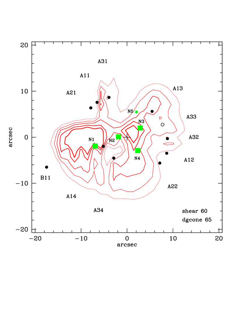
Figure 5: Mass substructure, or excess left after subtracting the smooth cluster profile from the fiducial mass reconstruction shown in Figure 1. The 5 contours, from thin to thick ones contain 8, 4, 2, 1, and 0.5% of the total reconstructed mass. The rest of the annotations are the same as in Figure 1.

Our order-of-magnitude estimate can be compared to the results of $N\!$-body simulations carried out by Randall et al. (2008), who modeled the Bullet Cluster. For the specific geometry and parameters of that cluster, and assuming $\sigma/m=0.02$ cm² gm^-1, the separation between the stellar and dark matter in the sub-cluster can be read off from their Figure 5, as $\;\hbox{\hbox to0.0pt{\raise 1.82986pt\hbox{$<$}\hss}\lower 2.79857pt\hbox{$\sim$}}\;2$ kpc. This is smaller than the separation we get for the parameters assumed in eq. 4. The main difference between the two estimates is due to the nature of the encounters in the two cases. In the Bullet Cluster, the two merging clusters made one passage past each other, so that the sub-cluster spent little time in the dense core region of the larger cluster. For the Bullet Cluster, the current separation of the sub-components is 720 kpc. A merger velocity of 4700 km s^-1 (following Randall et al., 2008) gives an encounter time of $2.3\;10^{8}$ yrs. The velocity may well be significantly lower (Springel & Farrar, 2007). But Randall et al. (2008) report that velocity of $\sim$ 2800 km s^-1 would not greatly change their results.

In the scenario we outlined above, the galaxies have been orbiting the inner cluster core for about a Hubble time. Also, $r\sim 100$ kpc is a more appropriate value for the Bullet Cluster. Taking these in to account, eq. 4 gives $d\sim 0.1$ kpc, comparable to their estimate of $\;\hbox{\hbox to0.0pt{\raise 1.82986pt\hbox{$<$}\hss}\lower 2.79857pt\hbox{$\sim$}}\;2$ kpc. Thus, the Bullet Cluster itself is a (limited) test of eq. 4.

This comparison with the Bullet Cluster demonstrates that the longer duration of the encounter and smaller distances in our scenario give rise to a larger separation, more likely to be detected.

2 The Cluster Abell 3827

Abell 3827 is rather unique; it is a nearby example of a multiple galactic cannibalism in progress, where the massive central ellipticals are closely surrounded by lensed images. The cluster’s dynamical state, its proximity to us, and the fortuitous lensing configuration make it a prime candidate for detecting any displacement between the dark and visible matter due to non-zero dark matter scattering cross-section.

In this paper we use strongly lensed images to reconstruct the mass distribution in the core of Abell 3827. As we will show, the core contains a galaxy whose visible and total mass are apparently separated by a few kpc. One possible interpretation of this result is the scenario described in the previous Section. The cluster’s lensing features were recently discovered by Carrasco et al. (2010), whose findings we summarize below.

Abell 3827 ($z\approx 0.1$) appears to be in the last stages of merger (Carrasco et al., 2010). The outer cluster looks smooth and relaxed, and there are no significant secondary galaxy concentrations. The core of the cluster contains five ellipticals, called $N1-N5$, within $\sim 15$ kpc of the centre, which appear to be in the process of spiraling inwards to form a single central galaxy. These ellipticals have probably undergone several orbits around the centre and have been tidally stripped, as evidenced by the extended $1^{\prime}.3\,\times\,1^{\prime}$ diffuse light around the core.

Carrasco et al. (2010) estimate the velocity dispersion of the cluster to be $1142\pm 125$ km s^-1, making Abell 3827 a rather massive cluster. The relative radial velocities of $N1-N3$ are within 400 km s^-1 of each other. The velocity of $N4$ is about $-1000$ km s^-1 compared to the systemic velocity. $N5$ is probably not a part of the cluster core because its velocity is about $+4000$ km s^-1 and its magnitude is $\sim 2$ fainter compared to that of the other four ellipticals.

The cluster core lenses (at least) two background sources; the main source, at $z=0.204$, is extended and consists of at least three knots, $A_{1},A_{2},A_{3}$. All three appear to be lensed into quads, but in one quad only three images are identified, and in another, only two. The second source, at $z=0.408$, forms a single arc; a counter arc may be lost in in the glare of the ellipticals. Based on their spatial distribution, the images of the quads can be labelled by their time order, even though time delays have not been measured (cf. Saha & Williams, 2003). Accordingly, we will write $A_{ij}$ to mean the $j$th arriving image of the $i$th knot within source $A$. The images to the North-East of the cluster’s centre of light are the 1st arriving ones; the two sets of images in the West are (clockwise) the 3rd and 2nd arriving, and finally the images to the South-East are 4th arriving. The 2nd and 3rd arriving images are close together and form a nearly merging pairs across the critical curve.

3 Mass reconstructions

3.1 Free-form vs. fixed-form

One can loosely divide the lens modeling methods into two categories, depending on the prior information they use. The fixed-form methods assume that mass follows light, and parametrize this relation with a handful of scalings. Free-form methods use different types of priors; most notably they do not require that mass trace light.

The authors of the discovery paper, Carrasco et al. (2010) carried out a lensing mass reconstruction using LENSTOOL, a fixed-form method (Jullo et al., 2007). The reconstruction reproduces the positions of only 5 of the 10 images well. The mean scatter between observed and recovered images is less than $0^{\prime\prime}.8$, while the astrometric uncertainty is $0^{\prime\prime}.2$. Overall, the mass model has $\chi^{2}\sim 17$ per degree of freedom, indicating that there is additional information in the astrometry.

This is not surprising; the dynamical state of the cluster core is probably unsettled, so it is quite possible that light does not follow mass. This, combined with fact that Abell 3827 has a relatively large number of lensed images—ten—makes a free-form reconstruction a logical choice.

We use a free-form reconstruction method, PixeLens (Saha & Williams, 2004; Coles, 2008). The reconstruction is done in a circular window, which is divided into many equal-sized square pixels. The mass within each pixel is uniformly distributed but each pixel’s mass value is allowed to vary independently of others. PixeLens takes advantage of the fact that the lensing equation is linear in the mass pixels and in the coordinates of the source, and so it is relatively straightforward to come up with solutions that reproduce image positions exactly. In fact, since the unknowns outnumber the knowns (coordinates of the lensed images) by a large factor, an infinity of solutions are possible. PixeLens generates a user-specified number of individual models, according to a weak and adjustable prior of which the ensemble average is considered in this paper. The prior and the model-sampling technique are motivated and explained in detail in the above papers, so here we just remark on two points that are important for the modelling.

First, along with the image positions, a notional centre must be given. The default behaviour of PixeLens is to require the local density everywhere to point at most $45^{\circ}$ away from the centre. In this work we increase the allowed angle (called dgcone for “density-gradient cone”) somewhat, typically to $65^{\circ}$. This allows more substructure, as appears to be demanded by the data.

Second, to account for the mass exterior to the modeling window, PixeLens can add external shear of any magnitude. The shear axis can be within $45^{\circ}$ of a user-specified shear direction, denoted by shear. We typically set shear 60 —on the basis of the axis of the diffuse light on arcminute scale around the cluster core— which permits any shear orientation from $15^{\circ}$ to $105^{\circ}$.

The version of the lens-reconstruction software used is included as an online supplement. Other examples of free-form techniques for cluster lenses are described in Liesenborgs et al. (2007) and Coe et al. (2008).

3.2 Fiducial reconstruction

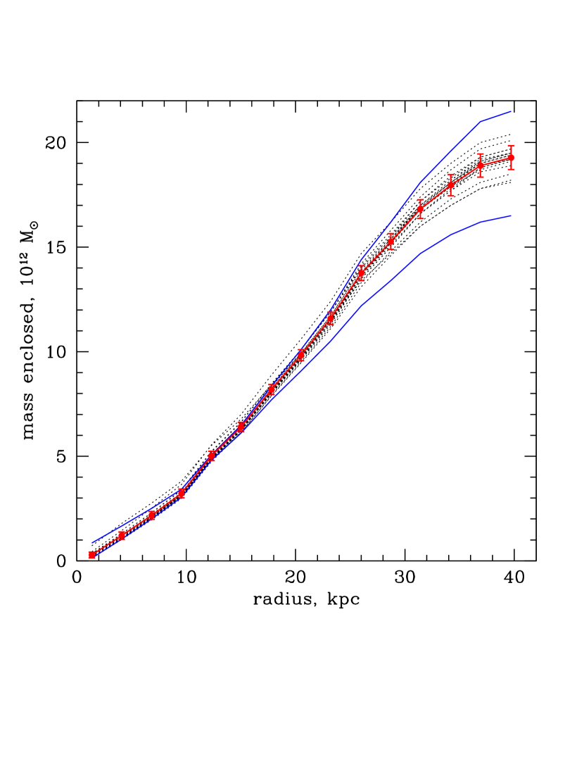
Figure 2: Mass enclosed as a function of distance from centre. The central thick red line with points and errorbars represents the average and rms dispersions of 18 reconstructions shown in Sections 3.3 and 3.4. The think black dotted lines are the 18 individual reconstructions. Our fiducial reconstruction is indistinguishable from the average. The two blue solid flanking lines enclose 90% of the 500 individual mass models of the fiducial reconstruction.

To start with, we create a reference, or fiducial reconstruction. It uses all the 10 images identified by Carrasco et al. (2010). As the centre we use the centre of light (also the centre of their Figure 2 frame), which is about $2^{\prime\prime}$ West of N2.

At the redshift of the cluster, $z=0.1$, the critical surface mass density for sources at infinity is $\Sigma_{\rm crit}=0.953$ gm/cm², and $1^{\prime\prime}$ corresponds to 1.93 kpc, for $\Omega_{m}=0.3$, $\Omega_{\Lambda}=0.7$, and $h=0.67$. The diameter of the reconstruction window was set to 29 pixels, with the scale of $1.43^{\prime\prime}$/pixel, so the angular and physical size of the window are about $40^{\prime\prime}$ and 77 kpc, respectively.

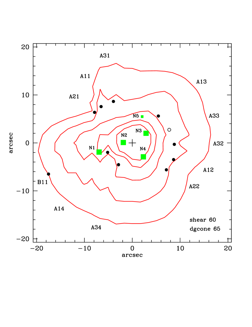
Figure 1: Fiducial mass reconstruction. The map is an average of 500 individual mass maps. Contours of equal projected mass density are at 0.9, 1.3, 1.7, 2.1 and 2.5 of $\Sigma_{\rm crit}$, where $\Sigma_{\rm crit}$ is the critical density for $z_{l}=0.1$ and sources at infinity. Images identified by Carrasco et al. (2010) are marked with black solid dots, and labeled at the periphery of the figure. $A_{ij}$ means the $j$th arriving image of the $i$th knot within source $A$. The empty black circle is the $A_{33}$ image that the present authors identified from the observed image. It is not used in the fiducial but it used in some later reconstructions. Green squares are ellipticals; N5 is marked with a smaller symbol because it is probably not a part of the cluster core. At the redshift of the cluster, $1^{\prime\prime}=1.93\;h^{-1}_{0.67}$ kpc.

The fiducial PixeLens reconstruction is shown in Figure 1; the mass density contours are spaced by $0.5\,\Sigma_{\rm crit}$. The map is an average of 500 individual models. (The mass map is not sensitive to the number of individual models in the ensemble as long as it is greater than $\sim 100-200$, the pixel size within the range $1.25^{\prime\prime}$-$2^{\prime\prime}$ per pixel, or the orientation of the reconstruction window with respect to the cardinal directions.) Figure 2 is a plot of mass enclosed as a function of radius. Our fiducial reconstruction is indistinguishable from the average of 18 reconstructions discussed in Sections 3.3 and 3.4, and shown as the red thick line. The thin dotted lines are all the 18 models, and the errorbars represent their rms dispersion. The two blue solid flanking lines enclose 90% of the 500 individual mass models of the fiducial reconstruction. Note that at large radii, i.e. outside the images, the enclosed mass begins to level off since the image positions do not require any mass at those radii. However, the 90% errorbars are fully consistent with the density profile continuing on with the same slope as at smaller radii.

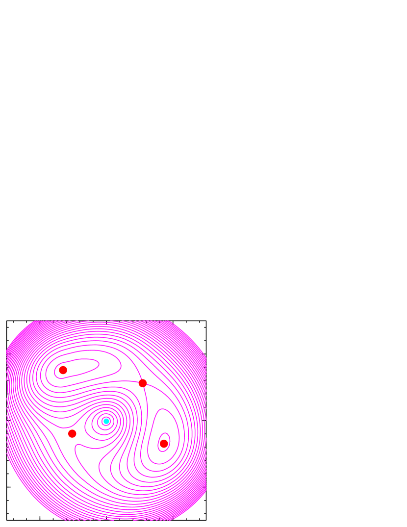
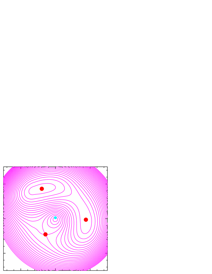
Figure 3: Arrival time surfaces of PixeLens fiducial reconstructions of sources $A_{1}$ and $A_{3}$.

Figure 3 shows the arrival time contours of the $A_{1}$ and $A_{3}$ knots of source $A$. From the contours, we see that the model indicates extra images appearing next to the first arriving image of $A_{1}$. These may be spurious, or may actually be present, depending on the local mass substructure. They do not, however, affect the larger-scale features of the mass maps, which are the focus of this paper. The plot of arrival-time contours also provides a simple model for the ring-like extended image (cf. Saha & Williams, 2001) which in this case arises from the extended source $A$. Detailed comparison would, however, be very difficult because the ring is faint and in many places overlaid with the light from the ellipticals.

We have not attempted to use the arc $B$ as a lensing constraint, since it has no identified counter image. In principle it is possible to extract some strong-lensing information from this arc. If pointlike features could be identified, they could be put in as multiple-image constraints in the usual way. Another possibility would be to assume two fictitious image positions along the arc, which in models would have the effect of forcing a critical curve to pass through the arc.

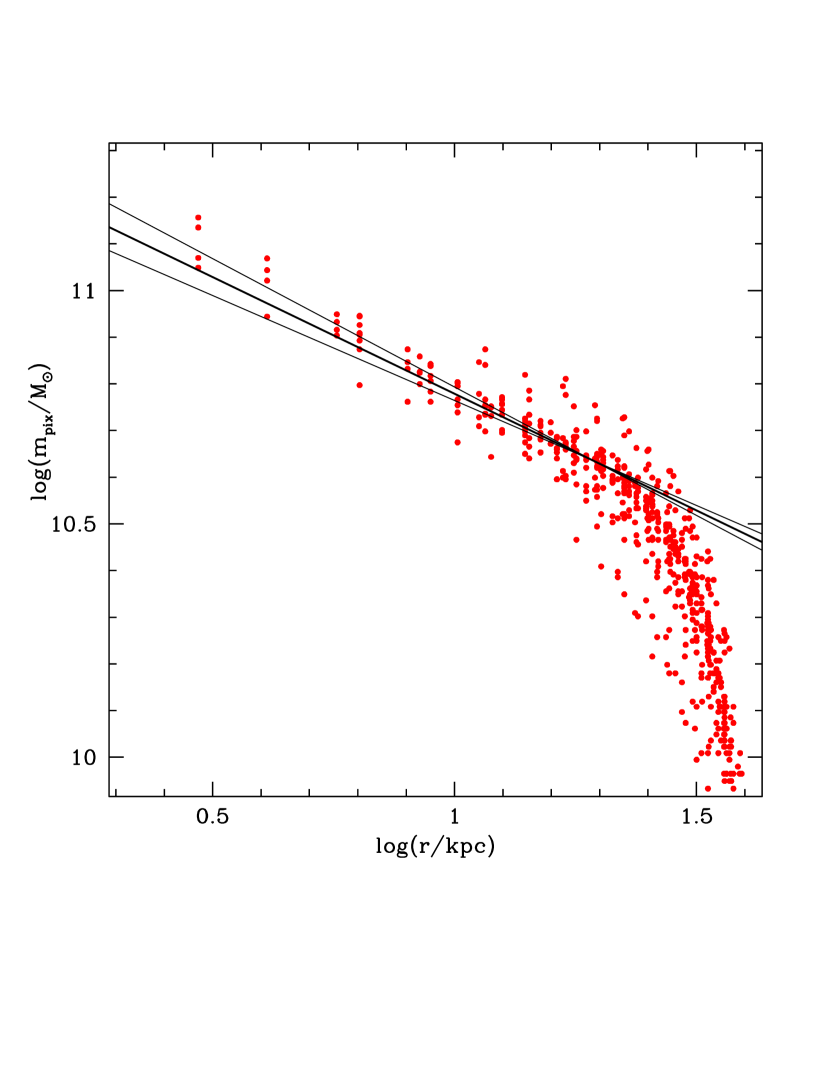
Figure 4: Pixel mass vs. distance from centre for the fiducial reconstruction — each dot represents a mass pixel. The outermost multiple image is at a projected radius of 20 kpc. (The arc $B_{11}$ is at 37 kpc, but no counter-images have been identified.) There is thus no new strong-lensing information beyond 20 kpc, and PixeLens puts very little mass into pixels further out. The three straight lines have log-log slopes of -0.45, -0.5 and -0.55. To reveal the mass substructure, or excess above the smooth cluster profile, the slope of -0.5 was subtracted from PixeLens ensemble average maps; the normalizations were chosen as described in Section 3.2.

The mass contours in Figure 1 show deviations from circular symmetry, which are due to mass inhomogeneities in the lens. We isolate these by subtracting a smooth component, as follows. Figure 4 shows pixel mass as a function of the distance from the centre of the fiducial reconstruction. As already mentioned when discussing Figure 2, the lack of lensing constraints beyond about 20 kpc leads PixeLens to put very little mass into those pixels; so the tapering off of points in Figure 4 is an artifact. The average projected density profile slope where the images constrain the mass well, i.e. around $\sim 6^{\prime\prime}-24^{\prime\prime}$, is $d\ln\Sigma(R)/d\ln R\approx-0.5$, and is representative of most mass maps in this paper. This is shown as the thick straight line in this log-log plot; the other two lines have slopes of $-0.45$ and $-0.55$, and represent the reasonable range of possible power-law slopes. To isolate the mass inhomogeneities we subtract circularly symmetric density profile of slope $-0.5$ from the reconstructed mass maps; a change of $\pm 0.05$ in the assumed smooth profile slope would not have made a significant difference. The normalization of the subtracted profile is adjusted such that the contours of substructure, or the excess mass density left after the subtraction of the smooth cluster profile, contain 0.5, 1, 2, 4 and 8 % of the total mass within the full $40^{\prime\prime}$ window. This normalization is calculated separately for each mass map and each of the five contour levels.

Figure 5 shows the five contour levels of the mass substructure, as red solid lines; thicker lines represent contours of smaller enclosed mass. Images are shown as black solid dots, and labeled at the periphery of the figure. The arc $B_{11}$ has no detected counter images. Image $A_{33}$ was not identified by Carrasco et al. (2010), but looking at their Figure 2, the present authors feel $A_{33}$ is the location of that image. It is not used in the fiducial reconstruction but is used in some other ones. Galaxies are denoted by green squares and labeled as in Carrasco et al. (2010); $N5$ is a smaller square because the galaxy is probably background and less massive.

Figure 5 shows that the mass substructure does not trace the visible galaxies, an indication that the cluster core is not in equilibrium, but is dynamically disturbed. There is one dominant mass clump, to the North East (upper left) of galaxy $N1$, but not centered on $N1$. This clump is the main subject of the paper, and we will refer to it as the NE-$N1$ clump. A smaller clump is between galaxies $N3-N4$, and seems to be avoiding $N2$. The following sections will demonstrate that even though the details of the reconstructions differ, the main features of this fiducial mass map, and most importantly the existence and location of NE-$N1$ clump, and the lack of mass associated with $N2$, are robust to changes in priors, centre of the reconstruction window, and, to some degree, the subsets of images used in reconstruction.

3.3 Effect of priors used in reconstruction

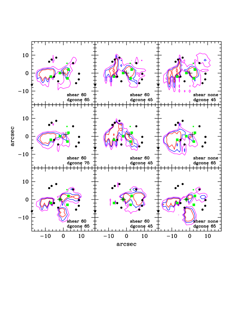
Figure 7: Mass substructure left after subtracting smooth density profiles from PixeLens mass maps shown in Figure 6 (see Section 3.2). The density contours containing 0.5, 1 and 2% of the total reconstructed mass are plotted as red, blue and magenta curves, respectively.

Figure 7 shows maps of substructure mass contours for nine reconstructions. The image set used is the same as in the fiducial case, but the priors are different. The assumed values of dgcone, and shear are shown in each panel. Since the cluster core is most likely not in equilibrium, we tried three different lens centres. The fiducial one is called $C0$, and was identified by Carrasco et al. (2010) as the cluster’s centre of light; it sits between $N2$ and $N3$. Centre $C1$ is shifted by $(+1^{\prime\prime}.5,+1^{\prime\prime})$ from $C0$ and is close to $N3$. Centre $C2$ is shifted by $(-1^{\prime\prime}.875+0^{\prime\prime}.08)$ with respect to $C0$; it coincides with the location of galaxy $N2$, the central-most elliptical in the core. The three choices for the lens centre are used in the reconstructions of the three rows of Figure 7, respectively. Their location is marked with a cross. (We remark again that the lens centre in PixeLens is needed because the density gradients, used for dgcone, are calculated with respect to the lens centre. The other utility of the lens centre will be put to use in Section 3.7.)

Figure 7 shows that all reconstructions, with the possible exception of the middle panel of the third row, require a mass lump to the NE of galaxy $N1$. The size and position of the lump vary between panels, but in none of these is the lump centered on $N1$; it is always to the upper left of that galaxy. The other common feature is that $N2$ has relatively little excess mass associated with it. The nearby mass clump sometimes encompasses $N3$ or $N4$, but not $N2$.

3.4 Effect of image subsets used in reconstruction

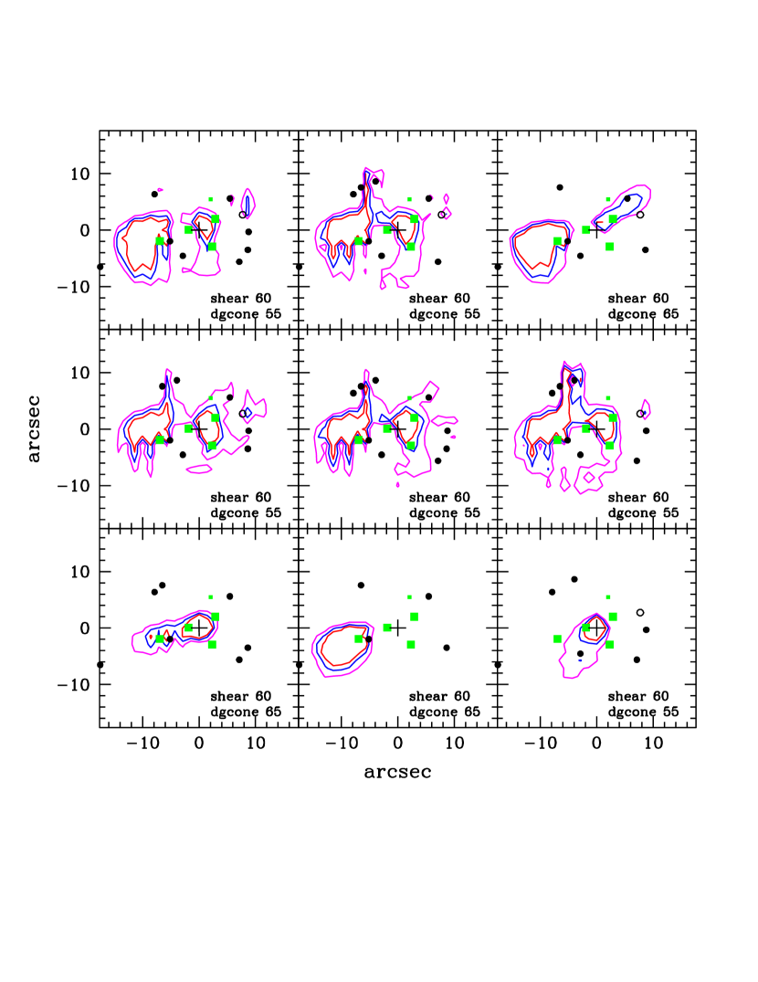
Figure 9: Similar to Figure 7, i.e. mass substructure, but for PixeLens maps shown in Figure 8.

Figure 9 shows the effect of leaving out some of the lensed images from the reconstruction. The images plotted in each panel are the only ones used in the corresponding reconstruction. The lens centre is always $C0$, and the PixeLens priors are shown in each panel. Most changes to the image set makes little difference to the global features of the recovered mass maps, and specifically the NE-$N1$ mass clump.

Since this mass clump is of primary interest for us, we examine its dependence on the images more closely. From this Figure, and other reconstructions not shown here, we know that the single most important image that determines the location of the clump near $N1$ is image $A_{14}$. In the lower right panel $A_{14}$ was not used, and the mass clump moved to a different, lower, or more Southerly, location. In that reconstruction, both the mass distribution and the image configuration have an approximate bilateral symmetry, with the axis inclined by $\sim 60^{\circ}$ to the $+x$-axis. The location of $A_{14}$ predicted by such a bilaterally symmetric mass distribution would have been very close to the observed $A_{34}$. However, the observed $A_{14}$ is about $4^{\prime\prime}$ clockwise from $A_{34}$.

To make that happen, one needs a large mass clump roughly where PixeLens puts the NE-$N1$ clump. This can be understood in terms of the arrival time surface. $A_{14}$ is a saddle point image. A sufficiently large mass just outside of the image circle will create a local bump in the arrival time surface and a saddle point will be created between it and the centre of the lens.

In Section 4.1 we will present additional arguments to show why $A_{14}$ requires a large mass to exist beyond the location of galaxy $N1$.

One might be tempted to say that $A_{14}$ has been misidentified, and is actually much closer to $A_{34}$. If that is assumed, the reconstructed mass and observed galaxy positions bear no correspondence to each other, as shown in the lower right panel of Figure 9. Furthermore, the imaging data as presented in Carrasco et al. (2010) shows a definite, though faint smudge at the location of $A_{14}$. We conclude that $A_{14}$ is real, and hence the true mass distribution is close to what our fiducial reconstruction looks like.

3.5 Properties of the NE-$N1$ mass clump

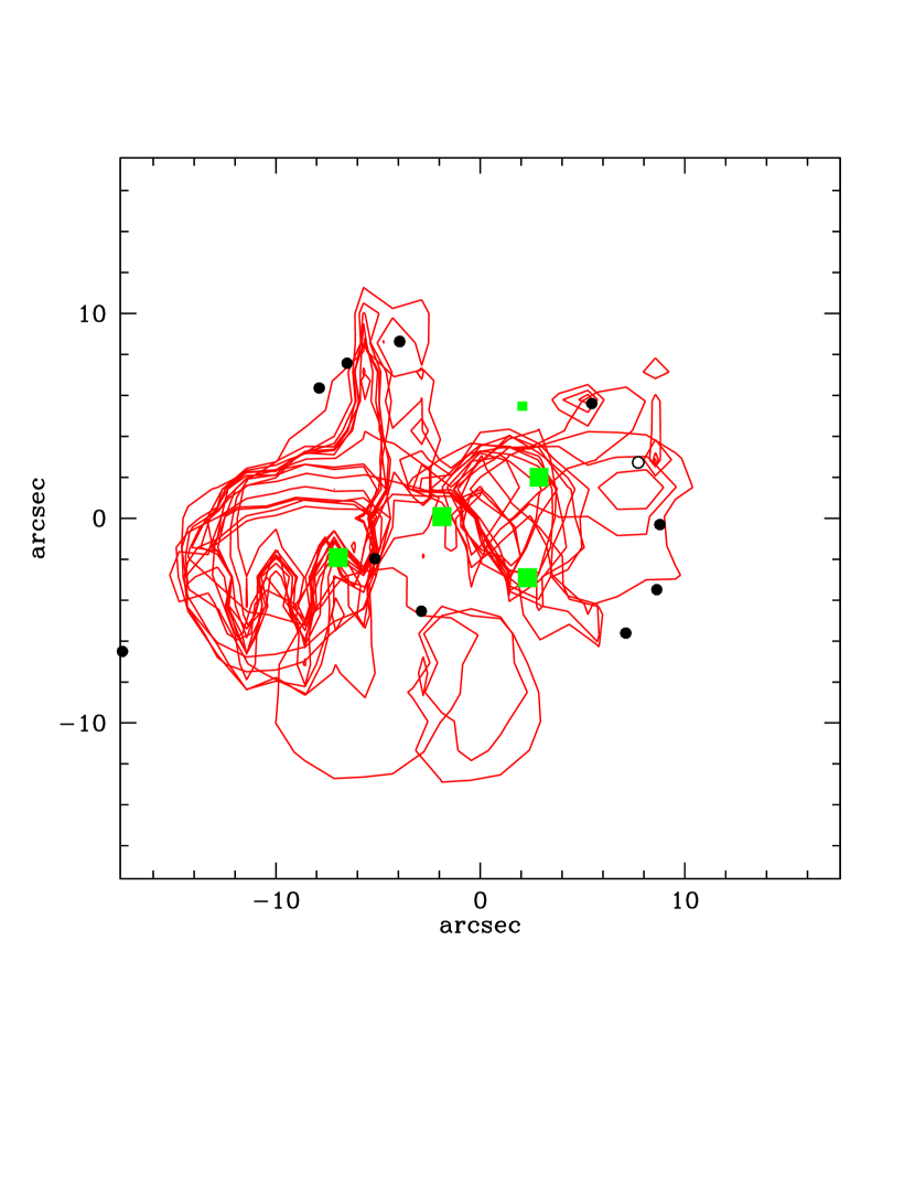
Figure 10: All eighteen reconstructions from Figures 7 and 9, but only one contour per reconstruction is shown, the one enclosing 1% of the total mass. As before, galaxies are represented by green squares, lensed images are black dots. This plot highlights the features common to all reconstructions: the massive NE-$N1$ mass clump, and the secondary clump around galaxies $N3$ and $N4$, which avoids $N2$.

The mass substructure, i.e. the excess left after subtracting the smooth cluster profile, of all eighteen reconstructions of Figures 7 and 9 are superimposed in Figure 10. For clarity, we plot only the contours enclosing 1% of the total mass in every reconstruction. The figure highlights the features common to most reconstructions: the massive NE-$N1$ mass clump, and the secondary clump around galaxies $N3$ and $N4$, which avoids $N2$.

The main goal of the paper is to estimate the lower limit on the dark matter cross-section using eq. 4 as applied to galaxy $N1$ and the NE-$N1$ mass clump. In this section we estimate the parameters associated with the NE-$N1$ clump, namely, its mass, $M_{dm}$, size, $s$, and distance from $N1$, $d$, and give a measure of dispersion in these properties between reconstructions.

Figure 10 gives a visual impression of the systematic uncertainties in our reconstructions. Because the shape and location of the NE-$N1$ clump is not exactly the same in various reconstructions, there is no unique way of quantifying its average properties and estimating the dispersion in these properties between the various mass maps.

We chose to use an iso-density mass substructure contour to define the clump, and the corresponding mass excess within that contour as the clump’s mass, its center of mass as the center of the clump, and the enclosed area, $A$, to define the size of the clump, i.e. $s=(A/\pi)^{1/2}$. First, we need to decide what to take as the boundary of the clump. In most reconstructions, including the fiducial one, the mass substructure contours containing 0.5 and 1% of the total mass are disjointed, and enclose separate mass clumps, while the contours containing 4 and 8% of the total mass form one contiguous region. This suggests that $\sim 1\%$ of the total recovered mass is in the individual clumps, therefore we take the closed 1% contour located to the NE of the $N1$ galaxy as defining the clump.

Two of the reconstructions, the bottom middle in Figure 7 and the bottom right in Figure 9 have no excess mass at 1% level in the vicinity of $N1$, so we exclude them. With these choices, the average and rms dispersion in the mass of the NE-$N1$ clump based on the 16 maps is $M_{dm}=(1.22\pm 0.44)\;10^{11}M_{\odot}$, its distance from the centre of the elliptical $N1$ is $d=2.68^{\prime\prime}\pm 1.08^{\prime\prime}$, and its size $s=4.28^{\prime\prime}\pm 2.46^{\prime\prime}$. Our fiducial reconstruction gives $M_{dm}=1.47\;10^{11}M_{\odot}$, $d=2.50^{\prime\prime}$, and $s=4.11^{\prime\prime}$, all of which are within the rms of the 16 maps, so when estimating $\sigma/m$ in Section 5 we will use the fiducial values.

We also need to estimate $r$, the clumps distance from the cluster centre. Equation 3 assumes that the centre of the elliptical galaxy and the centre of its displaced dark matter halo are equidistant from the cluster centre, i.e. $r_{st}\approx r_{dm}$ since the displacement $d$ is small. Therefore we take $r=r_{st}\approx 7.2^{\prime\prime}$, same for all reconstructions. The uncertainty in $r$ comes from the uncertainty in the location of the cluster centre. In Section 3.7 below we show that the latter is of order $1^{\prime\prime}-2^{\prime\prime}$, which translated into a fractional error, which is smaller than that in the other two relevant lengths, $d$ or $s$.

While the errors in the estimated properties of the NE-$N1$ mass clump are relatively small, $\;\hbox{\hbox to0.0pt{\raise 1.82986pt\hbox{$<$}\hss}\lower 2.79857pt\hbox{$\sim$}}\;50\%$, we stress that these are not the main sources of uncertainty in estimating the parameters of the dark matter particle cross-section, $\sigma/m$. The dominant sources of uncertainty are the unknown dynamics of the cluster, the evolution in cluster core’s density profile slope, and the galaxy orbit shape, especially that of elliptical $N1$ (see Section 1), and cannot be quantified using lensing data. To properly address these one would need to carry out a series of N-body simulations with a range of initial conditions.

3.6 Effect of image position uncertainties

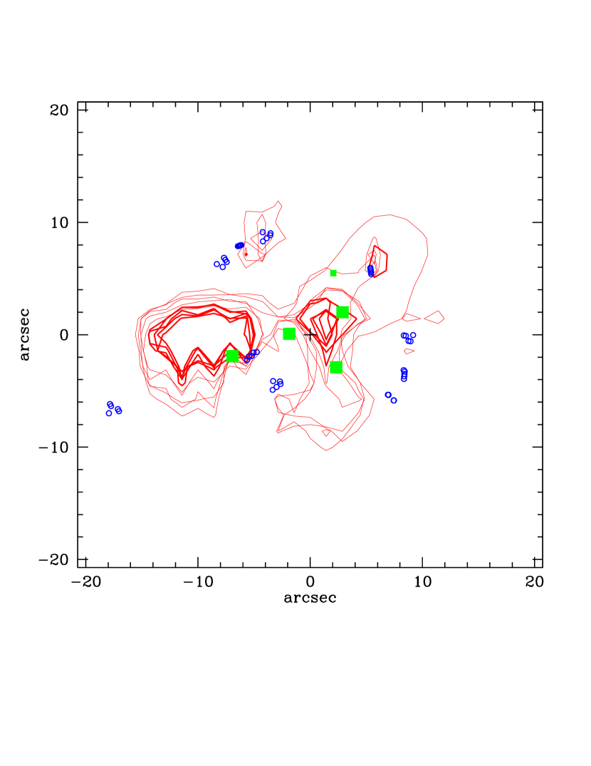
Figure 11: Five overlaid fiducial reconstructions, except lens image positions have been randomly scattered within $0^{\prime\prime}.5$ of the true positions, and are shown as blue empty circles. Two sets of mass substructure contours per reconstruction are plotted, at 0.5% (thick lines) and 2% (thin lines). The two main features common to all reconstructions are robust against astrometric uncertainties.

Based on their observations, Carrasco et al. (2010) quote image astrometric uncertainty of $0^{\prime\prime}.2$. Since PixeLens reproduces image positions exactly, we need to check if astrometric errors could have affected our results. Here we redo the fiducial reconstruction but randomly shift the observed images within $\pm 0.5^{\prime\prime}$ of their true positions. Five realizations are shown in Figure 11. To reduce run-time, we used 300 models to create an ensemble, instead of the usual 500. Since all five reconstructions look very similar and have small rms dispersions ($M_{dm}=(1.39\pm 0.23)\;10^{11}M_{\odot}$ and $d=2.77^{\prime\prime}\pm 0.17^{\prime\prime}$), smaller than the ones presented in the Section 3.5 we conclude that astrometric errors have not affected our results.

3.7 Centre of mass of the cluster

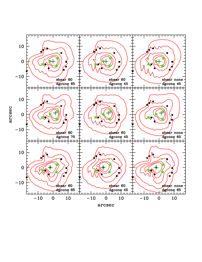
Figure 6: PixeLens mass reconstructions using different priors and lens centres. The values of shear and dgcone are indicated in each panel; the centre of each reconstruction window is marked with a cross, and is different in each of the three rows. The top row assumes the fiducial lens centre. The whole fiducial lensed image set (10 images) is used in all nine reconstructions; images are marked with black solid points. The top left map is the fiducial map. The mass density contours are at 0.9, 1.3, 1.7, 2.1, and 2.5 of critical surface mass density for lensing for sources at infinity.

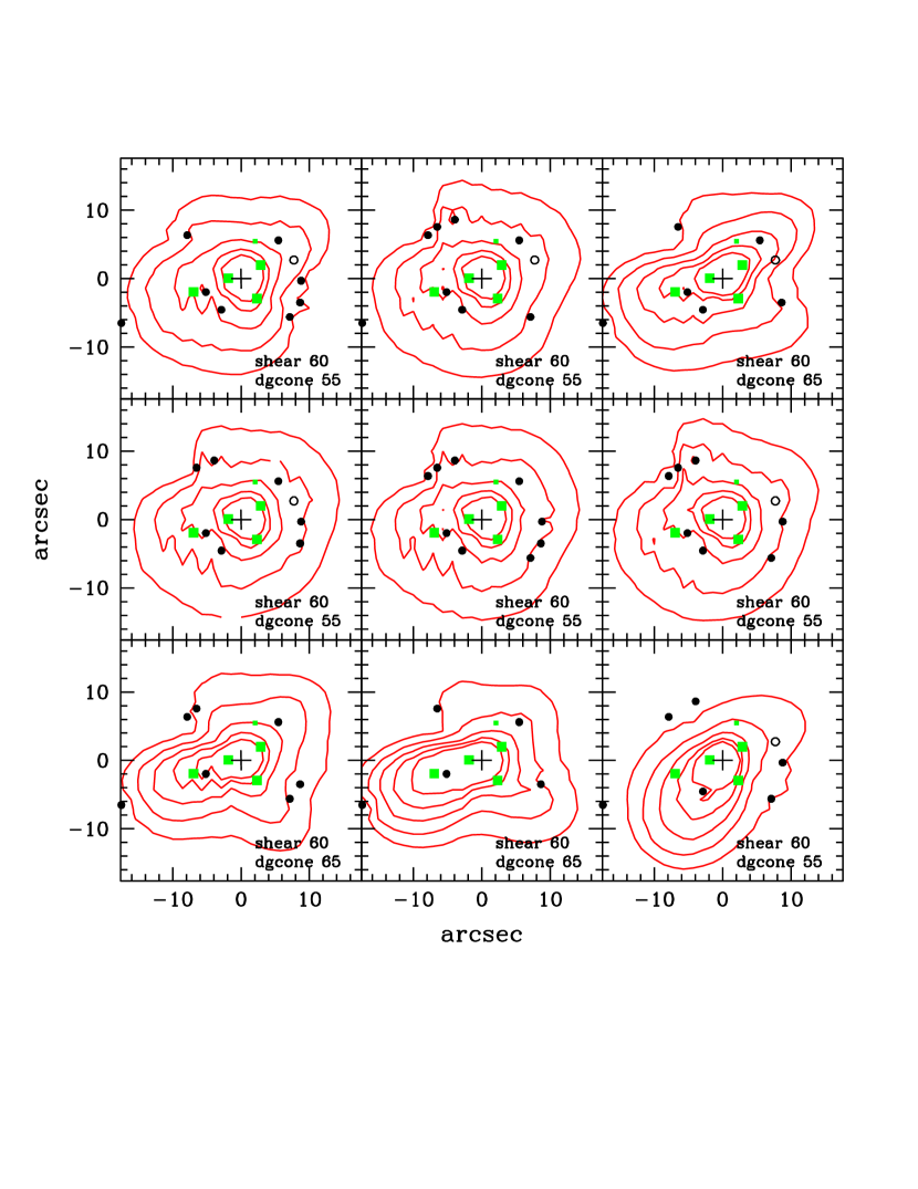
Figure 8: Similar to Figure 6, but using different sets of lensed images, which are indicated in each panel. The lens centre is the same in all nine reconstruction (same as fiducial), and is marked with a cross.

In addition to the NE-$N1$ clump, the other notable feature of the reconstructions is that regardless of the input model parameters (see Figures 5-11) there is very little mass excess associated with $N2$, the centrally located elliptical galaxy. This suggests that the peak of the mass distribution is not very close to $N2$. Here we ask which one of our three trial centres, $C0$, $C1$, or $C2$ comes closest to the true cluster centre, defined as the location of the largest mass concentration. We use the following procedure.

A PixeLens pixel can assume any mass value provided it agrees with the image positions and priors, like dgcone and shear. If there is no smoothing, the resulting maps usually show a lot of fluctuations between neighbouring pixels. To avoid that, we impose a nearest neighbour smoothing constraint by requiring that a pixel cannot have a mass value larger than twice the average of its eight neighbours. The only exception to this rule is the pixel at the centre of the reconstruction window, which has no imposed upper bound. It is reasonable to suppose that the closer the reconstruction centre is to the real centre, the more mass the central pixel will contain.

From our total (not substructure) mass maps we calculate the fraction of total mass contained in the central pixel. For the centres $C0$, $C1$ and $C2$ we calculate that percentage of mass as $1.47\pm 0.25$,  $2.47\pm 0.22$,  and $0.79\pm 0.063$ respectively. These values are averages and rms for the three sets of three maps shown in Figure 7. Recall that $C2$ is centered on galaxy $N2$, whereas $C0$ and $C1$ correspond to ’blank spots’ between $N2$ and $N3$. Since the central pixel of $C2$ contains the least mass, and has the smallest dispersion of the three cases, it supports our finding in the earlier Sections that there is very little excess mass associated with the optical light of elliptical $N2$. Of the three, centre $C1$ is closest to the largest concentration of mass in the cluster.

Finding the centre of the cluster is not the main goal of the paper, however this Section demonstrates that the uncertainty in the location of the centre is of order of $1^{\prime\prime}-2^{\prime\prime}$, and hence smaller than fractional uncertainties in the other length measurements entering eq. 4, i.e. $d$ and $s$, therefore when estimating $r$ it is reasonable to use $C0$ as the centre of the cluster, as we have done in Section 3.5.

3.8 Adding point masses at the locations of galaxies

To further test the robustness of the NE-$N1$ mass clump we carry out a reconstruction where PixeLens is allowed to add point masses at specified pixel locations. In other words, we allow some pixels to override the nearest neighbour constraint described in Section 3.7.

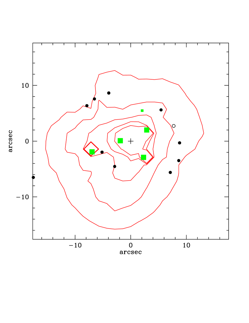
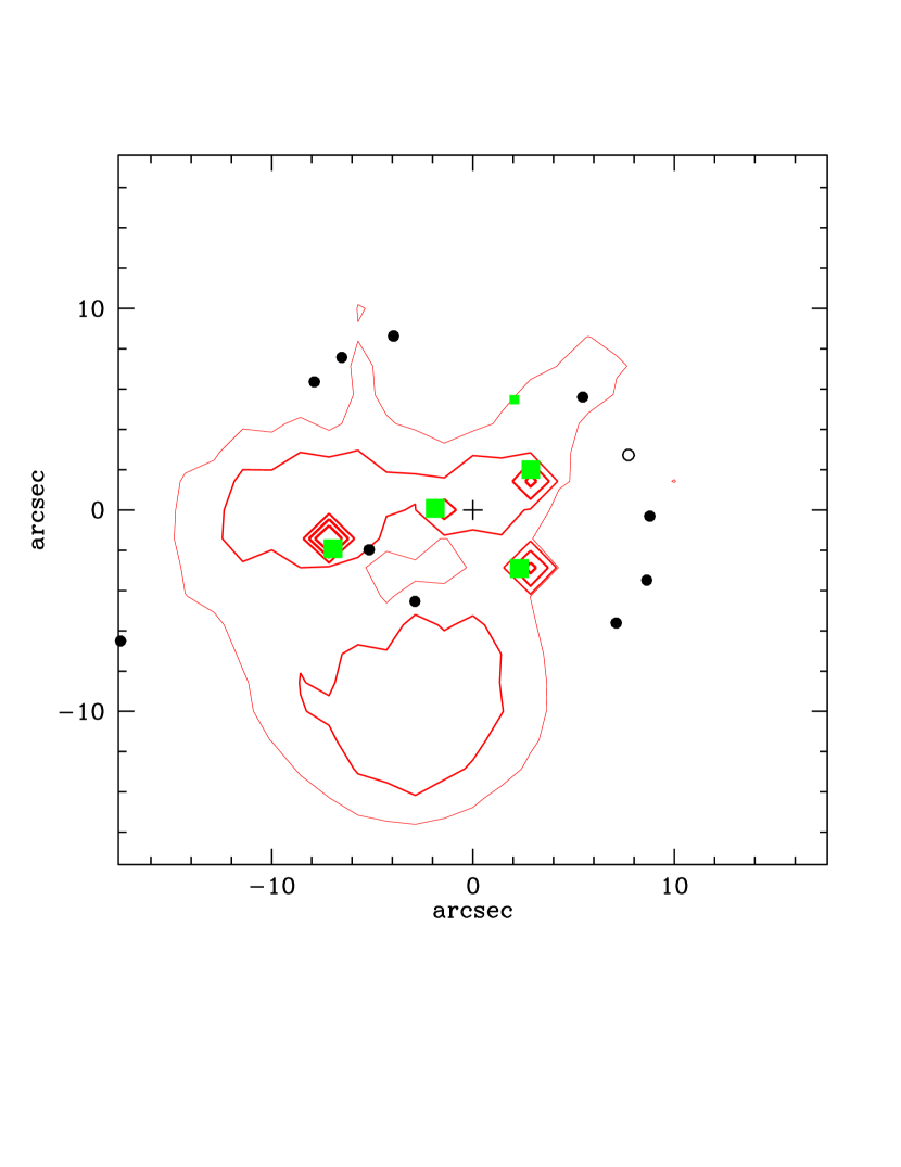
Figure 12: Mass density contours (left) and substructure left after subtracting smooth cluster profile (right) of PixeLens fiducial reconstruction, except here PixeLens was specifically allowed to put extra mass at the locations of the four main ellipticals. This extra mass is seen as density contours around green squares representing $N1-N4$. In the left panel the mass countour levels are at 0.9, 1.3, 1.7, 2.1, and 2.5 of critical surface mass density for lensing for sources at infinity, while on the right the contour levels of the mass substructures are at 0.5, 1, 2, 4 and 8% of the total mass. Note that the 1% contour delineates the NE-$N1$ mass clump; see Section 3.8 for details.

We chose pixels containing the observed galaxies $N1$-$N4$, and use PixeLens command ptmass x y area1 area2, where x and y is the location of the point mass, and area1 area2 are the lower and upper limits on the area enclosed by its Einstein ring. We used $0$ and $20$ arcsec² as representative values for mass associated with individual galaxies. Figure 12 shows the results. The contour levels of the mass substructure are the same as before, at 0.5, 1, 2, 4, and 8% of total.

There is a substantial amount of mass associated with individual galaxies, including $N1$, but a large mass to the upper left of $N1$ is still required, as shown by the 1% substructure mass contour. In fact, the NE-$N1$ clump, without the $N1$ point mass, roughly contains $1-2\;10^{11}M_{\odot}$, similar to what we find for the fiducial reconstruction, in Section 5. Also consistent with earlier findings, is that compared to other ellipticals, $N2$ has the least amount of mass associated with it.

4 Tests using synthetic mass models

4.1 Image $A_{14}$ and the NE-$N1$ mass clump

In this section we create a series of four synthetic mass distributions that illustrate why an excess mass lump is needed where PixeLens places it, to the North East of $N1$. These synthetic maps have mass distributions similar enough to the real cluster to make the comparison meaningful. However the images produced by them do not attempt to exactly reproduce the observed images.

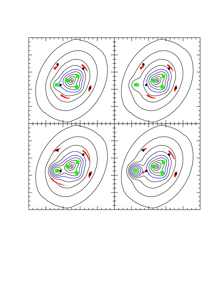
Figure 13: A series of four synthetic mass distributions designed to elucidate why free-form PixeLens reconstruction puts a massive secondary clump, the NE-$N1$ clump, outside of image $A_{14}$. Green squares are the locations of galaxies; their mass contribution can be judged by how much they distort the density isocontours of the total mass distribution, shown as black curves. The blue contour is the critical surface mass density for lensing. Red islands of points are quad images produced by these mass distributions. Black solid points represent the observed images of the $A_{1}$ knot; these are not produced by the mass distributions shown in this Figure. Notice that only in the bottom right panel, where $N1$ galaxy is made more massive and moved to the upper left, the fourth arriving images of the red quads move to the location of the observed $A_{14}$.

In Figure 13 the mass map in the upper left is roughly what Abell 3827 would look like if mass followed light, in other words, mass clumps are placed at the observed locations of galaxies $N1$-$N4$, indicated by the green squares. The blue contour has the critical surface mass density for $z_{s}=0.2$. The black solid dots are the locations of the observed images of source $A_{1}$. The four extended islands of red points mark the locations of images produced by this synthetic mass configuration. These images were selected such that the second arriving images cluster around the observed $A_{12}$. The other images were unconstrained.

The locations of the 1st, 2nd and 3rd arriving images can be relatively well reproduced by the mass-follows-light scenario. However, the 4th arriving images are consistently far from the observed $A_{14}$. This is the basic reason why mass-follows-light models do not work.

What does one have to do to (approximately) reproduce $A_{14}$? In the upper right panel of Figure 13 we move the mass clump associated with $N1$ to the left (East). The 4th arriving images are hardly affected. Next, in the lower left panel we keep the mass clump at its original position but increase its mass by $\times 6$. The configuration of images changes but the location of $A_{14}$ is still not reproduced. Finally, in the lower right panel we move the mass clump to the left and increase its mass by $\times 6$. Now the bulk of the 4th arriving images move to where the observed location of $A_{14}$. This is basically the mass distribution that PixeLens finds, with its massive NE-$N1$ clump.

4.2 Reconstructions of synthetic mass distributions with PixeLens

A further test of the veracity of PixeLens’s reconstructions is to use the images created by the synthetic mass distributions of the previous section as input for PixeLens.

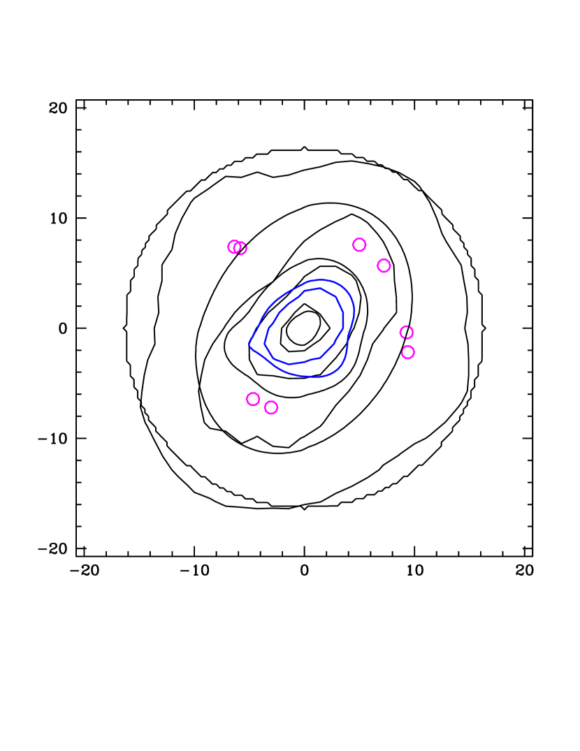
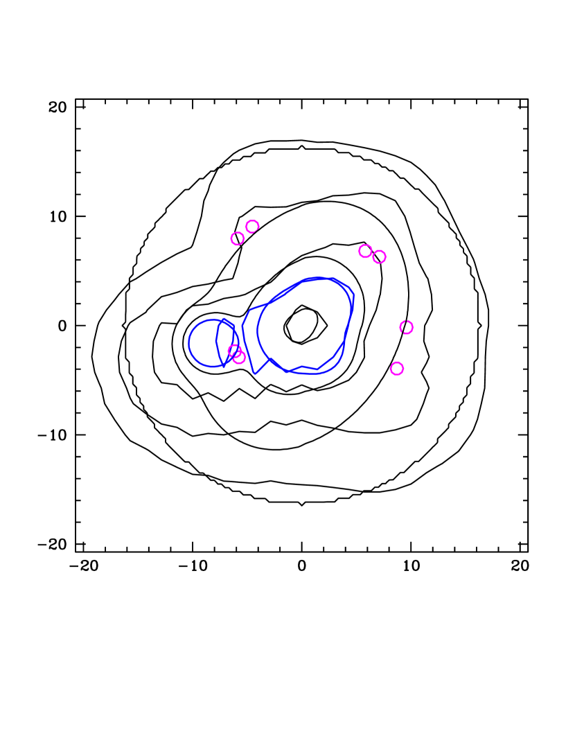
Figure 14: Known synthetic (smooth) and PixeLens reconstructed (jagged) mass contours of the lens in the upper left and the lower right panels of Figure 13, shown here in the left and right panels, respectively. The black contours are at 0.25, 0.5, 0.75 and 2 of critical surface mass density; the blue contour is at 1. The purple empty circles are the images of two quads, produced by the synthetic mass distributions and used for the reconstruction.

We use the mass distributions of the upper left and lower right panels of Figure 13. For each of these we take two quads from the red dots in Figure 13, for a total of eight images to be used as lensing constraints. The two panels of Figure 14 show the synthetic mass distributions as the smooth contours, while the jagged contours are the PixeLens reconstructions. The black mass contours are at 0.25, 0.5, 0.75 and 2 of the critical surface mass density for $z_{s}=0.2$, while the blue contour is at the critical density. The magenta empty circles are the images used in the reconstruction.

The first of the two synthetic mass models (left panel) is approximately elliptical and does not have a mass lump to the left of the centre. PixeLens recovers the mass map quite well; most importantly it does not create a fictitious massive clump near the 4th arriving image. The second synthetic mass map (right panel) does have a mass clump, and PixeLens recovers it well.

5 Dark matter cross-section

The reconstructions of the preceding Sections and the tests with synthetic lenses show that the two main features of the lensing mass reconstructions are robust. (1) The NE-$N1$ mass clump is present consistently in most reconstructions, and it is never centered on galaxy $N1$. (2) The second, less massive clump is near galaxies $N3$ and $N4$, but avoids $N2$, so that there is no excess mass associated with that central elliptical.

We interpret (1) to mean that the visible and the dark components of $N1$ are separated, and we hypothesize that the cause of the separation is the scenario described in Section 1, namely that the scattering between the galaxy’s and the cluster’s dark matter particles induced the galaxy’s halo to lag behind its stellar component. Other interpretations of the observed separation are discussed in Section 6. Conclusion (2) also speaks to the dynamically disturbed nature of the cluster core, though there is not enough information to speculate what happened to the halo of $N2$ and how the mass clump is related to the nearby $N3$ and $N4$.

We now concentrate on (1), and estimate $\sigma/m$ from eq. 4 and the parameters based on the reconstructions presented in Sections 3.3 and 3.4 and summarized in Section 3.5. We do not consider the rms dispersions quoted in that Section here, because the main source of uncertainty is not in the measured properties of the NE-$N1$ clump, but in the dynamics of the cluster. For a conservative lower limit on $\sigma/m$ we want to use the smallest linear distances, $r$, $s$, and $d$ consistent with the reconstruction, so we use the sky projected quantities, and make no attempt to estimate the corresponding three-dimensional values.

To obtain $M_{co}$ we measure the projected mass within $r$ from Figure 2 and halve it to account for the core being a sphere instead of a long tube; $M_{co}\sim 2.9\;10^{12}M_{\odot}$.

One major source of uncertainty is related to the quantity $M_{co}/r^{2}$ entering eq. 4. First, if $M_{co}/r^{2}$ depends on radius, i.e. distance from cluster center, then the unknown shape and ellipticity of $N1$’s orbit and hence how it ‘samples’ $M_{co}/r^{2}$ becomes an issue. Second, the radial dependence of $M_{co}/r^{2}$ may well be time dependent. From our lensing reconstruction we can measure how this quantity scaled with radius at the present epoch. The projected $\Sigma\propto R^{-0.5}$, which implies that the space density $\rho\propto r^{-1.5}$, and mass enclosed $M_{co}\propto r^{1.5}$, so $M_{co}/r^{2}\propto r^{-0.5}$. This is a relatively weak radial dependence, but it does not tell us much about the temporal dependence. In future work, these uncertainties can be constrained through N-body simulations that sample possible merger histories and have the present day configuration resembling Abell 3827.

The other large source of uncertainty is also related to cluster dynamics, and it is $t$, the duration of the encounter, because it cannot be measured directly from the reconstruction. A lower limit on $t$ would be one dynamical time at the present radius if $N1$, roughly $t\sim 3\times 10^{7}$yr. The upper limit is the age of the Universe, $t\sim 10^{10}$ yrs. The most likely $t$ would probably correspond to several dynamical times within the extended core region of the cluster, or $t\sim 10^{9}$ yr.

Putting all the parameters together in to eq. 4 we express the lower limit on the dark matter self-interaction cross-section as

$$\sigma/m\;\hbox{\hbox to0.0pt{\raise 1.82986pt\hbox{$>$}\hss}\lower 2.79857pt\hbox{$\sim$}}\;4.5\;10^{-7}\Bigl{(}\frac{t}{10^{10}{\rm yr}}\Bigr{)}^{-2}{\rm cm}^{2}\,{\rm gm}^{-1}.$$ (5)

While this value is safely below the astrophysically measured upper limit on self-scattering, it is interesting to compare it to the estimates of the self-annihilation cross-section for dark matter particles, because in most particle models the latter are expected to be larger than the scattering cross-sections. To facilitate the comparison we express our result in terms of cross-section per particle of mass $m$, and attach a subscript to indicate that this refers to self-scattering,

$$\sigma_{scat}\;\hbox{\hbox to0.0pt{\raise 1.82986pt\hbox{$>$}\hss}\lower 2.79857pt\hbox{$\sim$}}\;8.1\times 10^{-29}\Bigl{(}\frac{t}{10^{10}{\rm yr}}\Bigr{)}^{-2}\Bigl{(}\frac{m}{100\;{\rm GeV}}\Bigr{)}{\rm cm}^{2}.$$ (6)

If the dark matter particle is a thermal relic, its self-annihilation cross-section can be expressed in terms of dark matter density and typical velocity (Bertone et al., 2005),

$$\sigma_{ann,th}\approx 10^{-33}\Bigr{(}\frac{\langle v\rangle}{300\;{\rm{km}\;{\rm s}^{-1}}}\Bigr{)}^{-1}\Bigl{(}\frac{\Omega_{dm}h^{2}}{0.1}\Bigr{)}^{-1}{\rm cm}^{2}.$$ (7)

A different constraint comes from considering the observed abundance of annihilation by-products. For neutrinos, Beacom et al. (2007) get an upper bound which is more stringent than provided by other experimental and observational considerations,

$$\sigma_{ann,up}\approx 3\times 10^{-29}\Bigr{(}\frac{\langle v\rangle}{300\;{\rm{km}\;{\rm s}^{-1}}}\Bigr{)}^{-1}{\rm cm}^{2}$$ (8)

for a range of particle masses between $1$ and $10^{4}$ GeV. While our result is well above (i.e. inconsistent with) the thermal relic estimate, $\sigma_{ann,th}$, for particle masses above $1$ MeV, it is comparable to $\sigma_{ann,up}$, especially if particle mass is somewhat below $100$ GeV.

6 Other interpretations

Here we offer other interpretations for the separation between the NE-$N1$ mass clump and the elliptical galaxy $N1$.

(i) The NE-$N1$ mass clump could belong to the line of sight structures, and not the cluster core, or galaxy $N1$. In that case the alignment of NE-$N1$ clump with the cluster ellipticals is not expected. However, there are no additional light concentrations in the direction of the NE-$N1$ clump, so if this mass is external to the cluster core, it would still need to have a very high mass-to-light ratio.

(ii) The NE-$N1$ mass clump could be primarily due to the baryonic gas associated with galaxy $N1$, which has been separated from its parent galaxy by ram pressure of the cluster gas. However, in the cluster’s core one would expect the gas of individual ellipticals to have been stripped and dispersed on short time-scales, and in the case of a late stage merger, as in Abell 3827, long before the galaxies of the merging clusters reach the new common cluster core. Observations of other massive clusters do not show X-ray emitting gas associated with individual galaxies in the core. Examination of an archival Chandra image of Abell 3827 also shows no discernible substructure (Proposal ID 08800836).

(iii) Because the visible and dark components of $N1$ have different spatial extents, the gravitational field gradient of the cluster could have resulted in different forces acting on the two components, which could lead to the observed separation. However, it is hard to imagine how tidal forces would lead to such a large offset. Another possibility is that the stellar component of $N1$ is wobbling around the centre of its dark matter’s potential well. Separation due to this effect have been observed, but only for the central cluster galaxies. $N1$ is not the central elliptical; $N1$ and NE-$N1$ clump are both about $20$ kpc from cluster’s largest mass concentration (Section 3.7).

(iv) Finally, because the lensed images are faint, extended and close to bright ellipticals, the identification and location of images could be partially wrong. Since image positions are the most important input for PixeLens mass reconstruction, misidentified images could lead to wrong recovered mass maps. Additional observations would help; for now we note that random astrometric uncertainties, of order $0^{\prime\prime}.5$, in the image positions do not affect the main features of the reconstruction (Section 3.6).

7 Conclusions

In this paper we argue that if the dark matter self-scattering cross-section is only a few orders of magnitude below its most stringent astrophysically determined upper limit, $\sigma/m\sim 0.02$ cm² g^-1, then it should be detectable in the cores of massive galaxy clusters. The dark matter particles of individual galaxies that have been orbiting the cluster centre for about a Hubble time will be scattering off the dark matter of the cluster, resulting in a drag force, not experienced by the visible stellar component of the galaxies. Over time this drag will amount to a spatial separation between the dark and visible components of the galaxy, whose magnitude is estimated by eq. 4.

We suggest that at least one elliptical in the core of Abell 3827 is an example of such a scenario. Our free-form lensing reconstructions show that there a massive dark clump, the NE-$N1$ clump, located about $3^{\prime\prime}$, or $6$ kpc from the centre of light of $N1$. We performed many mass reconstructions to test the robustness of the NE-$N1$ clump, and quantified the uncertainty in its properties. A series of synthetic mass models, presented in Section 4, further support the existence of the clump and its separation from the visible component of $N1$.

We interpret this clump as the dark matter halo of $N1$ which is lagging behind its stellar counterpart. If this interpretation is correct, we estimate the lower limit on the cross-section as given in eq. 5. The largest source of systematic uncertainty in this equation relates to the unknown dynamics of the cluster and central galaxies, the shape and inclination of the orbit of $N1$, and the true three dimensional distances and separations within the core.

In Section 6 we note that other interpretations of the observed separation cannot be ruled out at this point. Future observations as well as numerical simulations should be able to differentiate between the various scenarios, and also quantify the uncertainties associated with the dynamical state of the cluster. using purely collisionless simulations. The stellar and dark matter components of superimposed, mass distributions of different several orbits around the cluster centre the two components ’wobble’ there is no need for non-zero $\sigma/m$, Section 1, check if an observable separation can develop over a Hubble time.

As already mentioned, Abell 3827 is special in having very favorable parameters for the detection of the dark matter-light offset. First, A3827 is a very massive cluster, hosting several massive ellipticals in the very core. Carrasco et al. (2010) note that within a similar radius, Abell 3827 is slightly more massive than Abell 1689 (Limousin et al., 2007), a cluster with over 100 strong lensing features. They also note that the central galaxy of Abell 3827 is perhaps the most massive cD galaxy in the local Universe. Second, the fortuitous location of the background source A produces strong lensing features that are optimal in configuration and distance for mass reconstruction in the most relevant regions; the low redshift of Abell 3827 and source A ensure that the images are close to the cluster centre, $\;\hbox{\hbox to0.0pt{\raise 1.82986pt\hbox{$<$}\hss}\lower 2.79857pt\hbox{$\sim$}}\;10^{\prime\prime}$. These factors make it unlikely that there are many other clusters out there where the offset would be detectable.

References

- Beacom et al. (2007) Beacom, J. F., Bell, N. F. & Mack, G. D. 2007, Phys.Rev.Lett., 99, 231301
- Bertone et al. (2005) Bertone, G., Hooper, D. & Silk, J. 2005, Phys.Rept., 405, 279
- Carrasco et al. (2010) Carrasco, E. R., Gomez, P. L., Verdugo, T., Lee, H., Diaz, R., Bergmann, M., Turner, J. E. H., Miller, B. W. & West, M. J. 2010, ApJ, 715, L160
- Clowe et al. (2006) Clowe, D., Bradac, M., Gonzalez, A. H., Markevitch, M., Randall, S. W., Jones, C., Zaritsky, D 2006, ApJ, 648, L109
- Coe et al. (2008) Coe, D., Fuselier, E., Benítez, N., Broadhurst,T., Frye, B., Ford, H., 2008, ApJ, 681, 814
- Coles (2008) Coles, J., 2008, ApJ, 679, 17
- de Laix et al. (1995) de Laix, A. A., Scherrer, R.J., Schaefer, R.K. 1995, ApJ, 452, 495
- Jullo et al. (2007) Jullo, E. et al. 2007, New J. Phys., 9, 447
- Liesenborgs et al. (2007) Liesenborgs, J., de Rijcke, S., Dejonghe, H., Bekaert, P., 2007, MNRAS, 380, 1729
- Limousin et al. (2007) Limousin, M, et al. ApJ, 668, 643.
- Markevitch et al. (2004) Markevitch, M., et al. 2004, ApJ 606, 819
- Miralda-Escude (2002) Miralda-Escudé, J. 2002, ApJ 564, 60
- Randall et al. (2008) Randall, S. W., Markevitch, M., Clowe, D., Gonzalez, A. H.; Bradac, M. 2008, ApJ, 679, 1173
- Saha & Williams (2004) Saha, P, & Williams, L. L. R. 2004, AJ, 127, 2604
- Saha & Williams (2003) Saha, P, & Williams, L. L. R. 2003, AJ, 125, 2769
- Saha & Williams (2001) Saha, P, & Williams, L. L. R. 2001, AJ, 122, 585
- Springel & Farrar (2007) Springel, V. & Farrar, G.R. 2007, MNRAS, 380, 911