Exact diagonalization: the Bose-Hubbard model as an example

Abstract

We take the Bose-Hubbard model to illustrate exact diagonalization techniques in a pedagogical way. We follow the road of first generating all the basis vectors, then setting up the Hamiltonian matrix with respect to this basis, and finally using the Lanczos algorithm to solve low lying eigenstates and eigenvalues. Emphasis is placed on how to enumerate all the basis vectors and how to use the hashing trick to set up the Hamiltonian matrix or matrices corresponding to other quantities. Although our route is not necessarily the most efficient one in practice, the techniques and ideas introduced are quite general and may find use in many other problems.

1 Introduction

Among the various analytical and numerical approaches to strongly correlated systems, numerical exact diagonalization takes a unique position. It is not burdened by any assumptions or approximations and thus provides unbiased benchmarks for other analytical and/or numerical approaches [1]. It is also appealing in its conceptually simple and straightforward nature. The basic idea, to set up the Hamiltonian matrix in some basis and thus reduce a physical problem to a purely mathematical one, is readily accessible to a senior undergraduate student.

However, possibly due to some technical subtleties, exact diagonalization is not accounted for in detail in existing textbooks on computational physics. It is the aim of this paper to illustrate these tricks and promote teaching and using of exact diagonalization. To make the discussion concrete, we take the Bose-Hubbard model as an example. This model is chosen because of its relevance to the currently active field of ultracold atom physics [2]. It has been realized with ultracold atoms in an optical lattice and the celebrated Superfluidity-Mott insulator (SF-MI) transition has been observed experimentally [3, 4]. We will use exact diagonalization to get a glimpse of this quantum phase transition.

One common misconception, according to the experience of the authors, is that in doing numerical exact diagonalization, one solves all the eigenvalues and eigenvectors of the Hamiltonian by some algorithm. This ideal case is actually neither possible nor necessary in many cases as long as the dimension of the Hilbert space $D$ gets large. It is impossible since to reduce a Hermitian matrix $H$ in the form $U\Lambda U^{\dagger}$, with $\Lambda$ being a diagonal real matrix and $U$ a unitary matrix, it would take time on the order of $O(D^{3})$ and memory space on the order of $O(D^{2})$. With a moderate value $D=100\,000$, the memory needed is over 10 GB, far beyond that of a typical desktop computer, needless to say the time cost. It is also unnecessary since physically, in many cases, the most relevant eigenstates are the ground state and low lying excited states. High excited states, due to the Boltzmann factor, contribute little to the thermodynamics of the system in low temperatures.

In view of the considerations mentioned above, one can fully appreciate the value of the Lanczos algorithm [5]. This algorithm belongs to the iterative category for solving eigenvalue problems. As the iteration goes on, the estimated eigenvalues and eigenvectors converge quickly. Especially, the extremal eigenvalues and eigenvectors converge first. Usually, with an iteration time $m\ll D$, the ground state and several low excited states converge to machine precision. In a certain sense, the Lanczos algorithm is a tailor-made algorithm for solving the ground state and/or low lying excited states of a Hamiltonian. It provides exactly what we need for us, no more no less.

As far as we know, all exact diagonalizations are based on the Lanczos algorithm and its variants. Since this algorithm has become a standard topic in textbooks on numerical matrix theory [6] and since there are many monographes [7] devoted to this algorithm and also several very readable introductions [8, 9], here in this article, we would not go into the details of this algorithm. We will just invoke some packages based on Lanczos algorithm and use it as the final stroke.

On the contrary, our emphasis is placed on some other techniques which we believe are involved in all kinds of exact diagonalizations in a wide variety of contexts. The road map we will take is perhaps the most natural one—first enumerate all the basis vectors, then set up the Hamiltonian matrix in this basis, and finally invoke the Lanczos algorithm to solve the desired eigenstates. In each step, we will explain the tricks in detail. We would like to mention that in practice, usually the Hamiltonian matrix is not explicitly set up beforehand, instead the action of the Hamiltonian on a wave vector is done “on the fly” [8, 9]. This is consistent with the philosophy of iterative method—the matrix-vector multiplication is all what we need and its internal workings are of no concern. Though this is of use for saving the memory, we would not introduce it here for our pedagogical purposes.

2 The model and its symmetries

We begin by describing the one dimensional Bose-Hubbard model and its symmetries. The Hamiltonian is

$$\hat{H}=-J\sum_{\langle ij\rangle}(a_{i}^{\dagger}a_{j}+a_{j}^{\dagger}a_{i})+\frac{U}{2}\sum_{i=1}^{M}\hat{n}_{i}(\hat{n}_{i}-1)$$ (1)

where $a_{i}^{\dagger}$ ($a_{i}$) creates (annihilates) a particle on the site $i$ and $\hat{n}_{i}=a_{i}^{\dagger}a_{i}$ counts the particle number on that site. The first term proportional to $J$ is the kinetic part of the Hamiltonian ($\hat{H}_{kin}$) and describes particle hopping between adjacent sites (in the sum, $\langle ij\rangle\equiv\langle ji\rangle$). The second term is the interaction part ($\hat{H}_{int}$) and is due to the particle-particle interaction, the strength of which is characterized by the parameter $U$. The Bose-Hubbard model has been realized with ultracold boson atoms in an optical lattice [4]. Moreover, in this system, the parameters $J$ and $U$ can be conveniently adjusted by various means, e. g. the Feshbach resonance or just changing the intensity of the laser beams.

The Hamiltonian $\hat{H}$ possesses several symmetries. The first one is the $U(1)$ symmetry, which is associated with the conservation of the total atom number $\hat{N}=\sum_{i=1}^{M}\hat{n}_{i}$. The Hamiltonian is invariant under the transform $(a_{i}^{\dagger},a_{i})\rightarrow(a_{i}^{\dagger}e^{i\theta},a_{i}e^{-i\theta})=e^{i\hat{N}\theta}(a_{i}^{\dagger},a_{i})e^{-i\hat{N}\theta}$ for $\forall$ $\theta\in\mathbb{R}$. The second one is the translation symmetry. The Hamiltonian is invariant under the transform $(a_{i}^{\dagger},a_{i})\rightarrow(a_{i+1}^{\dagger},a_{i+1})$, if the periodic boundary condition is imposed. This symmetry is associated with the conservation of the total quasi-momentum of the system

$$\hat{K}\equiv\sum_{q=0}^{M-1}\left(\frac{2\pi q}{M}\right)b_{q}^{\dagger}b_{q}\pmod{2\pi},$$ (2)

where the operator

$$b_{q}^{\dagger}=\frac{1}{\sqrt{M}}\sum_{j=1}^{M}e^{i(j\cdot 2\pi q/M)}a_{j}^{\dagger}$$ (3)

creates a particle in the Bloch state with quasi-momentum $2\pi q/M$. Actually, the transform above is done as $e^{-i\hat{K}}(a_{i}^{\dagger},a_{i})e^{i\hat{K}}=(a_{i+1}^{\dagger},a_{i+1})$. In terms of $(b_{q}^{\dagger},b_{q})$, the Hamiltonian $\hat{H}$ is rewritten as

$$\quad\quad\quad\hat{H}=-2J\sum_{q=0}^{M-1}\cos(2\pi q/M)b_{q}^{\dagger}b_{q}+\frac{U}{2M}\sum_{q_{1},q_{2}=0}^{M-1}\sum_{q_{3},q_{4}=0}^{M-1}b_{q_{1}}^{\dagger}b_{q_{2}}^{\dagger}b_{q_{3}}b_{q_{4}}\delta_{q_{1}+q_{2},q_{3}+q_{4}},$$ (4)

where the Dirac function is defined as

$$\delta_{q_{1}+q_{2},q_{3}+q_{4}}=\cases{1&if $q_{1}+q_{2}\equiv q_{3}+q_{4}\pmod{M}$\\ 0&otherwise\\ }$$ (5)

It is then clear that $\hat{K}$ is conserved. The third symmetry is the reflection symmetry. The Hamiltonian is also invariant under the transform $(a_{i}^{\dagger},a_{i})\rightarrow(a_{M-i}^{\dagger},a_{M-i})$ [10], or in terms of $(b_{q}^{\dagger},b_{q})$, $(b_{q}^{\dagger},b_{q})\rightarrow(b_{-q}^{\dagger},b_{-q})$. Combination of the translation and reflection symmetries indicates that the Bose-Hubbard model has the $D_{M}$ symmetry, the symmetry of a equilateral polygon with $M$ vertices. This is plausible if we envisage that the $M$ sites are placed equidistantly on a circle.

Therefore, the Bose-Hubbard model is of $U(1)\otimes D_{M}$ symmetry. It is desirable to decompose the total Hilbert space into subspaces according to the irreducible representations of this group. The Hamiltonian cannot couple two states belonging to two different irreducible representations and thus is block (partially) diagonalized [9, 11]. Analytically, it can be proven that the ground state $|G\rangle$ of $\hat{H}$ belongs to the identity representation of $D_{M}$ [12]. Therefore, as far as the ground state is concerned, we only need to seek it in a subspace where all the basis vectors are of a definite atom number [thus belong to a definite representation of $U(1)$] and are invariant under all rotations and reflections.

We first restrict to the space $\mathcal{H}$ with total atom number being $N$. The dimension of this space is found to be

$$D=\frac{(N+M-1)!}{N!(M-1)!},$$ (6)

which grows explosively with the system size. For fixed filling factor $N/M=1$, $D=24\,310$ for $M=9$, and it grows to $D=352\,716$ for $M=11$, and further to $D=5\,200\,300$ for $M=13$. We may divide this space into $M$ smaller subspaces according to the eigenvalues of $\hat{K}$. The ground state, being translationally invariant, falls in the subspace $\mathcal{H}_{0}$ with $K=0$, whose dimension $D_{0}$ is approximately $D/M$. Actually, $D_{0}=2\,704$, $32\,066$, and $400\,024$ in the case of $N=M=9$, $11$, and $13$, respectively (see reference [14]). The subspace $\mathcal{H}_{0}$ can be further divided into two subspaces according to the two representations of the reflection group $\{I,\sigma\}$. The ground state, being invariant under reflection, belongs to the subspace $\mathcal{H}_{0}^{+}$, where the superscript means all the basis vectors yield a plus sign under reflection. The dimension $D^{+}_{0}$ of $\mathcal{H}_{0}^{+}$ is nearly half of $D_{0}$. Actually, $D_{0}^{+}=1\,387$, $16\,159$, and $200\,474$ respectively in the three cases above. The reduction of the dimension from $D$ to $D_{0}$ and again to $D_{0}^{+}$ promises a reduction of computation, especially, a reduction of memory needed.

Indeed, when memory is limited, it is necessary to work within the subspace $\mathcal{H}_{0}$ (or even $\mathcal{H}_{0}^{+}$) and with the Hamiltonian in equation (4) (so we do in the $N=M=13$ case below). However, to simplify the discussion and focus on essential techniques, we will still work within the space $\mathcal{H}$ and with the Hamiltonian in equation (1). In fact, working in the subspaces $\mathcal{H}_{0}$ or $\mathcal{H}_{0}^{+}$ requires a bit more effort in coding and will be left as exercises.

3 Basis vectors generation

A natural basis is the occupation number basis $\{|n_{1},n_{2},\ldots,n_{M}\rangle\}$ which are defined as

$$\hat{n}_{i}|n_{1},n_{2},\ldots,n_{M}\rangle=n_{i}|n_{1},n_{2},\ldots,n_{M}\rangle$$ (7)

with $n_{i}\geq 0$. In the subspace with a fixed total particle number $N$, we have the constraint: $\sum_{i=1}^{M}n_{i}=N$. We need to enumerate all the basis vectors satisfying this constraint. One naive idea is to write down a piece of code with a $M$-fold loop:

for n_1=0:N
  for n_2=0:N-n_1
    for n_3=0:N-n_1-n_2
       ...
    end
  end
end

This approach, though workable, has two apparent drawbacks. First, the number of loops depends on the number of sites and hence the code is inflexible. Second, when coding with tools such as MATLAB which is inefficient in dealing with loops, the efficiency would be low.

Here we prescribe one way to bypass these difficulties. To this end, we first note that it is possible to rank all the basis vectors $|n_{1},n_{2},\ldots,n_{M}\rangle$ in lexicographic order [13]. For two different basis vectors $|n_{1},n_{2},\ldots,n_{M}\rangle$ and $|\bar{n}_{1},\bar{n}_{2},\ldots,\bar{n}_{M}\rangle$, there must exist a certain index $1\leq k\leq M-1$ such that $n_{i}=\bar{n}_{i}$ for $1\leq i\leq k-1$ while $n_{k}\neq\bar{n}_{k}$. We say $|n_{1},n_{2},\ldots,n_{M}\rangle$ is superior (inferior) to $|\bar{n}_{1},\bar{n}_{2},\ldots,\bar{n}_{M}\rangle$ if $n_{k}>\bar{n}_{k}$ ($n_{k}<\bar{n}_{k}$). It can be shown that this defines a total order among the basis vectors. In particular, it is clear that $|N,0,\ldots,0\rangle$ is superior to all other basis vectors while $|0,0,\ldots,N\rangle$ is inferior to all other basis vectors.

Having furnished the set of basis vectors with an order structure, we can now generate all the basis vectors one by one by descending from the highest one $|N,0,\ldots,0\rangle$. Given a basis vector $|n_{1},n_{2},\ldots,n_{M}\rangle$ with $n_{M}<N$, we proceed to the next basis vector inferior to the current one according to the following rule [14]: Suppose $n_{k}\neq 0$ while $n_{i}=0$ for all $k+1\leq i\leq M-1$, then the next basis vector is $|\bar{n}_{1},\bar{n}_{2},\ldots,\bar{n}_{M}\rangle$ with

$\bullet$ $\bar{n}_{i}=n_{i}$ for $1\leq i\leq k-1$;

$\bullet$ $\bar{n}_{k}=n_{k}-1$;

$\bullet$ $\bar{n}_{k+1}=N-\sum_{i=1}^{k}\bar{n}_{i}$ and $\bar{n}_{i}=0$ for $i\geq k+2$. This procedure will end with the lowest basis vector $|0,0,\ldots,N\rangle$. Obviously, this algorithm yields a code involving only a single loop and with all the difficulties associated with the naive one avoided. Numerically, we store the basis vectors in a $D\times M$ array A, with the $v$-th generated basis vector filled in the $v$-th row of the array. We will refer to the basis vector in $v$-th row as $|v\rangle$, so $|v\rangle\equiv|A_{v1},A_{v2},\ldots,A_{vM}\rangle$.

As an example, we enumerate in table 1 all the basis vectors generated with the foregoing algorithm in the case of $N=M=3$. As for the efficiency of the algorithm, we mention that in the case of $N=M=13$, it takes about 38 seconds to generate the $D=5\,200\,300$ basis vectors with our MATLAB code in our desktop computer [15].

Table 1: Configurations of the basis vectors $|n_{1},n_{2},n_{3}\rangle$ with atom number $N=3$ and site number $M=3$. They are generated recursively according to the algorithm described in section 3.

• $v$	$n_{1}$	$n_{2}$	$n_{3}$
  1	3	0	0
  2	2	1	0
  3	2	0	1
  4	1	2	0
  5	1	1	1
  6	1	0	2
  7	0	3	0
  8	0	2	1
  9	0	1	2
  10	0	0	3

4 Setting up the Hamiltonian matrix

With all the basis vectors prepared, we are now in the position to set up the Hamiltonian matrix with respect to this basis. That is, we are to determine the $D\times D$ matrix H corresponding to the Bose-Hubbard Hamiltonian $\hat{H}$ with

$$\verb"H"_{uv}\equiv\langle u|\hat{H}|v\rangle.$$ (8)

Here by determining the matrix H, we do not mean to save it in the full matrix form in the computer (that will cost memory on the order of $D^{2}$), but to figure out all its non-zero elements and their positions, i.e., their row and column numbers. Actually, as we will see below, the matrix H is extremely sparse with at most $2M+1$ non-zero elements per column. Therefore, it is appropriate to store H in a certain sparse form, which will require memory only on the order of $D$. In MATLAB, a sparse matrix is stored in the coordinate format.

To proceed, we treat the interaction part $\hat{H}_{int}$ and kinetic part $\hat{H}_{kin}$ of the Hamiltonian separately. The corresponding matrices are denoted as H_int and H_kin, respectively. We note that H_int and H_kin are the diagonal and off-diagonal parts of H respectively. We also note that this separation is necessary when we want to change the ratio $U/J$ to study the SF-MI transition. The matrix H_int can be easily done, therefore, we will concentrate on H_kin.

A general and straightforward but naive method to set up H_kin is to let $u$ and $v$ run over all the integers from 1 to $D$, respectively, and examine the corresponding matrix elements one by one. This procedure entails computation scale proportional to $D^{2}$, and is very inefficient since most checks yield null results. A clever way out is to ask the question, in each column, which elements are non-zero? Physically, it is equivalent to ask, given an arbitrary basis vector $|v\rangle$, if we act $\hat{H}_{kin}$ on it, which (generally not merely one) basis vectors will appear? To answer this question, we note that there are $2M$ hopping terms in $\hat{H}_{kin}$, all in the form of $a_{i}^{\dagger}a_{j}$. These hopping terms, when acting on a given basis vector, either annihilate it or change it into another basis vector with some amplitude. In the latter case, the occupation numbers of the newly generated basis vector are readily obtained from those of $|v\rangle$. However, this information is not what we really need. The problem that really matters is, which basis vector is it among the basis vectors tabulated in the array A? Or more precisely, which row does it belong to in A?

Here we will invoke the so-called hashing technique to fulfill this aim [16, 17, 18]. The basic idea is to define a tag for each basis vector, that is, to condense the information of the vector into a single entity. Thereafter, to see whether two vectors are the same, rather than comparing their elements one by one, we only need to see whether their tags are the same. Concretely, the tag of the $v$-th basis vector is defined by a function $T$,

$$T(v)\equiv T(A_{v1},A_{v2},\ldots,A_{vM}).$$ (9)

Numerically, this function should be readily evaluated. Moreover, since we want to identify the basis vectors with their tags, it is mandatory that different basis vectors have different tags. In other words, there should be a one-to-one mapping between the rows of A and the elements of the array T.

A fortunate case is that the tag T(v) coincides with $v$. In this case, by calculating the tag of a basis vector, we know its rank among all the basis vectors. However, generally it is hard to find such a function. The compromise is to give up this hope and impose only the condition that all the tags are different, which is relatively easy to meet. A candidate of the tag function is

$$T(v)=\sum_{i=1}^{M}\sqrt{p_{i}}A_{vi},$$ (10)

with $p_{i}$ being the $i$-th prime number. This function is linear in the occupation numbers and are readily calculated. More importantly, since the $\sqrt{p_{i}}$’s are radicals of distinct square-free numbers, they are linearly independent over the rationals [19], and therefore different vectors have different tags necessarily. An alternative tag function is $T(v)=\sum_{i=1}^{M}(\ln p_{i})A_{vi}$. By some simple number theory [20], it is ready to see that this tag function is also a viable one. The tag function the authors use is of the form (10) but with $p_{i}=100*i+3$, which is easier to program.

Given a basis vector $|v\rangle$ specified by a set of occupation numbers but with $v$ unknown, we calculate its tag according to equation (10), then search the tag among the array T to locate its position, i.e. the value of $v$. Here another trick is possible. Originally, the array T is unsorted, i.e., the tags are not arranged in ascending or descending orders according to their values. To search a given element, the only way is to check the elements one by one and that will take on average $D/2$ trials to find out that element. That is a huge work since $D$ can be on the order of $10^{6}$. A simple trick saves the workload significantly. Rather than searching inside an unsorted array, we had better search inside a sorted array so that we can make use of the Newton binary method [16]. That will take at most $\log_{2}D$ trials to find out the target. For $D=2^{20}\simeq 1.05\times 10^{6}$, it takes at most $20$ trials to locate the target [21].

Thus we first sort T in ascending (or descending) order with the quicksort algorithm [16, 22]. For clarity, we denote the sorted array as TSorted. In doing so, we can also prepare another $D$-element array ind which stores the positions of elements of TSorted in the original array T. More precisely, T(ind(i))=TSorted(i). In MATLAB, this can be done simply with the code

    [T,ind]=sort(T)

Here we overwrite the original array T with TSorted. For those programming with Fortran, the ORDERPACK package by Olagnon can be used to fulfill the same aim [23].

We summarize the procedure to establish the matrix H_kin as follows. The non-zero elements are determined column by column. Given an arbitrary basis vector $|v\rangle$, we apply the hopping terms $a_{i}^{\dagger}a_{j}$ onto it. If $A_{vj}\geq 1$, we have

$$a_{i}^{\dagger}a_{j}|v\rangle=\sqrt{(A_{vi}+1)A_{vj}}|\ldots,A_{vi}+1,\ldots,A_{vj}-1,\ldots\rangle.$$

We then calculate the tag $T_{r}$ of the vector on the right hand side and search it among the sorted array T. Suppose $\verb"T(w)"=T_{r}$, we then know the resulting basis vector is the $u=\verb"ind(w)"$ -th one. We have thus found a non-zero element with coordinates $(u,v)$ and value $-J\sqrt{(A_{vi}+1)A_{vj}}$. This process is repeated as $v$ runs from $1$ to $D$. Obviously, it can be parallelized. It is also clear that the overall time cost in this step is on the order of $MD\log_{2}D$.

In figure 1, we plot the sparsity pattern of the Hamiltonian H in the case $N=M=10$. We see that on average there are only $11.5$ non-zero elements per column, which is four orders smaller than the dimension $D=92\,378$. We would like to mention that with our MATLAB code, it takes about 15 seconds to set up the Hamiltonian matrix and plot the pattern using the code spy(H).

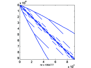
Figure 1: Sparsity pattern of the Hamiltonian matrix H in the case $N=M=10$. Every spot corresponds to a non-zero element. The dimension of the Hilbert space is $D=92\,378$ and the number of non-zero elements is $\textrm{nz}=1\,064\,777$. On average, there are $11.5$ non-zero elements per column.

5 Numerical results

After preparing the Hamiltonian in a sparse matrix form, we can use the Lanczos algorithm to compute the ground state and low lying excited states and their energies. There are some well developed packages for this purpose and our philosophy is not to reinvent the wheel. For those programming with Fortran, the ARPACK package [24] by Lehoucq et al. is a very useful aid. For those programming with MATLAB, it is enough to invoke the “eigs” command. For instance, the code

    [Evec,Eval]=eigs(H,2,’sa’)

returns the two smallest eigenvalues (the ground state energy and the first excited state energy) of H in the $2\times 2$ diagonal matrix Eval and their corresponding eigenvectors (the ground state and the first excited state) in the $D\times 2$ matrix Evec. Here we would point out that when executing “eigs”, MATLAB invokes the very ARPACK package to do the job [25].

With the ground state on hand, we can then calculate various quantities to gain some physical insights of the model. One quantity that is of primary interest is the single-particle density matrix (SPDM) associated with the many-particle ground state. In the Wannier state basis, it is defined as

$$\rho^{(1)}_{ij}=\langle G|a_{i}^{\dagger}a_{j}|G\rangle,$$ (11)

with $1\leq i,j\leq M$. All one-particle variables, e.g., the momentum distribution, are captured in the SPDM.

In general, the SPDM is hermitian, semi-positive-definite, and of trace equal to the particle number. In the present case, the SPDM is subjected to more constraints. Due to the translation and reflection invariance of the ground state [12], we have $\rho^{(1)}_{ij}=\rho^{(1)}_{i+k,j+k}$ for an arbitrary $k$ and also $\rho^{(1)}_{ij}=\rho^{(1)}_{ji}$. Therefore, the SPDM is real, symmetric, and cyclic. These good properties reduce the number of matrix elements to be computed from $M(M+1)/2$ to $[M/2]+1$, where $[\cdot]$ is the floor function.

5.1 Condensate fraction

According to the Penrose-Onsager criterion [26], a condensate is present if and only if the largest eigenvalue $\lambda_{1}$ of $\rho^{(1)}$ is macroscopic, i.e., $f_{c}=\lambda_{1}/N$ is on the order of unity and the ratio $f_{c}$ is called the condensate fraction. In the non-interacting case, all particles reside in the lowest Bloch state (a zero momentum state), and the system is in a pure condensate state with $f_{c}=1$. As the interaction is turned on, more and more particles will be kicked into higher Bloch states and the condensate is said to be depleted. In the thermodynamic limit ($M$ goes to infinity with $N/M=1$ fixed), there is a critical value [27] ($\simeq 4.65$) of $U/J$ beyond which $f_{c}$ vanishes.

To gain a picture of this phase transition, we have numerically calculated the condensate fraction as a function of the ratio $U/J$, with three different lattice sizes. The results are shown in figure 2(a). We see that as $U/J$ increases, the condensate fraction decreases monotonically. However, the finite size effect is significant. The condensate fraction is far from being vanishing in the deep Mott insulator regime ($U/J\gg 4.65$). Actually, since $\lambda_{1}\geq\left(\sum_{k}\lambda_{k}\right)/M=N/M$, $f_{c}$ has a lower bound $1/M$.

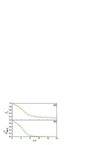
Figure 2: (Colour online) (a) Condensate fraction $f_{c}$ and (b) correlation $\rho^{(1)}_{0[M/2]}$ as functions of the ratio $U/J$. In each panel, from up to down, the size of the system is $N=M=9$, $11$, and $13$, respectively.

5.2 Off-diagonal long range order

The presence of a condensate is also associated with an off-diagonal long range order [28]. That is, a condensate is present if the off-diagonal element of the single particle density matrix $\rho^{(1)}_{ij}$ converges to a finite value as $|i-j|\rightarrow\infty$. This is consistent with the Penrose-Onsager criterion. Actually, converting into the Bloch state representation, the density matrix takes the form

$$\tilde{\rho}^{(1)}_{q_{1}q_{2}} = \langle G|b_{q_{1}}^{\dagger}b_{q_{2}}|G\rangle$$ (12)

$$= \frac{1}{M}\sum_{j_{1},j_{2}}\langle G|a_{j_{1}}^{\dagger}a_{j_{2}}|G\rangle e^{i2\pi(q_{1}j_{1}-q_{2}j_{2})/M}$$

$$= \sum\nolimits_{j}\rho^{(1)}_{0j}e^{-i2\pi q_{1}j/M}\delta_{q_{1}q_{2}}.$$

Here in the third line, we have used the cyclicity of $\rho^{(1)}$. Thus the SPDM is diagonal in the Bloch state representation. Its eigenvalues coincide with its diagonal elements, and its eigenstates (called natural orbits) coincide with the Bloch states. It can be proven that all the elements of $\rho^{(1)}$ are non-negative [12]. Therefore, the largest eigenvalue of the SPDM is just $\tilde{\rho}^{(1)}_{q_{1}q_{1}}$ with $q_{1}=0$, and is of the explicit expression

$$\lambda_{1}=\sum\nolimits_{j}\rho^{(1)}_{0j}.$$ (13)

We then see immediately that, if $\rho^{(1)}_{0j}$ decreases monotonically with $j$, $f_{c}$ and $\rho^{(1)}_{0j}$ converges to the same value in the thermodynamical limit.

Thus the phase transition can also be investigated by examining the behavior of the off-diagonal elements. In figure 2(b), we show how the element $\rho^{(1)}_{0[M/2]}$ behaves as $U/J$ varies. We choose this element because it corresponds to the correlation between two sites with the largest distance on a circle. Moreover, as $M$ tends to infinity, the distance $[M/2]$ also tends to infinity. Comparing with figure 2(a), we see that the correlation $\rho^{(1)}_{0[M/2]}$ decreases much faster than $f_{c}$, especially, in the deep Mott insulator regime, it does drop to zero.

5.3 Occupation variance

In the previous subsections, we see that both the condensate fraction and off-diagonal elements suffer from a strong finite size effect. Here, we show that the fluctuation of the occupation number on one site

$$\sigma_{i}=\sqrt{\langle G|\hat{n}_{i}^{2}|G\rangle-\langle G|\hat{n}_{i}|G\rangle^{2}}$$ (14)

is not very sensitive to the size of the lattice [29], as long as $M>>1$. In figure 3, we show $\sigma_{i}$ as a function of $U/J$ for five different lattice sizes. The difference between the curves are hardly visible. This indicates that the curve has already converged to its value in the infinite lattice limit.

This suggests that the SF-MI transition can not be tracked in any local variables. This is why we do not fix the distance between the two sites when calculating the off-diagonal element in the proceeding subsection. By the Hellmann-Feynman theorem, we have $\partial E_{G}/\partial U=\langle\partial H/\partial U\rangle=M\sigma_{i}^{2}/2$. Our numerical result for $\sigma_{i}$ suggests that the ground state energy is a smooth function of $U$.

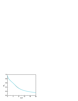
Figure 3: Variance of the occupation number $\sigma_{i}$ at an arbitrary site $i$ as a function of the ratio $U/J$ [29]. Actually five different lattice sizes, i.e., $N=M=8,9,10,11,12$, are investigated. However, the curves all collapse onto the same one.

6 Conclusion and discussion

Exact diagonalization is simple conceptually but never trivial in programming. Taking the Bose-Hubbard model as a working example, we have illustrated the architecture of numerical exact diagonalization. Some essential tricks, namely, ordering, enumerating, hashing, sorting, and searching, were explained in detail. These tricks are believed to be quite general and can be adopted in many other situations [30].

For example, we show how the idea of ordering can save computation if we want to work within the subspace $\mathcal{H}_{0}$. To impose the condition $K=0$, we had better work with $\hat{H}$ in equation (4) [14]. This time, it is the interaction part

$$\hat{H}_{int}=\frac{U}{2M}\sum_{q_{1},q_{2}}\sum_{q_{3},q_{4}}b_{q_{1}}^{\dagger}b_{q_{2}}^{\dagger}b_{q_{3}}b_{q_{4}}$$ (15)

that costs most effort. Here the condition $q_{1}+q_{2}\equiv q_{3}+q_{4}\pmod{M}$ is taken implicitly. There are exactly $M^{3}$ terms in the sum. By noting $[b_{q_{1}},b_{q_{2}}]=[b^{\dagger}_{q_{3}},b^{\dagger}_{q_{4}}]=0$, we have

$$\hat{H}_{int}=\frac{U}{2M}\sum_{q_{1}\geq q_{2}}\sum_{q_{3}\geq q_{4}}B_{q_{1}q_{2}}^{\dagger}B_{q_{3}q_{4}},$$ (16)

where $B_{q_{1}q_{2}}^{\dagger}=(2-\delta_{q_{1}q_{2}})b_{q_{1}}^{\dagger}b_{q_{2}}^{\dagger}$ is defined for $q_{1}\geq q_{2}$. We can reduce the computation further by making use of the hermicity of $\hat{H}_{int}$. We define $(q_{1}q_{2})=Mq_{1}+q_{2}$. The terms $B^{\dagger}_{q_{1}q_{2}}$ are ordered according to their tags $(q_{1}q_{2})$. We then rewrite (16) as

$$\hat{H}_{int}=\frac{U}{2M}\bigg{[}\sum_{{(q_{1}q_{2})=(q_{3}q_{4})}}B_{q_{1}q_{2}}^{\dagger}B_{q_{3}q_{4}}+\sum_{{(q_{1}q_{2})>(q_{3}q_{4})}}B_{q_{1}q_{2}}^{\dagger}B_{q_{3}q_{4}}+\sum_{{(q_{1}q_{2})<(q_{3}q_{4})}}B_{q_{1}q_{2}}^{\dagger}B_{q_{3}q_{4}}\bigg{]}.$$ (17)

The third term is hermitian conjugate to the second one. Thus in setting up the matrix corresponding to $\hat{H}_{int}$, we only need to consider the non-zero elements due to the second term, those due to the third term are then determined automatically. Overall, in the case of $N=M=10$, the number of terms need to be considered is reduced from 1000 to 180.

The readers are encouraged to convert the procedure described in this paper into codes and explore the interesting physics in the Bose-Hubbard model, which is surely far from being exhausted in the present paper. For example, we have shown how to study the condensate fraction as a function of the ratio $U/J$. On this basis, an immediately accessible problem is then how the superfluidity density varies with $U/J$. The subtle relation between condensation and superfluidity can then be investigated. For more details, see [29]. We would like to mention that the coding does not cost much effort. It takes no more than 100 lines in MATLAB, and is very efficient. For the $N=M=12$ case, it takes around 4 minutes to set up the Hamiltonian matrix and 1 minute to solve the ground state on our desktop computer. Note that the dimension is $D=1\,352\,078$. By working in the subspace $\mathcal{H}_{0}$, we have successfully performed exact diagonalization for a system as large as $N=M=13$ on our computer. Systems with larger sizes may be investigated by working in the $\mathcal{H}_{0}^{+}$ subspace. Therefore, the Bose-Hubbard model may serve as a good topic for teaching exact diagonalization in an undergraduate or graduate course of computational physics.

References

References

- [1] Lin H Q 1990 Phys. Rev. B 42 6561–7
- [2] Bloch I, Dalibard J and Zwerger W 2008 Rev. Mod. Phys. 80 885–964
- [3] Jaksch D, Bruder C, Cirac J I, Gardiner C W and Zoller P 1998 Phys. Rev. Lett. 81 3108–11
- [4] Greiner M, Mandel M O, Esslinger T, Hänsch T and Bloch I 2002 Nature (London) 415 39–44
- [5] Lanczos C 1950 J. Res. Natl. Bur. Stand. 45 255–82
- [6] Trefethen L N and Bau III D 1997 Numerical Linear Algebra (SIAM) p. 276–92
- [7] Cullum J K and Willoughby R A 1985 Lanczos Algorithms for Large Symmetric Eigenvalue Computations (Birkhauser)
- [8] Lin H Q and Gubernatis J E 1993 Comput. Phys. 7 400–7
- [9] Weiße A and Fehske F 2008 Exact Diagonalization Techniques in Computational Many-Particle Physics (Springer, Berlin Heidelberg) edited by Fehske H, Schneider R and Weiße A
- [10] Due to the periodic boundary condition, the site index is identified with .
- [11] Jafari S A 2008 Iranian J. Phys. Res. 8 No. 2 113
- [12] For , due to the connectedness of the lattice and the Perron–Frobenius theorem, the ground state must be non-degenerate and all the expansion coefficents in terms of the Fock states (7) are real and of the same sign. Therefore, we have . Since is an eigenstate of the unitary operator , we have . That is, the ground state is translationally invariant. Moreover, it is easy to show that it is also invariant under reflection. Therefore, constitutes the identity representation of the group .
- [13] The idea of defining an order in a set and so as to faciliate their enumeration is common in combinatorics; see Cameron P J 1994 Combinatorics: Topics, Techniques, Algorithms (Cambridge University Press), pp. 40–44
- [14] The same rule can be used to generate the basis vectors in the subspace . The space is spanned by which are defined as with . These states are generated one by one but only those with will be taken into . The subspace of is spanned by .
- [15] The CPU is Intel Core2, Q8200, @2.33 GHz, and the RAM is 2.5 GB.
- [16] Knuth D 1973 The Art of Computer Programming (Addison-Wesley, Reading, Mass.), Volume 3: Sorting and Searching.
- [17] Gagliano E R, Dagotto E, Moreo A and Alcaraz F C 1986 Phys. Rev. B 34 1677–82
- [18] We should mention that we use the hashing trick not in the standard way, as in [16, 17]. In our approach, we are free of the troublesome collision problem in the usual way of hashing. The coding is thus made much easier and more suitable for pedagogical use.
- [19] Physically, this can be understood as the ’s are incommensurable. Mathematically, it can be proven rigorously; see Boreico I 2008 My favorite problem: linear independence of radicals The Harvard College Mathematics Review 2 (1) 87–92
- [20] Hardy G H and Wright E M 1979 An Introduction to the Theory of Numbers (Oxford University Press, 5th Ed.) p. 381
- [21] Though on average it takes 19 trials.
- [22] Hoare C A R 1962 Comp. J. 5 10–5
- [23] Olagnon M “ORDERPACK 2.0–Unconditional, Unique, and Partial Ranking, Sorting, and Permutation,” Fortran 90 code available under http://www.fortran-2000.com/rank/.
- [24] Lehoucq R B, Sorensen D C and Yang Y “ARPACK User’s Guide: Solution to Large Scale Eigenvalue Problems with Implicitly Restarted Arnoldi Methods,” Fortran 77 code available under http://www.caam.rice.edu/software/ARPACK/.
- [25] See the Help document of Matlab.
- [26] Penrose O and Onsager L 1956 Phys. Rev. 104 576–84
- [27] Batrouni G G and Scalettar R T 1992 Phys. Rev. B 46 9051–62
- [28] Yang C N 1962 Rev. Mod. Phys. 34 694–704
- [29] Roth R and Burnett K 2003 Phys. Rev. A 68 023604
- [30] Bertsch G F and Papenbrock T 1999 Phys. Rev. Lett. 83 5412–15