Privacy-Preserving Spam Filtering

Abstract

Email is a private medium of communication, and the inherent privacy constraints form a major obstacle in developing effective spam filtering methods which require access to a large amount of email data belonging to multiple users. To mitigate this problem, we envision a privacy preserving spam filtering system, where the server is able to train and evaluate a logistic regression based spam classifier on the combined email data of all users without being able to observe any emails using primitives such as homomorphic encryption and randomization. We analyze the protocols for correctness and security, and perform experiments of a prototype system on a large scale spam filtering task.

State of the art spam filters often use character n-grams as features which result in large sparse data representation, which is not feasible to be used directly with our training and evaluation protocols. We explore various data independent dimensionality reduction which decrease the running time of the protocol making it feasible to use in practice while achieving high accuracy.

1 Introduction

Email is a private medium of communication with the message intended to be read only by the recipients. Due to the sensitive nature of the information content, there might be personal, strategic, and legal constraints against sharing and releasing email data. These constraints form formidable obstacles in many email processing applications such as spam filtering which are usually supplied by a separate service provider.

Over the years, spam has become a major problem: 75.9% all emails sent in August 2011 were spam [11]. Email users can benefit from using accurate spam filters, which could greatly reduce the loss of time and productivity due to spam email. A proficient user can directly learn a spam filtering classifier on her own private data and send it to the spam filtering provider or apply it herself, diminishing the need for a privacy preserving spam filtering system. It is, however, seen that the accuracy of spam filters based on classification models can be vastly improved by training on aggregates of data obtained from a large number of email users. This training and application of spam filters should, however, not be at the expense of user privacy, with users being required to make their emails available to the spam filtering service provider.

In this paper we propose a solution that enables users to share their private email data to train and apply spam filters while satisfying privacy constraints. We choose logistic regression as our classification model as it is widely used in spam filtering and text classification applications and is observed to achieve very high accuracy in these tasks. The training algorithm for logistic regression based on gradient ascent is more amenable to be modified to satisfy privacy constraints. The update step in the training algorithm is also particularly convenient when the training data is split among multiple parties, who can simply compute their gradient on their private email data and the server can privately aggregate these to update the model parameters. Furthermore, logistic regression is can also be easily modified to the online learning setting. In a practical spam filtering system, as the users are unlikely to relabel previously read emails as spam, the classifier needs to be learned on a continuously arriving stream of email data.

Although primarily directed at spam filtering, our solution can also be applied to any form of private text classification and in general to any binary classification setting where privacy is important, e.g., predicting the likelihood of disease based on an individual’s private medical records. Our methods also extend to batch processing scenarios.

Formally, we consider two kinds of parties: a set of users who have access to their private emails and server who is interested in training a spam classification model over the complete email data. The users can communicate with the server but not with each other as this is typically the case in an email service. The primary privacy constraint is that the server should not be able to observe the emails belonging to any of the users and similarly, any user should not be able to observe emails belonging to any other user. The secondary privacy constraint is that the users should not be able to observe the parameters of the classification model learned by the server. While the motivation behind the former privacy constraint is more obvious, the server might want to keep the classification model private if it was privately trained over large quantities of training data pooled from a large number of users and if the server is interested in offering a restricted pay per use spam filtering service. We present protocols to train and evaluate logistic regression models while maintaining these privacy constraints.

Our privacy preserving protocol falls into the broad class of secure multiparty computation (SMC) algorithms [15]. In the SMC framework, multiple parties desire to compute a function that combines their individual inputs. The privacy constraint is that no party should learn anything about inputs belonging to any other party besides what can be inferred from the value of the function. We construct our protocol using a cryptosystem satisfying homomorphic encryption [9], in which operations on encrypted data correspond to operations on the original unencrypted data (Section 3.2). We further augment our protocol with additive and multiplicative randomization, and present an information theoretic analysis of the security of the protocol.

The benefit of training and evaluating a spam filtering classifier privately comes with a substantial overhead of computation and data transmission costs. We find that these costs are linear in the number of training data instances and the data dimensionality. As the size of our character four-gram feature representation of the text data is extremely large (e.g., one million features), application of our protocol on a typical email dataset is prohibitively expensive. Towards this, we apply suitable data dimensionality reduction techniques to make the training protocol computationally usable in practical settings. As the same dimensionality reduction is has to be applied by all the parties to their private data, we require that the techniques used are data independent and do not require to be computed separately. We present extensive evaluation of our protocol on a large scale email dataset from the CEAS 2008 spam filtering challenge. With data independent dimensionality reduction such as locality sensitive hashing, multinomial sampling, and hash space reduction, we demonstrate that our protocol is able to achieve state of the art performance in a feasible amount of running time.

To summarize, our main contributions are:

• Protocols for training and evaluating the logistic regression based spam filtering classifier with online updates from while preserving the private email data belonging to multiple parties.

• Analysis of the protocols for security and efficiency.

• Dimensionality reduction for making the protocol feasible to be used in a practical spam filtering task.

• Experiments with the privacy preserving training and evaluation protocols over a large scale spam dataset: trade off between running time and accuracy.

2 Related Work

Email spam filtering is a well established area of research. The accuracy of the best systems in the 2007 CEAS spam filtering competition was better than 0.9999 [3]. Our implementation is an online logistic regression classifier implementation inspired by [5] which on application to binary character four-gram features was shown to have near state of the art accuracy [3].

The application of privacy preserving techniques to large scale real world problems of practical importance, such as spam filtering, is an emerging area of research. Li, et al. [6] present a distributed framework for privacy aware spam filtering. Their method is based on applying a one-way fingerprinting transformation [1] to the message text and comparing two emails using a Hamming distance metric and does not involve statistical learning. Additionally, this method also requires that the spam emails belonging to all users should be revealed which does not match our privacy criteria. We consider all emails to be private as the nature of the spam emails a user receives might be correlated to the user’s online and offline activities.

There has also been recent work on constructing privacy preserving protocols for general data mining tasks including decision trees [12], clustering [7], naive Bayes [13], and support vector machines [14]. To the best of our knowledge, this paper is the first to describe a practical privacy-preserving framework using a logistic regression classifier applied to a real world spam filtering task.

3 Preliminaries

3.1 Classification Model: Logistic Regression in the Batch and Online Settings

The training dataset consisting of $n$ documents classified by the user as spam or ham (i.e., not spam) are represented as the labeled data instances $(x,y)=\{(x_{1},y_{1}),\ldots,(x_{n},y_{n})\}$ where $x_{i}\in\mathbb{R}^{d}$ and $y_{i}\in\{-1,1\}$. In the batch learning setting, we assume that the complete dataset is available at a given time. In the logistic regression classification algorithm, we model the class probabilities by a sigmoid function

$$P(y_{i}=1|x_{i},w)=\frac{1}{1+e^{-y_{i}w^{T}x_{i}}}.$$

We denote the log-likelihood for the weight vector $w$ computed over the data instances $(x,y)$ by $L(w,x,y)$. Assuming the data instances to be i.i.d., the data log-likelihood $L(w,x,y)$ is equal to

$$L(w,x,y)=\log\prod_{i}\frac{1}{1+e^{-y_{i}w^{T}x_{i}}}=-\sum_{i}\log[1+e^{-y_{i}w^{T}x_{i}}].$$

We maximize the data log-likelihood $L(w,x,y)$ using gradient ascent to obtain the classifier with the optimal weight vector $w^{*}$. Starting with a uniformly initialized vector $w_{(0)}$, in the $t^{\rm th}$ iteration, we update $w_{(t)}$ as

$$w_{(t+1)}=w_{(t)}+\eta\nabla L(w_{(t)},x,y)=w_{(t)}+\eta\sum_{i}\frac{y_{i}x_{i}^{T}}{1+e^{y_{i}w_{(t)}^{T}x_{i}}},$$ (1)

where $\eta$ is the pre-defined step size. We terminate the procedure on convergence between consecutive values of $w_{(t)}$.

In the online learning setting, the data instances are obtained incrementally rather than being completely available at a given instance of time. In this case, we start with a model with the uniformly random weight vector $w_{(0)}$. A model $w_{(t)}$ learned using the first $t$ instances, is updated after observing a small block of $k$ instances. with the gradient of the log-likelihood computed over that block.

3.2 Homomorphic Encryption

In a homomorphic cryptosystem, operations performed on encrypted data (ciphertext) map to the corresponding operations performed on the original unencrypted data (plaintext). If $+$ and $\cdot$ are two operators and $x$ and $y$ are two plaintexts, a homomorphic encryption function $E$ satisfies

$$E[x]\cdot E[y]=E[x+y].$$

This allows one party to encrypt the data using a homomorphic encryption scheme and another party to perform operations without being able to observe the plaintext data. This property forms the fundamental building block of our privacy preserving protocol.

In this work we use the additively homomorphic Paillier cryptosystem [9] which also satisfies semantic security. The Paillier key generation algorithm produces a pair of $b$-bit numbers $(N,g)$ constituting the public key corresponding to the encryption function $E:\mathbb{Z}_{N}\mapsto\mathbb{Z}_{N^{2}}$ and another pair of $b$-bit numbers $(\lambda,\mu)$ constituting the private key corresponding to the decryption function $D:\mathbb{Z}_{N^{2}}\mapsto\mathbb{Z}_{N}$.

Given a plaintext $x\in\mathbb{Z}_{N}$, the encrypted text is given by:

$$E[x]=g^{x}r^{n}\mod N^{2},$$

where $r$ is a random number sampled uniformly from $\mathbb{Z}_{N}$. Using a different value of the random number $r$ provides semantic security, i.e., two different encryptions of a number $x$ say, $E[x;r_{1}]$ and $E[x;r_{2}]$ will have different values but decrypting each of them will result in the same number $x$. It can be easily verified that the above encryption function satisfies the following properties:

1. For any two ciphertexts $E[x]$ and $E[y]$,

   $$E[x]~{}E[y]=E[x+y\mod N^{2}].$$

2. And as a corollary, for any ciphertext $E[x]$ and plaintext $y$,

   $$E[x]^{y}=E[x~{}y\mod N^{2}].$$

Extending the Encryption Function to Real Numbers

Paillier encryption as most other cryptosystems is defined over the finite field $\mathbb{Z}_{N}=\{0,\ldots,N-1\}$. However, in our protocol we need to encrypt real numbers, such as the training data and model parameters. We make the following modifications to the encryption function to support this.

1. Real numbers are converted to a fixed precision floating point representation. For a large constant $C$, a real number $x$ is represented as $\lfloor Cx\rfloor=\bar{x}$.

   $$E[\bar{x}]=E[\lfloor Cx\rfloor],\quad D[E[\bar{x}]]=E[\lfloor Cx\rfloor]/C=x.$$

2. The encryption of a negative integer is represented by the encryption of its modular additive inverse. If $-x$ is a negative integer,

   $$E[-x]=E[N-x].$$

3. Exponentiation of an encrypted number by a negative integer is represented as the exponentiation of the multiplicative inverse of the encryption in the $\mathbb{Z}_{N^{2}}$ field, by the corresponding positive integer. We represent the exponentiation the ciphertext $E[x]$ by a negative integer $-y$ as

   $$E[x]^{-y}=E[x^{-1}\mod N^{2}]^{y}.$$

Representing real numbers by a fixed precision number introduces a small error due to the truncation which is directly proportional to the value of $C$. This representation also reduces the domain of the encryption function from $\{0,\ldots,N-1\}$ to $\{0,\ldots,\lfloor\frac{N-1}{C}\rfloor\}$. We need to ensure that the result of homomorphic operations on encrypted functions do not overflow the range, so we need to increase the bit-size $b$ of the encryption keys proportionally with $C$. As the computational cost of the encryption operations is also proportional to $b$, this creates a trade-off between accuracy and computation cost.

The representation of negative integers on the other hand does not introduce any error but further halves the domain of the encryption function from $\{0,\ldots,\lfloor\frac{N-1}{C}\rfloor\}$ to $\{0,\ldots,\lfloor\frac{N-1}{2C}\rfloor\}$ which we denote by $\mathcal{D}$.

4 Privacy Preserving Classifier
Training and Evaluation

4.1 Data Setup and Privacy Conditions

We define the party “Bob” who is interested in training a logistic regression classifier with weight vector $w\in\mathbb{R}^{d}$. In the online learning setting, multiple users interact with Bob at one time using their private training data as input. As all these parties play the same role in their interactions with Bob in one update step, we represent them by a generic user “Alice”. Later on we see how Bob privately aggregates the encrypted gradients provided by individual parties.

Alice has a sequence of labeled training data instances $(x,y)=\{(x_{1},y_{1}),\ldots,(x_{n},y_{n})\}$. Bob is interested in training a logistic regression classifier with weight vector $w\in\mathbb{R}^{d}$ over $(x,y)$ as discussed in Section 3.1. The privacy constraint implies that Alice should not be able to observe $w$ and Bob should not be able to observe $(x_{i},y_{i})$. The parties are assumed to be semi-malicious, i.e., they correctly execute the steps of the protocol and do not attempt to cheat by using fraudulent data as input in order to extract additional information about the other parties. The parties are assumed to be curious, i.e., they keep a transcript of all intermediate results and can use that to gain as much information as possible.

4.2 Private Training Protocol

Bob generates a public and private key pair for a $b$-bit Paillier cryptosystem and provides the public key to Alice. In this cryptosystem, Bob is able to perform both encryption and decryption operations while Alice can perform only encryption.

As mentioned before, we use the homomorphic properties of Paillier encryption to allow the parties to perform computations using private data. The update rule requires Bob to compute the gradient of the data log-likelihood function $\nabla L(w_{(t)},x,y)$ which involves exponentiation and division and cannot be done using only homomorphic additions and multiplications. We supplement the homomorphic operations with Bob performing those operations on multiplicative shares to maintain the privacy constraints. As mentioned in Section 3.2, the domain of the encryption function is $\mathcal{D}=\{0,\ldots,\lfloor\frac{N-1}{2C}\rfloor\}$. We sample the randomizations uniformly from this set.

Bob initiates the protocol with a uniform $w_{(0)}$ and the gradient update step $\eta$ is publicly known. We describe the $t^{\rm th}$ iteration of the protocol below. 

Input: Alice has $(x,y)$ and the encryption key,
Bob has $w_{(t)}$ and both encryption and decryption keys.
Output: Bob has $w_{(t+1)}$.

1. Bob encrypts $w_{(t)}$ and transfers $E[w_{(t)}]$ to Alice.

2. For each training instance $x_{i}$, $i=1,\ldots,n$, Alice computes

   $$\prod_{j=1}^{d}E[w_{(t)j}]^{y_{i}x_{ij}}=E\left[\sum_{j=1}^{d}y_{i}w_{(t)j}x_{ij}\right]=E\left[y_{i}w_{(t)}^{T}x_{i}\right].$$

3. Alice samples $n$ numbers $r_{1},\ldots,r_{n}$ uniformly from $\mathbb{Z}_{N}=\{1,\ldots,N-1\}$ and computes

   $$E\left[y_{i}w_{(t)}^{T}x_{i}\right]\cdot E[-r_{i}]=E\left[y_{i}w_{(t)}^{T}x_{i}-r_{i}\right].$$

   Alice transfers $E\left[y_{i}w_{(t)}^{T}x_{i}-r_{i}\right]$ to Bob.

4. Bob decrypts this to obtain $y_{i}w_{(t)}^{T}x_{i}-r_{i}$. In this way, Alice and Bob have additive shares of the inner products $y_{i}w_{(t)}^{T}x_{i}$.

5. Bob exponentiates and encrypts his shares of the inner products. He transfers $E\left[e^{y_{i}w_{(t)}^{T}x_{i}-r_{i}}\right]$ to Alice.

6. Alice homomorphically multiplies the quantities she obtained from Bob by the exponentiations of her corresponding random shares to obtain the encryption of the exponentiations of the inner products.

   $$E\left[e^{y_{i}w_{(t)}^{T}x_{i}-r_{i}}\right]^{e^{r_{i}}}=E\left[e^{y_{i}w_{(t)}^{T}x_{i}}\right].$$

   Alice homomorphically adds $E[1]$ to these quantities to obtain $E\left[1+e^{y_{i}w_{(t)}^{T}x_{i}}\right]$.

7. Alice samples $n$ numbers $q_{1},\ldots,q_{n}$ from $\mathcal{D}$ using a bounded Power law distribution. She then homomorphically computes

   $$E\left[1+e^{y_{i}w_{(t)}^{T}x_{i}}\right]^{q_{i}}=E\left[q_{i}\left(1+e^{y_{i}w_{(t)}^{T}x_{i}}\right)\right].$$

   She transfers these quantities to Bob.

8. Bob decrypts these quantities and computes the reciprocal $\frac{1}{q_{i}\left(1+e^{y_{i}w_{(t)}^{T}x_{i}}\right)}$. He then encrypts the reciprocals and sends them to Alice.

9. Alice homomorphically multiplies $q_{i}$ with the encrypted reciprocals to cancel out her multiplicative share.

   $$E\left[\frac{1}{q_{i}\left(1+e^{y_{i}w_{(t)}^{T}x_{i}}\right)}\right]^{q_{i}}=E\left[\frac{1}{1+e^{y_{i}w_{(t)}^{T}x_{i}}}\right].$$

10. Alice then homomorphically multiplies the encrypted reciprocal by each component of $y_{i}x_{i}^{T}$ to obtain the encrypted $d$-dimensional vector

    $$E\left[\frac{1}{1+e^{y_{i}w_{(t)}^{T}x_{i}}}\right]^{y_{i}x_{i}^{T}}=E\left[\frac{y_{i}x_{i}^{T}}{1+e^{y_{i}w_{(t)}^{T}x_{i}}}\right].$$

    She homomorphically adds each encrypted component to obtain

    $$\prod_{i}E\left[\frac{y_{i}x_{i}^{T}}{1+e^{y_{i}w_{(t)}^{T}x_{i}}}\right]=E\left[\sum_{i}\frac{y_{i}x_{i}^{T}}{1+e^{y_{i}w_{(t)}^{T}x_{i}}}\right].$$

    This is the encrypted gradient vector $E\left[\nabla L(w_{(t)},x,y)\right]$.

11. Alice homomorphically updates the encrypted weight vector she obtained in Step 1 with the gradient.

    $$E[w_{(t+1)}] =E[w_{(t)}]~{}E\left[\nabla L(w_{(t)},x,y)\right]^{\eta}$$

    $$=E\left[w_{(t)}+\eta\nabla L(w_{(t)},x,y)\right].$$

12. Alice then sends the updated weight vector $E[w_{(t+1)}]$ to Bob who then decrypts it to obtain his output.

In this way, Bob is able to update his weight vector using Alice’s data while maintaining the privacy constraints. In the batch setting, Alice and Bob repeat Steps 2 to 11 to perform the iterative gradient descent. Bob can check for convergence in the value of $w$ between iterations by performing Step 12. In the online setting, Alice and Bob execute the protocol only once with using Alice using a typically small block of $k$ data instances as input.

Extensions to the Training Protocol

1. Training on private data horizontally split across multiple parties.

   In the online setting we do not make any assumption about which data holding party is participating in the protocol. Just as Alice uses her data to update $w$ privately, other parties can then use their data to perform the online update using the same protocol.

   In the batch setting, multiple parties can execute one iteration of the protocol individually with Bob to compute the encrypted gradient on their own data. Finally, Bob can receive the encrypted gradients from all the parties and update the weight vector as follows.

   $$w_{(t+1)}=w_{(t)}+\eta\sum_{k}\nabla L(w_{(t)},x^{k},y^{k}),$$

   where $(x^{1},y^{1}),\ldots,(x^{K},y^{K})$ are the individual datasets belonging to $K$ parties.

2. Training a regularized classifier.

   The protocol can easily be extended to introduce $\ell_{2}$ regularization, which is a commonly used method to prevent over-fitting. In this case the update rule becomes

   $$w_{(t+1)}=w_{(t)}+\eta\nabla L(w_{(t)},x,y)+2\lambda w_{(t)},$$

   where $\lambda$ is the regularization parameter.

   This can be accommodated by Alice homomorphically adding the term $2\lambda w_{(t)}$ to the gradient in Step 11.

   $$E[w_{(t+1)}] =E[w_{(t)}]^{1+2\lambda}~{}E\left[\nabla L(w_{(t)},x,y)\right]^{\eta}$$

   $$=E\left[(1+2\lambda)w_{(t)}+\eta\nabla L(w_{(t)},x,y)\right].$$

   In order to identify the appropriate value of $\lambda$ to use, Alice and Bob can perform $m$-fold cross-validation by repeatedly executing the private training and evaluation protocols over different subsets of data belonging to Alice.

4.3 Private Evaluation Protocol

Another party “Carol” having one test data instance $x^{\prime}\in\mathbb{R}^{d}$ is interested in applying the classification model with weight vector $w$ belonging to Bob. Here, the privacy constraint require that Bob should not be able to observe $x^{\prime}$ and Carol should not be able to observe $w$. Similar to the training protocol, Bob generates a public and private key pair for a $b$-bit Paillier cryptosystem and provides the public key to Carol.

In order to label the data instance as $y^{\prime}=1$, Carol needs to check if $P(y^{\prime}=1|x^{\prime},w)=\frac{1}{1+e^{-w^{T}x^{\prime}}}>\frac{1}{2}$ and vice-versa for $y^{\prime}=-1$. This is equivalent to checking if $w^{T}x^{\prime}>0$. We develop the following protocol towards this purpose. 

Input: Bob has $w$ and generates a public-private key pair.
Carol has $x^{\prime}$ and Bob’s public key.
Output: Carol knows if $w^{T}x^{\prime}>0$.

1. Bob encrypts $w$ and transfers $E[w]$ to Carol.

2. Carol homomorphically computes the encrypted inner product.

   $$\prod_{j=1}^{d}E[w]^{x_{j}^{\prime}}=E\left[\sum_{j=1}^{d}w_{j}x_{j}^{\prime}\right]=E\left[w^{T}x^{\prime}\right].$$

3. Carol generates a random number $r$ and sends $E\left[w^{T}x^{\prime}\right]-r$ to Bob.

4. Bob decrypts it to obtain his additive share $w^{T}x^{\prime}-r$. Let us denote it by $-s$, so that $r-s=w^{T}x^{\prime}$.

5. Bob and Carol execute a variant of the secure millionaire protocol [15] to with inputs $r$ and $s$ and both learn whether $r>s$.
   If $r>s$, Carol concludes $w^{T}x^{\prime}>0$ and if $r<s$, she concludes $w^{T}x^{\prime}<0$.

In this way, Carol and Bob are able to perform the classification operation while maintaining the privacy constraints. If Bob has to repeatedly execute the same protocol, he can pre-compute $E[w]$ to be used in Step 1.

5 Analysis

5.1 Correctness

The private training protocol does not alter any of the computations of the original training algorithm and therefore results in the same output. The additive randomization $r_{i}$ introduced in Step 3 is removed in Step 6 leaving the results unchanged. Similarly, the multiplicative randomization $q_{i}$ introduced in Step 7 is removed in Step 9.

As discussed in Section 3.2, the only source of error is the truncation of less significant digits in the finite precision representation of real numbers. In practice, we observe that the error in computing the weight vector $w$ is negligibly small and does not result in any loss of accuracy.

5.2 Security

The principal requirement of a valid secure multiparty computation (SMC) protocol is that any party must not learn anything about the input data provided by the other parties apart from what can be inferred from the result of the computation itself. As we mentioned earlier, we assume that the parties are semi-malicious. From this perspective, it can be seen that the private training protocol (Section 4.2) is demonstrably secure.  

Alice/Carol: In the private training protocol, Alice can only observe encrypted inputs from Bob and hence she does not learn anything about the weight vector used by Bob. In the private classifier evaluation protocol, the party Carol with the test email only receives the final outcome of the classifier in plaintext. Thus, the only additional information available to her is the output of the classifier itself, which being the output is permissible under the privacy criteria of the problem. 

Bob: In the training stage, Bob receives unencrypted data from Alice in Steps 3, 8 and 12.

• Step 3: Bob receives $y_{i}w^{T}_{(t)}x_{i}-r_{i}$. Let us denote this quantity by $v$ and $yw^{T}x$ by $z$, giving us $v=z-r_{i}$. Since $r_{i}$ is drawn from a uniform distribution over the entire finite field $\mathbb{Z}_{N}$, for any $v$ and for every value of $z$ there exists a unique value of $r_{i}$ such that $v=z-r_{i}$. Thus, $P_{z}(z|v)\propto P_{z}(z)P_{r}(z-v)=P_{z}(z)$. The conditional entropy $H(z|v)=H(z)$, i.e., Bob receives no information from the operation.

• Step 8: A similar argument can be made for this step. Here Bob receives $v=qz$, where $z=1+e^{y_{i}w^{T}_{(t)}x_{i}}$. It can be shown that for any value $v$ that Bob receives, $P_{z}(z|v)\propto\frac{P_{z}(z)P_{q}(v/z)}{z}$. Since $q$ is drawn from a power law distribution, i.e. $P_{q}(q)\propto 1/q$, for all $v<|\mathcal{D}|$, $P_{z}(z|v)=P_{z}(z)$. Once again, the conditional entropy $H(z|v)=H(z)$, i.e., Bob receives no information from the operation.

• Step 12: The information Bob receives in this step is the updated weight vector, which is the result of the computation that Bob is permitted to receive by the basic premise of the SMC protocol.

Information Revealed by the Output

We assume that all the parties agree with Bob receiving the updated classifier at the end of the training protocol, this forms the premise behind their participation in the protocol to start with. If the parties use the modified training protocol which results in a differentially private classifier, no information about the data can be gained from the output classifier. In case the parties use the original training protocol, the output classifier does reveal information about the input data, which we quantify and present ways to minimize in the following analysis.

At the end of Step 12 in each iteration, Bob receives the update weight vector $w_{t+1}=w_{t}+\eta\nabla L(w_{(t)},x,y)$. As he also has the previous weight vector $w_{t}$, he effectively observes the gradient $\nabla L(w_{(t)},x,y)=\sum_{i}y_{i}x^{T}_{i}\left(1+e^{y_{i}w^{T}_{(t)}x_{i}}\right)^{-1}$.

In the online setting, we normally use one training data instance at a time to update the classifier. If Alice participates in the training protocol using only one document $(x_{1},y_{1})$, the gradient observed by Bob will be $y_{1}x_{1}\left(1+e^{y_{1}w^{T}_{(t)}x_{i}}\right)^{-1}$, which is simply a scaling of the data vector $y_{1}x_{1}$. As Bob knows $w_{(t)}$ he effectively knows $y_{1}x_{1}$. In particular, if $x_{1}$ is a vector of non-negative counts as is the case for n-grams, the knowledge of $y_{1}x_{1}$ is equivalent to knowing $x_{1}$. Although the protocol itself is secure, the output reveals Alice’s data completely.

Alice can prevent this by updating the classifier using blocks of $K$ document vectors $(x,y)$ at a time. The protocol ensures that for each block of $K$ vectors Bob only receives the gradient computed over them

$$\nabla L(w_{(t)},x,y) =\sum_{i=1}^{K}y_{i}x^{T}_{i}\left(1+e^{y_{i}w^{T}_{(t)}x_{i}}\right)^{-1}$$

$$=\sum_{i=1}^{K}g(w_{(t)},x_{i},y_{i})x_{i},$$

where $g(w_{(t)},x_{i},y_{i})$ is a scalar function of the data instance such that $g(w_{(t)},x_{i},y_{i})x_{i}$ has a one-to-one mapping to $x_{i}$. Assuming that all data vectors $x_{i}$ are i.i.d., using Jensen’s inequality, we can show that the conditional entropy

$$H\left[x_{i}|\nabla L(w_{(t)},x,y)\right]\leq\frac{K-1}{K}H[x_{i}]+\log(K).$$ (2)

In other words, while Bob gains some information about the data belonging to Alice, the amount of this information is inversely proportional to the block size. In the online learning setting, choosing a large block size decreases the accuracy of the classifier. Therefore, the choice of the block size effectively becomes a parameter that Alice can control to trade off giving away some information about her data with the accuracy of the classifier. In Section 6.2, we empirically analyze the performance of the classifier for varying batch sizes. We observe that in practice, the accuracy of the classifier is not reduced even after choosing substantially large batches of 1000 documents, which would hardly cause any loss of information as given by Equation 2.

5.3 Complexity

We analyze the encryption/decryption and the data transmission costs for a single execution of the protocol as these consume a vast majority of the time.

There are 6 steps of the protocol where encryption or decryption operations are carried out.

1. In Step 1, Bob encrypts the $d$-dimensional vector $w_{(t)}$.

2. In Step 3, Alice encrypts the $n$ random numbers $r_{i}$.

3. In Step 4, Bob decrypts the $n$ inner products obtained from Alice.

4. In Step 5, Bob encrypts the exponentiation of the $n$ inner products.

5. In Step 8, Bob decrypts, takes a reciprocal, and encrypts the $n$ multiplicatively scaled quantities.

6. In Step 12, Bob decrypts the $d$ dimensional updated weight vector obtained from Alice.

Total: $3n+2d$ encryptions and decryptions. 

Similarly, there are 6 steps of the protocol where Alice and Bob transfer data to each other.

1. In Step 1, Bob transfers the $d$-dimensional vector $w_{(t)}$ to Alice.

2. In Step 3, Alice transfers $n$ randomized innner products to Bob.

3. In Step 5, Bob transfers the $n$ encrypted exponentials to Alice.

4. In Step 7, Alice transfers $n$ scaled quantities to Bob.

5. In Step 8, Bob transfers the $n$ encrypted reciprocals to Alice.

6. In Step 11, Alice transfers the $d$ dimensional encrypted updated weight vector to Bob.

Total: Transmitting $4n+2d$ elements. 

The speed of performing the encryption and decryption operations depends directly on the size of the key of the cryptosystem. Similarly, when we are transfering encrypted data, the size of an individual element also depends on the size of the encryption key. As the security of the encryption function is largely determined by the size of the encryption key, this reflects a direct trade-off between security and efficiency.

6 Experiments

We provide an experimental evaluation of our approach for the task of email spam filtering. The privacy preserving training protocol requires a substantially larger running time as compared to the non-private algorithm. In this section, we analyze the training protocol for running time and accuracy. As the execution of the protocol on the original dataset requires an infeasible amount of time, we see how data independent dimensionality reduction can be used to effectively reduce the running time while still achieving comparable accuracy.

As it is conventional in spam filtering research, we report AUC scores. It is considered to be a more appropriate metric for this task as compared to other metrics such as classification accuracy or F-measure because it averages the performance of the classifier in different precision-recall points which correspond to different thresholds on the prediction confidence of the classifier. The AUC score of a random classifier is 0.5 and that for the perfect classifier is 1. We compared AUC performance of the classifier given by the privacy preserving training protocol with the non-private training algorithm and in all cases the numbers were identical up to the five significant digits. Therefore, the error due to the finite precision representation mentioned in Section 5.1 is negligible for practical purposes.

Table 1: Email spam dataset summary.

Section	Spam	Non-spam	Total
Training	2466 (82%)	534 (18%)	3000
Testing	2383 (79%)	617 (21%)	3000

6.1 Email Spam Dataset

We used the public spam email corpus from the CEAS 2008 spam filtering challenge. For generality, we refer to emails as documents. Performance of various algorithms on this dataset is reported in [10]. The dataset consists of 3,067 training and 206,207 testing documents manually labeled as spam or ham (i.e., not spam). To simplify the benchmark calculations, we used the first 3000 documents from each set (Table 1). Accuracy of the baseline majority classifier which labels all documents as spam is 0.79433.

6.2 Spam Filter Implementation

Our classification approach is based on online logistic regression [5], as described in Section 3.1. The features are overlapping character four-grams which are extracted from the documents by a sliding window of four characters. The feature are binary indicating the presence or absence of the given four-gram. The documents are in ASCII or UTF-8 encoding which represents each character in 8 bits, therefore the space of possible four-gram features is $2^{32}$. Following the previous work, we used modulo $10^{6}$ to reduce the four-gram feature space to one million features and only the first 35 KB of the documents is used to compute the features. For all experiments, we use a step size of $\eta=0.001$ and no regularization or noise required for differential privacy is used.

Table 2: Running time comparison of online training of logistic regression (LR) and the privacy preserving logistic regression (PPLR) for one document.

Feature Count	LR	PPLR
Original: $10^{6}$	0.5 s	1.14 hours
Reduced: $10^{4}$	5 ms	41 s

Table 3: Running time of privacy preserving logistic regression for one document of $10^{4}$ features with different encryption key sizes.

Encryption Key Size	Time
256 bit	41 s
1024 bit	2013 s

Table 4: Time requirement for steps of the protocol for random matrices of the dimensions shown (documents $\times$ features).

Steps	Time (s) - 200$\times$20	Time (s) - 200$\times$100
1	0.06	0.31
2, 3	2.59	10.14
4, 5	0.82	0.73
6, 7	0.46	0.41
8	0.84	0.73
9, 10	1.81	8.33
11	0.05	0.18
Total	6.61	20.81

6.3 Protocol Implementation

We created a prototype implementation of the protocol in C++ and used the variable precision arithmetic libraries provided by OpenSSL [8] to implement the Paillier cryptosystem. We used the GSL libraries [4] for matrix operations. We performed the experiments on a 3.2 GHz Intel Pentium 4 machine with 2 GB RAM and running 64-bit Ubuntu.

The original dataset has $10^{6}$ features as described in Section 6.2. Similar to the complexity analysis of the training protocol (Section 5.1), we observed that time required for the training protocol is linear in number of documents and number of features.

Table 2 compares the time required to train a logistic regression classifier with and without the privacy preserving protocol using 256-bit encryption for one document. It can be seen that the protocol is slower than non-private version by a factor of $10^{4}$ mainly due to the encryption in each step of the protocol. Also, we observe that the running time is drastically reduced with the dimensionality reduction. While the execution time for the training protocol over the original feature space would be infeasible for most applications, the execution time for the reduced feature space is seen to be usable in spam filtering applications. This motivated us to consider various dimensionality reduction schemes which we discuss in Section 6.4.

To further analyze the behavior of various steps of the protocol, in Table 4 we report the running time of individual steps of the protocol outlined in Section 4.2 on two test datasets of random vectors. It can be observed that encryption is the main bottle neck among the other operations in the protocol. We report the Paillier cryptosystem with 256-bit keys in the following experiments. As shown in Table 3, using the more secure 1024-bit encryption keys, resulted in a slowdown by a factor of about 50 as compared to using 256-bit encryption keys. This is a constant factor which can be applied to all our timing results if the stronger level of security provided by 1024-bit keys is desired.

Using a pre-computed value of the encrypted weight vector $E[w]$, the private evaluation protocol took 210.956 seconds for one document using $10^{6}$ features and 2.059 seconds for one document using $10^{4}$ features which again highlights the necessity for dimensionality reduction to make the private computation feasible.

6.4 Dimensionality Reduction

Since the time requirement of the privacy preserving protocol varies linearly with the data dimensionality, we can improve it by dimensionality reduction principally because data with fewer number of features will require fewer encryptions and decryptions. On the other hand, reducing the dimensionality of the features, particularly for sparse features such as $n$-gram counts, can have an effect on the classification performance. We study this behavior by experimenting with six different dimensionality reduction techniques, and compared the running time and AUC of the classifier learned by the training protocol.

We consider PCA which is a data-dependent dimensionality reduction technique and five other ones which are data independent. The latter techniques are much more in our setting as they can be used by multiple parties on their individual documents without violating privacy.

Table 5: Performance of PCA for dimensionality reduction.

Dimension	Time (s)	AUC
5	18	0.96159
10	37	0.99798
50	242	0.99944
100	599	0.99967
300	5949	0.99981

Table 6: Time and space requirement for dimensionality reduction methods for reduction from $10^{6}$ to $10^{4}$ features.

Method	Time (s)	Space (GB)
PCA	7 $\times 10^{6}$	41
LSH	50 $\times 10^{3}$	40
Hash Space	41	–
Document Frequency	1	–
Sample Uniform	2	–
Sample Multinomial	490	–

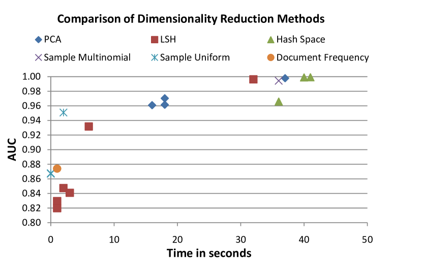
Figure 1: Time comparison for the dimensionality reduction approaches reduced from $10^{6}$ to $10^{4}$ dimensions.

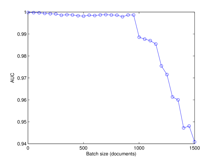
Figure 2: Performance of one iteration of logistic regression training on 300 dimensional PCA feature vectors with different batch sizes.

1. Principal Component Analysis (PCA): PCA is perhaps the most commonly used dimensionality reduction technique which computes the lower dimensional projection of the data based on the most dominant eigenvectors of covariance matrix of the original data. Since we only compute a small number of eigenvectors, PCA is found to be efficient for our sparse binary dataset. Table 5 summarizes the running time and the AUC of the classifier trained on the reduced dimension data. While the performance of PCA is excellent, it has the following disadvantages, motivating us to look at other techniques.

   1. When training in a multiparty setting, all the parties are required to use a common feature representation. Among the methods we considered, only PCA computes a projection matrix which is data dependent. This projection matrix cannot be computed over the private training data because it reveals information about the data.

   2. For many classification tasks, reduction to an extremely small subspace hurts the performance much more significantly than in our case. Furthermore, computing PCA with high dimensional data is not efficient and we are interested in efficient and scalable dimensionality reduction techniques.

2. Locality Sensitive Hashing (LSH): In LSH [2], we choose $k$ random hyperplanes in the original $d$ dimensional space which represent each dimension in the target space. The reduced dimensions are binary and indicate the side of the hyperplane on which the original point lies.

3. Hash Space Reduction: As mentioned in Section 6.2, we reduce the original feature space to modulo $10^{6}$. We experimented with different sizes of this hash space.

4. Document Frequency Based Pruning: We select features which occur in at least $k$ documents. This is a common approach in removing rarely-occurring features, although some of those feature could be discriminative especially in a spam filtering task.

5. Uniform Sampling: In this approach, we draw from the uniform distribution until desired number of unique features are selected.

6. Multinomial Sampling: This approach is similar to the uniform sampling approach except that we first fit a multinomial distribution based on the document frequency of the features and then draw from this distribution. This causes the sampling to be biased toward features with higher variance which are often the more informative features.

We ran each of these algorithms on 6000 documents of $10^{6}$ dimensions. Table 6 summarizes the time and space requirement of each algorithm for reducing dimensions to $10^{4}$. We trained the logistic regression classifier on 3000 training documents with various reduced dimensions and measured the running time and AUC of the learned classifier on the 3000 test documents. The results are shown in Figure 1. We observe that the data independent dimensionality reduction techniques such as LSH, multinomial sampling, and hash space reduction achieve close to perfect AUC.

Classifier Performance for Varying Batch Size

As we discussed in Section 5.2, another important requirement of our protocol is to train in batches of documents rather than training on one document at a time. We have shown that the extra information gained by Bob about any party’s data decreases with the increasing batch size. On the other hand, increasing the batch size causes the optimization procedure of the training algorithm to have fewer chances of correcting itself in a single pass over the entire training dataset. In Figure 2, we see that the trade-off in AUC is negligible even with batch sizes of around 1000 documents.

6.5 Parallel Processing

An alternative approach to address the performance issue is parallelization. We experimented with a multi-threaded implementation of the algorithm. On average, we observed 6.3% speed improvement on a single core machine. We expect the improvement to be more significant on a multi-core architecture. A similar scheme can be used to parallelize the protocol across a cluster of machines, such as in a MapReduce framework. In both of these cases, the accuracy of the online algorithms will decrease slightly as the number of threads or machines increase because the gradient $\nabla L(w_{(t)},x,y)$ computed in each of the parallel processes is based on an older value of the weight vector $w_{(t)}$.

A more promising approach which does not impact the accuracy is encrypting vectors in parallel. In the present implementation of the protocol, we encrypt vectors serially and the procedure used for the individual elements is identical. We can potentially reduce the encryption time of a feature vector substantially by using a parallel processing infrastructure such as GPUs. We leave the experiments with such an implementation for future work.

7 Conclusion

We developed protocols for training and evaluating a logistic regression based spam filtering classifier over emails belonging to multiple parties while preserving the privacy constraints. We presented an information theoretic analysis of the security of the protocol and also found that both the encryption/decryption and data transmission costs of the protocol are linear in the the number of training instances and the dimensionality of the data. We also experimented with a prototype implementation of the protocol on a large scale email dataset and demonstrate that our protocol is able to achieve close to state of the art performance in a feasible amount of execution time.

The future directions of this work include applying our methods to other spam filtering classification algorithms. We also plan to extend our protocols to make extensive use of parallel architectures such as GPUs to further increase the speed and scalability.

References

- [1] A. Z. Broder. Some applications of Rabin’s fingerprinting method. Sequences II: Methods in Communications, Security, and Computer Science, pages 143–152, 1993.
- [2] M. Charikar. Similarity estimation techniques from rounding algorithms. In 34th Annual ACM Symposium on Theory of Computing, 2002.
- [3] G. V. Cormack. TREC 2007 spam track overview. In Text REtrieval Conference TREC, 2007.
- [4] M. Galassi, J. Davies, J. Theiler, B. Gough, G. Jungman, P. Alken, M. Booth, and F. Rossi. GNU Scientific Library Reference Manual (v1.12). Network Theory Ltd., third edition, 2009.
- [5] J. Goodman and W. Yih. Online discriminative spam filter training. In Conference on Email and Anti-Spam CEAS, 2006.
- [6] K. Li, Z. Zhong, and L. Ramaswamy. Privacy-aware collaborative spam filtering. IEEE Transactions on Parallel and Distributed Systems, 20(5):725–739, 2009.
- [7] X. Lin, C. Clifton, and M. Y. Zhu. Privacy-preserving clustering with distributed EM mixture modeling. Knowledge and Information Systems, 8(1):68–81, 2005.
- [8] http://www.openssl.org/docs/crypto/bn.html.
- [9] P. Paillier. Public-key cryptosystems based on composite degree residuosity classes. In EUROCRYPT, 1999.
- [10] D. Sculley and G. V. Cormack. Going mini: Extreme lightweight spam filters. In Conference on Email and Anti-Spam CEAS, 2008.
- [11] Symantec intelligence report: August 2011. http://www.symantec.com/connect/blogs/symantec-intelligence-report-augu%st-2011.
- [12] J. Vaidya, C. Clifton, M. Kantarcioglu, and S. Patterson. Privacy-preserving decision trees over vertically partitioned data. TKDD, 2(3), 2008.
- [13] J. Vaidya, M. Kantarcioglu, and C. Clifton. Privacy-preserving naive Bayes classification. VLDB J, 17(4):879–898, 2008.
- [14] J. Vaidya, H. Yu, and X. Jiang. Privacy-preserving SVM classification. Knowledge and Information Systems, 14(2):161–178, 2008.
- [15] A. Yao. Protocols for secure computations. In IEEE Symposium on Foundations of Computer Science, 1982.