Multi-scale Modeling Approach to Acoustic Emission during Plastic Deformation

Abstract

We address the long standing problem of the origin of acoustic emission commonly observed during plastic deformation. We propose a frame-work to deal with the widely separated time scales of collective dislocation dynamics and elastic degrees of freedom to explain the nature of acoustic emission observed during the Portevin-Le Chatelier effect. The Ananthakrishna model is used as it explains most generic features of the phenomenon. Our results show that while acoustic emission bursts correlated with stress drops are well separated for the type C serrations, these bursts merge to form nearly continuous acoustic signals with overriding bursts for the propagating type A bands.

Acoustic emission (AE) is observed in an unusually large number of situations. For example, it is observed during crack nucleation and propagation in fracture of solids Sam92 , micro-fracturing process Petri94 , martensite transformation Vives94 ; Rajeevprl , peeling of an adhesive tape Cicc04 ; Rumiprl , collective dislocation motion etc Miguel ; Weiss . Clearly, sources that lead to AE signals in such widely different situations are system specific even as the general mechanism attributed to AE is the abrupt release of the stored strain energy. The phenomenon is used as a non-destructive tool in understanding the sources and mechanisms generating AE.

Acoustic emission during plastic deformation refers to high frequency transient elastic waves generated by abrupt motion of dislocations. AE studies in plastically deforming metals and alloys have been reported for over four decades FL67 . The changes in the AE signals during deformation differs from one type of experiment to another and also on the sample type. Some correlations has been established between AE signals and the nature of stress-strain ($\sigma-\epsilon$) curves FL67 ; CR87 ; ZR90 . Conventional yield phenomenon is accompanied by a peak in AE pattern just beyond the elastic regime that decays for larger strains. In contrast distinct AE patterns are observed in the case of unstable plastic deformations such as the Lüders band and the different types bands in the Portevin - Le Chatelier (PLC) effect CR87 ; ZR90 ; Ch02 ; Ch07 . Such differences in AE patterns in different experimental conditions (and samples) can be attributed to the way dislocations respond to external forces. Theoretical approaches to AE are based on Green function approach that use specific model sources such as an expanding loop which generate AE Malen74 . Clearly, such approaches cannot be useful if one is interested in following the changes in AE occurring during the course of deformation since AE signals (as also stress) are averages over dislocation activity in the entire sample. Despite the vast literature on the subject, we are not aware of any model that predicts the nature of acoustic emission during the entire course of deformation.

The purpose of the paper is to propose a theoretical frame-work to describe both dislocation dynamics and elastic degrees of freedom simultaneously since it is the abrupt motion of dislocations that transmits the kinetic energy to the surrounding elastic medium triggering the AE signals. We address the problem in the context of the PLC effect where the signature of the AE signals are well correlated with the types of serrations and band types observed at different strain rates ZR90 ; CR87 ; Ch02 ; Ch07 . Our results show that for type C serrations, the AE bursts which are correlated with stress drops, are well separated. As strain rate is increased, the AE bursts tend to merge to form nearly continuous acoustic signals with overriding bursts for the propagating type A bands.

It is well known that AE signals in the case of the Lüders and the PLC bands arise from collective behavior of dislocationsCR87 ; ZR90 ; Ch02 ; Ch07 ; GA07 . In such cases, it is necessary to simultaneously describe the collective behavior of dislocations and the elastic degrees of freedom. This so far has not been possible due to several difficulties. First, a major source of difficulty common to all plastic deformation experiments, is the absence of theoretical frame work to simultaneously treat the widely separated inertial time scale and that of dislocation dynamics. Second, there is lack of dislocation based models to describe collective behavior of dislocationsGA07 . Third, there is no clarity on how to describe transient acoustic waves. Finally, even in models describing collective dislocation motion, stress equilibration is assumed. This, however, no longer holds during the process of AE generation GA07 ; Bhar03 ; Anan04 .

The PLC instability is characterized by three types of bands and the associated serrations GA07 . On increasing strain rate or decreasing temperature, randomly nucleated static type C bands are seen, identified with large stress drops. Then the type B ’hopping’ bands are seen. Here, a new band is formed ahead of the previous one in a spatially correlated way giving the visual impression of hopping propagation. The serrations are more irregular with smaller amplitude compared to the type C serrations. Finally, the continuously propagating type A bands associated with small stress drops are seen.

Our basic idea is to obtain the local plastic strain rate from model equations that describe the entire spatio-temporal evolution of plastic deformation and use it as a source term in the wave equation for the elastic strain. Here we use the Ananthakrishna (AK) model for the PLC effect Anan82 ; Bhar03 ; Anan04 as it reproduces the band types Bhar03 ; Anan04 ; GA07 , and several other generic features such as the existence of the instability within a window of strain rates, the negative strain rate behavior etc Anan82 ; Rajesh00 . The model also predicts chaotic stress drops which has been subsequently verified Anan83 ; Noro97 . The basic idea of the model is that all the qualitative features of the PLC effect emerge from nonlinear interaction of a few dislocation populations, assumed to represent the collective degrees of freedom of the system. The model consists of densities of mobile, immobile, and decorated (Cottrell) type dislocations denoted by $\rho_{m}(x,\tau)$, $\rho_{im}(x,\tau)$ and $\rho_{c}(x,\tau)$ respectively, in the scaled form. The scaled evolution equations are Anan04 :

$$\frac{\partial\rho_{m}}{\partial\tau} = -b_{0}\rho_{m}^{2}-\rho_{m}\rho_{im}+\rho_{im}-a\rho_{m}+\phi_{eff}^{m}\rho_{m}$$ (1)

$$+ \frac{D}{\rho_{im}}\frac{\partial^{2}(\phi_{eff}^{m}(x)\rho_{m})}{\partial x^{2}},$$

$$\frac{\partial\rho_{im}}{\partial\tau} = b_{0}(b_{0}\rho_{m}^{2}-\rho_{m}\rho_{im}-\rho_{im}+a\rho_{c}),$$ (2)

$$\frac{\partial\rho_{c}}{\partial\tau} = c(\rho_{m}-\rho_{c}),$$ (3)

$$\frac{d\phi(\tau)}{d\tau} = d[\dot{\varepsilon}_{a}-\frac{1}{l}\int_{0}^{l}\rho_{m}(x,\tau)\phi_{eff}^{m}(x,\tau)dx],$$ (4)

where $\tau$ is the scaled time variable. The term $b_{0}\rho_{m}^{2}$ in Eq. (1), refers to the formation of dipoles and other dislocation locks, $\rho_{m}\rho_{im}$ refers to the annihilation of a mobile dislocation with an immobile one and the source term $\rho_{im}$ represents the athermal or thermal reactivation of the immobile dislocation. $a\rho_{m}$ represents the immobilization of mobile dislocations due to aggregation of solute atoms. Once a mobile dislocation starts acquiring solute atoms we regard it as Cottrell-type of dislocation $\rho_{c}$. As more and more solute atoms aggregate, they eventually stop, and are considered as immobile dislocations $\rho_{im}$. This is the source term $a\rho_{c}$ in Eq. (2). $\phi_{eff}^{m}\rho_{m}$ in Eq. (1) represents the rate of multiplication of dislocations due to cross slip. This depends on the velocity of mobile dislocations taken to be $V_{m}(\phi)=\phi_{eff}^{m}$, where $\phi_{eff}=(\phi-h\rho_{im}^{1/2})$ is the scaled effective stress, $m$ the velocity exponent, and $h$ a work hardening parameter. Further, cross-slip allows dislocations to spread into neighboring spatial locations and thus gives rise to diffusive coupling (last term in Eq. (1)). These equations are coupled to Eq. (4) that represents the constant strain rate deformation experiment. In Eq. (4), ${\dot{\varepsilon}}_{a}$ is the scaled applied strain rate, ${\dot{\varepsilon}}(p,x,\tau)=\rho_{m}(x,\tau)\phi_{eff}^{m}(x,\tau)$ is the local plastic strain rate, $d$ the scaled effective modulus of the machine and the sample, and $l$ the dimensionless length of the sample. Note that Eq.(4) assumes stress equilibration. The scaled constants, $a,c$ and $b_{0}$ refer, respectively, to the concentration of solute atoms slowing down the mobile dislocation, the diffusion rate of solute atoms to mobile dislocations and the thermal and athermal reactivation of immobile dislocations. The relevant parameter is the applied strain rate $\dot{\varepsilon}_{a}$ with respect to which different types of serrations and the associated bands are observed. The instability range is found in the interval $30<\dot{\varepsilon}_{a}<1000$.

Equations (1 -4) are discretized on a grid of $N$ points and solved using a adaptive step size differential equation solver (“MATLAB” ‘ode15s’). In experiments, bands cannot propagate into the sample due to large strains at the grips. This is mimicked by choosing the boundary conditions $\rho_{im}(1,\tau)$ and $\rho_{im}(N,\tau)$ to be two orders higher than the rest of the sample. In addition, we impose $\rho_{m}(1,\tau)=\rho_{c}(N,\tau)=0$. The initial values of the dislocation densities are chosen to be uniformly distributed with a Gaussian spread along the sample. For the numerical work, we use $a=0.8,b=5\times 10^{-4},c=0.08,d=6\times 10^{-5},m=3.0,h=0,D=0.25,N=100$.

The above equations (Eqs. (1- 4)) are adequate to obtain the plastic strain rate only. However, noting that the abrupt collective dislocation motion triggers the transient elastic waves, we need to describe both elastic degrees of freedom and dislocation dynamics. This also implies that instantaneous stress following such an event will display fluctuations that damp-off in course of time. Indeed, the abrupt slip process induces dissipative forces that tend to oppose the accelerated motion of the slip interface. This is a mechanism that ensures eventual approach to mechanical equilibrium. Following Ref. Land , we represent this dissipation in terms of the Rayleigh dissipation function (RDF) given by ${\cal R}_{AE}={\Gamma\over 2}\int\Big{[}{\partial\dot{\epsilon}_{e}(y)\over\partial y}\Big{]}^{2}dy$. We identify ${\cal R}_{AE}$ with acoustic energy dissipated by noting that this has the form of the energy associated with abrupt dislocation motion during plastic deformation, i.e., ${\cal R}_{AE}\propto\dot{\epsilon}^{2}(r)$ Rumiepl . Thus ${\cal R}_{AE}$ is taken to be the energy of the transient elastic waves. We have shown that the choice of representing the acoustic energy dissipated in terms of Rayleigh dissipation function has been successful in predicting the nature of AE signals in varied situations such as the martensite transformationRajeevprl ; Kalaprl , fracture Rumiepl and peeling of an adhesive tapeRumiprl ; Jag08a ; Jag08b . Writing down the kinetic energy ($\frac{\rho}{2}\int(\dot{\epsilon}^{2}(y,t)dy$, where $\rho$ is the density), the potential energy ($\frac{\mu}{2}\int\epsilon^{2}(y,t)dy$, where $\mu$ is the elastic constant), dispersion of the elastic waves ($\frac{D}{2}[\frac{\partial^{2}\epsilon_{e}}{\partial y^{2}}]^{2}$ with $D$ a constant), and dissipation ${\cal R}_{AE}$, we get (using Lagrange’s equations motion),

$$\rho\frac{\partial^{2}\epsilon_{e}}{\partial t^{2}} = \mu\frac{\partial^{2}\epsilon_{e}}{\partial y^{2}}-D\frac{\partial^{4}\epsilon_{e}}{\partial y^{4}}+\Gamma\frac{\partial^{2}{\dot{\epsilon}_{e}}}{\partial y^{2}}-\rho\frac{\partial^{2}\epsilon_{p}}{\partial t^{2}}.$$ (5)

The second and third terms (on the right hand side) arise from the dispersion and dissipation terms respectively. In addition, we have included the plastic strain rate (last term) calculated from Eqs. (1, 2, 3), and Eq. (4). This acts as a source term in the wave equation for the elastic degrees of freedom that is expected to generate transient elastic waves. Note that Eq. (5) is general and applicable to any plastic deformation situation as long as the plastic strain rate is supplied. Transforming this equation into scaled variables used in the AK model, we have

$$\frac{\partial^{2}\varepsilon_{e}}{\partial\tau^{2}}=\frac{c^{2}}{(\theta V_{0})^{2}}\frac{\partial^{2}}{\partial y^{2}}\Big{[}\varepsilon_{e}+\frac{\Gamma}{c^{2}}\dot{\varepsilon_{e}}-\frac{D}{c^{2}}\frac{\partial^{2}\varepsilon_{e}}{\partial y^{4}}\Big{]}-\frac{\partial\dot{\varepsilon}_{p}(y,\tau)}{\partial\tau}.$$ (6)

(The relations between the scaled and unscaled are $\dot{\epsilon}_{k}(t)=\frac{bV_{0}\gamma}{\beta}{\dot{\varepsilon}}_{k}(\tau)$ and $\tau=\theta V_{0}t$ where $b$ is the Burgers vector, $\beta,\gamma,\theta$ and $V_{0}$ are constants used in the unscaled AK model equations. See Ref. Rajesh00 for details.)

Finally, appropriate boundary conditions needs to imposed on Eq. (6) that should be consistent with those on Eqs. (1-4). This however is not straightforward. To do this, we first note that numerical solution requires discretization of Eqs. (1-4) and Eq. (6). Further, as one end of the sample is fixed and a traction is applied to the other end, the total imposed strain rate is shared by the machine and the sample. This implies that the machine elastic element should be included at both ends, i.e., the discrete form of the wave equation should contain equations of motion for the end points of the sample and machine. Then, the stiffness of the machine enters naturally in the equations for the end points. Then, boundary conditions of Eq. (1-4) are automatically satisfied by these equations. The relevant boundary conditions for discretized form of Eqs. (6) are $\varepsilon_{1}(\tau)=0,\,{\rm and}\,\varepsilon_{N}(\tau)=\dot{\varepsilon}_{a}\tau$ for $\tau>0$ where the subscript 1 and N refer to the end sites. The initial conditions are: $\varepsilon_{i}(0)=0+\xi,\,\,i=2,..,N-1$ with the random number $\xi$ is drawn from interval $-\frac{1}{2}<\xi<\frac{1}{2}$.

However, the time scale of plastic strain rate (i.e., Eqs.(1-4)) is typically $\sim{\dot{\varepsilon}}_{a}$ while that of Eq. (6) is much smaller. Indeed, the step size in an adaptive step size algorithm used for the solution of Eqs. (1 - 4) are significantly larger that the time step required for integrating Eqs. (6). Thus, we need to ensure that the time variable in Eq. (6) and Eqs. (1-4) are mapped correctly. Denoting the $i^{th}$ integration time step in the AK model by $\Delta\tau_{i}$, for the time interval between $\tau_{i+1}<\tau<\tau_{i}$, we need to ensure that $m\delta\tau^{\prime}=\Delta\tau_{i}$ where $\delta\tau^{\prime}$ is the fixed step size used for Eq. (6). Further, we use interpolated values for the plastic strain rate $\dot{\varepsilon}_{p}(k,\tau)$ (for any $k^{th}$ spatial element) obtained by using linear interpolation formula $\varepsilon_{p}(k,\tau)=\varepsilon_{p}(k,\tau_{i})+\frac{\varepsilon_{p}(k,\tau_{i})-\varepsilon_{p}(k,\tau_{i+1})}{\tau_{i}-\tau_{i+1}}\tau$, where $\tau_{i}<\tau<\tau_{i+1}$ where $\tau_{i}$ is $i^{th}$ time step of integration of Eqs. (1-4). Moreover, the plastic strain rate calculated from Eqs. (1-4) has a much coarser length scale compared to the fine length scale required for wave propagation. Noting that the spatial coupling in the AK model appears only in Eq. (1), it is easy to show that the strain rate $\dot{\varepsilon}_{p}(x,\tau)$ in the AK model must be scaled by a factor $\lambda^{2}$ (assumed to be constant) when used in the wave equation, i.e., $\dot{\varepsilon}_{p}(y,\tau)=\lambda^{2}\dot{\varepsilon}_{p}(x,\tau)$ where $x$ and $y$ refer respectively to spatial coordinates in the AK model and Eq. (6). (The range of $\lambda$ is $10^{3}-10^{6}$.) The results presented are for $N=100,\lambda^{2}=10^{3},k_{m}=5k_{s},\frac{c^{2}}{(\theta V_{0})^{2}}=1500,\gamma/(\theta V_{0})^{2}=10$ and $D/(\theta V_{0})^{2}=1$. Note that the velocity of acoustic waves is of right order for $\theta V_{0}\sim 100$.

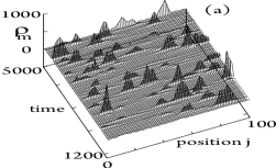
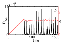
Figure 1: (a) Uncorrelated type C bands for $\dot{\varepsilon}_{a}=40$. (b) (Color online) Plots of stress and acoustic emission energy signals.

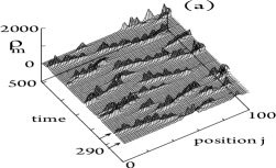
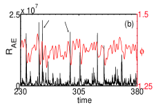
Figure 2: (a) Partially propagating type B bands for $\dot{\varepsilon}_{a}=130$. (b) (Color online) Plots of stress and acoustic emission energy signals in asymptotic regime. The region between the arrows in figures (a) and (b) are identified.

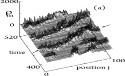
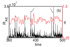
Figure 3: (a) Fully propagating type A bands at $\dot{\varepsilon}_{a}=240$. (b) (Color online) Plots of stress and acoustic emission energy signals in asymptotic regime. The region between the arrows in figures (a) and (b) are identified.

Equations (1-4) and Eq. (6) are in principle coupled since ${\dot{\varepsilon}}_{p}(y,\tau)$ is a function of stress $\phi(\tau)$. A self consistent solution of these equations is equivalent to solving the full dynamical problem involving both plastic deformation and elastic degrees of freedom with the attendant difficulties. This will not be attempted here. Instead we provide an approximate method akin to adiabatic methods. The procedure adopted is to first calculate $\dot{\varepsilon}_{p}(k,\tau)$ for the entire duration of time by solving Eqs. (1-4). Then, Eqs. (6) is solved using $\dot{\varepsilon}_{p}(k,\tau)$ as a source term (along with the scale factor $\lambda$). This gives the elastic strain $\varepsilon_{e}(y,\tau)$. Then, the integral of $\varepsilon_{e}(y,\tau)$ over the specimen dimension gives the transient stress $\phi_{tr}(\tau)$ explicitly. While $\phi_{tr}(\tau)$ will be equal to $\phi$ within the elastic limit, it will be different from $\phi$ beyond this limit.

The AK model predicts the three band types found with increasing strain rate Bhar03 ; Anan04 ; GA07 . At low ${\dot{\varepsilon}}_{a}$, say ${\dot{\varepsilon}}_{a}=40$, the uncorrelated static C bands are seen as shown in Fig. 1(a). The serrations are large and nearly regular. The scaled acoustic energy dissipated is obtained using $R_{AE}={\Gamma^{s}\over 2}\int\Big{[}{\partial\dot{\varepsilon}_{e}(y)\over\partial y}\Big{]}^{2}dy$, where $\Gamma^{s}={\Gamma}/{(\theta V_{0})^{2}}$. Since, stress drops in this case are due to isolated band nucleation, the AE pattern consists of well separated bursts that are well correlated with the stress drops. Figure 1(b) shows a typical stress-strain curve along with the AE bursts for ${\dot{\varepsilon}}_{a}=40$. The post burst AE is continuous that gradually increases until a new burst is seen ZR90 .

At intermediate strain rates, say ${\dot{\varepsilon}}_{a}=130$ hopping type B bands are seen as shown in Fig. 2(a). These propagate partially and stop mid-way. Another hopping band reappears in the neighborhood. Often, nucleation occurs at more than one location. The corresponding asymptotic stress-time plot is shown in Fig. 2(b). The associated serrations are irregular but are smaller in magnitude compared to the type C. While the correlation between stress drops and AE peaks still holds when the propagation is short, the AE bursts are not as well separated as in the case of type C serrations. A plot of the AE signal is shown in Fig. 2(b). During hoping propagation, low level AE activity is seen in the region between two AE bursts (shown by arrows) CR87 ; Ch02 ; Ch07 . (A few small bursts are also seen.) As we increase ${\dot{\varepsilon}}_{a}$, the extent of propagation increases with concomitant decrease in stress drop magnitudes. At high $\dot{\varepsilon}_{a}$ we find fully propagating type A bands. Figure 3(a) shows dislocation bands nucleating at one end of the sample and propagating continuously to other end for ${\dot{\varepsilon}}_{a}=240$. The corresponding AE pattern [Fig. 3 (b)] appears nearly continuous with a few over-riding bursts. Large bursts in AE are correlated with the nucleation of the band (or the band reaching the edge or due to occasional intersection of two bands). There is a low level AE activity during propagation (the region between the arrows). In experiments, bands once nucleated trigger a burst in AE but during propagation very low activity is seen CR87 ; Ch02 ; Ch07 . Thus, the generic features of AE signals during the PLC effect are well captured.

In summary, we have developed a theoretical frame-work for dealing with widely separated inertial time scale and that of collective dislocation modes to explain the nature of acoustic emission patterns observed in the PLC effect. This has been done by computing the plastic strain rate from the AK model for the PLC effect and using it as a source term in the wave equation. An important input in the theory is that the energy of the transient acoustic wave dissipated caused by the abrupt slip (resulting from collective unpinning of dislocations) is represented in terms of the Rayleigh dissipation function Rumiprl ; Rajeevprl . The results show that for type C bands, well separated burst type AE signals that are correlated with stress drops are seen. As we increase the strain rate successive bursts tend to merge. For high $\dot{\varepsilon}_{a}$ where type A propagating bands are seen, the bursts merge to form continuous type of AE signal. Over riding this are AE bursts that correspond to band nucleation or a band reaching the edge. These features are consistent with experimental results ZR90 ; Ch02 ; Ch07 . Other features such as those from hardening can not be captured here as there is very little hardening in the AK modelCh02 ; Ch07 . However, an extension of the AK model that removes this limitation can be used Ritupan . The frame-work is clearly applicable to other deformation conditions as long as a dislocation based model can be developed that captures major features of the phenomena. Finally, better approximate schemes have been designed that also give similar results Jag10 .

G. A acknowledges the Department of Atomic Energy grant through Raja Ramanna Fellowship Scheme and and INSA for Senior Scientist postion, and also BRNS Grant No. 2007/36/62-BRNS/2564. We thank Prof. A. S. Vasudeva Murthy for useful discussions.

References

- (1) P. R. Sammonds, P. G. Meredith and I. G. Main, Nature 359, 228 (1992).
- (2) A. Petri et al., Phys. Rev. Lett.73,3423 (1994).
- (3) E. Vives et. al., Phys. Rev. Let. 72, 1694 (1994).
- (4) R. Ahluwalia and G. Ananthakrishna, Phys. Rev. Lett. 86, 4076(2001).
- (5) M. Ciccotti, B. Giorgini, D. Villet, and M. Barquins, Int. J. Adhes. Adhes. 24, 143 (2004).
- (6) Rumi De and G. Ananthakrishna, Phys. Rev. Lett. 97, 165503 (2006).
- (7) M. C. Miguel et al., Nature 410, 667 (2001).
- (8) J. Weiss and D. Marsan, Science 299, 89 (2003).
- (9) R. M. Fisher and J. S. Lally, Can. J. Phys. 45, 1147 (1967); H. Dunegan and D. Harris, Ultrasonics 7, 160 (1969); D. R. James and S. H. Carpenter, J. App. Phys. 42, 4685 (1971).
- (10) C. H. Caceres and Rodriguez, Acta Metall. 35, 2851 (1987).
- (11) F. Zeides and J. Roman, Scipta Metall. 24, 1919 (1990).
- (12) F. Chmelik et al., Mater. Sci. Eng. A 324, 200 (2002).
- (13) F. Chmelik et al., Mater. Sci. Eng. A 462, 53 (2007).
- (14) K. Malen and L. Bolin, Phys. Stat. Sol. (b) 61, 637 (1974); B. Tirbonod, Int. J. Fracture 58, 21 (1992); B. Polyzos and A. Trochidis, Wave Motion 21, 343 (1995).
- (15) G. Ananthakrishna, Phys. Rep. 440, 113 (2007).
- (16) M. S. Bharathi, S. Rajesh and G. Ananthakrishna, Scripta Mater. 48, 1355 (2003).
- (17) G. Ananthakrishna and M. S. Bharathi, Phys. Rev. E 70, 026111 (2004).
- (18) G. Ananthakrishna and M.C. Valsakumar, J. Phys. D 15, L171 (1982).
- (19) S. Rajesh and G. Ananthakrishna, Phys. Rev. E 61, 3664 (2000).
- (20) G. Ananthakrishna and M. C. Valsakumar, Phys. Lett. A95, 69 (1983).
- (21) G. Ananthakrishna et al.,Phys. Rev. E60,5455(1999); M.S.Bharathi,et al., Phys. Rev.Lett.87,165508(2001).
- (22) L. D. Landau and E. M. Lifschitz, Theory of Elasticity (Pergamon, Oxford, 1986).
- (23) Rumi De and G. Ananthakrishna, Europhys. Lett. 66, 715 (2004).
- (24) S. Sreekala and G. Ananthakrishna, Phys. Rev. Lett. 90, 135501 (2003).
- (25) Jagadish Kumar, M. Ciccotti and G. Ananthakrishna, Phys. Rev. E 77, 045202 (2008).
- (26) Jagadish Kumar, Rumi De and G. Ananthakrishna, Phys. Rev. E 78, 066119 (2008).
- (27) R. Sarmah and G. Ananthakrishna, to be published.
- (28) Jagadish Kumar, Ph. D thesis, Indian Institute of Science, Bangalore (2010), chapter 6.