The first evidence for multiple pulsation axes: a new roAp star in the Kepler field, KIC 10195926

Abstract

We have discovered a new rapidly oscillating Ap star among the Kepler Mission target stars, KIC 10195926. This star shows two pulsation modes with periods that are amongst the longest known for roAp stars at 17.1 min and 18.1 min, indicating that the star is near the terminal age main sequence. The principal pulsation mode is an oblique dipole mode that shows a rotationally split frequency septuplet that provides information on the geometry of the mode. The secondary mode also appears to be a dipole mode with a rotationally split triplet, but we are able to show within the improved oblique pulsator model that these two modes cannot have the same axis of pulsation. This is the first time for any pulsating star that evidence has been found for separate pulsation axes for different modes. The two modes are separated in frequency by 55 $\mu$Hz, which we model as the large separation. The star is an $\alpha^{2}$ CVn spotted magnetic variable that shows a complex rotational light variation with a period of $P_{\rm rot}=5.68459$ d. For the first time for any spotted magnetic star of the upper main sequence, we find clear evidence of light variation with a period of twice the rotation period; i.e. a subharmonic frequency of $\nu_{\rm rot}/2$. We propose that this and other subharmonics are the first observed manifestation of torsional modes in an roAp star. From high resolution spectra we determine $T_{\rm eff}=7400$ K, $\log g=3.6$ and $v\sin i=21$ km s^-1. We have found a magnetic pulsation model with fundamental parameters close to these values that reproduces the rotational variations of the two obliquely pulsating modes with different pulsation axes. The star shows overabundances of the rare earth elements, but these are not as extreme as most other roAp stars. The spectrum is variable with rotation, indicating surface abundance patches.

1 Introduction

The rapidly oscillating Ap (roAp) stars are a unique laboratory in which the interaction between stellar pulsation and a magnetic field can be studied in greater detail than in any other star except the Sun. Although the pulsation periods in roAp stars are about the same as in the Sun (a few minutes), they are probably driven by the $\kappa$-mechanism in the hydrogen ionization zone, rather than being stochastically excited by convection, as in the Sun. It is thought that suppression of convection at the magnetic poles reduces damping in the hydrogen ionization zone and allows modes of high radial order to be driven (Balmforth et al., 2001).

However, when comparing theoretical instability strips to the positions of the known roAp stars in the HR diagram, there remains a difficulty in explaining the presence of pulsations in the coolest roAp stars. The theoretical red edge seems to be hotter than its observed counterpart, a fact that was noted when the first theoretical instability strip was computed (Cunha, 2002), and that is even more obvious today, with more roAp stars having reliable effective temperature determinations below 7000 K. Moreover, the agreement does not seem to improve when models with different global metallicity or local metal accumulation are considered (Théado et al., 2009). While the iron abundance may influence the excitation, it seems not to have an impact on the red edge of the theoretical instability strip.

The Ap stars have strong, global magnetic fields in the range $1-25$ kG and overabundances of some rare earth elements that can exceed $10^{6}$ of the solar value. These abundance anomalies are located in patches on the stellar surface that give rise to photometrically observable rotational light variations. The abundances are also vertically stratified in the observable atmosphere. They are thought to arise by atomic diffusion in the presence of a magnetic field. Thus Ap stars in general, and roAp stars in particular, are test beds for atomic diffusion theory, which is important for solar physics, stellar cluster age determinations, pulsation driving in main sequence and subdwarf B stars and a possible solution for frequency anomalies in $\beta$ Cep stars.

The general view of roAp stars is that the pulsation axis is not aligned with the rotation axis, thus uniquely allowing the pulsation modes to be viewed from varying aspect with rotation. This provides geometric mode identification information that is not available for other asteroseismic targets. A simple model is that the pulsation axis is aligned with the axis of the magnetic field, which is assumed to be roughly a dipole inclined with respect to the axis of rotation. As the star rotates, the geometry of the pulsation changes, leading to amplitude and, in some cases, phase modulation. This is the oblique pulsator model (Kurtz, 1982).

In early work it was assumed that the eigenfunction could be represented as a pure axisymmetric spherical harmonic, in which case the variation of pulsational amplitude with rotation leads directly to a determination of the spherical harmonic degree, $l$. Furthermore, amplitude variation also allows constraints on the relative inclinations of the rotational and magnetic axes to be placed. We now know that the eigenfunction is far from a simple spherical harmonic (Takata & Shibahashi, 1994, 1995; Dziembowski & Goode, 1996; Cunha, 2006; Saio & Gautschy, 2004; Bigot et al., 2000) and values derived in this way should be treated with caution. Treating the combined effects of rotation and magnetic field on the pulsation modes is complex. Bigot & Dziembowski (2002) showed that in the case of a relative weak global magnetic field – $B_{\rm p}\leq 1000$ G – the pulsation axis is, in general, neither the magnetic axis nor the rotation axis, but lies between these.

There are 40 roAp stars known from ground-based observations that are listed by Kurtz et al. (2006), and a few discovered more recently (see, e.g., Kochukhov et al. 2009; Elkin et al. 2010). High-resolution spectroscopy using large telescopes allows sufficient time resolution for the detailed study of line profile variations caused by rapid pulsation. It turns out that detection of low-amplitude roAp pulsations is easier using radial velocities obtained in this way rather than high-precision photometry. Several roAp stars are known in which the radial velocity variations can be detected, but no corresponding light variations can be seen from ground-based observations. A global network of spectrographs dedicated to asteroseismology, such as the SONG (Stellar Observations Network Group) project (e.g., Grundahl et al. 2009) may greatly increase the number of known roAp stars. For now, however, photometry is still the most cost-effective method for global asteroseismic studies in these stars where the frequencies are the fundamental data. For detailed examination of pulsation mode behaviour in the observable atmospheres, spectroscopic studies are superior (see, e.g., Ryabchikova et al. 2007, Freyhammer et al. 2009).

Figure 1: Top: The long cadence light curve of KIC 10195926 from Q0 + Q1. The ordinate is ${\rm BJD}-2450000$. Middle: The short cadence light curve of KIC 10195926 from Q3.3. Bottom: the short cadence light curve after high pass filtering (described in Section 4) has removed the rotational light variations, leaving only the pulsational variations. Only the envelope of the pulsation is visible here, as the pulsation period is too short to be resolved at this scale. Note that pulsation maximum coincides with rotational minimum light.

The Kepler Mission has revolutionised our ability to detect low-amplitude light variations in stars, reducing the detection limit to only a few micromagnitudes even in rather faint stars. The Kepler asteroseismic programme is described by Gilliland et al. (2010), and details of the mission can be found in Koch et al. (2010). Kepler is observing about 150 000 stars continuously over its minimum 3.5-y mission lifetime with 30-min time resolution. A small allocation (512 stars) can be studied with 1-min time resolution. While there were no known roAp stars in the Kepler field before launch in 2009, three have been found in the 1-min cadence data. KIC 8677585 was studied by Balona et al. (2010) who found several pulsation frequencies with periods around 10 min, including an unexpected low frequency of 3.142 d^-1 which is possibly a g-mode pulsation. A second roAp star discovered in the Kepler data, KIC 10483436, shows a rotational light variation and two frequency multiplets (Balona et al., in preparation).

The third roAp star discovered in the Kepler data is KIC 10195926 ($\alpha=19\,05\,27$, $\delta=+47\,15\,48$, J2000; $Kp=10.57$), which we report on here. It has a principal mode that shows a clear frequency septuplet with separations equal to the rotation period of the star, $P_{\rm rot}=5.68459$ d. Rotational light variations are clearly seen, indicating that it is an $\alpha^{2}$ CVn star. It appears that in this star both pulsation poles can be viewed over the rotation cycle, which resembles the well-studied roAp star HR 3831 (see, e.g., Kurtz et al. 1990, Kurtz et al. 1997, Kochukhov et al. 2004, Kochukhov 2006, and references therein). A second, much lower amplitude mode that shows a frequency triplet split by the rotation frequency is also found, thanks to the 5 $\mu$mag precision of the Kepler data. Interestingly, it appears that these two modes do not share the same pulsation axis, an effect that has never been detected previously. We present theoretical support for this hypothesis.

2 Fundamental parameters from spectroscopy

Spectroscopic observations of KIC 10195926 were made with the high-resolution Fibre-fed Echelle Spectrograph (FIES) at the Nordic Optical Telescope (NOT) in 2010 June, July and August. The spectra have a resolution of $R=65\,000$ and cover the spectral range $370-730$ nm. The signal-to-noise ratio (S/N) attained is about 60 for the June spectra and 40 for observations in July and August. The star was also observed with the Sandiford Echelle spectrograph on the 2.1-m telescope at McDonald Observatory. The spectra have a resolution of $R=60\,000$ and were collected on four nights in 2010 July covering the spectral region $508-605$ nm. On nights when multiple exposures were taken, they were co-added. The S/N for these observations ranges from 50 to 80. Table 1 gives a journal of the observations indicating their rotational phase (see Section 3 below).

Table 1: A journal of spectroscopic observations obtained with FIES on the Nordic Optical Telescope, and with the Sandiford Spectrograph on the McDonald Observatory 2.1-m telescope. The rotational phase has been calculated using the ephemeris $\Phi_{\rm rot}=245\,5168.91183+5.68459$.

Nordic Optical Telescope – FIES
JD $-2450000.0$	exposure time (s)	rotational phase
5369.64536	1800	0.31
5369.66862	1800	0.32
5407.37706	1800	0.95
5407.40009	1800	0.95
5408.37815	1800	0.13
5408.40118	1800	0.13
5411.68126	1800	0.71
5411.70415	1800	0.71
McDonald 2.1-m telescope – Sandiford spectrograph
5397.92206	2400	0.28
5398.69240	1800	0.42
5399.70613	1800	0.60
5400.90493	1800	0.81

Most roAp stars have strong magnetic fields in the range of $1-25$ kG. Knowledge of the magnetic field strength is important for understanding and modelling these stars. In the spectra of KIC 10195926 there is no obvious Zeeman splitting of magnetically sensitive spectral lines. We therefore searched for magnetic broadening by comparing the observations with synthetic spectra calculated for the spectral region around the Fe ii 6149.258 Å line using the SYNTHMAG program by Piskunov (1999). With the S/N of our spectra and rotational broadening, we can only place an upper limit on the magnetic field modulus of about 5 kG.

Because of the probable magnetic broadening, it is necessary to use lines with negligible Landé factors to measure the projected rotational velocity $v\sin i$. Because of the patchy distribution of elements over the surface, it is necessary to examine spectra at different rotation phases, since lines from elements concentrated in spots do not always sample the full rotation velocity of the star. From the Fe i line at 5434.523 Å we determined from spectra at different rotation phases that $v\sin i=21-24$ km s^-1. Most spectral lines are fitted well with values in this range, but some require an even smaller $v\sin i$, probably because of the spots. At some rotation phases 24 km s^-1 is needed to fit the line broadening. Our internal error on a determination of $v\sin i$ is 1 km s^-1, which we cautiously increase to 2 km s^-1. Our estimate is $v\sin i=21\pm 2$ km s^-1, but we consider this to be near a lower limit for the equatorial rotation velocity, given the larger $v\sin i$ that we see at some rotation phases.

KIC 10195926 has photometrically determined parameters from broadband photometry given in the Kepler Input Catalogue (KIC): $Kp=10.57$, $T_{\rm eff}=7400$ K, $\log g=3.6$. The KIC gives an estimate of the contamination factor for this star of 0.015, meaning that less than 1.5 percent of the light in the observing mask can be from contaminating background stars. This makes it exceedingly improbable that any of the light variations we discuss in the paper might be from a contaminating background star.

To determine the effective temperature of the star, Balmer lines profiles were compared with synthetic profiles starting with parameters close to those from Kepler Input Catalogue. Synthetic spectra were calculated with the SYNTH program of Piskunov (1992). We used model atmospheres from the NEMO database (Vienna New Model Grid of Stellar Atmospheres) (Heiter et al., 2002). This grid has an effective temperature step of 200 K, which we interpolated to get models with a 100 K step. The spectral line list for analysis and SYNTH calculations was taken from the Vienna Atomic Line Database (VALD, Kupka et al. 1999), which includes lines of rare earth elements from the DREAM database (Biémont et al., 1999).

We found a best fit for H$\alpha$ and H$\beta$ with synthetic profiles for $T_{\rm eff}=7200$ K, with estimated error of 200 K. The determination of the surface gravity is difficult at this temperature. The Balmer line profiles are relatively insensitive to $\log g$, constraining it only to within $\pm 0.5$. Ionisation equilibrium for Fe i and Fe ii lines and Cr i and Cr ii lines is potentially much more sensitive for determining $\log g$, but we did not get reliable results with our initial study. We expect a more detailed analysis, which is underway, will better constrain $\log g$. We therefore use here the photometrically determined value of $\log g=3.6$ (cgs) from the KIC. Because the spectrum is not very peculiar, we estimate a 1$\sigma$ error of $\pm 0.3$.

A detailed abundance analysis is in progress. We made preliminary estimates of the abundances of some elements at two rotation phases to get an overview of the spectral character of KIC 10195926. Using synthetic spectra calculated with SYNTH for model $T_{\rm eff}=7200$ K and $\log g=3.6$ we examined some abundances using the first and third NOT spectra listed in Table 1. The spectral lines are clearly variable with rotation, so other spectra will give values that differ for some elements. Surprisingly for a roAp star, there are no obvious lines of rare earth elements. The usual strong lines in roAp stars of Nd iii and Eu ii are present and indicate overabundances compared to the Sun, but less than is typical for most other roAp stars. Si ii lines are normal. There is no obvious core-wing anomaly (Cowley et al., 2001) in H$\alpha$, a usual signature of roAp stars.

Table 2 gives the abundances we found compared to solar values. The second column gives the abundances for a spectrum obtained at rotational phase 0.31. For this spectrum no clear evidence lines of rare earth elements was found. There are some hints of the presence of such lines in the spectrum, but the better S/N spectra are required. The fourth column gives abundances for a spectrum obtained at rotational phase 0.95. This spectrum definitely shows lines of Eu ii and a trace of weak lines of Nd iii which confirm the peculiarity of this star. Lines of strontium are much wider and stronger in this spectrum while the barium lines are much weaker when compared with the spectrum at phase 0.31. Iron lines are weaker and slightly wider with lower abundances. The spectral lines show strong variability with rotational period, demonstrating the spotted surface structure. By comparing with the roAp star HD 99563 (Freyhammer et al., 2009), we judge that lines of Eu ii and Ba ii are formed in rather small spots. Other elements also demonstrate nonuniform distribution over stellar surface. Fig. 2 shows the Eu ii 6645-Å line at four rotation phases. While better S/N is needed for further study, it is clear that Eu ii is concentrated is at least two small spots close to the pulsation pole (and hence probably close to the magnetic pole) of this star.

We note that the abundances determined here are not characteristic of the entire star. Atomic diffusion causes atmospheric stratification in Ap stars, with some elements being enhanced by orders of magnitude with respect to the Sun, while others are deficient. As a main sequence A star KIC 10195926 has an age less than 1 Gyr, hence is expected to have global abundances somewhat higher than those of the much-older Sun. This is a consideration when modelling the star.

Figure 2: This shows the Eu ii 6645 Å line at four different rotation phases. The spectra have been offset on the y-axis for visibility. The bottom spectrum is for rotation phase 0.95, which is close to the time of pulsation maximum and also rotational light minimum (see Fig. 4.) This is when one of the Eu ii spots is close to crossing the line-of-sight. In the middle panels, which are near quadrature, it is likely that two small spots of Eu ii that are concentrated near the magnetic poles are seen separately. This will be studied in detail with future, higher S/N spectra.

Table 2: Chemical abundances for KIC 10195926 and the corresponding solar abundances (Asplund et al., 2009). The errors quoted are internal standard deviations for the set of lines measured. Columns 2 and 4 give, respectively, abundances determined at two rotation phases, 0.31 and 0.95, using $P_{\rm rot}=5.68459$ d (see section 3) . The rotation phase refers to the time of pulsation maximum, which coincides with rotational light minimum as seen in Fig. 4. Columns 3 and 5 give the number of lines, ${\rm N}_{\rm l}$, used in each case.

Ion	$\log\,N/N_{\rm tot}$	${\rm N}_{\rm l}$	$\log\,N/N_{\rm tot}$	${\rm N}_{\rm l}$	$\log\,N/N_{\rm tot}$
	$\phi=0.31$		$\phi=0.95$		Sun
C i	$-3.6\pm 0.2$	2			$-3.57$
Mg i	$-4.4\pm 0.1$	3	$-4.3\pm 0.1$	4	$-4.47$
Si i	$-4.4\pm 0.2$	3	$-4.1\pm 0.1$	4	$-4.40$
Si ii	$-4.2\pm 0.1$	3	$-4.0\pm 0.2$	3	$-4.49$
Ca i	$-5.1\pm 0.1$	18	$-5.3\pm 0.2$	10	$-5.66$
Sc ii	$-8.7\pm 0.1$	3	$-9.9\pm 0.2$	2	$-8.85$
Ti ii	$-6.8\pm 0.3$	3			$-7.05$
Cr i	$-5.8\pm 0.2$	4	$-5.4\pm 0.4$	4	$-6.36$
Cr ii	$-5.7\pm 0.1$	6	$-5.7\pm 0.1$	8	$-6.36$
Fe i	$-4.3\pm 0.1$	25	$-4.6\pm 0.1$	29	$-4.50$
Fe ii	$-4.3\pm 0.1$	7	$-4.6\pm 0.1$	7	$-4.50$
Ni i	$-5.9\pm 0.1$	4	$-6.7\pm 0.2$	3	$-5.78$
Sr ii	$-8.8\pm 0.2$	2	$-8.0\pm 0.2$	2	$-9.13$
Y ii	$-8.9\pm 0.1$	2	$-8.8\pm 0.3$	5	$-9.79$
Ba ii	$-9.0\pm 0.1$	3	$-10.4\pm 0.3$	2	$-9.82$
Nd iii			$-9.3\pm 0.1$	3	$-10.58$
Eu ii			$-8.4\pm 0.1$	4	$-11.48$

3 The light curves and rotation period

KIC 10195926 has been observed by the Kepler mission during three “rolls” up to this writing. Following each quarter of a 370-d Kepler solar orbit the telescope is rolled to keep its solar panels facing the Sun. Choices and changes of targets are made on the basis of these “quarters”, which sometimes are split into approximately 1-month “thirds”. Most data (for $>$150 000 stars) are obtained in long cadence (LC) with integration times of 29.4 min. For 512 targets data are obtained in short cadence (SC) mode with sampling times just under 1-min. The three rolls for which we have data for KIC 10195926 are long cadence in Q0 (quarter zero), which was a commissioning roll of less than 10 d, long cadence in Q1, and short cadence in Q3.3 (25 d during the last third of Q3). Table 3 gives a journal of the data.

Table 3: A journal of the Kepler data for KIC 10195926. The third column is the number of data points after a few obvious outliers have been removed. The Q1 data have had a linear trend removed because of instrumental drift. The final column gives the root-mean-square variance in each data set of one point with respect to the mean. This includes all variance in noise and stellar variability.

quarter	cadence	npts	time span	rms variance
			days	$\mu$mag
Q0	LC	471	9.71	1207
Q1	LC	1621	33.45	1190
Q3.3	SC	33 679	25.07	1191

Fig. 1 shows the long cadence light curve for Q0 and Q1 together in the top panel and the short cadence light curve for Q3.3 in the middle panel. A few outlying points were edited from the raw data and a linear trend to correct for instrumental drift was removed from the Q1 data. The data are in Kepler magnitude, $Kp$, which is in broad-band white light. It is obvious from Fig. 1 that KIC 10195926 is an $\alpha^{2}$ CVn star; i.e., it has surface spots that produce a variation in brightness with rotation. This is a common feature of the magnetic Ap stars and implies that the star has a strong, global magnetic field, even though that field is yet to be detected, and we were only able to place an upper limit on it of 5 kG in Section 2. In some roAp stars, e.g. HR 3831 (Kochukhov et al., 2004) and HD 99563 (Freyhammer et al., 2009), the rare earth element surface spots are concentrated near to the pulsation or magnetic poles. These rare earth element spots often correlate with rotational light variations, particularly in the blue. With the advent of high precision space-based observations we can now see rotational light variations from spots in Ap stars that would not have been detected with ground-based observations, or at least would have given a poorly defined light curve. Such is the case for KIC 10195926 where the peak-to-peak range in $Kp$ is only slightly greater than 3 mmag. We point out, however, that the rotational light variations of Ap stars are strongly wavelength dependent, as the result of flux redistribution caused by abundance spots, so that KIC 10195926 may well show higher amplitude rotational light variations observed in filtered light such as Johnson $U$ or $B$.

To determine the rotational period of KIC 10195926 we co-added the 1-min integrations of Q3 to 30-min integrations and analysed all of the data listed in Table 3. There is a 158-d gap between the end of the Q1 data and the beginning of the Q3.3 data, giving rise to possible alias ambiguities in an analysis of the full data set. As can be seen from Fig. 1 the rotational light curve is highly nonsinusoidal, so Fourier analysis is not the best choice for period determination. We chose to fit a harmonic series by linear least-squares to the data to search for the greatest reduction in the variance in the data.

Figure 3: Top: This figure plots the standard deviation of one observation with respect to a fit of a fifth-order harmonic series at each frequency to the data. The procedure breaks down at low frequency, and is meaningless at zero frequency, hence the choice of frequency range searched. Bottom: This is a higher resolution view of the best-fitting frequency that shows there is no alias ambiguity, despite the 158-d gap in the data between Q1 and Q3.3.

Figure 4: The rotational phase curve for the Q0 and Q1 data for KIC 10195926. We have chosen the zero point of the time scale to be $t_{0}={\rm BJD}\,2455168.91183$, which is the time of pulsation maximum for the principal mode in this star. The diagram shows that pulsation maximum coincides with an extremum of the rotational light curve.

Fig. 3 shows the results of a fifth-order harmonic series fit to the data. There is a clear best frequency at $\nu_{\rm rot}=0.17591$ d^-1 with no alias ambiguity. While significant harmonics are present up to $15-20$ in the individual quarters of data, no discernible improvement in Fig. 3 can be seen with a higher-order fit.

We then fitted 20 harmonics of $\nu_{\rm rot}=0.17591$ d^-1 to the full data set by least-squares and then nonlinear least-squares to optimise the frequency and make an error estimate. This gave our best determination of the rotation frequency of $\nu_{\rm rot}=0.175914\pm 0.000004$ d^-1, which corresponds to a rotation period of $P_{\rm rot}=5.68459\pm 0.00013$ d. This error estimate is internal. Some systematic effects are still present in the data, such as small instrumental drifts and slight changes in amplitude between quarters. These will be improved in future data reductions using more detailed pixel information. Since more data for KIC 10195926 are being obtained, the rotation period will be determined to higher accuracy in future studies. The precision given here is excellent for comparison with the pulsation phases within the oblique pulsator model.

Fig. 4 shows the long cadence light curve for Q0 and Q1 phased with the rotational period. The double-wave character of the rotational light curve indicates two principal spots. The zero point of the time scale has been selected to coincide with the time of pulsation maximum, as determined in Section 4 below. It can be seen that minimum rotational brightness coincides with pulsation maximum, as is expected in the oblique pulsator model (Kurtz, 1982), in the case when the spots are associated with the magnetic/pulsation axis of the star. This coincidence can also be seen by comparing the middle and bottom panels of Fig. 1.

Figure 5: Light variation after removal of rotational modulation. The time scale is the same in both plots with time zero chosen to be BJD 2454950.000. The top panel shows the short-cadence data. Note the higher scatter at light minima and light maxima due to the roAp pulsation. The bottom panel shows the long-cadence data after correction of long-term drift. In both cases a clear variation with twice the rotational period can be seen.

The asymmetry of the light curve requires differences in spots on opposite hemispheres. It does not appear that the spots seen at rotational phase 0.5 are coincident with the second pulsation pole. The spots of Ap stars are often much more pronounced than this in filtered light (say, $UBVRI$), but are generally not studied previously in white light. An exception is $\alpha$ Cir, which was studied in white light with the star-tracker on the WIRE mission (Bruntt et al., 2009). While the rotational light curve of $\alpha$ Cir is more symmetrical, it has a similar low amplitude of only a few mmag.

Interestingly, Bruntt et al. (2009) showed that the pulsation pole for $\alpha$ Cir is not coincident with the spots. As that is the case here also for the second spot at rotation phase 0.5 of KIC 10195926, we speculate that as more precise rotational light curves are obtained for Ap stars, we will find more low amplitude rotational variation where the spots are not coincident with the magnetic poles. We also speculate that this will show a correlation with magnetic fields that are less strongly dipolar than in Ap stars with higher amplitude rotational light variations.

Figure 6: The upper panel is an amplitude spectrum of the Q3.3 short cadence data showing the low frequency spot variations. While it cannot be seen easily at this scale, the highest noise peaks have amplitudes less than 5 $\mu$mag. A high pass filter was thus run to remove all variations at frequencies less than 0.05 mHz with amplitudes greater than 5 $\mu$mag. The bottom panel shows the amplitude spectrum in the same range after the high pass filtering. Note the change from mmag to $\mu$mag between these panels.

3.1 The rotational subharmonic

When a $20^{\rm th}$-order harmonic series is fitted to the rotational light curves for the individual quarters, both Q0 and Q3.3 show a highly significant peak at $\frac{1}{2}\nu_{\rm rot}$, the subharmonic. That this appears in two independent data sets shows that it is not an artefact. The residual light variation after removal of the $20^{\rm th}$-order harmonic fit to the rotational light curve is shown in Fig. 5 where it is evident that there is periodic variability on a time scale of $2P_{\rm rot}=11.3692$ d. It is this that gives rise to the subharmonic and its harmonic in the frequency spectrum.

Ellipsoidal variables often have frequency spectra where the highest peak occurs at $2\nu_{\rm rot}$ as a consequence of a double-wave light curve with different maxima and minima. If the highest peak in the frequency spectrum were mistaken for $\nu_{\rm rot}$, then there would appear to be a subharmonic present. This is most unlikely to be the case for KIC 10195926. The light curve seen in Fig. 1 bears little resemblance to an ellipsoidal variable, and the incidence of short period binaries in magnetic Ap stars is very low. We are gathering high resolution spectra of this star to study its rotational variations. Those will be used to test for binary radial velocity variations. It is clear that the dominant rotational light variation is of the $\alpha^{2}$ CVn type, i.e. that the star is a spotted magnetic variable. If the variation with $2P_{\rm rot}$ were to be interpreted as orbital, then the rotation period would have to be half that of the orbital period, which is again unlikely.

Subharmonics are seen in stellar pulsation, most strikingly in the Kepler data for RR Lyr stars, including RR Lyrae itself (Szabó et al. 2010; Kolenberg et al. 2010). This is interpreted in terms of nonlinear effects in the pulsation, but this explanation does not apply here because we are dealing with rotation, not pulsation.

We interpret the rotational light variations in Fig. 1 to be caused by surface spots and we conclude that the rotation period of the star is $P_{\rm rot}=5.68459$ d. It is unlikely for an $\alpha^{2}$ CVn spotted rotator to have two sets of spots that are as asymmetric as those of KIC 10195926, but nearly identical on two opposite hemispheres, as would be required if the rotation period were twice the value given above. There is no known case of this amongst the $\alpha^{2}$ CVn variables.

We fitted by least-squares a harmonic series for $\frac{1}{2}\nu_{\rm rot}$. Other than $\nu_{\rm rot}$ and $\frac{3}{2}\nu_{\rm rot}$, only the harmonics of $\nu_{\rm rot}$ were significant. Thus if the subharmonic were the rotation frequency, we would have a harmonic series describing the data that included only every other harmonic. This, too, is unprecedented and unlikely.

Figure 7: Top: An amplitude spectrum over the full range of pulsation frequencies. The principal frequency multiplet around $\nu_{1}$ and its harmonic can be seen, as well as the frequency of a second mode close to the principal at $\nu_{2}$. Note that the ordinate scale is in $\mu$mag. Bottom: An amplitude spectrum over the full range of pulsation frequencies for the residuals to the fit in Table 4. One significant frequency is present at $\nu_{3}=0.365$ mHz (31.54 d^-1) with an amplitude of $6.5\pm 1.2$ $\mu$mag. This is formally significant at the 5.4$\sigma$ level, but it is a known Kepler artefact.

Figure 8: Amplitude spectra in the frequency range of $\nu_{1}$ and $\nu_{2}$. The top panel shows the multiplets of $\nu_{1}$ and $\nu_{2}$. The middle and bottom panels show them individually at higher resolution. Note the difference in the multiplet amplitude patterns, as this is significant for mode identification.

4 The pulsation frequencies

Fig. 6 shows an amplitude spectrum of the short cadence data seen in the middle panel of Fig. 1. To study the pulsation frequencies we ran a high pass filter to remove completely the rotational light variations, and any instrumental drift. This was done by sequential automatic prewhitening of sinusoids until the noise level at low frequencies matches that at higher frequencies. The highest amplitude noise peaks are less than 5 $\mu$mag, so all peaks with amplitudes greater than this at frequencies less than 0.05 mHz were removed from the data. The purpose of this high pass filter is to ensure white noise so that the error estimates for the high frequency peaks are realistic. There is no significant crosstalk between the low frequency rotational variations and the high frequency pulsational variations.

The bottom panel of Fig. 1 shows these high-pass filtered data, where it can be seen that the pulsation amplitude is modulated twice per rotation period. This is because the principal pulsation mode is a distorted dipole mode and the rotational inclination, $i$, and magnetic obliquity, $\beta$, are such that $i+\beta>90^{\circ}$, so that both poles are seen. That the maximum amplitude is different when alternating poles are presented suggests that neither $i$ nor $\beta$ is close to $90^{\circ}$.

Fig. 7 shows an amplitude spectrum over the full frequency range of variations seen in the star. The principal pulsation mode is seen at $\nu_{1}=972.58$ $\mu$Hz, and its harmonic can be seen at twice that frequency. Both of these are multiplets split by the rotation frequency. There is another pulsation mode close to $\nu_{1}$ at $\nu_{2}=919.55$ $\mu$Hz. These are the second lowest frequencies (i.e., the second longest pulsation periods) detected in roAp stars, after HD 116114 (Elkin et al., 2005), as a consequence of a relatively advanced evolutionary state of KIC 10195926. We return to this point in Sections 4.6 and 4.7 (see Fig. 16). We also note that the bright roAp star $\beta$ CrB (Kurtz et al., 2007) has a similar low pulsation frequency and also shows overabundances of Nd iii and Pr iii of only 1 dex as opposed to the typical 3 dex seen in many roAp stars – one of their characteristic signatures (Ryabchikova et al., 2004). We return to this point in Section 5.

Fig. 8 shows a higher resolution look at $\nu_{1}$ and $\nu_{2}$. The middle panel shows the multiplet of $\nu_{1}$. It is a frequency septuplet split by exactly the rotation frequency. This pattern is reminiscent of the well-studied roAp star HR 3831 (see, e.g., Kurtz et al. 1997; Kurtz et al. 1990). It is an indication of a perturbed dipole mode for which $i+\beta>90^{\circ}$, consistent with the rotational variation seen in Fig. 1 where there is a double wave. The bottom panel of Fig. 8 shows the frequency triplet of $\nu_{2}$. This is different to the pattern of $\nu_{1}$, as here the central peak has the highest amplitude. Thus $\nu_{1}$ and $\nu_{2}$ are either associated with modes of different degree, $l$, or have different pulsation axes. We return to this point in Section 4.3.

Table 4 lists the values of the derived frequencies from a non- linear least-squares fit to the data. We found the highest peak in the amplitude spectrum, then fitted it, along with all previously identified peaks, by linear least-squares to the data. We then prewhitened the data by that solution and searched the residuals for the next highest peak until the noise level was reached. After all of the frequencies shown in Table 4 were found, they were then fitted by non-linear least-squares to the high-pass filtered data set. As the noise is white for these data, the formal errors are appropriate. After prewhitening by the solution in Table 4, there is one significant peak left at 31.5 d^-1 – a known artefact in the Kepler data – as is shown in the bottom panel of Fig. 7. Otherwise there is nothing but white noise with highest peaks of 6 $\mu$mag. Fig. 9 shows the frequency multiplets for $\nu_{1}$ and $\nu_{2}$ schematically.

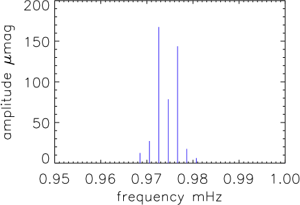
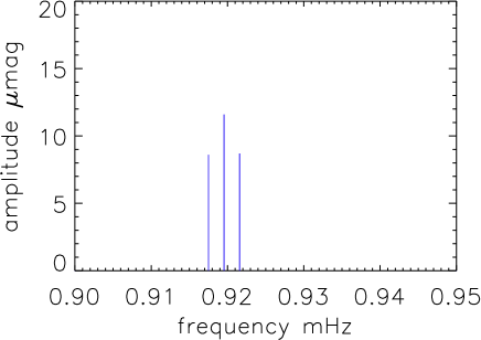
Figure 9: Schematic amplitude spectrum for the $\nu_{1}$ septuplet and $\nu_{2}$ triplet showing the component frequencies from the bottom two panels of Fig. 8. The splitting between the components of the multiplets is equal to the rotation frequency. The actual pulsation frequencies are those for the central peaks of the multiplets: $\nu_{1}=974.6183$ $\mu$Hz and $\nu_{2}=919.5464$ $\mu$Hz.

Table 4: A non-linear least-squares fit of the $\nu_{1}$ septuplet and its quintuplet harmonic, plus the $\nu_{2}$ triplet. The last column shows the frequency difference between the frequency on that line and the one on the previous line. This is the rotation frequency. The value of $\nu_{\rm rot}=2.034\pm 0.005$ $\mu$Hz translates to $P_{\rm rot}=5.690\pm 0.014$ d, which is consistent with $P_{\rm rot}=5.68459\pm 0.00013$ d derived in Section 3 from the rotational light variations. The zero point for the phases is BJD 245 5169.0. The residuals per observation for this fit equal 169.8 $\mu$mag.

ID	frequency	amplitude	phase	frequency difference
	$\mu$Hz	$\mu$mag	radians	$\mu$mag
$\nu_{2}-\nu_{\rm rot}$	$917.4581\pm 0.0367$	$8.7\pm 1.3$	$0.031\pm 0.143$
$\nu_{2}$	$919.5464\pm 0.0278$	$11.6\pm 1.3$	$2.232\pm 0.108$	$2.088\pm 0.046$
$\nu_{2}+\nu_{\rm rot}$	$921.6244\pm 0.0366$	$8.8\pm 1.3$	$-1.797\pm 0.143$	$2.078\pm 0.046$
$\nu_{1}-3\nu_{\rm rot}$	$968.5151\pm 0.0260$	$12.5\pm 1.3$	$-1.803\pm 0.100$
$\nu_{1}-2\nu_{\rm rot}$	$970.5569\pm 0.0121$	$27.3\pm 1.3$	$-2.308\pm 0.046$	$2.042\pm 0.029$
$\nu_{1}-\nu_{\rm rot}$	$972.5845\pm 0.0020$	$167.5\pm 1.3$	$-1.757\pm 0.008$	$2.028\pm 0.012$
$\nu_{1}$	$974.6183\pm 0.0043$	$78.6\pm 1.3$	$-1.438\pm 0.016$	$2.034\pm 0.005$
$\nu_{1}+\nu_{\rm rot}$	$976.6569\pm 0.0023$	$143.7\pm 1.3$	$-1.563\pm 0.009$	$2.039\pm 0.005$
$\nu_{1}+2\nu_{\rm rot}$	$978.7346\pm 0.0181$	$17.9\pm 1.3$	$-0.390\pm 0.070$	$2.078\pm 0.018$
$\nu_{1}+3\nu_{\rm rot}$	$980.7187\pm 0.0520$	$6.2\pm 1.3$	$-0.968\pm 0.201$	$1.984\pm 0.055$
$2\nu_{1}-2\nu_{\rm rot}$	$1945.0322\pm 0.0513$	$6.3\pm 1.3$	$2.462\pm 0.199$
$2\nu_{1}-\nu_{\rm rot}$	$1947.2577\pm 0.0666$	$4.9\pm 1.3$	$2.367\pm 0.255$	$2.226\pm 0.084$
$2\nu_{1}$	$1949.2662\pm 0.0246$	$13.4\pm 1.3$	$2.777\pm 0.094$	$2.009\pm 0.071$
$2\nu_{1}+\nu_{\rm rot}$	$1951.2577\pm 0.0564$	$5.8\pm 1.3$	$-2.740\pm 0.217$	$1.991\pm 0.062$
$2\nu_{1}+2\nu_{\rm rot}$	$1953.2500\pm 0.0753$	$4.3\pm 1.3$	$2.942\pm 0.290$	$1.992\pm 0.094$
$\nu_{1}-\nu_{2}$	$55.072\pm 0.028$

4.1 The principal pulsation mode and the oblique pulsator model

The separation of all the multiplets is consistent with the rotation frequency determined from the rotational light variations, as is expected in the oblique pulsator model. We therefore adopt the rotational frequency determined in Section 3, which is $\nu_{\rm rot}=2.03604\pm 0.00005$ $\mu$Hz. We tested the hypothesis that the rotation period may be $2P_{\rm rot}$, by fitting by least-squares a 13-multiplet split by the subharmonic frequency, $\frac{1}{2}\nu_{\rm rot}$, as the $\nu_{1}$ multiplet. None of the additional peaks between those seen in Fig. 9 has an amplitude more than 2.5 $\mu$mag, hence all lie well below the highest noise peaks of 6 $\mu$mag. There is thus nothing in the pulsation modulation with rotation to suggest that $2P_{\rm rot}$ might be the rotation period.

The frequency septuplet of $\nu_{1}$ of KIC 10195926 is very similar to that of HR 3831 (Kurtz et al., 1990, 1997), which is interpreted as arising from a distorted dipole mode. Kurtz (1992) showed that the mode in HR 3831 is primarily an oblique dipole mode from a spherical harmonic decomposition of its frequency septuplet. Kochukhov (2004) found that both dipole and octupole components are needed to describe the radial velocity variations in HR 3831. These results do not imply that both dipole and octupole modes are excited. There is only one mode, but the magnetic distortion of that mode from a normal mode can be described with multiple spherical harmonic components. Dziembowski & Goode (1996), Bigot et al. (2000), Cunha & Gough (2000) and Saio (2005) show theoretically how the effect of a dipole magnetic field leads to this distortion of the pulsation mode. Saio (2005 – his Fig. 12) specifically shows a comparison of the latitudinal and horizontal displacements from his model with the observational results of Kochukhov (2004) for HR 3831.

However, as in the well known roAp stars HR 3831, HR 1217 and $\alpha$ Cir, the frequencies of the modes in KIC 10195926 appear dominantly to be triplets in photometry. Whether the latitudinal magnetic distortion is weak or strong, the mode geometry can be reasonably described by a dipole mode, since the higher order components (such as $l=3$) have low visibility when averaged over the disk. For a dipole triplet, the phases of all three frequencies should be equal at the time of pulsation maximum for a simple oblique dipole mode, i.e. $\phi_{-1}=\phi_{+1}=\phi_{0}$ at that time. In Table 5 we have chosen $t_{0}={\rm BJD}\,245\,5168.91183$ to force $\phi_{-1}=\phi_{+1}$. We then note that $\phi_{0}$ differs from the value of $\phi_{-1}$ and $\phi_{+1}$ by only $0.22\pm 0.02$ rad. While this is significant (and is a result of the magnetic distortion of the mode), it is close enough to support an approximation of the central triplet as arising from a simple oblique dipole mode. We also note that Fig. 4 shows that this time corresponds to the rotational light minimum, showing that the abundance spot that gives rise to this minimum is in the plane defined by the rotation and pulsation poles. This is confirmed in the phase curve of the principal pulsation mode $\nu_{1}$ shown in Fig. 10. We found the amplitude and phase of this mode by fitting $\nu_{1}$ to consecutive 5 cycles of data. We have plotted that against rotation phase using the same zero point as in Fig. 4. The amplitude modulation and $\pi$-radian phase reversal are characteristic of an oblique dipole pulsation mode (Kurtz 1982).

The magnetic field present in roAp stars partially raises the $(2l+1)$ degeneracy of non-magnetic modes whose properties (frequency, amplitude, phase) then depend on the absolute value of their azimuthal order $m$. The modes can be either aligned or perpendicular to the field axis. However, in roAp stars, rotation is enough to play an important role in the mode properties. Indeed, since the magnetic and rotation axes are in general not aligned ($\beta\neq 0$), the rotation acts as an asymmetric perturbation on the magnetic modes, which are thereby coupled with respect to the azimuthal order (rotation is not strong enough in roAp stars to couple modes of different degrees $l$).

In this case of rotationally coupled magnetic modes the dipole mode displacement vector describes an ellipse during the pulsation period which is defined by its two axes: the X-axis in the plane defined by the rotation and magnetic axes and the other, the Y-axis, perpendicular to this plane. This is the generalized oblique pulsator model presented by Bigot & Dziembowski (2002). The mode is then fully described by the inclination of the ellipse that we defined here by the inclination $\gamma$ of the X-axis with respect to the rotation axis and the angle $\psi$ whose tangent is the ratio between the lengths of the Y- and X- axes; see Bigot & Dziembowski (2002) and Bigot & Kurtz (2010) for more details. For a pure $m=0$ dipole mode in the magnetic reference system we have $\gamma=\beta$ and $\psi=0$. For a pure $m=\pm 1$ mode in the same frame we have $\gamma=\pi/2+\beta$ and $\psi=\pm\pi/4$. The light curves (or the triplet in the frequency domain) are described by only three angles: $i,\gamma,\psi$ (Bigot & Kurtz 2010). The last two angles are functions of the magnetic field, rotation, $\beta$ and frequency.

The strength of the centrifugal force coupling of the magnetic modes depends on the frequency difference between the magnetic modes $m=0$ and $m=\pm 1$ and the centrifugal shift of frequency. In order to measure the effects, Bigot & Dziembowski (2002) defined the parameter $\left|\mu^{\rm mag}\right|$ to be the ratio between the magnetic frequency shift divided by the centrifugal shift: $\left|\mu^{\rm mag}\right|<1$ corresponds to a dominating rotation regime, $\left|\mu^{\rm mag}\right|=1$ corresponds to strong coupling, $\left|\mu^{\rm mag}\right|>1$ corresponds to a magnetic regime where there is almost no coupling. The Coriolis force is far weaker than the centrifugal force in roAp stars and almost does not enter into the balance that defines the inclination of the mode. However, it plays a role in the asymmetry of the amplitudes $A_{+1}$ and $A_{-1}$.

We do not know the magnetic field ($B_{p},\beta$) configuration for this star; thus far we have only been able to limit the polar field strength to be less than 5 kG. Because rotation is not strong enough to couple modes of different $l$, the presence of latitudinal distortion of the mode, seen as a septuplet for $\nu_{1}$, is only due to the magnetic field and can be used as a constraint on the field strength. This is what is done in the following Section 4.2. The effect of rotation is taken into account in Section 4.3.

Table 5: A linear least-squares fit of the $\nu_{1}$ septuplet and its quintuplet harmonic, plus the $\nu_{2}$ triplet. The rotation frequency has been forced to be equal to 2.034 $\mu$Hz for the splittings of the multiplets. This is to test the phase relationships. The time zero point is BJD 245 5168.91183; it has been chosen to force the phases $\phi(\nu_{1}-\nu_{\rm rot})=\phi(\nu_{1}+\nu_{\rm rot})$, Notably, the phase $\phi(\nu_{1}$) is close to the same value. Exact equality and only a frequency triplet is what is expected for a pure oblique dipole with no magnetic perturbation. The residuals per observation for this fit equal 169.8 $\mu$mag.

ID	frequency	amplitude	phase
	$\mu$Hz	$\mu$mag	radians
$\nu_{2}-\nu_{\rm rot}$	$917.5104$	$8.6\pm 1.3$	$0.120\pm 0.145$
$\nu_{2}$	$919.5464$	$11.6\pm 1.3$	$2.200\pm 0.108$
$\nu_{2}+\nu_{\rm rot}$	$921.5824$	$8.7\pm 1.3$	$-1.964\pm 0.144$
$\nu_{1}-3\nu_{\rm rot}$	$968.5102$	$12.4\pm 1.3$	$2.110\pm 0.100$
$\nu_{1}-2\nu_{\rm rot}$	$970.5462$	$27.2\pm 1.3$	$1.503\pm 0.046$
$\nu_{1}-\nu_{\rm rot}$	$972.5822$	$167.4\pm 1.3$	$1.955\pm 0.007$
$\nu_{1}$	$974.6183$	$78.6\pm 1.3$	$2.176\pm 0.016$
$\nu_{1}+\nu_{\rm rot}$	$976.6543$	$143.8\pm 1.3$	$1.956\pm 0.009$
$\nu_{1}+2\nu_{\rm rot}$	$978.6904$	$17.6\pm 1.3$	$3.041\pm 0.071$
$\nu_{1}+3\nu_{\rm rot}$	$980.7264$	$6.2\pm 1.3$	$2.343\pm 0.203$
$2\nu_{1}-2\nu_{\rm rot}$	$1945.1645$	$5.6\pm 1.3$	$-2.893\pm 0.222$
$2\nu_{1}-\nu_{\rm rot}$	$1947.2005$	$4.9\pm 1.3$	$-2.772\pm 0.258$
$2\nu_{1}$	$1949.2366$	$13.1\pm 1.3$	$-2.551\pm 0.095$
$2\nu_{1}+\nu_{\rm rot}$	$1951.2726$	$5.7\pm 1.3$	$-1.891\pm 0.221$
$2\nu_{1}+2\nu_{\rm rot}$	$1953.3087$	$4.4\pm 1.3$	$-2.573\pm 0.286$

Figure 10: This shows the amplitude and phase modulation as a function of rotational phase for $\nu_{1}$. It has been created by fitting 5 cycles of data by linear least squares for $\nu_{1}$. Notice the $\pi$ radian reversal at quadrature; this is a typical sign of dipole pulsation in an oblique pulsator. The difference in amplitude of the two maxima is a function of the different aspects as the pulsation pole crosses the stellar meridian. Rotation phase zero is the same as in Fig. 4, .i.e., with respect to $t_{0}={\rm BJD}\,2455168.91183$.

Table 6: We list all possible values of $(i,\beta)$ that lead to an inclination of the dipole mode $\nu_{1}$ in agreement with the amplitude ratio defined by the data in Table 5, i.e. $(A_{+1}+A_{-1})/A_{0}=3.96\pm 0.07$. We assume equal magnetic and centrifugal strength $\left|\mu^{\rm mag}\right|=1$. Columns 1 and 2 list the values of $i$ and $\beta$, respectively. Column 3 lists the value of the inclination $\gamma$. Column 4 lists the inclination of the dipole axis with respect to the magnetic field. Column 5 lists the corresponding polarization ($\psi=0$ is linear). Columns 6 and 7 list the angles made by the pulsation axis with the line of sight at the time of amplitude maxima. Column 8 lists the quantity $\cal{D}$ defined in Bigot & Dziembowski (2002) to measure the alignment with the magnetic field axis ($\cal{D}={\rm 0}$ means alignment). The rows in bold characters corresponding to $i=[62^{\circ},65^{\circ}]$ lead to an amplitude ratio $(A_{+1}-A_{-1})/(A_{+1}+A_{-1})$ equal to the observed one. All angles are given in degrees.

$i$	$\beta$	$\gamma$	$\gamma-\beta$	$\psi$	$\alpha(0)$	$\alpha(\pi)$	$\cal{D}$
2	89	89.50	0.50	-2.57	-87.50	91.50	0.00
6	86	88.50	1.50	-2.57	-82.50	94.50	0.00
19	80	85.01	5.01	-2.60	-66.01	104.01	0.01
24	77	83.51	6.51	-2.62	-59.51	107.51	0.01
29	74	82.01	8.01	-2.65	-53.01	111.01	0.02
32	72	81.01	9.01	-2.67	-49.01	113.01	0.03
36	68	79.51	10.51	-2.71	-43.51	115.51	0.04
39	67	78.51	11.51	-2.74	-39.51	117.51	0.04
41	65	77.51	12.51	-2.77	-36.51	118.51	0.05
43	62	76.52	13.52	-2.80	-32.52	120.52	0.06
46	61	75.52	14.52	-2.84	-29.52	121.52	0.07
48	59	74.52	15.52	-2.89	-26.52	122.52	0.07
50	55	73.02	17.02	-2.96	-23.02	123.02	0.09
51	54	72.52	17.52	-2.99	-21.52	123.52	0.09
53	53	71.53	18.53	-3.05	-18.53	124.53	0.10
53	52	71.03	19.03	-3.08	-17.03	125.03	0.11
55	49	69.53	20.53	-3.19	-13.53	125.53	0.13
57	48	69.03	21.03	-3.23	-12.03	126.03	0.13
59	43	67.04	23.04	-3.40	-8.04	126.04	0.16
60	42	66.05	24.05	-3.50	-6.05	126.05	0.17
61	41	65.55	24.55	-3.56	-4.55	126.55	0.18
62	37	63.56	26.56	-3.81	-0.56	126.56	0.20
65	33	61.58	28.58	-4.13	3.42	126.58	0.23
66	31	60.59	29.59	-4.33	5.41	126.59	0.25
67	29	59.61	30.61	-4.55	7.39	126.61	0.26
68	26	58.13	32.13	-4.95	9.87	126.13	0.29
70	20	55.23	35.23	-6.10	14.77	125.23	0.34
71	16	53.36	37.36	-7.34	17.64	124.36	0.38
72	4	51.85	47.85	-22.91	20.15	123.85	0.62
72	14	52.47	38.47	-8.22	19.53	124.47	0.40
73	6	50.38	44.38	-16.82	22.62	123.38	0.53
73	8	50.39	42.39	-13.26	22.61	123.39	0.48
73	10	50.91	40.91	-10.96	22.09	123.91	0.45

4.2 A pure magnetic model for the principal pulsation mode

Using the formalism of Saio (2005) we have solved for the effect of a dipole magnetic field on the $\nu_{1}$ mode. In this formalism the mode is assumed to be a pure $m=0$ mode with its axis of symmetry aligned with the magnetic axis; i.e. $\gamma=\beta$. We have run a set of models with appropriate $T_{\rm eff}$, $\log g$. Unperturbed evolutionary models were calculated by the OPAL opacity with a standard chemical composition of $(X,Z)=(0.7,0.02)$. Convective energy flux in the envelope is neglected assuming a strong magnetic field suppresses the convection. Helium is assumed to be depleted above the first ionization zone, treating it in the same way as in Saio et al. (2010).

Here, disregarding the effect of rotation, we assume the pulsations to be axisymmetric with respect to the axis of a dipole magnetic field which is inclined to the rotation axis by an angle of $\beta$. The eigenfunction of a pulsation mode is expressed by a sum of terms proportional to Legendre functions with different values of $\ell$. Solving numerically the differential equations for linear non- adiabatic oscillations including the effects of Lorentz forces, we obtain an eigenfrequency and the corresponding eigenfunction; i.e., the relative amplitude of each component of the expansion as a function of the depth in the envelope, which determines the latitudinal dependence of the pulsation. The latitudinal dependence of the luminosity perturbation on the surface predicts the rotational modulation of the pulsation amplitude (see Saio & Gautschy (2004) and Saio (2005) for details).

Good fits to the observed amplitude structure seen in Fig. 9 and the amplitude and phase variations as a function of rotation seen in Fig. 10 were found with a model with $M=1.70$ M_⊙, $\log L/{\rm L}_{\odot}=0.998$, $\log T_{\rm eff}=3.854$, $\log R/{\rm R}_{\odot}=0.314$ and $\log g=4.04$. Two good matches to the observations were found, one with $B_{p}=0.7\pm 0.2$ kG and the other with $B_{p}=15\pm 2$ kG. Our high resolution spectra clearly rule out a polar field strength as large as 15 kG, since that would produce clear Zeeman splitting, which is not observed, leaving only the model with $B_{p}=0.7$ kG. For the latter model, agreement with the observed pulsation amplitude and phase variations requires that $\gamma=\beta=66^{\circ}$ and $i=62^{\circ}$.

Figure 11: This shows the model pulsation amplitude and phase as a function of rotation phase for an $n=16$ dipole mode with a frequency of $\nu=978.9$ $\mu$Hz, close to the observed $\nu_{1}=974.6$ $\mu$Hz, and with $i=62^{\circ}$, $\gamma=66^{\circ}$, in good agreement with the oblique pulsator model constraints given in Table 6.

Fig. 11 shows the model amplitude and phase variations as a function of rotation phase for an $n=16$ dipole mode, in good agreement with the observations shown in Fig. 10. Fig. 12 compares the observed amplitudes of the multiplet structure with the observations. A higher than normal value of the limb-darkening coefficient of $\mu=0.8$ was needed to get good agreement for the $A_{\pm 2}$ and $A_{\pm 3}$ components. The eigenfunction shown in the bottom panel is significantly deformed from the Legendre function $P_{1}(\cos\theta)$, even though $A_{\pm 2}$ and $A_{\pm 3}$ are much smaller than $A_{1}$ and $A_{0}$. This is because for an odd mode such as a dipole mode, $l\geq 3$ components (which produce the $A_{\pm 2}$ and $A_{\pm 3}$ sidelobes) are visible only through the limb-darkening effect; without limb- darkening these components would not be visible due to cancellation on the surface. This increased limb-darkening coefficient is consistent with the atmospheric temperature gradient in roAp stars, which is steeper than in normal stars, as is usually shown by the core-wing anomaly in the Balmer lines (Cowley et al., 2001) for most roAp stars.

Figure 12: Top: A schematic amplitude spectrum for the model frequencies for $\nu_{1}$. The solid lines show the model amplitudes, while the dotted lines (displaced in frequency for visibility) show the observed amplitudes. Bottom: The latitudinal dependence of the eigenfunction. The dotted line shows pure dipole eigenfunction.

4.3 Rotational distortion of the magnetic mode $\nu_{1}$

The magnetic field derived in the previous section is rather weak for roAp stars and its effect on the mode inclination can be balanced by the centrifugal force. In this case, as shown by Bigot & Dziembowski (2002), there is no reason to have an axis of pulsation aligned along the magnetic axis or the rotation axis. In order to calculate the mode inclination $\gamma$ and its polarization $\psi$, we assume a value of $\left|\mu^{\rm mag}\right|=1$ (ratio of magnetic to centrifugal shift of frequency). The ratio $\chi$ between the Coriolis and centrifugal shift is proportional to $\sim n^{-3}\Omega^{-1}$, where $n$ is the number of radial nodes of the mode. Since $\nu_{1}$ has a lower frequency and lower $n$ than in HR 3831, the value of $\chi$ is larger than for HR 3831. From the stellar model and eigenfunctions used in Section 4.2, we find $\chi=0.045$.

Determining the mode inclination from light curves depends strongly on the viewing aspect of the mode, i.e. the value of $i$. Indeed, we found several solutions ($i,\beta$) leading to a fit of the amplitude ratio $(A_{+1}+A_{-1})/A_{0}$, as long as $i<72^{\circ}$ – see Table 6. The values follow roughly the law $i+\beta\approx 80-100^{\circ}$. While the angles derived in Table 6 lead to the same goodness of fit to the light curve, they lead to completely different values of the dipole inclination $\gamma$. Indeed, low values of $i$ lead to a dipole almost aligned with the magnetic axis, whereas large values lead to a very inclined mode: e.g. $\gamma(i=19^{\circ},\beta=80^{\circ})=85^{\circ}$, $\gamma(i=41^{\circ},\beta=65^{\circ})=77^{\circ}$ and $\gamma(i=62^{\circ},\beta=37^{\circ})=64^{\circ}$. In all cases, the polarization remains small showing that this mode is almost linearly polarized. Due to the uncertainty in $i$, it is hard to reach a conclusion about the inclination of the principal mode in KIC 10195926. The same problem appeared in the case of HR3831. Bigot & Dziembowski (2002) found a mode well inclined with respect to the magnetic axis $\gamma-\beta\approx 26^{\circ}$ based on a value of $i=89^{\circ}$ available from spectropolarimetry at this time. A more recent and secure value of $i=68^{\circ}$ in HR 3831 led Bigot & Kurtz (2010) to a mode almost aligned with the magnetic axis $\gamma-\beta\approx 0$. The alignment between magnetic and pulsation axes in HR 3831 seems natural regarding the large magnetic field found for the star $\sim 2.5$ kG. In KIC 10195926 the lower value of $B_{p}=0.7$ kG derived in Section 4.2 suggests a more inclined mode to the magnetic field.

We can extract more constraints on the inclination by considering the inequality of the side peaks $A_{+1}\neq A_{-1}$. The origin of the inequality is due to the Coriolis force which, unlike the magnetic and centrifugal forces, does not act in the same way on the $\pm m$ components of the modes. The ratio $(A_{+1}-A_{-1})/(A_{+1}+A_{-1})$ is therefore very sensitive to the value of $\chi$ which determines the polarization of the mode (Bigot & Dziembowski, 2002). It also depends on the magnetic field and centrifugal forces. Using the constraint on the unequal amplitude ratio, we restrict the allowed values of the rotational inclination and magnetic obliquity to $i\approx 63^{\circ}$ and $\beta\approx 34^{\circ}$. The mode is well inclined to the magnetic axis with $\gamma-\beta\approx 26^{\circ}$. We used the formalism developed in Bigot & Kurtz (2010) to fit of the light curve of $\nu_{1}$. An example is shown in Fig. 13 for ($i=62^{\circ}$, $\beta=63^{\circ}$).

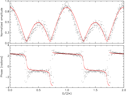
Figure 13: Amplitude (top panel) and phase (bottom panel) of the light curve variation corresponding to the mode $\nu_{1}$ as function of the rotation phase. The full line corresponds to a mode tilted to the magnetic axis by $27^{\circ}$ with a small polarization ($-4^{\circ}$); $i=63^{\circ}$.

4.4 The observed amplitude

The peak pulsation amplitude of KIC 10195926 occurs at rotation phase zero in Fig. 1. The highest amplitude occurs when the central three frequencies of the septuplet are in phase, which gives $(A_{-1}^{(1)}+A_{0}^{(1)}+A_{+1}^{(1)})=(168+79+144)$ $\mu$mag $\approx 0.4$ mmag, as is seen in Fig. 10. This is potentially detectable in ground-based observations, but not easily. However, this is the Kepler white light bandpass amplitude. A study of the roAp star $\alpha$ Cir using the WIRE satellite star-tracker by Bruntt et al. (2009) in comparison with simultaneous ground-based photometry through a Johnson $B$ filter found a weighted mean amplitude ratio of $A_{B}/A_{\rm WIRE}=2.3\pm 0.1$. If we assume that the ratio $A_{B}/A_{\it Kepler}$ is similar, then the maximum amplitude that would be observed for KIC 10195926 in $B$ is expected to be 0.9 mmag, or peak-to-peak nearly 2 mmag. There are many other roAp stars known with similar small amplitudes (see Table 1 of Kurtz et al. 2006).

Columns 6 and 7 of Table 6 give the angle between the line-of- sight and the pulsation pole for various possible geometries for KIC 10195926. These show that an implausibly high intrinsic amplitude greater than 20 mmag – more than is observed in any roAp star – would be needed if $i$ were less than $\approx 10^{\circ}$, so those geometries can be ruled out since $1/\cos(\alpha(0))$ and $1/\cos(\alpha(\pi))$ are too large ($>10$).

From the spectroscopically derived values we found in Section 2 of $T_{\rm eff}=7200$ K and $\log g=3.6$, we estimate that $R=3.6$ R_⊙. With the known rotation period $P_{\rm rot}=5.6836$ d, this radius gives $v_{\rm rot}=32$ km s^-1. With the measured $v\sin i=21$ km s^-1, we then find $i\sim 40^{\circ}$. Although there are substantial uncertainties in this estimate, the angles in Table 6 suggest that we are seeing nearly the full intrinsic amplitude of KIC 10195926 at rotation phase of best aspect.

If we use the radius and inclination of our best-fitting model from Section 4.2, $R=2.1$ R_⊙ and $i=62^{\circ}$, then we find that we expect $v\sin i=17$ km s^-1. While the errors involved are relatively large, this suggests that the model radius and gravity are too low, and the spectroscopically derived values from Section 2 are more probable.

4.5 The harmonic frequencies of $\nu_{1}$

Fig. 14 shows a schematic amplitude spectrum for the quintuplet centred on $2\nu_{1}$. Since the frequency of the central component is twice the frequency of the central component of the principal mode septuplet, it appears to be the first harmonic of the principal pulsation mode $\nu_{1}$. Since the principal mode $\nu_{1}$ is also linearly polarized along a fixed axis in the plane defined by the magnetic and rotation axes, we can consider that it is an $m=0$ mode with an axis inclined by $\gamma$ with respect to rotation axis.

We therefore use the formalism developed by Kurtz et al. (1990) for nonlinear dipole oscillations in roAp stars and replace $\beta$ by $\gamma$. We then expect

$${{A_{+2}^{(2\nu_{1})}+A_{-2}^{(2\nu_{1})}}\over{A_{+1}^{(2\nu_{1})}+A_{-1}^{(2\nu_{1})}}}={{1}\over{4}}\tan i\tan\gamma.$$ (1)

From the data in Table 4 we find for $\nu_{1}$ that $(A_{+1}^{(\nu_{1})}+A_{-1}^{(\nu_{1})})/A_{0}^{(\nu_{1})}=\tan i\tan\gamma=3.96\pm 0.07$. Substituting this value into the above formula leads to $(A_{+2}^{(2\nu_{1})}+A_{-2}^{(2\nu_{1})})/(A_{+1}^{(2\nu_{1})}+A_{-1}^{(2\nu_{1})}))\simeq 1$, which is consistent with the observations.

The amplitude ratios between the central component of the quintuplet of $2\nu_{1}$ and the side components are given by Eqs 25 and 26 of Kurtz et al. (1990). If we define by $x=\tan i\tan\gamma$ then we have $\left(A_{+1}^{(2\nu_{1})}+A_{-1}^{(2\nu_{1})}\right)/A_{0}^{(2\nu_{1})}=x^{2}/(x^{2}+2)$ and $\left(A_{+2}^{(2\nu_{1})}+A_{-2}^{(2\nu_{1})}\right)/A_{0}^{(2\nu_{1})}=4x/(x^{2}+2)$. We find for both ratios $\approx 0.89$, which is again fully consistent with the observations.

It is reasonable to conclude from these considerations that the quintuplet centred on $2\nu_{1}$ is indeed the first harmonic of the principal pulsation mode $\nu_{1}$. It is potentially possible to derive the values of $i$, $\beta$ and $\mu$ from the amplitude ratios of the multiplets of the principal mode $\nu_{1}$, the secondary mode $\nu_{2}$, and the harmonic $2\nu_{1}$.

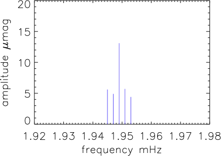
Figure 14: Schematic amplitude spectrum for the $2\nu_{1}$ harmonic quintuplet.

4.6 The secondary mode and the frequency spacing

While the frequency septuplet of the primary mode is consistent with our model and values of $i$ and $\beta$, the secondary frequency triplet of $\nu_{2}$ is problematic. From the data in Table 4 we find for $\nu_{1}$ that $(A_{+1}^{(\nu_{1})}+A_{-1}^{(\nu_{1})})/A_{0}^{(\nu_{1})}=3.96\pm 0.07$, which is significantly different to the value for $\nu_{2}$ of $(A_{+1}^{(\nu_{2})}+A_{-1}^{(\nu_{2})})/A_{0}^{(\nu_{2})}=1.51\pm 0.23$. This indicates that the two modes either arise from different spherical degrees, $l$, or have different pulsation axes.

We filtered all but the $\nu_{2}$ triplet from the data, then calculated amplitude and phase modulation of that with respect to rotation phase. Because of the smaller amplitude, we needed to use 20 cycles for each fit, rather than the 5 we used for $\nu_{1}$. Fig. 15 shows the results. Amplitude maximum occurs at rotation phase 0.67. There is an appearance of perhaps another maximum around rotation phase 0.15; this is probably real, since the rotational sidelobes sum to more than the amplitude of the central peak of the triplet, hence two maxima per rotation are expected. That the rotational phase of amplitude maximum does not coincide with that for $\nu_{1}$ supports the suggestion that the two modes are either of different spherical degree, or have different pulsation axes. We also re-ran the least squares fit of Table 5, but shifted the zero point in time to get phase equality for the $\nu_{2}$ triplet, as shown in Table 7. All three frequencies show the same phase within the errors for a time of maximum at rotational phase 0.67. This is consistent with Fig. 15.

Table 7: This table is the same as the part of Table 4 concerning $\nu_{2}$, except the zero point in time has been chosen to give phase equality for the components of the $\nu_{2}$ multiplet. This time zero point is BJD 245 5172.70203; it differs from the time of maximum for $\nu_{1}$ by 3.7902 d, or 0.67 rotation periods. The other frequencies were included in the fit, but are not shown here, as only their phases have changed from Table 4; they are no longer informative with this different time zero point.

ID	frequency	amplitude	phase
	$\mu$Hz	$\mu$mag	radians
$\nu_{2}-\nu_{\rm rot}$	$917.5126$	$8.6\pm 1.3$	$3.02\pm 0.15$
$\nu_{2}$	$919.5464$	$11.6\pm 1.3$	$3.00\pm 0.11$
$\nu_{2}$ + $\nu_{\rm rot}$	$921.5801$	$8.6\pm 1.3$	$3.02\pm 0.15$

Figure 15: Top: This shows the amplitude modulation as a function of rotational phase for $\nu_{2}$. It has been created by fitting 20 cycles of data by linear least squares for $\nu_{2}$. Notice that the amplitude is modulated only once per cycle; both amplitude and phase are poorly defined away from amplitude maximum, which occurs around rotation phase 0.67.

The separation of $\nu_{1}$ and $\nu_{2}$ is $\nu_{1}-\nu_{2}=55.07\pm 0.03$ $\mu$Hz. The model presented in Section 4.2 has a large separation $\Delta\nu_{0}\approx 57$ $\mu$Hz, which is close enough to the observed separation to suggest that $\nu_{2}$ is also a dipole mode. If that is true, then the two modes do not have the same pulsation axis. On the other hand, if we dismiss the model and conclude that the degrees of the two modes are of different parity, then 55 $\mu$Hz cannot be the large separation.

From $T_{\rm eff}=7200$ K and $R=3.6$ R_⊙, we have $\log T_{\rm eff}=3.86$ and $\log L/{\rm L}_{\odot}=1.5$. From a grid of non-magnetic models constructed using the stellar evolution code CESAM (Morel, 1997) and corresponding pulsation frequencies computed with the code ADIPLS (Christensen-Dalsgaard, 2008), we find that a model with these global properties has a large separation of 25 $\mu$Hz. On the other hand, a large separation of about 2/3 of the observed value is realized by a slightly less luminous model, with $\log L/{\rm L}_{\odot}=1.3$, and similar effective temperature. With the case for $\nu_{1}$ being a dipole mode, a plausible alternative is thus that $\nu_{2}$ is a radial or quadrupole mode and that the star is more luminous than what would be expected by assuming the observed separation to be the large separation, having, instead, $\Delta\nu_{0}\sim 37$ $\mu$Hz. In this case the two observed modes are not consecutive in radial overtone; i.e., there is a mode between them that is not excited to observable amplitude. This is seen in another roAp star, HD 217522 (Kreidl et al., 1991), so is not without precedent. The difficulty with this solution, when considering the effect of a dipolar magnetic field on the oscillations, is that the magnetic distortion of the eigenfunctions of even degree modes always generates an $l=0$ component. Even when this component is comparably smaller than the $l=2$ component, after averaging over the disk its impact is significant. In particular, we were not able to find a magnetic model within the scenario of $\nu_{2}$ being of degree $l=2$, in which the pulsation phase of this second mode jumps by an amount comparable to that seen in the observations at particular rotation phases.

Fig. 15 shows that maximum amplitude for $\nu_{2}$ is at rotation phase 0.67; this is definitely different from the maximum phase of $\nu_{1}$. Thus the rotational phase of maximum and the multiplet amplitude ratios for $\nu_{1}$ and $\nu_{2}$ are clearly different, yet $\nu_{1}-\nu_{2}=55.07\,\mu$Hz is a reasonable value as a separation of the two consecutive overtones, suggesting that the modes are of the same degree, $l$. A first approach is to treat $\nu_{2}$ as if it were a pure oblique dipole mode perpendicular to $\nu_{1}$: $\gamma_{2}\approx\pi/2+\gamma_{1}$. The maximum amplitude phase $(\sim 0.67)$ and the sub-peak amplitude phase $(\sim 0.15)$ coincide with extrema of the rotational phase, thus the interpretation of the $\nu_{2}$ mode as an oblique dipole mode is reasonable. In that case, the amplitude ratio is

$${{\,A_{+1}^{(\nu_{2})}+A_{-1}^{(\nu_{2})}\,}\over{A_{0}^{(\nu_{2})}}}\approx{{\tan i}\over{\tan\gamma_{1}}}.$$ (2)

However, with the values of the inclinations of the mode $\nu_{1}$ and the observer ($i=62^{/}circ$, $\gamma_{1}=63.5^{\circ}$, derived in section 4.3), we cannot fit the amplitude ratio of Eq. 2 within the error bars. We conclude that the dipole mode $\nu_{2}$ is neither aligned nor perpendicular to $\nu_{1}$. In Section 5 a tentative explanation is proposed which suggests that the magnetic field acts in a different way on the two modes.

4.7 Asteroseismic position in the HR Diagram

The position of KIC 10195926 in the Hertzsprung-Russell (HR) Diagram can be compared with the theoretical instability strip for roAp stars modelled by Cunha (2002). The computation of the instability strip, shown in Fig. 16, was based on a pulsational stability analysis of models which details are described in Balmforth et al. (2001). These are non-magnetic models, in which the effect of the magnetic field enters only in an indirect way, through an assumed suppression of envelope convection.

The stability against high radial order pulsations of a number of main-sequence models of different masses was considered. For each model with unstable high radial order modes, the frequency of the mode with largest growth rate was taken as a reference for the typical frequencies that may be expected to be observed in that region of the HR diagram. The reference frequencies are shown in Fig. 16 where we overplotted the three models discussed in the previous sections. It is clear that the reference frequencies decrease as the star evolves, a phenomenon that is in great part (but not totally) explained by the increase in stellar radius (see Cunha, 2002, for a detailed discussion).

From Fig. 16 it can be seen that the star is near the terminal age main sequence, as expected from its low effective temperature and surface gravity. That provides a natural explanation for the low frequency of the modes observed in KIC 10195926, when compared to those seen in the majority of roAp stars.

The models considered in the previous sections, as well as those used to produce the instability strip shown in Fig. 16, all have metallicity $Z=0.02$. On the other hand, our analysis of the spectra of KIC 10195926 in Section 2 indicates that its photospheric mean iron abundance is comparable to or slightly higher than the corresponding solar abundance of Asplund et al. (2009). As we pointed out, the global abundances may be greater than solar, given the star’s young age compared to the Sun and galactic chemical evolution. Thus our adopted metallicity in our models of $Z=0.02$ seems a reasonable first choice.

The effects of metallicity on the models need to be explored. This will be done when more detailed spectroscopic analysis of the star becomes available. Nevertheless, we can anticipate that the main impact of a variation in the metallicity adopted in the models will be that of a change of the mass derived for the best model of KIC 10195926. The effect of the metallicity was considered, e.g., in the modelling of the roAp star HR 1217 by Cunha et al. (2003), who found that for a fixed stellar radius, changing from $Z=0.009$ to $Z=0.019$ led to a change of about 4 $\mu$Hz in $\Delta\nu$ (which is 68 $\mu$Hz for HR 1217), as a consequence of a change of $\sim$0.2 M_⊙ in the stellar mass. These variations, which are also expected if models of different metallicity are considered for KIC 10195926, do not change any of the conclusions presented in this work. We also note that we expect that decreasing the metallicity would hardly change the theoretical results presented in Figs. 11 to 13, although, again, the parameters of the best model might be slightly modified.

Figure 16: HR diagram with the position of the models discussed in Sections 4.2 and 4.6. The full lines show evolutionary tracks for masses between 1.5 M_⊙ and 2.4 M_⊙. The numbers along the tracks show the frequency, in mHz, of the most unstable mode for each model considered (marked by open circles). The large filled circles show models that are stable against pulsations for frequencies in the roAp star range (adapted from Cunha 2002). Dashed lines show the ranges of effective temperature (vertical) and luminosity (oblique) expected for the star from the non-seismic observations alone. The luminosity limits were derived from the grid of non-magnetic models, assuming $3.5\leq\log g\leq 4.0$. The positions of three stellar models are shown in this diagram, namely, the magnetic model discussed in Section 4.2 (cross), the model discussed in Sections 4.4 and 4.6 (diamond) derived from non- seismic data alone, and the non-magnetic model with large separation of $\sim$ 37$\mu$Hz, discussed in Section 4.6 (star).

5 Discussion

5.1 The pulsation axes of the two modes

KIC 10195926 shows the power of the precision of the Kepler photometric data. While its principal pulsation at $\nu_{1}$ could have been discovered in ground-based observations, only the $\mu$mag precision of the data has allowed us to see examine the rotational multiplet of $\nu_{1}$, with all the mode geometry information that contains. And $\nu_{2}$ could not be detected from ground-based photometry. It is the separation between, and comparison of, $\nu_{1}$ and $\nu_{2}$ that lead to the remarkable suggestion that the pulsation axes of these two modes do not coincide. This is a viable hypothesis for this star supported by the improved oblique pulsator model (Bigot & Dziembowski, 2002). No other pulsating star has ever been noted to have different pulsation axes for different modes.

In the simple oblique pulsator model (Kurtz, 1982) the pulsation axis of the star coincides with its magnetic axis. The simple case for the rotational light variations of $\alpha^{2}$ CVn stars is also for spots that are concentric about the magnetic and pulsation poles. It has been clear for decades that magnetic Ap stars often have global fields that are more complex than dipoles, and that the spot structure is more detailed than two spots at the poles. Recently, Bruntt et al. (2009) showed that the spots of the roAp star $\alpha$ Cir do not coincide with its pulsation axis. We now see for KIC 10195926 that $\nu_{1}$ rotational light minimum in brightness coincides with maximum pulsation amplitude, whereas for $\nu_{2}$ maximum pulsation amplitude coincides with one of the rotational maxima in brightness. These indicate that the modes are in alignment with spots, but not with the same ones, and there is no simple symmetry to the spot structure.

No other roAp star so obviously shows these effects. The number of stars with rotational multiplets is small. HD 6532, HR 3831 and HR 1217 are the best cases. For the first two there is only one pulsation mode, while the latter shows at least 6 modes that have been modelled with distorted modes of different spherical degree, but with no thought to use differing pulsation axes (Saio et al., 2010). In light of the result here for KIC 10195926, it will be worth revisiting the interpretation of the frequency multiplets for HR 1217.

The theory of the interaction of rotation, pulsation and magnetic fields is complex. Bigot & Dziembowski (2002) presented the improved oblique pulsator model incorporating both rotation and magnetic field in the relatively weak field case where $B_{p}\sim 1$ kG. They showed that the pulsation axis is not necessarily the magnetic axis of the star. In their formalism, the inclination of the dipole mode depends on how the centrifugal frequency shift compares to the difference between magnetic eigenmode frequencies of consecutive azimuthal orders $m$, i.e. $\Delta^{\rm mag}_{n,l}=\omega^{\rm mag}_{n,l,m}-\omega^{\rm mag}_{n,l,m+1}$.

At a given rotation rate, the difference between magnetic and centrifugal shifts is a function of the magnetic strength $B_{p}$ and of the frequency. Therefore, strictly speaking two consecutive magnetic overtones of the same degree $l$ must have different inclinations with respect to the magnetic field axis. However, as shown in Bigot et al. (2000), the difference $\Delta^{\rm mag}_{n,l}-\Delta^{\rm mag}_{n\pm 1,l}$ is very small in most cases, which indicates that consecutive modes have roughly the same inclination. Since $\nu_{1}$ and $\nu_{2}$ have different amplitude ratios we conclude that the two modes have different axes. One possibility to explain this is to consider that the two modes are perpendicular.

Since we found that the $\nu_{1}$ mode is a dipole almost linearly polarized close to the magnetic axis, a simple interpretation for having a mode at $\nu_{2}$ with a different pulsation axis would have been an orthogonal dipole mode. However, we could not find satisfactory agreement in fitting both amplitude ratios simultaneously for $\nu_{1}$ and $\nu_{2}$, which shows that this hypothesis has to be discarded. A mode of degree $l=3$ is also a possibility, but the phase reversal of $\nu_{2}$ occurring between times of pulsation amplitude maxima, as seen in Fig. 15, and as deduced from the amplitudes of the $\nu_{2}$ frequency triplet given in Table 7, suggests the simple geometry of a dipole.

Another possible explanation for the difference in the pulsation axes of the two modes observed could come from an effect found by Cunha & Gough (2000) and Saio & Gautschy (2004). They clearly showed that at specific frequencies, which depend on the magnetic field strength, two modes of consecutive radial order are very differently affected by the magnetic field. In those cases, the relative size of magnetic and centrifugal shifts is likely to be strongly modified from one overtone to the next, and the pulsation axes of the two consecutive modes could be very different. Further investigation needs to be carried out to test this possibility.

5.2 The rotational subharmonic

An important issue is the presence of the rotational subharmonic which manifests itself as a light variation with twice the rotational period; see Fig. 5. This is clearly shown by the presence of the subharmonic of the orbital frequency at $\frac{1}{2}\nu_{\rm rot}$ in the Fourier Transform of independent light curves. We could take the view that this variation is external to the star. We could imagine, for example, a companion in an orbit with twice the rotational period and exerting a 2:1 resonant tidal effect, in which case none of the conclusions so far discussed are affected. However, this seems improbable. It will be tested with radial velocity measurements in spectra that we are obtaining.

Let us look for a possible cause of the rotational subharmonics. In what follows we note that the theoretical subharmonics appear at $\nu=\nu_{\rm rot}/3$, $2\nu_{\rm rot}/5$, $\nu_{\rm rot}/2$, $2\nu_{\rm rot}/3$, $3\nu_{\rm rot}/4$, $\ldots$, as well as $4\nu_{\rm rot}/3$, $3\nu_{\rm rot}/2$ and $2\nu_{\rm rot}$. These are a systematic sequence. The observed subharmonics are clearly seen at $\nu_{\rm rot}/2$ and $3\nu_{\rm rot}/2$. However, least-squares fitting of other possible subharmonics shows that some of them have formally significant amplitudes. Because of the low frequency noise in the data caused by instrumental drift – particularly in Q1 – and because a gap in the data between Q1 and Q3.3 introduces aliases, we are not confident in the formal errors. In what follows the frequencies proposed are consistent with the data, with $\nu_{\rm rot}/2$ and $3\nu_{\rm rot}/2$ having the highest confidence.

Our hypothesis is that torsional modes, or r modes, are excited and generate the observed subharmonic frequencies. In a rotating star, the radial component of vorticity interacts with the Coriolis force and disturbs the equilibrium structure of the star. This generates r-mode oscillations, which are torsional oscillations (Unno et al. 1989).

As the light curve varies with the rotation period, there are brightness inhomogeneities on the stellar surface, which may be decomposed into a series of spherical harmonics. The mean flux distribution averaged over latitude is then expressed in the corotating frame as

$$F\propto\left(1+\sum_{m^{\prime}\neq 0}\alpha_{m^{\prime}}\exp(im^{\prime}\phi_{\rm R})\right),$$ (3)

where $\alpha_{m^{\prime}}$ denotes the amplitude of brightness inhomogeneity of $m^{\prime}$- component, and $\phi_{\rm R}$ is the azimuthal angle in the corotating frame.

By treating such a patchy configuration as the equilibrium state and considering perturbations on it, we expect the flux variation caused by the r mode with the angular degree $l$ and the azimuthal order $m$ is expressed as

$${{\delta F}\over{F}}\propto\exp(im\phi_{\rm R})\exp(i\nu_{\rm r}t),$$ (4)

where $\nu_{\rm r}$ denotes the frequency of the r mode with the degree $l$ and the azimuthal order $m$ in the corotating frame and it is given, to the first order, as

$$\nu_{\rm r}={{2m\nu_{\rm rot}}\over{l(l+1)}}.$$ (5)

If $m=l$, $\nu_{\rm r}$ is reduced to $2\nu_{\rm rot}/(l+1)$: $2\nu_{\rm rot}/3$ for $l=2$; $\nu_{\rm rot}/2$ for $l=3$; $2\nu_{\rm rot}/5$ for $l=4$, $\ldots$

In order to move from the corotating frame to an inertial frame, we only have to utilize the following transformation; $\phi_{\rm R}=\phi_{\rm I}-\nu_{\rm rot}t$, where $\phi_{\rm I}$ is the azimuthal angle in the inertial frame. The observable luminosity variation is then given by

$$\delta L \propto \exp[im\phi_{\rm I}+i2\pi(\nu_{\rm r}-m\nu_{\rm rot})t\}$$ (6)

$$+\sum_{m^{\prime}\neq 0}\left[\alpha_{m^{\prime}}\exp\{i(m+m^{\prime})\phi_{\rm I}\right.$$

$$\left.+i2\pi\{\nu_{\rm r}-(m+m^{\prime})\nu_{\rm rot}\}t]\right].$$

The component of $m^{\prime}=-m$ leads the corotating-frame frequency of the r mode, $\nu_{\rm r}$, to be observable. The visibility of the corotating-frame frequencies depends on the size and the contrast of the surface brightness inhomogeneity.

Note that both the corotating-frame and the inertial-frame frequencies are observable. As an example, we fitted by least-squares $4\nu_{\rm rot}/3=0.234552$ d^-1 to the Q3.3 data and found that it has a highly significant amplitude of $52\pm 2$ $\mu$mag. In our interpretation this is a manifestation of the inertial-frame frequencies, $m\nu_{\rm rot}[1-2/l(l+1)]$ for $l=m=2$. These considerations suggest that our new finding of the subharmonics is essentially discovery of torsional modes. New data are being acquired by Kepler for this star, with which we will test this idea further.

6 Future work

Kepler is continuing to observe KIC 10195926 in short cadence, so we will have a longer data set with higher S/N to work with in the future. We have obtained high resolution spectra and will gather more in future observing seasons. These will provide better constraints on $T_{\rm eff}$ and $\log g$, which because of their current errors leave uncertainties in the interpretation of $\nu_{1}$ and $\nu_{2}$ within our models, hence uncertainty in the large separation. KIC 10195926 is clearly a spectrum variable, and we plan Doppler Imaging studies of its spectral line variations to map surface abundance distributions; we also plan model reconstruction of the spots that lead to the rotational photometric variations. Spectropolarimetry is planned to determine the magnetic field strength and structure. KIC 10195926 is an outstanding example of the power of the time span, duty cycle and precision of the Kepler data for asteroseismology, and it demonstrates well the need and usefulness of ground-based follow-up observations using many medium aperture telescopes.

7 acknowledgements

Funding for the Kepler Mission is provided by NASA’s Science Mission Directorate. The authors gratefully acknowledge the Kepler Science Team and all those who have contributed to making the Kepler Mission possible. Some data are based on observations made with the Nordic Optical Telescope, operated on the island of La Palma jointly by Denmark, Finland, Iceland, Norway, and Sweden, in the Spanish Observatorio del Roque de los Muchachos of the Instituto de Astrofisica de Canarias. This work was partially supported by the project PTDC/CTE-AST/098754/2008 and the grant SFRH /BD / 41213 / 2007 funded by FCT/MCTES, Portugal. MC is supported by a Ciencia 2007 contract, funded by FCT/MCTES(Portugal) and POPH/FSE (EC). MG received financial support from an NSERC Vanier scholarship. DWK and VGE are supported by the Science and Technology Facilities Council of the UK.

References

- Asplund et al. (2009) Asplund M., Grevesse N., Sauval A. J., Scott P., 2009, ARA&A, 47, 481
- Balmforth et al. (2001) Balmforth N. J., Cunha M. S., Dolez N., Gough D. O., Vauclair S., 2001, MNRAS, 323, 362
- Balona et al. (2010) Balona L., Cunha M., Kurtz D., Brandao I. M., Gruberbauer M., Saio H., Ostensen R., Elkin V., Borucki W., Christensen-Dalsgaard J., Kjeldsen H., Koch D., 2010, ArXiv e-prints
- Biémont et al. (1999) Biémont E., Palmeri P., Quinet P., 1999, Ap&SS, 269, 635
- Bigot & Dziembowski (2002) Bigot L., Dziembowski W. A., 2002, A&A, 391, 235
- Bigot & Kurtz (2010) Bigot L., Kurtz D., 2010, A&A, nnn
- Bigot et al. (2000) Bigot L., Provost J., Berthomieu G., Dziembowski W. A., Goode P. R., 2000, A&A, 356, 218
- Bruntt et al. (2009) Bruntt H., Kurtz D. W., Cunha M. S., Brandão I. M., Handler G., Bedding T. R., Medupe T., Buzasi D. L., Mashigo D., Zhang I., van Wyk F., 2009, MNRAS, 396, 1189
- Christensen-Dalsgaard (2008) Christensen-Dalsgaard J., 2008, Ap&SS, 316, 113
- Cowley et al. (2001) Cowley C. R., Hubrig S., Ryabchikova T. A., Mathys G., Piskunov N., Mittermayer P., 2001, A&A, 367, 939
- Cunha (2002) Cunha M. S., 2002, MNRAS, 333, 47
- Cunha (2006) —, 2006, MNRAS, 365, 153
- Cunha et al. (2003) Cunha M. S., Fernandes J. M. M. B., Monteiro M. J. P. F. G., 2003, MNRAS, 343, 831
- Cunha & Gough (2000) Cunha M. S., Gough D., 2000, MNRAS, 319, 1020
- Dziembowski & Goode (1996) Dziembowski W. A., Goode P. R., 1996, ApJ, 458, 338
- Elkin et al. (2010) Elkin V. G., Kurtz D. W., Worters H. L., Mathys G., Smalley B., van Wyk F., Smith A. M. S., 2010, ArXiv e-prints
- Elkin et al. (2005) Elkin V. G., Riley J. D., Cunha M. S., Kurtz D. W., Mathys G., 2005, MNRAS, 358, 665
- Freyhammer et al. (2009) Freyhammer L. M., Kurtz D. W., Elkin V. G., Mathys G., Savanov I., Zima W., Shibahashi H., Sekiguchi K., 2009, MNRAS, 396, 325
- Gilliland et al. (2010) Gilliland R. L., Brown T. M., Christensen-Dalsgaard J., Kjeldsen H., Aerts C., Appourchaux T., Basu S., Bedding T. R., Chaplin W. J., Cunha M. S., De Cat P., De Ridder J., Guzik J. A., Handler G., Kawaler S., Kiss L., Kolenberg K., Kurtz D. W., Metcalfe T. S., Monteiro M. J. P. F. G., Szabó R., Arentoft T., Balona L., Debosscher J., Elsworth Y. P., Quirion P., Stello D., Suárez J. C., Borucki W. J., Jenkins J. M., Koch D., Kondo Y., Latham D. W., Rowe J. F., Steffen J. H., 2010, PASP, 122, 131
- Grundahl et al. (2009) Grundahl F., Christensen-Dalsgaard J., Arentoft T., Frandsen S., Kjeldsen H., Jørgensen U. G., Kjærgaard P., 2009, Communications in Asteroseismology, 158, 345
- Heiter et al. (2002) Heiter U., Kupka F., van’t Veer-Menneret C., Barban C., Weiss W. W., Goupil M., Schmidt W., Katz D., Garrido R., 2002, A&A, 392, 619
- Koch et al. (2010) Koch D. G., Borucki W. J., Basri G., Batalha N. M., Brown T. M., Caldwell D., Christensen-Dalsgaard J., Cochran W. D., DeVore E., Dunham E. W., Gautier T. N., Geary J. C., Gilliland R. L., Gould A., Jenkins J., Kondo Y., Latham D. W., Lissauer J. J., Marcy G., Monet D., Sasselov D., Boss A., Brownlee D., Caldwell J., Dupree A. K., Howell S. B., Kjeldsen H., Meibom S., Morrison D., Owen T., Reitsema H., Tarter J., Bryson S. T., Dotson J. L., Gazis P., Haas M. R., Kolodziejczak J., Rowe J. F., Van Cleve J. E., Allen C., Chandrasekaran H., Clarke B. D., Li J., Quintana E. V., Tenenbaum P., Twicken J. D., Wu H., 2010, ApJ, 713, L79
- Kochukhov (2004) Kochukhov O., 2004, ApJ, 615, L149
- Kochukhov (2006) —, 2006, A&A, 446, 1051
- Kochukhov et al. (2009) Kochukhov O., Bagnulo S., Lo Curto G., Ryabchikova T., 2009, A&A, 493, L45
- Kochukhov et al. (2004) Kochukhov O., Drake N. A., Piskunov N., de la Reza R., 2004, A&A, 424, 935
- Kolenberg et al. (2010) Kolenberg K., Szabó R., Kurtz D. W., Gilliland R. L., Christensen-Dalsgaard J., Kjeldsen H., Brown T. M., Benkő J. M., Chadid M., Derekas A., Di Criscienzo M., Guggenberger E., Kinemuchi K., Kunder A., Kolláth Z., Kopacki G., Moskalik P., Nemec J. M., Nuspl J., Silvotti R., Suran M. D., Borucki W. J., Koch D., Jenkins J. M., 2010, ApJ, 713, L198
- Kreidl et al. (1991) Kreidl T. J., Kurtz D. W., Bus S. J., Kuschnig R., Birch P. B., Candy M. P., Weiss W. W., 1991, MNRAS, 250, 477
- Kupka et al. (1999) Kupka F., Piskunov N., Ryabchikova T. A., Stempels H. C., Weiss W. W., 1999, A&AS, 138, 119
- Kurtz (1982) Kurtz D. W., 1982, MNRAS, 200, 807
- Kurtz (1992) —, 1992, MNRAS, 259, 701
- Kurtz et al. (2006) Kurtz D. W., Elkin V. G., Cunha M. S., Mathys G., Hubrig S., Wolff B., Savanov I., 2006, MNRAS, 372, 286
- Kurtz et al. (2007) Kurtz D. W., Elkin V. G., Mathys G., 2007, MNRAS, 380, 741
- Kurtz et al. (1990) Kurtz D. W., Shibahashi H., Goode P. R., 1990, MNRAS, 247, 558
- Kurtz et al. (1997) Kurtz D. W., van Wyk F., Roberts G., Marang F., Handler G., Medupe R., Kilkenny D., 1997, MNRAS, 287, 69
- Morel (1997) Morel P., 1997, A&AS, 124, 597
- Piskunov (1999) Piskunov N., 1999, in Astrophysics and Space Science Library, Vol. 243, Polarization, K. N. Nagendra & J. O. Stenflo, ed., pp. 515–525
- Piskunov (1992) Piskunov N. E., 1992, in Stellar Magnetism, Y. V. Glagolevskij & I. I. Romanyuk, ed., pp. 92–+
- Ryabchikova et al. (2004) Ryabchikova T., Nesvacil N., Weiss W. W., Kochukhov O., Stütz C., 2004, A&A, 423, 705
- Ryabchikova et al. (2007) Ryabchikova T., Sachkov M., Kochukhov O., Lyashko D., 2007, A&A, 473, 907
- Saio (2005) Saio H., 2005, MNRAS, 360, 1022
- Saio & Gautschy (2004) Saio H., Gautschy A., 2004, MNRAS, 350, 485
- Saio et al. (2010) Saio H., Ryabchikova T., Sachkov M., 2010, MNRAS, 403, 1729
- Szabó et al. (2010) Szabó R., Kolláth Z., Molnár L., Kolenberg K., Kurtz D. W., Bryson S. T., Benkő J. M., Christensen-Dalsgaard J., Kjeldsen H., Borucki W. J., Koch D., Twicken J. D., Chadid M., di Criscienzo M., Jeon Y., Moskalik P., Nemec J. M., Nuspl J., 2010, MNRAS, 409, 1244
- Takata & Shibahashi (1994) Takata M., Shibahashi H., 1994, PASJ, 46, 301
- Takata & Shibahashi (1995) —, 1995, PASJ, 47, 219
- Théado et al. (2009) Théado S., Dupret M., Noels A., Ferguson J. W., 2009, A&A, 493, 159