Local Temperatures and Heat Flow in Quantum Driven Systems

Abstract

We discuss the concept of local temperature for quantum systems driven out of equilibrium by ac pumps showing explicitly that it is the correct indicator for heat flow. We also show that its use allows for a generalization of the Wiedemann-Franz law.

I Introduction

In the last years growing research activity has focused on the search for a better understanding of the mechanisms for heat production and energy flow in non equilibrium quantum systems at the microscopic level. Examples are thermoelectric effects in quantum point contacts, thermoqpoint quantum pumps under driving induced with ac voltages acting at the walls, liliheatpump “quantum” capacitors, heatquantumcap driven small-size heterostructures, pekkola as well as atomic and molecular junctions dubi-diventra , nanomechanical systems, nanomec and photonic systems. phot The understanding of the entropy production and its connection with the non equilibrium dynamics has also been a central subject of research in other areas of physics, including aging regimes in glassy systems, sheared glasses, granular materials, and colloids. fdr ; cukupel ; letoandco A very successful concept in the characterization of non-equilibrium states concerns the definition of an “effective temperature.” In glassy systems the definition of an effective temperature was introduced via generalized fluctuation-dissipation relations fdr and the validity of such a temperature as a physical meaningful concept was further supported by showing that such a temperature coincides with the one that the measurement with a thermometer casts for that system.cukupel

The definition of an effective temperature from a fluctuation-dissipation relation in quantum models was introduced in Ref. letogus, for glassy systems and later explored for electronic systems in Ref. lilileto, . In this last work a ring threaded by a linear-in-time-dependent magnetic flux in contact to a reservoir was studied. The underlying physics is the induction of a constant electromotive force and generation of a current with a dc component, with the concomitant heat dissipation into the reservoir by the Joule effect. On the basis of a numerical analysis, it was found that the so defined effective temperature of the driven ring was larger than that of the reservoir, in consistency with the idea that the driving heats the ring and the energy is dissipated toward the reservoir.

In a recent workcal we have addressed the issue of identifying effective temperatures in the context of transport in electronic quantum systems driven out of equilibrium by external (periodic) pumping potentials. Examples of this type of system are quantum dots with ac voltages acting at the walls (quantum pumps) pump and quantum capacitors,qcapexp which display energy transport regimes much richer than the case of the ring described above. In fact, these systems can not only dissipate energy in the form of heat but can also pump energy between the different reservoirs, generating refrigeration. We have defined a “local” temperature along these set-ups by introducing a thermometer, i.e., a macroscopic system which is in local equilibrium with the system, even when the system itself is out of equilibrium. This is the thermal analog of the voltage probe discussed in Refs. fourpoint, and fourpointfed, . On the other hand we have also defined an effective temperature by analyzing a local fluctuation-dissipation relation. Interestingly enough, we have been able to show that the two definitions of the temperature coincide when the ac driving is weak, i.e., for low amplitude and frequency of the ac voltages. The behavior of the local temperature along the setup is also very interesting on its own. It displays oscillations modulated by $2k_{F}$, $k_{F}$ being the Fermi vector. This feature has been also observed in the behavior of the local temperature in systems under stationary transport dubi-diventra and must be interpreted as a signature of the coherent nature of the electronic transport along the structure, where scattering processes with the ac potentials generate an interference pattern. It is the counterpart in the framework of the energy propagation to the Friedel oscillations detected when the structure is sensed with a local voltage probe. fourpoint ; fourpointfed Remarkably, in some situations, it is possible to distinguish regions of the structure with a local temperature that is cooler than that of the reservoirs.

The aim of the present work is to further investigate the scope of the concepts of local and effective temperature in quantum driven systems. In particular, our goal is to show that such a parameter verifies the thermodynamical properties of a temperature, in the sense that it signals the direction for heat flow. We also slightly generalize the definition of the thermometer, by allowing it to act simultaneously as a thermal probe and a voltage probe. Finally, we show that the effective temperature plays a fundamental role in a generalization of the Wiedemann-Franz law to an out of equilibrium set-up.

The work is organized as follows. In Sec. II, we present the model and summarize the theoretical treatment. In Sec. III we present results. In Sec. IV we generalize the model for the thermometer. Section V is devoted to discussion and conclusions. We give some details of the calculation in the Appendix.

II Model and theoretical treatment

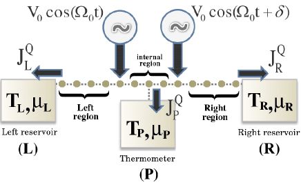
Figure 1: Scheme of the set up. The central device is a wire connected to the left and right. The third reservoir ($P$) represents the thermometer, which consists of a macroscopic system weakly coupled to a given point of the central device.

We consider here the same set-up as in Ref. cal, which we display in Fig. 1. This is a quantum driven system described by a Hamiltonian $H_{sys}(t)$ and a thermometer characterized by a Hamiltonian $H_{P}$ that are locally coupled via $H_{cP}$ in such a way that the total Hamiltonian can be written as

$$H(t)=H_{sys}(t)+H_{cP}+H_{P}.$$ (1)

For the driven system we take a device composed of a central part [$H_{C}(t)$] and two reservoirs ($H_{L},H_{R}$), coupled to the central part via contacts ($H_{cL},H_{cR}$),

$$H_{sys}(t)=H_{L}+H_{cL}+H_{C}(t)+H_{cR}+H_{R}.$$ (2)

The Hamiltonian describing the central system ($C$) contains the ac driving fields, $H_{C}(t)=H_{0}+H_{V}(t)$. We assume that $H_{0}$ is a Hamiltonian for non interacting electrons while $H_{V}(t)$ is harmonically time dependent, i.e., $H_{V}(t)=\sum_{n=-\infty}^{+\infty}e^{-i\Omega_{0}nt}H_{V}(n)$. We leave further details of the model for the moment undetermined in order to make the coming discussion as model independent as possible.

Both reservoirs and the local probe are modeled by systems of non interacting electrons with many degrees of freedom: $H_{\alpha}=\sum_{k\alpha}\varepsilon_{k\alpha}c^{\dagger}_{k\alpha}c_{k\alpha}$, where $\alpha=L,R,P$. The corresponding contacts are $H_{c\alpha}=w_{c\alpha}(c^{\dagger}_{k\alpha}c_{l\alpha}+c^{\dagger}_{l\alpha}c_{k\alpha})$, where $l\alpha$ denotes the coordinate of $C$ at which the reservoir $\alpha$ is connected. As in previous works,cal ; fourpoint ; fourpointfed we consider a non invasive probe, which implies that $w_{cP}$ is small enough to be treated at the lowest order of perturbation theory when necessary.

To describe the dynamics of the system we use the Schwinger-Keldysh-Green functions formalism. This involves the calculation of the Keldysh and retarded Green functions,

$$G^{K}_{l,l^{\prime}}(t,t^{\prime}) = i\langle c^{\dagger}_{l^{\prime}}(t^{\prime})c_{l}(t)-c_{l}(t)c^{\dagger}_{l^{\prime}}(t^{\prime})\rangle,$$

$$G^{R}_{l,l^{\prime}}(t,t^{\prime}) = -i\Theta(t-t^{\prime})\langle c_{l}(t)c^{\dagger}_{l^{\prime}}(t^{\prime})+c^{\dagger}_{l^{\prime}}(t^{\prime})c_{l}(t)\rangle,$$ (3)

where the indexes $l,l^{\prime}$ denote spatial coordinates of the central system. These Green functions can be evaluated after solving the Dyson equations. For the case of harmonic driving it is convenient to use the Floquet-Fourier representation of the Green functions: liliflo

$$G_{l,l^{\prime}}^{K,R}(t,t-\tau)=\sum_{k=-\infty}^{\infty}\int_{-\infty}^{\infty}\frac{d\omega}{2\pi}e^{-i(k\Omega_{0}t+\omega\tau)}G_{l,l^{\prime}}^{K,R}(k,\omega).$$ (4)

III Defining the temperature

III.1 Local temperature determined by a thermometer

Heat transport through the central system can occur due to a temperature or chemical potential difference between the reservoirs as well as as the result of pumping by the external sources. In a generic situation, if the probe is connected to the central system, there is also heat exchange between the system and the probe. In Ref. cal, the local temperature $T_{lP}$ was defined as the value of $T_{P}$ (i.e., the temperature of the probe) such that heat exchange between the central system and the probe vanishes.

It can be shownliliheatpump that, given $H_{C}(t)$ without many-body interactions, the heat current from the central system and the thermometer can be expressed as ($\hbar=k_{B}=e=1$)

$$J_{P}^{Q}=\sum_{\alpha=L,R,P}\sum_{k=-\infty}^{\infty}\int_{-\infty}^{\infty}\frac{d\omega}{2\pi}\{[f_{\alpha}(\omega)-f_{P}(\omega_{k})]$$

$$\times(\omega_{k}-\mu)\Gamma_{P}(\omega_{k})\Gamma_{\alpha}(\omega)\left|G^{R}_{lP,l\alpha}(k,\omega)\right|^{2}\},$$ (5)

where $\omega_{k}=\omega+k\Omega_{0}$ and $\Gamma_{\alpha}(\omega)=-2\pi|w_{\alpha}|^{2}\sum_{k\alpha}\delta(\omega-\varepsilon_{k\alpha})$ are the spectral functions that determine the escape to the reservoirs ($\alpha=L,R,P$), and $f_{\alpha}(\omega)=1/[e^{\beta_{\alpha}(\omega-\mu_{\alpha})}+1]$ is the Fermi function, which depends on $T_{\alpha}=1/\beta_{\alpha}$ and $\mu_{\alpha}$ the temperature and the chemical potential of the reservoir $\alpha$. Thus, the local temperature $T_{lP}$ corresponds to the solution of the equation

$$J_{P}^{Q}(T_{lP})=0.$$ (6)

In Ref. cal, the value of $\mu_{P}$ was kept fixed (and equal to that of the reservoirs, $\mu_{L}=\mu_{R}=\mu_{P}$). Our thermometer, however, is a reservoir not only for energy but also for particles. In fact, the same setup but with the role of temperature and chemical potential exchanged was considered in Refs. fourpoint, and fourpointfed, to define the local voltage of a driven structure. One question that arises is how the situation gets modified when we allow both the temperature and the voltage of the probe to adjust simultaneously to define the local temperature and the local voltage. Such a procedure has been followed in Ref. polianski, . Thus, in an analogous way as we did before, we now define the local temperature $T_{lP}^{*}$ (where we use the $*$ symbol to distinguish it from the definition above) and local voltage $\mu_{lP}^{*}$, respectively, as the temperature and the voltage of the probe that vanish simultaneously both the charge and the heat currents between the system and the probe, i.e.,

$$\left\{\begin{array}[]{rcl}J^{Q}_{P}(T_{P}^{*},\mu_{P}^{*})&=&0,\\ J^{e}_{P}(T_{P}^{*},\mu_{P}^{*})&=&0,\end{array}\right.$$

where (see Refs. liliflo, ; fourpointfed, )

$$J_{P}^{e}=\sum_{\alpha=L,R,P}\sum_{k=-\infty}^{\infty}\int_{-\infty}^{\infty}\frac{d\omega}{2\pi}\{[f_{\alpha}(\omega)-f_{P}(\omega_{k})]$$

$$\times\Gamma_{P}(\omega_{k})\Gamma_{\alpha}(\omega)\left|G^{R}_{lP,l\alpha}(k,\omega)\right|^{2}\}.$$ (7)

III.2 Effective temperature from a Fluctuation-Dissipation Relation

For systems in equilibrium, the fluctuation dissipation theorem establishes a relation between the Keldysh (correlation) and retarded Green functions. Indeed, for a system like the one under consideration, but without the time-dependent fields, it can be shown that the relation between the fluctuations in the system, $iG_{l,l}^{0,K}(\omega)$, with the dissipation term of the bath, $\Gamma_{\alpha}(\omega)$, is letogus ; lilileto

$$iG_{l,l}^{0,K}(\omega)=\tanh[\frac{\beta(\omega-\mu)}{2}]\varphi^{0}_{l}(\omega),$$ (8)

$$\varphi^{0}_{l}(\omega)=-2\mbox{Im}[G_{l,l}^{0,R}(\omega)]=\sum_{\alpha=L,R}|G^{0,R}_{l,l\alpha}(\omega)|^{2}\Gamma_{\alpha}(\omega),$$ (9)

where the index ⁰ indicates that we are considering the equilibrium system, i.e. with the term $H_{V}(t)=0$ and all the reservoirs at the same temperature $T=1/\beta$.

In the presence of time-dependent voltages it can be shown that

$$iG^{K}_{l,l}(0,\omega) = \sum_{k=-\infty}^{\infty}\tanh[\frac{\beta(\omega_{-k}-\mu)}{2}]\varphi_{l}(k,\omega_{-k}),$$ (10)

$$\varphi_{l}(k,\omega) = \sum_{\alpha=L,R}\left|G^{R}_{l,l\alpha}(k,\omega)\right|^{2}\Gamma_{\alpha}(\omega).$$ (11)

In Ref. cal, we have shown that within the weak driving-adiabatic regime, where the term $H_{V}(t)$ is treated as a perturbation and the driving frequency is smaller than the dwell time of the electrons within the central system adia , it is possible to define an effective temperature $T^{eff}_{l}=1/\beta^{eff}_{l}$ through the following relation:

$$iG^{K}_{l,l}(0,\omega)-iG^{K}_{l,l}(0,\mu) = \tanh[\frac{\beta^{eff}_{l}(\omega-\mu)}{2}]\overline{\varphi_{l}}(\omega),$$ (12)

with $\overline{\varphi_{l}}(\omega)=-2\mbox{Im}[G_{l,l}^{R}(0,\omega)]=\sum_{k}\varphi_{l}(k,\omega_{-k})$. A similar relation in the time domain has been studied numerically for a driven ring in contact with a reservoir. lilileto

IV Results

In this section we present results for a central device consisting of non-interacting electrons in a one-dimensional lattice:

$$H_{0}=-w\sum_{l,l^{\prime}}(c^{\dagger}_{l}c_{l^{\prime}}+h.c.),$$ (13)

where $w$ denotes a hopping matrix element between neighboring positions $l,l^{\prime}$ on the lattice, and a driving term of the form:

$$H_{V}(t)=\sum_{j=1}^{2}eV_{j}(t)c^{\dagger}_{lj}c_{lj},$$ (14)

with $V_{j}(t)=V_{0}\cos(\Omega_{0}t+\delta_{j})$, $lj$ being the positions at where two ac fields oscillating with the same frequency and a phase-lag are applied. This defines a simple model for a quantum pump where two ac gate voltages are applied at the walls of a quantum dot. liliflo ; adia ; pump

IV.1 Equivalence between the different definitions of the temperature at weak driving

In Ref. cal, we have analyzed the weak driving, which corresponds to the ac voltage amplitudes lower than the kinetic energy of the electrons in the structure and the driving frequency lower than the inverse of the dwell time of these electrons. We have analytically shown in this case that the local temperature defined from Eq. (6), with the chemical potential of the reservoir kept fixed, is identical to the effective temperature defined from the local fluctuation-dissipation relation given by Eq. (12). That is,

$$T^{eff}_{lP}=T_{lP}.$$ (15)

In Sec. A.1 of the Appendix we summarize the main steps leading to this result and we also show that within the weak-driving regime the local temperature can be expressed as

$$T_{lP}^{2} \sim T^{2}+\frac{3}{\pi^{2}}\lambda_{lP}^{(0)}(\mu)\Omega_{0}^{2}+2\lambda_{lP}^{(1)}(\mu)T^{2}\Omega_{0}$$ (16)

$$-\frac{1}{2}\lambda_{lP}^{(2)}(\mu)T^{2}\Omega_{0}^{2},$$

with

$$\lambda_{l}^{(n)}(\omega)=\frac{1}{\sum_{k=-1}^{1}\varphi_{l}(k,\omega)}\sum_{k=-1}^{1}(k)^{n+2}\frac{d^{n}[\varphi_{l}(k,\omega)]}{d\omega^{n}},$$ (17)

$$\varphi_{l}(k,\omega)=\sum_{\alpha=L,R}\left|G^{R}_{l,l\alpha}(k,\omega)\right|^{2}\Gamma_{\alpha}(\omega).$$ (18)

By keeping only the lowest order in $\Omega_{0}$, the local temperature $T_{lP}$ can be cast into the form

$$T_{lP}=T\left[1+\lambda^{(1)}_{lP}(\mu)\Omega_{0}\right].$$ (19)

Analytical expressions for $T_{lP}^{*}$ defined in Eqs. (III.1) are considerable harder to obtain than those $T_{lP}$. Nevertheless, we have been able to show that within the regime of interest (see Sec. A.2 of the Appendix for details)

$$T_{lP}^{*}=T\left[1+\Omega_{0}\frac{d}{d\omega}\left(\frac{\sum_{k=-1}^{1}k\varphi_{lP}(k,\omega)}{\sum_{k=-1}^{1}\varphi_{lP}(k,\omega)}\right)_{\omega=\mu}\right].$$ (20)

It is easy to see that for $\left.\frac{d}{d\omega}\Gamma_{\alpha}\right|_{\omega=\mu}\sim 0$, which is in general satisfied for metallic electrodes with a featureless band, Eq. (20) becomes

$$T_{lP}^{*}=T\left[1+\lambda^{(1)}_{lP}(\mu)\Omega_{0}\right]=T_{lP}.$$ (21)

Thus, it is possible to prove that all the three definitions of the local temperature, $T_{eff}$ from a fluctuation-dissipation relation, $T_{lP}$ from a thermometer, and $T^{*}_{lP}$ from a thermometer that is also a voltage probe, coincide within the weak-driving regime.

IV.2 Temperature and the direction for heat flow

We now turn to explore the relation between the local temperature and heat flow between the central system and the left and right reservoirs.

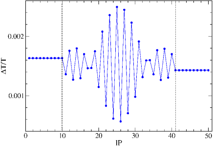
Figure 2: (Color online) Local temperature along a one-dimensional model of $N=50$ sites with two ac fields operating with a phase lag of $\delta=\pi/2$ at the positions indicated by dotted lines. The system is in contact with reservoirs with chemical potentials $\mu=0.2$ and temperature $T=0.025$. The driving frequency is $\Omega_{0}=0.05$ and the amplitude is $V_{0}=0.05$.

In Fig. 2 we show a typical temperature profile along the structure. The value of $T_{l}$ is plotted for each point of the chain, for $T_{L}=T_{R}=T$, $\mu_{L}=\mu_{R}=\mu$, and a particular low value $\Omega_{0}$. We can distinguish two regions within the central structure, denoted as “Left” and “Right” regions in Fig. 1, which are defined between the contact with the left (right) reservoir and the left (right) pumping centers. The local temperature at weak driving is constant within these regions but different from the one of the reservoirs. In the internal region between the two pumping centers, the local temperature displays $2k_{F}$ Friedel-like oscillations, $k_{F}$ being the Fermi vector of the electrons leaving the reservoirs. This feature is similar to the one observed in other small size structures under stationary driving dubi-diventra and has the same origin as the oscillations in the local voltage profile sensed by a voltage probe, fourpoint ; fourpointfed namely, the interference generated by elastic scattering processes at the two pumping centers.

We would like to explore whether heat flow through the contacts to the reservoirs is described by a relation of the type

$$J^{Q}_{\alpha}=K_{\alpha}\Delta T_{\alpha},$$ (22)

as it happens in systems where the heat flow is induced by an explicit temperature gradient. In our case, the gradient is defined as $\Delta T_{\alpha}=T_{l\alpha}-T_{\alpha}$, $T_{l\alpha}$ being the local temperature at the point of the central device connected to the $\alpha$ reservoir, while $K_{\alpha}$ is a positive effective contact thermal conductance. Thus, we evaluate independently the dc components of the heat currents between the system and each of the reservoirs, as well as the local temperatures at the contacts. Results for heat flow and local temperature gradients $\Delta T_{\alpha}$ are shown in Fig. 3, as functions of the pumping frequency for reservoirs with the same temperature $T$ and the same chemical potential $\mu$. Since the dc heat current is $\propto V_{0}^{2}$ for low driving amplitudes, we found it convenient to show $J^{Q}/V_{0}^{2}$ in the figure. The flow is defined as positive (negative) when the heat flows to (from) the reservoir.

The behavior of the heat flow at the left reservoir ($L$) corresponds to a situation in which heat enters the reservoir. This is associated with the idea of heat flowing from a hot region to a colder one. Correspondingly, the local temperature at the contact point of the system is higher than $T_{L}$.

Nevertheless, in a pumping regime, we expect to find situations in which heat can be extracted from one reservoir to be pumped into the system and the other reservoir. This is indeed the situation for the right lead ($R$), where for very low frequencies the heat flow is negative. In the same figure we show that the corresponding gradient of temperature along the contact shows a behavior compatible with the heat flow. That is, $T_{lR}$ is lower than $T_{R}$.

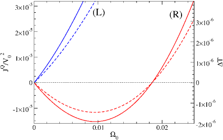
Figure 3: (Color online) dc heat current divided by $V_{0}^{2}$ (solid) and local temperature difference (dashed) between the system and the left reservoir (blue) or the right reservoir (red) as a function of driving frequency $\Omega_{0}$. The phase lag is $\delta=1.88$ and the driving amplitude is $V_{0}=0.05$. The temperature and the chemical potential of the reservoirs are $T=0.025$ and $\mu=0.2$.

For higher frequencies, the heat flows into the two reservoirs. This is the most common situation, where the central system becomes heated by the driving voltage and the generated heat is dissipated into the reservoirs. In this regime, the behavior of the gradient of temperature along the contact also exactly follows the direction of the heat flow. In particular, notice in the figure that both $J^{Q}_{R}$ and $\Delta T_{R}$ change the sign exactly at the same frequency.

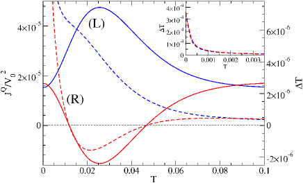
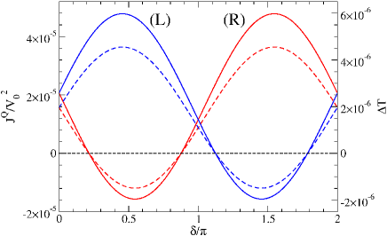
Figure 4: (Color online) Upper panel: Heat flow (solid) and local temperature difference (dashed) between the system and the left reservoir (blue) or the right reservoir (red) as a function of the temperature $T$ of the reservoirs. The phase lag is $\delta=\pi/2$, the driving frequency is $\Omega_{0}=0.01$ and the amplitude is $V_{0}=0.05$. The chemical potential of the reservoirs is $\mu=0.2$. Lower panel: Heat flow (solid) and local temperature difference (dashed) between the system and the left reservoir (blue) or the right reservoir (red) as a function of the phase lag. The driving frequency is $\Omega_{0}=0.01$ and the amplitude is $V_{0}=0.05$. The temperature and the chemical potential of the reservoirs are $T=0.025$ and $\mu=0.2$.

The existence of the pumping regime, requires a delicate interplay between pumping frequency, temperature, and phase lag but in all cases we found that the behavior of $\Delta T_{\alpha}$ agrees with that expected from considerations of heat flow. In Fig. 4 we show the heat flow as a function of $T$ and as a function of phase lag $\delta$. As expected from the symmetries of the set-up, a change of phase $\delta\rightarrow 2\pi-\delta$ enforces $L\rightarrow R$. In all the cases, the behavior of the heat flow is in complete agreement with Eq. (22).

IV.3 Generalized Wiedemann-Franz law

Another interesting property which points toward the identification of $T_{l\alpha}$ with a bona fide temperature concerns a generalization of the Wiedemann-Franz law which we discuss next. In addition to the thermal conductance defined above, we can consider the voltage probes as in Refs. fourpoint, ; fourpointfed, to calculate the local voltage at the contact and define the effective electrical contact conductance as follows:

$$G_{\alpha}=\frac{J^{e}_{\alpha}}{\Delta\mu_{\alpha}},$$ (23)

where

$$\Delta\mu_{\alpha}=\mu_{\alpha}-\mu_{l{\alpha}},$$ (24)

where $\mu_{\alpha}$ is the chemical potential of reservoir $\alpha$ and $\mu_{l\alpha}$ is the local chemical potential of the central system site connected to reservoir $\alpha$. As in the previous section we consider $T_{\alpha}=T$ and $\mu_{\alpha}=\mu$ for $\alpha=L,R$.

In order to calculate $K_{\alpha}$ we need the heat current $J^{Q}_{\alpha}$ that flows into the reservoir $\alpha$ and $\Delta T_{\alpha}$. We focus on the weak-driving regime. For non invasive thermometers, the heat current that flows into the reservoir $\alpha$ is

$$J^{Q}_{\alpha}=\sum_{k}\int\frac{d\omega}{2\pi}(f(\omega)-f(\omega_{k}))(\omega_{k}-\mu)\tilde{\varphi}_{\alpha}(k,\omega),$$ (25)

where

$$\tilde{\varphi}_{\alpha}(k,\omega)=\sum_{\beta=L,R}\Gamma_{\alpha}(\omega_{k})\left|G^{R}_{l\alpha,l\beta}(k,\omega)\right|^{2}\Gamma_{\beta}(\omega).$$ (26)

If the temperature $T$ of the reservoirs is small compared to their Fermi energy, we can apply the Sommerfeld expansion up to order $T^{2}$. The low-driving-frequency assumption is introduced by expanding all the terms of Eq. (25) in powers of $\Omega_{0}$. Under these conditions, the heat current can be rewritten as follows:

$$J^{Q}_{\alpha} = \frac{1}{4\pi}\sum_{k}\left\{k^{2}\Omega_{0}^{2}\tilde{\varphi}_{\alpha}(k,\mu)+T^{2}\frac{\pi^{2}}{3}\left[2\frac{d\tilde{\varphi}_{\alpha}}{d\omega}(k,\mu)\right.\right.$$ (27)

$$-\left.\left.\frac{1}{2}\frac{d^{2}\tilde{\varphi}_{\alpha}}{d\omega^{2}}(k,\mu)k\Omega_{0}\right]k\Omega_{0}\right\}.$$

For high temperature compared to the driving ($T\gg\Omega_{0}$), $J^{Q}_{\alpha}$ and $\Delta T_{\alpha}$ [see Eqs. (21) and (27)] are

$$J^{Q}_{\alpha} = T^{2}\frac{\pi}{6}\sum_{k}k\frac{d\tilde{\varphi}_{\alpha}}{d\omega}(k,\mu)\Omega_{0},$$ (28)

$$\Delta T_{\alpha} = T\lambda^{(1)}_{l\alpha}(\mu)\Omega_{0}.$$ (29)

Using the definitions of $\tilde{\varphi}_{\alpha}$ and $\lambda^{(1)}_{l}$ given in Eqs. (26) and (17), respectively, it is easy to show that the thermal conductance is

$$K_{\alpha}=\frac{\pi}{6}\tilde{\varphi}_{\alpha}(\mu)T,$$ (30)

where

$$\tilde{\varphi}_{\alpha}(\mu)=\sum_{k}\tilde{\varphi}_{\alpha}(k,\mu).$$ (31)

The electrical conductance can be calculated in an analogous way. Applying the Sommerfeld expansion, expanding all the terms in powers of $\Omega_{0}$, and keeping up to first order, the charge current that flows into reservoir $\alpha$ can be written in the following way:

$$J^{e}_{\alpha}=\frac{1}{2\pi}\sum_{k}k\tilde{\varphi}_{\alpha}(k,\mu)\Omega_{0}.$$ (32)

For $\Delta\mu_{\alpha}$, the expression is [see Eq. (77)]

$$\Delta\mu_{\alpha}=\frac{\sum_{k}k\varphi_{l\alpha}(k,\mu)}{\sum_{k}\varphi_{l\alpha}(k,\mu)}\Omega_{0}.$$ (33)

Hence, the electrical conductance $G_{\alpha}$ is

$$G_{\alpha}=\frac{1}{2\pi}\tilde{\varphi}_{\alpha}(\mu).$$ (34)

It is possible to show that this result for the electrical conductance is actually valid for all temperatures.

At this point it may be convenient to restate units in order to make it easier to extract useful information from this result. Then, from Eqs. (30) and (34) it follows that for the weak-driving regime, where $T\gg\Omega_{0}$, the thermal and electrical conductances satisfy the Wiedemann-Franz law

$$\frac{K_{\alpha}}{G_{\alpha}}=\frac{\pi^{2}}{3}\left(\frac{k_{B}}{e}\right)^{2}T.$$ (35)

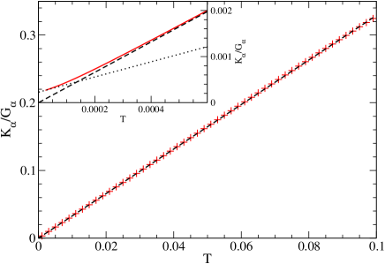
Figure 5: (Color online) $K/G$ for the right contact (red crosses) as a function of temperature. The black dashed line represents the Wiedemann-Franz law. Inset: The black dotted line represents the behavior of the quotient $K/G$ (red line) for very low temperatures, as depicted in Eq. (39). The phase-lag is $\delta=\pi/2$, the driving frequency is $\Omega_{0}=0.005$ and the amplitude is $V_{0}=0.05$. The chemical potential of the reservoirs is $\mu=0.2$.

In Fig. 5 we show the ratio $K_{\alpha}/G_{\alpha}$ for $\alpha=R$ as a function of temperature $T$. The curve for the left reservoir is identical and it is not shown. We see that for very low $T$, the Wiedemann-Franz law is not satisfied. In the low-temperature regime where $T\ll\Omega_{0}$, from Eqs. (27) and (77) it follows that $J^{Q}_{\alpha}$ and $\Delta T_{\alpha}$ can be written as

$$J^{Q}_{\alpha} = \frac{1}{4\pi}\sum_{k}k^{2}\Omega_{0}^{2}\tilde{\varphi}_{\alpha}(k,\mu),$$ (36)

$$\Delta T_{\alpha} = \sqrt{\frac{3}{\pi^{2}}\lambda^{(0)}_{l\alpha}(\mu)}\Omega_{0}-T.$$ (37)

Hence, the effective thermal conductance $K_{\alpha}$ is

$$K_{\alpha}=\frac{1}{4\sqrt{3}}\frac{\sum_{k}k^{2}\tilde{\varphi}_{\alpha}(k,\mu)}{\sqrt{\lambda^{(0)}_{l\alpha}(\mu)}}\Omega_{0}+\frac{\pi}{12}\tilde{\varphi}_{\alpha}(\mu)T.$$ (38)

In this equation it is important to remark that the thermal conductance is finite even when the temperature $T$ of the reservoirs equals zero.

From Eqs. (34) and (38) it follows that for low temperature the quotient $K_{\alpha}/G_{\alpha}$, to the lowest order in $\Omega_{0}$ and $T$, is

$$\frac{K_{\alpha}}{G_{\alpha}}=\frac{\pi}{2\sqrt{3}}\sqrt{\tilde{\lambda}^{(0)}_{\alpha}(\mu)}\ \Omega_{0}+\frac{\pi^{2}}{6}T,$$ (39)

where

$$\tilde{\lambda}^{(0)}_{\alpha}(\omega)=\frac{1}{\sum_{k}\tilde{\varphi}_{\alpha}(k,\omega)}{\sum_{k}k^{2}\tilde{\varphi}_{\alpha}(k,\omega)}.$$ (40)

Using the value of $\Delta T_{\alpha}$ for $T=0$ given in Eq. (77) we can rewrite Eq. (39), with units restated as

$$\frac{K_{\alpha}}{G_{\alpha}}=\frac{\pi^{2}}{6}\left(\frac{k_{B}}{e}\right)^{2}\left[\Delta T_{\alpha}|_{T=0}+T\right].$$ (41)

From this equation we can see that as the temperature $T$ of the reservoirs goes to zero, the quotient $K_{\alpha}/G_{\alpha}$ approaches linearly a finite value, explaining the behavior observed in Fig. 5.

V Summary and Conclusions

In this work we have analyzed the relation between different definitions of temperature in a nonequilibrium setup and its physical meaning, mainly in connection with heat flow. More specifically, we have generalized the definition of local temperature introduced in Ref. cal, to allow for the thermometer to act also as a voltage probe and we have shown that in the situation of interest, i.e, weak driving (small deviations from equilibrium) and weak system-thermometer coupling (i.e., noninvasive probe), both definitions coincide, and consequently, both definitions give the same value as the effective temperature introduced by the fluctuation-dissipation relation.

We have also shown that within the low-driving regime, it is possible to define an effective contact thermal conductance as the quotient between the dc heat current flowing through a given contact to a reservoir and the effective temperature gradient defined as the difference between the local temperature at the contact point of the system and the temperature of the reservoir. The behavior of such an effective temperature gradient exactly follows the direction of the heat flow between the system and the reservoirs. This is consistent with the idea that the local temperature at the contact does behave as a bona fide temperature.

*

Appendix A Analytical expression for local temperature

A.1 Local temperature determined with fixed chemical potential of the thermometer

In this section we present the detailed calculation of the local temperature, within the adiabatic, low-temperature, and weak-driving regimes.

In the weak-driving regime we only keep the terms up to order $(V_{0})^{2}$ (i.e., Floquet-Fourier components with $k=-1,0,1$). Treating the coupling to the thermometer $w_{cP}$ at the lowest order in perturbation theory and considering that the spectral function of the thermometer $\Gamma_{P}(\omega)$ is roughly constant, the heat current that flows into the thermometer can be written as follows:

$$J_{P}^{Q}\propto\sum_{k=-1}^{1}\int d\omega\phi_{lP}^{Q}(k,\omega)\left[f(\omega)-f_{P}(\omega_{k})\right],$$ (42)

where

$$\phi_{l}^{Q}(k,\omega)=(\omega_{k}-\mu)\varphi_{l}(k,\omega),$$ (43)

$$\varphi_{l}(k,\omega)=\sum_{\alpha=L,R}\left|G^{R}_{l,l\alpha}(k,\omega)\right|^{2}\Gamma_{\alpha}(\omega).$$ (44)

If the temperature $T$ of the reservoirs is small compared to their Fermi energy, we can apply the Sommerfeld expansion up to order $T^{2}$. Under this condition the heat current can be rewritten as

$$J_{P}^{Q} \propto \sum_{k=-1}^{1}\left\{\int_{\mu-k\Omega_{0}}^{\mu}d\omega\phi_{lP}^{Q}(k,\omega)+\frac{\pi^{2}}{6}T^{2}F_{lP}^{Q}(k,\mu)\right.$$ (45)

$$-\left.\frac{\pi^{2}}{6}(T_{lP})^{2}F_{lP}^{Q}(k,\mu-k\Omega_{0})\right\},$$

where

$$F_{l}^{Q}(k,\omega)=\frac{d}{d\omega}\phi_{l}^{Q}(\omega).$$ (46)

The local temperature $T_{lP}$ corresponds to the solution of the equation $J^{Q}_{P}(T_{lP})=0$. Directly from the expression for the heat current given in Eq.(45) we can obtain $T_{lP}$:

$$(T_{lP})^{2}\sim\frac{\frac{6}{\pi^{2}}\sum_{k}\Phi_{lP}(k)+T^{2}\sum_{k}F_{lP}^{Q}(k,\mu)}{\sum_{k}F_{lP}^{Q}(k,\mu-k\Omega_{0})},$$ (47)

where

$$\Phi_{l}(k)=\int_{\mu-k\Omega_{0}}^{\mu}d\omega\phi_{l}^{Q}(k,\omega).$$ (48)

The adiabatic condition is introduced by expanding all the terms of Eq. (47) in powers of the driving frequency $\Omega_{0}$. It is easy to show that the first term of the numerator is of second order in $\Omega_{0}$:

$$\sum_{k=-1}^{1}\Phi_{lP}(k)\approx\frac{1}{2}\Omega_{0}^{2}\sum_{k=-1}^{1}k\,\varphi_{lP}(k,\mu).$$ (49)

The second term of the numerator of Eq. (47) is

$$\sum_{k=-1}^{1}F_{lP}(k,\mu)=\sum_{k=-1}^{1}\left[\varphi_{lP}(k,\mu)+k\Omega_{0}\frac{d\varphi_{lP}}{d\omega}(k,\mu)\right].$$ (50)

Expanding the denominator of Eq. (47) up to second order in $\Omega_{0}$ we obtain

$$\sum_{k=-1}^{1}F_{lP}^{Q}(k,\mu-k\Omega_{0}) \approx \sum_{k=-1}^{1}\left[\varphi_{lP}(k,\mu)-k\frac{d\varphi_{lP}}{d\omega}(k,\mu)\Omega_{0}\right.$$ (51)

$$\left.+\frac{1}{2}k^{2}\frac{d^{2}\varphi_{lP}}{d\omega^{2}}(k,\mu)\Omega_{0}^{2}\right].$$

Thus, keeping up to second order in $\Omega_{0}$ in Eq. (47) for the local temperature we obtain

$$(T_{lP})^{2} \sim \frac{3}{\pi^{2}}\lambda_{lP}^{(0)}(\mu)\Omega_{0}^{2}+T^{2}\left(1+\right.$$ (52)

$$\left.2\lambda_{lP}^{(1)}(\mu)\Omega_{0}-\frac{1}{2}\lambda_{lP}^{(2)}(\mu)\Omega_{0}^{2}\right),$$

where

$$\lambda_{l}^{(n)}(\omega)=\frac{1}{\sum_{k=-1}^{1}\varphi_{l}(k,\omega)}\sum_{k=-1}^{1}(k)^{n+2}\frac{d^{n}[\varphi_{l}(k,\omega)]}{d\omega^{n}},$$ (53)

and $\varphi_{l}(k,\omega)$ is given in Eq. (44).

In particular, for the case of finite temperature $T$ of the reservoirs, and high temperature compared to the driving ($T\gg\Omega_{0}$), Eq. (52) reduces to

$$T_{lP}=T\left[1+\lambda_{lP}^{(1)}(\mu)\Omega_{0}\right].$$ (54)

For the case of reservoirs at very low temperature ($T\ll\Omega_{0}$), Eq. (52) leads to

$$\Delta T_{lP}=\sqrt{\frac{3}{\pi^{2}}\lambda_{lP}^{(0)}(\mu)}\Omega_{0}-T.$$ (55)

A.2 Local temperature determined simultaneously with local chemical potential of the thermometer

An alternative definition of local temperature to the one given in Sec. A.1 is the following: the local temperature $T_{lP}^{*}$ and the local chemical potential $\mu_{lP}^{*}$ are the values of the temperature and the chemical potential of the probe that vanish simultaneously $J^{Q}_{P}$ and $J^{e}_{P}$:

$$\left\{\begin{array}[]{rcl}J^{Q}_{P}(T_{lP}^{*},\mu_{lP}^{*})&=&0,\\ J^{e}_{P}(T_{lP}^{*},\mu_{lP}^{*})&=&0.\end{array}\right.$$

As we did in Sec. A.1 we only keep terms up to order $(V_{0})^{2}$ for the weak-driving regime. Treating the coupling to the thermometer $w_{cP}$ at the lowest order in perturbation theory and considering that the spectral function of the thermometer $\Gamma_{P}(\omega)$ is roughly constant, the energy and charge currents that flow into the thermometer can be written as follows:

$$J_{P}^{X}\propto\sum_{k=-1}^{1}\int d\omega\phi_{lP}^{X}(k,\omega)\left[f(\omega)-f_{P}(\omega_{k})\right],$$ (56)

where $X=Q,e$ and

$$\phi_{l}^{Q}(k,\omega)=(w_{k}-\mu_{P})\varphi_{l}(k,\omega),$$ (57)

$$\phi_{l}^{e}(k,\omega)=\varphi_{l}(k,\omega),$$ (58)

where $\varphi_{l}(k,\omega)$ is given in Eq. (44).

Applying the Sommerfeld expansion up to order $T^{2}$ and defining $\mu_{lP}^{*}\equiv\mu+\Delta\mu_{lP}^{*}$, Eq. (56) can be rewritten as

$$J_{P}^{X} \propto \sum_{k=-1}^{1}\left\{\int_{\mu_{-}k\Omega_{0}+\Delta\mu_{lP}^{*}}^{\mu}d\omega\phi_{lP}^{X}(k,\omega)+\frac{\pi^{2}}{6}T^{2}F_{lP}^{X}(k,\mu)\right.$$ (59)

$$-\left.\frac{\pi^{2}}{6}(T_{lP}^{*})^{2}F_{lP}^{X}(k,\mu-k\Omega_{0}+\Delta\mu_{lP}^{*})\right\},$$

where

$$F_{l}^{X}(k,\omega)=\frac{d}{d\omega}\phi_{l}^{X}(\omega).$$ (60)

We expect $\Delta\mu_{lP}^{*}$ to be at least of order $\Omega_{0}$. We expand the first term of Eq. (59) up to second order in $\Omega_{0}$:

$$\int_{\mu-k\Omega_{0}+\Delta\mu_{lP}^{*}}^{\mu}d\omega\phi_{lP}^{X}(k,\omega) = -\phi_{lP}^{X}(k,\mu)(\Delta\mu_{lP}^{*}-k\Omega_{0})$$

$$-\frac{1}{2}F_{lP}^{X}(k,\mu)(\Delta\mu_{lP}^{*}-k\Omega_{0})^{2}.$$

In the case of finite temperature $T$ of the reservoirs, we define $T_{lP}^{*}\equiv T+\Delta T_{lP}^{*}$ and expect $\Delta T_{lP}^{*}$ to be at least of order $\Omega_{0}$. Hence, to the lowest order in $\Omega_{0}$, $J^{e}$ and $J^{Q}$ become

$$\left\{\begin{array}[]{rcl}J^{e}_{P}(T_{lP}^{*},\mu_{lP}^{*})&\propto&-a\Delta\mu_{lP}^{*}-b\Delta T_{lP}^{*}+\alpha\Omega_{0},\\ J^{Q}_{P}(T_{lP}^{*},\mu_{lP}^{*})&\propto&-c\Delta\mu_{lP}^{*}-d\Delta T_{lP}^{*}+\beta\Omega_{0},\end{array}\right.$$ (62)

where

$$a = \sum_{k=-1}^{1}\left[\varphi_{lP}(k,\mu)+\frac{\pi^{2}}{6}T^{2}\frac{d^{2}\varphi_{lP}}{d\omega^{2}}(k,\mu)\right],$$ (63)

$$b = \frac{\pi^{2}}{3}T\sum_{k=-1}^{1}\frac{d\varphi_{lP}}{d\omega}(k,\mu),$$ (64)

$$c = T\sum_{k=-1}^{1}\frac{d\varphi_{lP}}{d\omega}(k,\mu),$$ (65)

$$d = \sum_{k=-1}^{1}\varphi_{lP}(k,\mu),$$ (66)

$$\alpha = \sum_{k=-1}^{1}k\left[\varphi_{lP}(k,\mu)+\frac{\pi^{2}}{6}T^{2}\frac{d^{2}\varphi_{lP}}{d\omega^{2}}(k,\mu)\right],$$ (67)

$$\beta = T\sum_{k=-1}^{1}k\frac{d\varphi}{d\omega}(k,\mu).$$ (68)

Within the approximations, the solution of the equations given in Eq. (A.2) is

$$\left\{\begin{array}[]{rcl}\Delta\mu_{lP}^{*}&=&\frac{1}{\Delta}(d\alpha-b\beta)\Omega_{0},\\ \\ \Delta T_{lP}^{*}&=&\frac{1}{\Delta}(a\beta-c\alpha)\Omega_{0},\end{array}\right.$$ (69)

where

$$\Delta=ad-bc=\left(\sum_{k}\varphi_{lP}(k,\mu)\right)^{2}+O(T)^{2}.$$ (70)

Hence,

$$\left\{\begin{array}[]{rcl}\Delta\mu_{lP}^{*}&=&\left(\frac{\sum_{k}k\varphi_{lP}(k,\mu)}{\sum_{k}\varphi_{lP}(k,\mu)}+O(T)^{2}\right)\Omega_{0},\\ \\ \Delta T_{lP}^{*}&=&T\left[\frac{d}{d\omega}\left(\frac{\sum_{k}k\varphi_{lP}(k,\omega)}{\sum_{k}\varphi_{lP}(k,\omega)}\right)_{\omega=\mu}+O(T)^{2}\right]\Omega_{0}.\end{array}\right.$$ (71)

Considering that $\left.\frac{d}{d\omega}\Gamma_{\alpha}\right(\omega)|_{\omega=\mu}\sim 0$, then $T_{lP}^{*}$ becomes

$$T_{lP}^{*}=T\left[1+\lambda^{(1)}_{lP}(\mu)\Omega_{0}\right],$$ (72)

which coincides with Eq. (54).

For the case of $T\ll\Omega_{0}$, we propose the following ansatz for $\Delta\mu_{lP}^{*}$ and $\Delta T_{lP}^{*}$:

$$\left\{\begin{array}[]{rcl}\Delta\mu_{lP}^{*}&=&\Delta\mu_{0}+k_{1}T,\\ \\ \Delta T_{lP}^{*}&=&\Delta T_{0}+k_{2}T.\end{array}\right.$$ (73)

We introduce in Eq. (59) the values of $\Delta\mu_{lP}^{*}$ and $\Delta T_{lP}^{*}$ given in Eq. (73). The result of this is expressions for the currents $J^{e}_{\alpha}$ and $J^{Q}_{\alpha}$ in powers of $T$. Keeping terms up to first order in $T$ we can write the currents as

$$J^{e}_{\alpha} = J^{e,(0)}_{\alpha}+J^{e,(1)}_{\alpha}T,$$ (74)

$$J^{Q}_{\alpha} = J^{Q,(0)}_{\alpha}+J^{Q,(1)}_{\alpha}T.$$ (75)

The equations to be satisfied are four:

$$J^{X,(n)}=0,$$ (76)

where $X=e,Q$ and $n=0,1$. The equations with $n=0$ lead to the values of $\Delta\mu_{0}$ and $\Delta T_{0}$. While the equations with $n=1$ lead to $k_{1}=0$ and $k_{2}=-1$. Hence, $\Delta\mu_{lP}^{*}$ and $\Delta T_{lP}^{*}$ can be written as

$$\left\{\begin{array}[]{rcl}\Delta\mu_{lP}^{*}&=&\frac{\sum_{k}k\varphi_{lP}(k,\mu)}{\sum_{k}\varphi_{lP}(k,\mu)}\Omega_{0},\\ \\ \Delta T_{lP}^{*}&=&\sqrt{\frac{3}{\pi^{2}}\lambda^{(0)}_{lP}(\mu)}\Omega_{0}-T.\end{array}\right.$$ (77)

The value obtained for $\Delta T_{lP}^{*}$ coincides with the one obtained with the definition of local temperature given in Sec. A.1 [see Eq. (55)].

References

- (1) L. W. Molenkamp, Th. Gravier, H. van Houten, O. J. A. Buijk, M. A. A. Mabesoone, and C. T. Foxon, Phys. Rev. Lett. 68, 3765 (1992); R. Sánchez and M. Büttiker, Phys. Rev. B 83, 085428 (2011)
- (2) L. Arrachea, M. Moskalets, and L. Martin-Moreno, Phys. Rev. B 75, 245420 (2007).
- (3) M. Moskalets and M. Büttiker, Phys. Rev. B 80, 081302 (2009).
- (4) F. Giazotto, T. T. Heikkilä, A. Luukanen, A. M. Savin, and J. P. Pekola, Rev. Mod. Phys. 78, 217 (2006); J. P. Pekola and F. W. J. Hekking, Phys. Rev. Lett. 98, 210604 (2007).
- (5) Y. Dubi and M. Di Ventra, Nano Lett. 9, 97 (2009); e-print arXiv:0910.0425[cond-mat/] (to be published).
- (6) C. W. Chang, D. Okawa, A. Majumsar, and A. Zettl, Science 314, 1121 (2006); A. Dhar, Adv. in Phys. 57, 457 (2008); D. Segal, Phys. Rev. Lett 101, 260601 (2008); C. Chamon, E. Mucciolo, L. Arrachea and R. Capaz, e-print arXiv:1006.4874v2[cond-mat/] (Phys. Rev. Lett., in press).
- (7) T. Ojanen and A-P Jauho, Phys. Rev. Lett. 100, 155902 (2008).
- (8) L. F. Cugliandolo and J. Kurchan, Phys. Rev. Lett. 71, 173 (1993); Philos. Mag. B 71, 501 (1995).
- (9) L. F. Cugliandolo, J. Kurchan, and L. Peliti, Phys. Rev E 55, 3898 (1997); L. F. Cugliandolo and J. Kurchan, Physica A 263, 242 (1999).
- (10) H. Makse and J. Kurchan, Nature (London) 415, 614 (2002); A. B. Kolton, R. Exartier, L. F. Cugliandolo, D. Dominguez, and N. Gronbech-Jensen, Phys. Rev. Lett. 89, 227001 (2002); F. Zamponi, G. Ruocco, and L. Angelani, Phys. Rev. E 71, 020101(R) (2005); L. Berthier and J.-L. Barrat, Phys. Rev. Lett. 89, 95702 (2002); D. Segal, D. R. Reichman, and Andrew J. Millis, Phys. Rev. B 76, 195316 (2007); R. A. Duine, ibid. 77, 014409 (2008). C. Aron, G. Biroli, and L. F. Cugliandolo, Phys. Rev. Lett. 102, 050404 (2009).
- (11) L. F. Cugliandolo and G. S. Lozano, Phys. Rev. Lett. 80, 4979 (1998); Phys. Rev. B 59, 915 (1999).
- (12) L. Arrachea and L. F. Cugliandolo, Europhys. Lett. 70, 642 (2005).
- (13) A. Caso, L. Arrachea, and G. S. Lozano, Phys. Rev. B 81, 041301(R) (2010).
- (14) L. J. Geerligs, V. F. Anderegg, P. A. M. Holweg, J. E. Mooij, H. Pothier, D. Esteve, C. Urbina, and M. H. Devoret, Phys. Rev. Lett. 64, 2691 (1990). M. Switkes, C. M. Marcus, K. Campman, and A. C. Gossard, Science 293, 1905 (1999); S. K. Watson, R. M. Potok, C. M. Marcus, and V. Umansky, Phys. Rev. Lett. 91, 258301 (2003). M. D. Blumenthal, B. Kaestner, L. Li, S. Giblin, T. J. B. M. Hanssen, M. Pepper, D. Anderson, G. Jones, and D. A. Ritchie, Nat. Phys. 3, 343 (2007).
- (15) J. Gabelli, G. Fève, J.-M. Berroir, B. Placais, A. Cavanna, B. Etienne, Y. Jin, and D. C. Glattli, Science 313, 499 (2006); G. Fève, A. Mahé, J.-M. Berroir, T. Kontos, B. Placais, D. C. Glattli, A. Cavanna, B. Etienne, and Y. Jin, ibid. 316, 1169 (2007).
- (16) H. L. Engquist and P. W. Anderson, Phys. Rev. B 24, 1151 (1981); T. Gramespacher and M. Büttiker, ibid. 56, 13026 (1997); L. Arrachea, C. Naón, and M. Salvay, ibid. 77, 233105 (2008).
- (17) F. Foieri, L. Arrachea, and M. J. Sanchez Phys. Rev. B 79, 085430 (2009); F.Foieri and L.Arrachea, ibid. 82, 125434 (2010).
- (18) L. Arrachea, Phys. Rev. B 72, 125349 (2005); L. Arrachea, Phys Rev. B 75, 035319 (2007); L. Arrachea and M. Moskalets, Phys. Rev. B 74, 245322 (2006).
- (19) M. Polianski and M. Büttiker, arXiv:1001.2492.
- (20) P.W. Brouwer, Phys. Rev. B 58, R10135 (1998); M. Moskalets, and M. Büttiker, ibid. 66, 035306 (2002).