Generalising the logistic map through the $q$-product

Abstract

We investigate a generalisation of the logistic map as $x_{n+1}=1-ax_{n}\otimes_{q_{map}}x_{n}$ ($-1\leq x_{n}\leq 1$, $0<a\leq 2$) where $\otimes_{q}$ stands for a generalisation of the ordinary product, known as $q$-product [Borges, E.P. Physica A 340, 95 (2004)]. The usual product, and consequently the usual logistic map, is recovered in the limit $q\to 1$, The tent map is also a particular case for $q_{map}\to\infty$. The generalisation of this (and others) algebraic operator has been widely used within nonextensive statistical mechanics context (see C. Tsallis, Introduction to Nonextensive Statistical Mechanics, Springer, NY, 2009). We focus the analysis for $q_{map}>1$ at the edge of chaos, particularly at the first critical point $a_{c}$, that depends on the value of $q_{map}$. Bifurcation diagrams, sensitivity to initial conditions, fractal dimension and rate of entropy growth are evaluated at $a_{c}(q_{map})$, and connections with nonextensive statistical mechanics are explored.

1 Introduction

Low-dimensional non-linear maps represent paradigmatic models in the analysis of dynamic systems. The discrete time evolution and the small number of relatively simple equations make their treatment easy, without losing the richness of the behaviour, exhibiting order, chaos and a well defined transition between them (see, for example, [1, 2]).

Strongly chaotic systems are of special interest for statistical mechanics, once they feature well known characteristics: exponential sensitivity to the initial conditions, ergodicity, exponential relaxation to the equilibrium state, gaussian distributions [3].

In-between ordered systems (with negative Lyapunov exponent) and (strongly) chaotic systems (with positive Lyapunov exponent) there are those with zero maximal Lyapunov exponent. These systems are characterised by power-law sensitivity to initial conditions, instead of the exponential sensitivity, and thus are considered as weak chaotic systems. This change in the dynamics may lead to break of ergodicity, non-exponential relaxation to equilibrium and/or non-gaussian distributions. These behaviours are usually expected to be found in systems that are described by nonextensive statistical mechanics [4, 5]. Some low dimensional maps, e.g. the logistic map, also exhibit weak chaoticity at the edge of chaos, and hence the interest in studying them to better understand nonextensivity.

Power-law like sensitivity to initial conditions and power-law like relaxation to the attractor (more precisely a $q$-exponential law) have already been found in logistic-like maps [2, 6]. $q$-exponential function ($e_{q}^{x}\equiv[1+(1-q)x]_{+}^{1/(1-q)}$, the subscript ₊ is explained in the following) appear within nonextensive statistical mechanics and it generalises the usual exponential function (recovered as $q\to 1$). It is asymptotically a power-law (for $q>1$ and $x<0$ or $q<1$ and $x>0$). Sensitivity to initial conditions of the logistic map at the edge of chaos is identified to a $q$-exponential, with a specific value of the parameter $q$, denoted as $q_{sen}$. The rate of entropy growth $S_{q}/t$ ($S_{q}$ is the nonextensive entropy, defined later by Eq. (11), and $t$ is time) is another parameter usually evaluated in maps. It must be finite at the macroscopic limit, and there is one special value of $q$ denoted $q_{ent}$ (from entropy) that makes $S_{q_{ent}}/t$ finite. At the edge of chaos, $q_{ent}\neq 1$. It is numerically verified that $q_{sen}=q_{ent}$ (see [5] and references therein). Relaxation of the logistic map to the attractor at the edge of chaos also follows a $q$-exponential behaviour, with a different and specific value of the parameter $q$, denoted $q_{rel}$. The relation between $q_{ent}\leq 1$ and $q_{rel}\geq 1$ plays a central role in the foundations of nonextensive statistical mechanics. For completely chaotic systems, these values collapse to $q_{ent}=q_{rel}=1$ (See [5] for details).

Nonextensive statistical mechanics has lead to developments in many related areas, including generalised algebras [7, 8]. These works have introduced generalised algebraic operators, and here we are particularly interested in the $q$-product, defined as

$$x\otimes_{q}y\equiv{\rm sign}(x){\rm sign}(y)\left[|x|^{1-q}+|y|^{1-q}-1\right]^{\frac{1}{1-q}}_{+}$$ (1)

where the symbol $[A]_{+}$ means that $[A]_{+}=A$ if $A>0$ and $[A]_{+}=0$ if $A\leq 0$ (known as cut-off condition, $[A]_{+}\equiv\max\{0,A\}$, for short). The limit $q\to 1$ recovers the usual product ($x\otimes_{1}y=xy$). Our work consists in generalising the logistic map as

$$\begin{array}[]{rcl}x_{n+1}&=&1-a\left(x_{n}\otimes_{q_{map}}x_{n}\right)\\ &=&1-a[2|x_{n}|^{1-q_{map}}-1]^{\frac{1}{1-q_{map}}}_{+}\end{array}$$ (4)

($-1\leq x_{n}\leq 1$, $0<a\leq 2$). The cut-off condition implies that $[2|x_{n}|^{1-q_{map}}-1]_{+}=0$, and thus $x_{n+1}=1$, if $|x_{n}|\leq 1/2^{1/(1-q_{map})}$. This $q$-logistic map recovers the usual logistic map for $q_{map}=1$, and also the tent map for $q_{map}\rightarrow+\infty$ (the tent map properly shifted as $x_{n+1}=1-a|x_{n}|$). At the limit $q_{map}\rightarrow-\infty$, it becomes $x_{n+1}=1$ for $-1<x_{n}<1$ and $x_{n+1}=1-a$ for $x_{n}=\pm 1$. Some details regarding these limits are sketched in A. Figure 2 shows one iteration of the map.

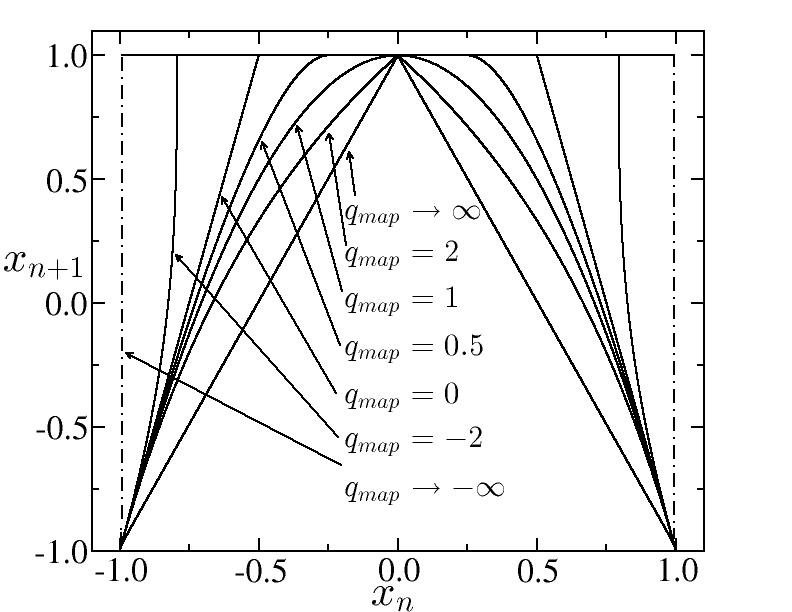
Figure 1: $x_{n+1}$ as a function of $x_{n}$ for the $q$-logistic map (Eq. (4) with $a=2$). The usual parabolic behaviour is recovered at $q_{map}=1$. Tent map is found at $q\to\infty$ (with the peak parameter set to unit). As $q_{map}$ departs from 1 towards $-\infty$ ($q_{map}<1$) the cut-off condition in Eq. (1) yields an increasing region in which $x_{n+1}=1$. For $q_{map}\to-\infty$, $x_{n>0}$ alternates between $1$ and $(1-a)$ $\forall x_{0}\in[-1,1]$. For $q_{map}>1$ the map is discontinuous at $x=0$ and for $q_{map}<1$ the discontinuity is at $|x|=1/2^{1/(1-q)}$.

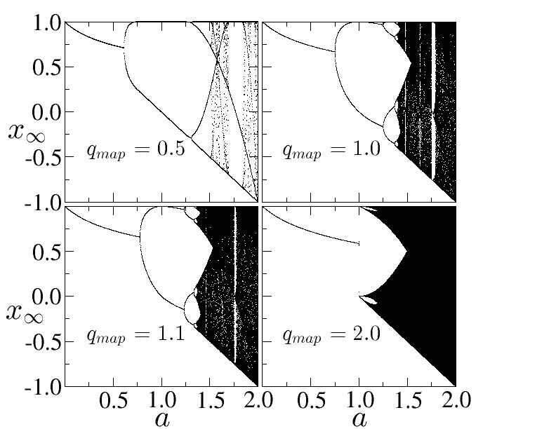
Figure 2: Bifurcation diagrams for different values of $q_{map}$ (indicated). Windows of order inside chaos vanishes as $q_{map}\to 2$. In this paper we explore $q_{map}>1$ but $q_{map}=0.5$ is shown as an instance just to give an idea of the scenario for $q_{map}<1$: the regions of chaos become narrower and the regions of order become dominant.

The $z$-logistic map ($x_{n+1}=1-a|x_{n}|^{z}$, $z>1$, $0<a\leq 2$) [11, 12, 13, 14], is another generalisation of the logistic map for a general power $z>1$ and holds some similarity to the present $q$-logistic map.

Bifurcation diagrams for different values of $q_{map}$ are shown in Fig. 2. As $q_{map}$ goes from 1 (the usual logistic map) to 2, the value of the parameter $a$ for the first bifurcation goes from $a=0.75$ to $a=1$ (it approaches 1 from the left). Also the value of the parameter for the accumulation of bifurcations goes from $a_{c}=1.401155189092\dots$ to $a_{c}=1$ (it approaches 1 from the right). It means that the period doubling cascade becomes narrower until it eventually disappears at $q_{map}=2$. Similar behaviour also happens with the other windows of order inside chaos (where there is tangent bifurcation): they get narrower as $q_{map}$ increases, and eventually disappear for $q_{map}=2$. Complete chaos is preserved at $a=2$, $\forall q_{map}$. The Schwarzian derivative for the $q$-logistic map is given by (see B)

$$(Sf)(x)=\left(q_{map}-\frac{1}{2}q_{map}^{2}\right)\frac{1}{|x|^{2}}\left(1-\frac{4}{4-4|x|^{q_{map}-1}+|x|^{2(q_{map}-1)}}\right).$$ (5)

This expression is negative in the interval $0<q_{map}<2$, and positive for $q_{map}>2$ and for $q_{map}<0$ ($SD(f(x))=0$ for $q_{map}=0$ and for $q_{map}=2$). This means that the route to chaos for $0<q_{map}<2$ is by period doubling bifurcation.

2 Sensitivity to initial conditions

The maximal Lyapunov exponent may be evaluated at the edge of chaos according to (see, for instance, [3])

$$\lambda_{max}=\lim_{N\to\infty}\frac{1}{N}\sum^{N-1}_{i=0}\ln{|f^{\prime}(x_{i})|}$$ (6)

where $f^{\prime}(x)$ is the derivative of the $q$-logistic map,

$$f{{}^{\prime}}(x)=-|x|^{\prime}2a|x|^{-q_{map}}\left[2|x|^{1-q_{map}}-1\right]_{+}^{\frac{q_{map}}{1-q_{map}}}.$$ (7)

$|x|^{\prime}$ is the derivative of the absolute value function: $|x|^{\prime}=1$ for $x>0$ and $|x|^{\prime}=-1$ for $x<0$. For values of the control parameter $a$ different from critical ones, the sensitivity to initial conditions are characterised by exponential divergence at regions of chaos and exponential decay at regions of order, i.e., positive or negative Lyapunov exponent $\lambda_{1}$ (subscript $1$ will be clear in the following) in

$$\xi(t)=\lim_{\Delta x(0)\to 0}\frac{\Delta x(t)}{\Delta x(0)}=e^{\lambda_{1}t}.$$ (8)

At the edge of chaos it was proposed that the divergence follows an asymptotic power-law (in fact a $q$-exponential law) [2] characterising a slow dynamics,

$$\xi(t)=e_{q_{sen}}^{\lambda_{q_{sen}}t}=(1+(1-q_{sen})\lambda_{q_{sen}}t)^{\frac{1}{1-q_{sen}}},$$ (9)

where $\Delta x(0)$ represents the distance between two neighbouring initial conditions and $sen$ stands for sensitivity to initial conditions ($q_{sen}\leq 1$). Eq. (8) is recovered at $q_{sen}=1$ (see A) and this is the reason for the subscript $1$ in $\lambda_{1}$, Eq. (8). As a graphical representation of the sensitivity, it can be defined the variable $L$ as [2]:

$$L=\sum^{N-1}_{i=0}\ln{|f^{\prime}(x_{i})|}.$$ (10)

Figure 3 shows five instances of $L$ vs. $\ln N$. For $q_{map}=2$ (Fig. 3d) the dependence of $L$ on $N$ is very slow and cannot be seen up to $N=2^{15}$ (the upper limit of the figures). For $q_{map}>2$ it is possible to have coexistence of attractors according to the control parameter $a$: depending on the initial conditions, $L$ may be increasingly positive or decreasingly negative. Fig 3f shows that there is a linear dependence of $L$ on $N$ but with different slopes for the cases $L>0$ and $L<0$. For values of $a>1.07499\ldots$, $L<0$ is never exhibited. Coexistence of attractors was also found in [15] for a different deformation of the logistic map (the authors also call their deformation as $q$-logistic map).

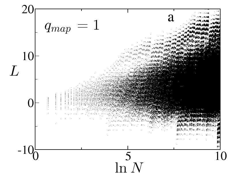
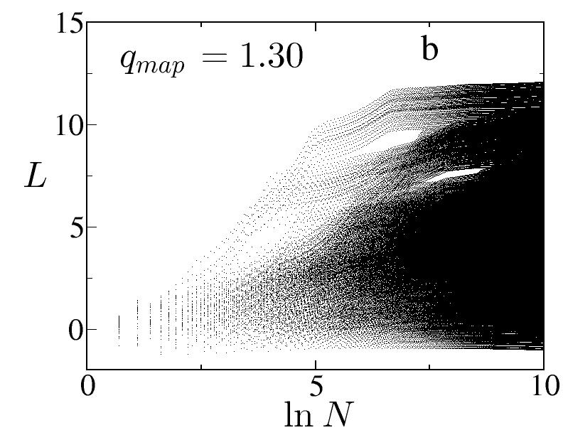
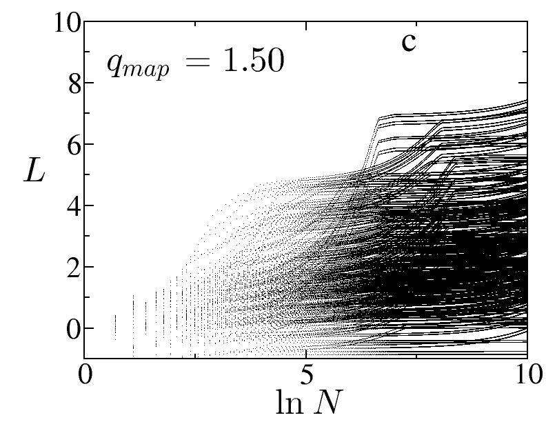
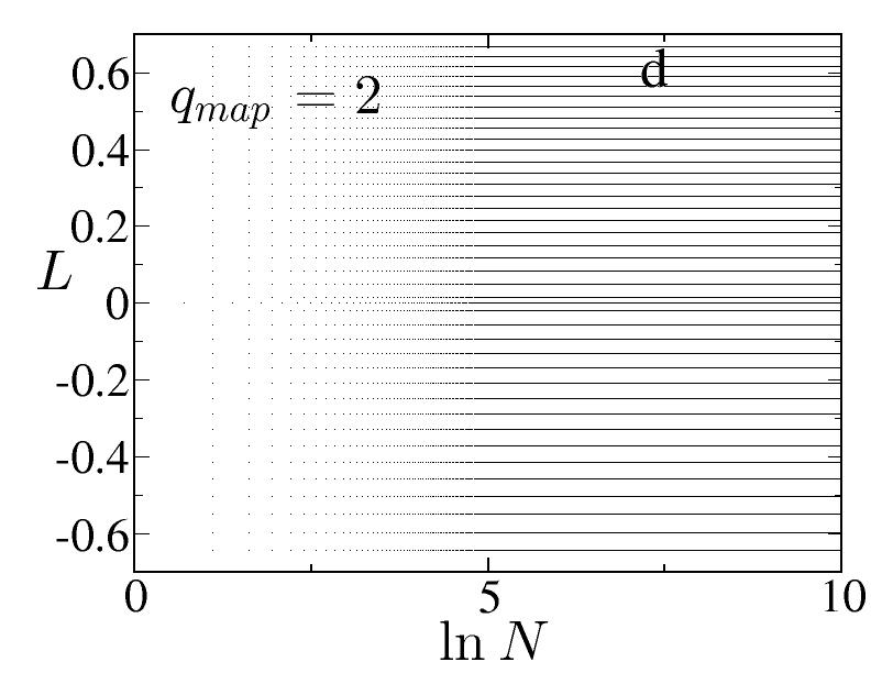
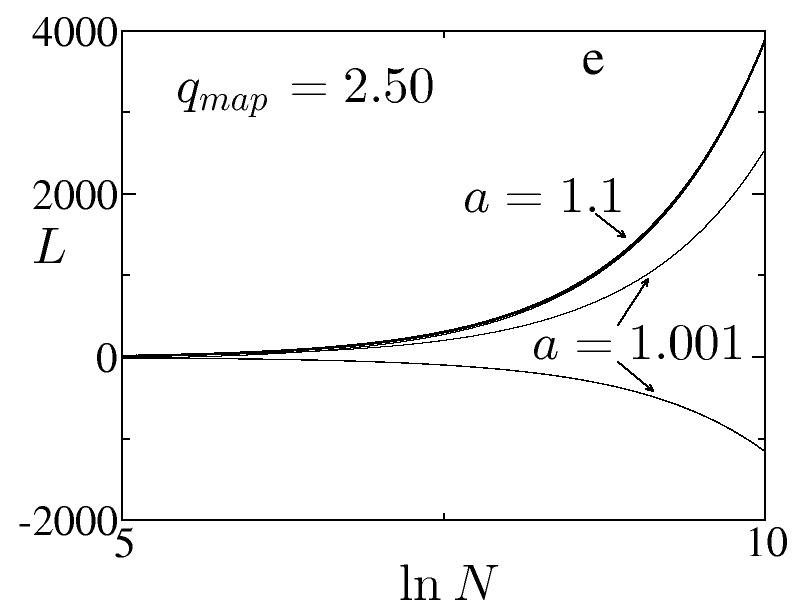
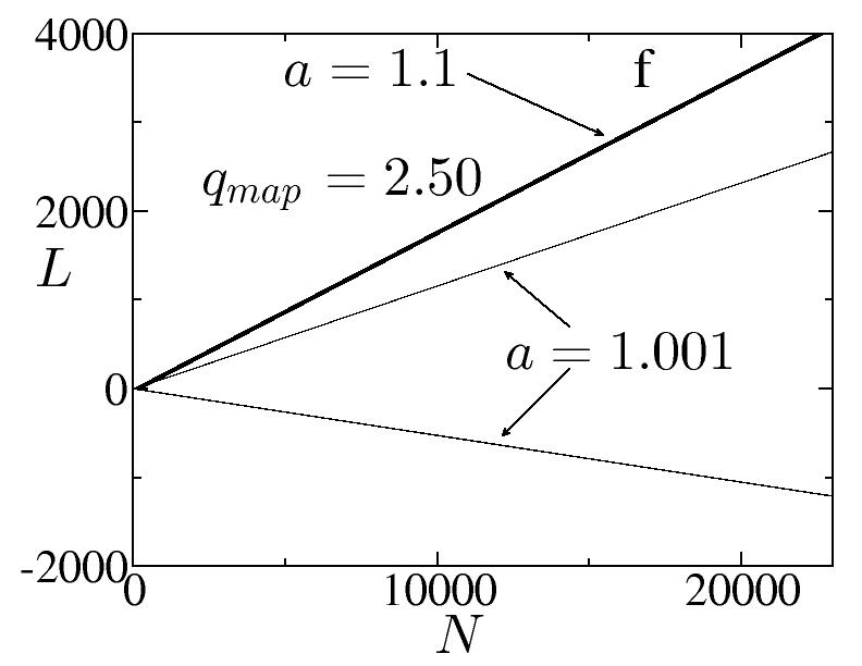
Figure 3: Sensitivity to initial conditions as defined by variable $L$ (Eq. (10)) for different values of $q_{map}$ (indicated). 40 initial conditions are used. For $q_{map}=2.5$ (figures e and f) two values of the control parameter $a$ are presented. It can be seen that it is possible to have coexistence of attractors for a certain ensemble of initial conditions (for $a=1.001$), one with $L>0$ and the other with $L<0$. The same value of $q_{map}=2.5$ and with $a=1.1$, the initial conditions always lead to $L>0$. Fig. f shows linear dependence of $L$ with $N$. Slopes (in absolute values) for $a=1.001$ for $L>0$ and $L<0$ differ.

Lyapunov exponents are displayed in Fig. 4 showing transitions from order to chaos. The figures show that these transitions become sparse as $q_{map}$ departures from unit, and for $q_{map}=2$ there is only one transition (robust chaos)[16]. Fig. 4f shows coexistence of attractors for $q_{map}=2.5$.

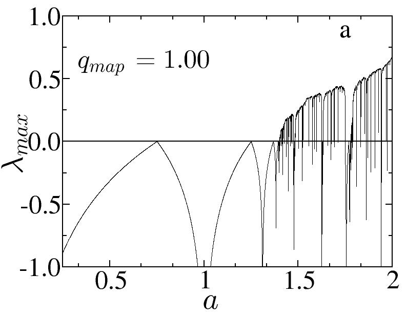
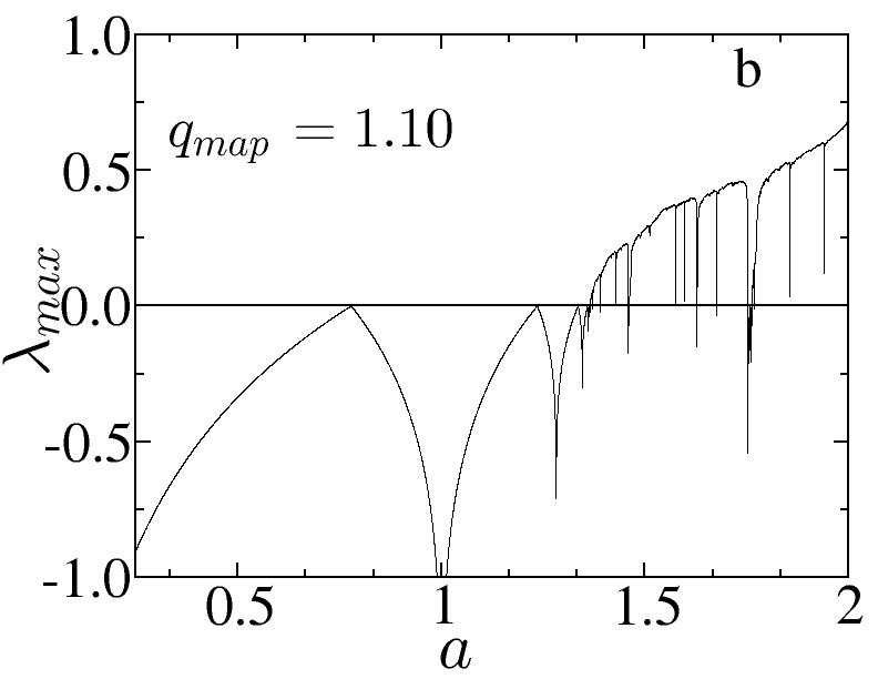
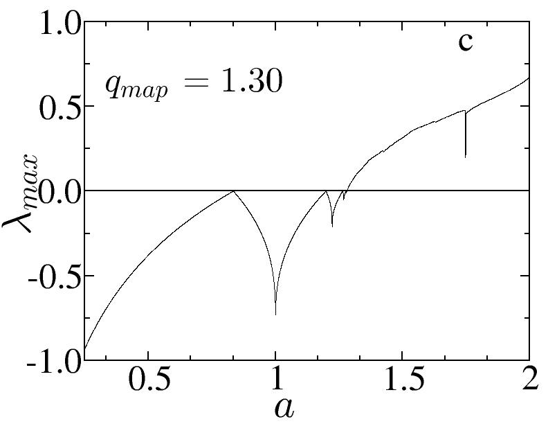
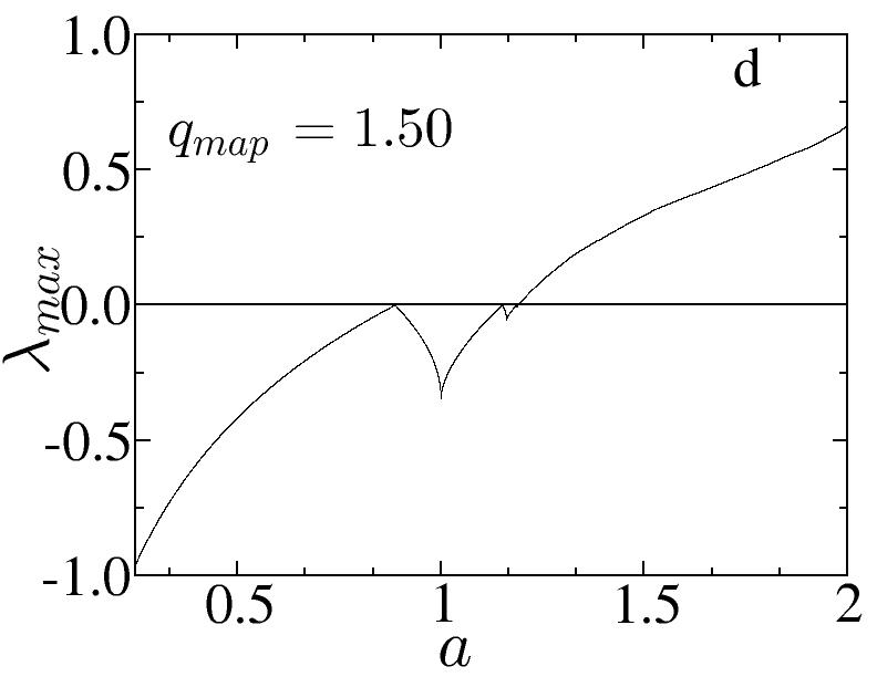
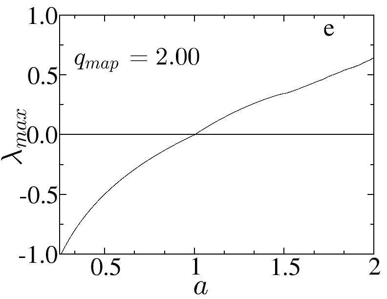
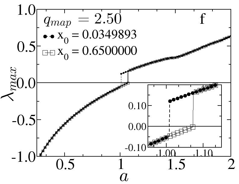
Figure 4: Lyapunov exponent as a function of the control parameter $a$ for different values of $q_{map}$ (indicated). Up to the time limit used in Eq. (6), the almost vertical line in Fig. c at $a=1.7477$ does not crosses zero, but it does present negative values if the calculation is done with a greater precision (it was used $t=2^{18}$ and $\Delta a=2\times 10^{-4}$). Fig. f exhibits coexistence of attractors for two different initial conditions. It’s inset is an amplification of the region of coexistence of attractors for two initial conditions (indicated as full circles and open squares).

Figure 5 illustrates the first point of accumulation of period doubling bifurcation $a_{c}$ as a function of $q_{map}$. For $1<q_{map}<2$, the behaviour is ordinary in the sense that for $a<a_{c}$, $L<0$, and for $a$ slightly greater than $a_{c}$, $L>0$. For $q_{map}>2$ a different behaviour appears: order is found for $a<1$ (region below the solid line), while chaos is found above the dashed line. The region in-between presents coexistence of ordered and chaotic behaviours, depending on the initial conditions (see figures 3e, 3f and 4f).

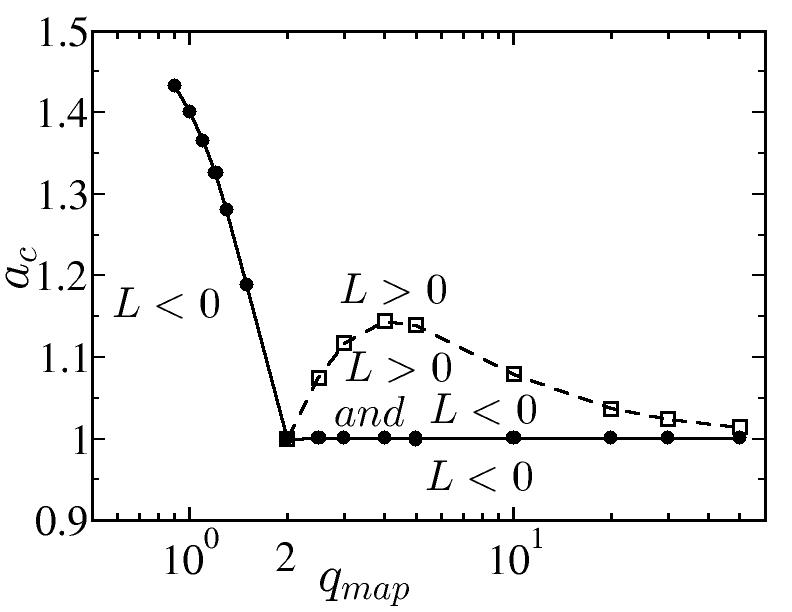
Figure 5: Dependence of the first point of accumulation of period doubling bifurcation $a_{c}$ on $q_{map}$. For $q_{map}>2$ there is a region that exhibits coexistence of attractors depending on the initial conditions. Values of $L$ for this figure were calculated without transient time and final time $t_{end}=2^{18}$, and increments for the control parameter $\Delta{a}=10^{-7}$. Critical point is taken as that for which $0<\lambda_{max}<5\times 10^{-5}$.

Table 1 shows the range of the critical points $a_{c}$ (first point of accumulation of bifurcations) for different values of $q_{map}$. The value of $a_{c}$ is between $a_{-}$ and $a_{+}$. The fourth column shows adopted value for $a_{c}$. For the evaluation of $a_{c}$ listed in Table 1, the Lyapunov exponents were calculated with a transient time of $t_{trans}=2^{23}$ and a final time of $t_{end}=2^{23}$ (the values of the Table are more accurate than those of Fig. 5). Initial condition was fixed in $x_{0}=0.65$ for all cases.

Table 1: Critical points

$q_{map}$	$a_{-}$		$a_{+}$		$a_{c}$
1.00	1.	40115518	1.	40115520	1.	401155189092
1.01	1.	3977569	1.	3977571	1.	397757026
1.02	1.	3943177	1.	3943179	1.	394317802
1.03	1.	3908370	1.	3908372	1.	390837098
1.04	1.	3873144	1.	3873146	1.	387314512
1.05	1.	3837496	1.	3837498	1.	383749669
1.10	1.	3652805	1.	3652807	1.	365280586
1.20	1.	3250906	1.	3250908	1.	325090670
1.30	1.	2811360	1.	2811362	1.	281136143
1.40	1.	2353387	1.	2353389	1.	235338767
1.45	1.	2125150	1.	2125152	1.	21251512
1.50	1.	1900820	1.	1900822	1.	1900822

In Fig. 6 we show the cycle 3 window for $q_{map}=1.25$. This window of order inside chaos (as well as all the others) becomes narrow: in order to identify the Lyapunov exponent in this instance it was necessary to give increments of $\Delta a=1.0\times 10^{-8}$ and $t_{end}=2^{23}$, with a transient $t_{trans}=2^{23}$. Identification of windows of order in this $q$-logistic map is computationally time consuming as $q_{map}$ departs from unit.

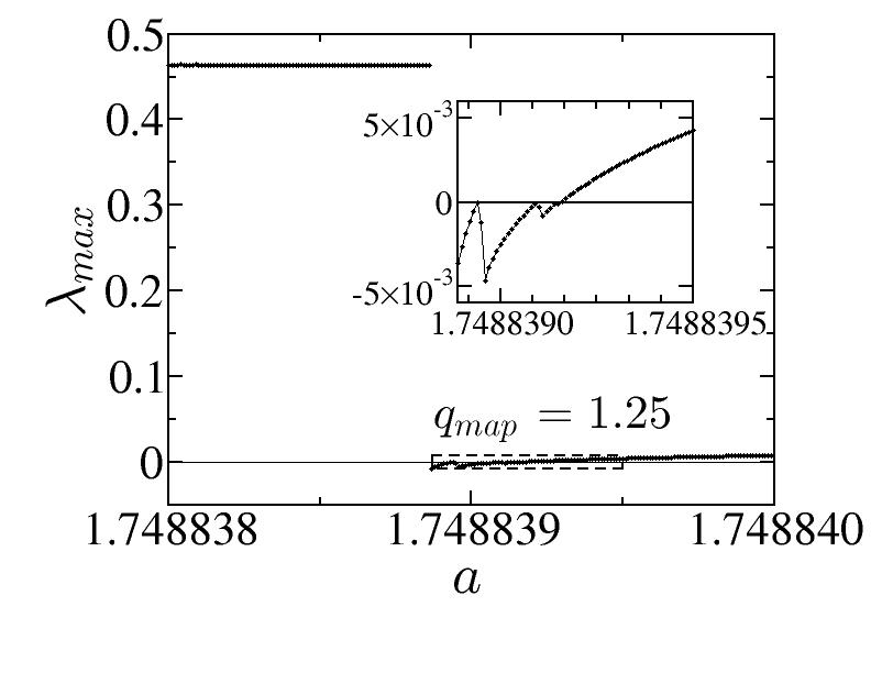
Figure 6: Maximal Lyapunov exponent for $q_{map}=1.25$ at the vicinity of the largest window, of cycle 3, with increments of $\Delta a=1.0\times 10^{-8}$. It was used a transient time of $t_{trans}=2^{23}$ and the time used to estimate the Lyapunov exponent $t_{end}=2^{23}$ (with lower time intervals the transition from negative to positive Lyapunov exponent cannot be seen). Inset corresponds to the dashed rectangle in the main panel and shows points of zero Lyapunov exponents that corresponds to period doubling bifurcation.

3 Entropy production

Parameter $q_{ent}$ (from entropy) in Tsallis entropy [4]

$$S_{q}=k\frac{1-\sum_{i=1}^{W}p_{i}^{q}}{q-1}$$ (11)

($W$ is the number of microstates and $p_{i}$ is the probability of microstate $i$; we use $k=1$ without loss of generality) is estimated according to the method developed in [17]. It consists in calculating the rate of increase of entropy, which must be finite for a large (virtually infinite) system. The phase space ($x_{n}\in[-1,1]$) is divided into $W$ cells, with $N$ points (initial conditions) inside one of them. As time evolves, Tsallis entropy $S_{q}$ is calculated for many values of $q$. Calculation is done again with $N$ points inside another initial cell, and this process is repeated for each cell of a certain ensemble called “best initial condition cells” (the definition of “best initial condition cells” is: the integrated number of occupied cells must be greater than a certain (arbitrary) threshold, the most visited cells). Then it is taken the average of entropy for each time step, and this average is finally plotted against time, for various values of $q$ (see Fig. 7 for an instance). There is only one special value of $q$ for which the increase of $S_{q}$ is linear in the macroscopic limit, that is, the production of entropy $\kappa_{q}=\lim_{t\to\infty}\lim_{W\to\infty}\lim_{N\to\infty}S_{q}/t$ remains finite. This special value is identified with $q_{ent}$ (see [17] for details; in that paper, $q_{ent}$ is called $q^{*}$). For values of the control parameter $a$ that corresponds to chaotic behaviour $q_{ent}=1$, so ordinary Boltzmann-Gibbs-Shannon entropy is the proper one to be used. This is not the case at the edge of chaos ($a=a_{c}$), which we are interested in this work, and the value of $q_{ent}$ which yields linear growth of entropy (and consequently finite rate at the macroscopic limit) is smaller than one (for the ordinary logistic map, $q_{map}=1$, at the edge of chaos, $q_{ent}=0.2445...$). We applied this procedure to the $q$-logistic map. The result of this procedure for various values of $q_{map}$ is presented in Fig. 8.

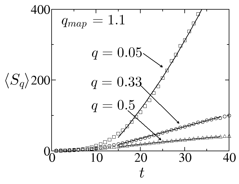
Figure 7: Rate of increase of entropy for $q_{map}=1.1$. We found $q_{ent}=0.33$. This value is found by fitting a parabola $\langle S_{q}(t)\rangle=a+bt+ct^{2}$ for the time interval $15\leq t\leq 38$ (the same used in [17]). Initial times are always left out of calculation because the concavity is always positive at that region. For $q<q_{ent}$ the concavity of the curve is positive (squares, $c>0$) and thus the rate of growth of entropy diverges at the macroscopic limit, which is unphysical. For $q>q_{ent}$, the concavity is negative (triangles, $c<0$), thus the rate of growth of entropy is zero at the macroscopic limit, which is also unphysical. $c=0$ is shown as circles.

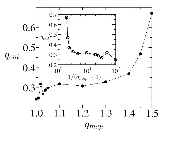
Figure 8: $q_{ent}$ as a function of $q_{map}$. Inset shows abscissa in a different scale (note that abscissa is in log scale). The value at $q_{map}=1.02$ may have numerical imprecision. Lines are only guide to the eyes.

The integrated number of occupied cells, used to identify the best initial condition cells, is shown in Fig. 10. We see a reduction of the number of visited cells as $q_{map}$ goes from one to two and a change in the displayed pattern. Fig. 10 shows number of cells with visits greater than 5000 as a function of $q_{map}$.

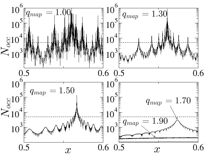
Figure 9: Integrated number of visits per cell for five cases ($q_{map}=1,1.30,1.50,1.70,1.90$). Phase space is divided into $W=10^{5}$ cells, each one contains $10^{6}$ points uniformly distributed. Time evolves up to 50 iterations. Figures show $x\in[0.5,0.6]$ just for better visualisation.

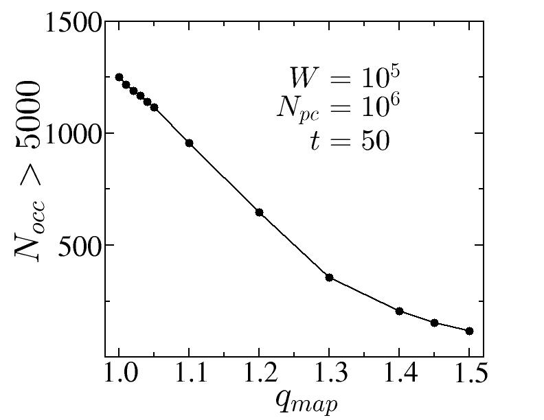
Figure 10: Number of cells with more than 5000 visits in a run of 50 iterations as a function of $q_{map}$. $N_{pc}=10W$ is the number of initial conditions per cell. Dashed horizontal line in Fig. 10 indicates the threshold of 5000 visits per cell.

4 Relaxation to the critical attractor

Relaxation to the critical attractor was presented at [6] and basically consists in the division of the phase space [-1,1] into $W$ cells and take an ensemble of $N$ initial conditions uniformly distributed in the entire phase space (thus maximal entropy). Time evolution leads to the decreasing of the number of occupied cells $W_{occ}(t)$ according to a power-law with log-periodic oscillations ($W_{occ}(0)=W$). It is supposed [6] that the power-law is the asymptotic limit of a $q$-exponential, and the parameter is denoted as $q_{rel}$, for relaxation ($q_{rel}>1$):

$$W_{occ}(t)=(1+(1-q_{rel})K_{q_{rel}}t)^{\frac{1}{1-q_{rel}}},$$ (12)

$K_{q_{rel}}$ is the inverse of a characteristic time. Figure 11 presents the results for the fraction of occupied cells $W_{occ}(t)/W_{occ}(0)$ for different values of $q_{map}$ at their corresponding critical points. Log-periodic oscillations present increasing periods for $q_{map}\to 2$. The slope in the log-log plot (Fig. 11a) at the region of the log-periodic oscillations is used to estimate $q_{rel}$ as $\mbox{slope}=1/(1-q_{rel})$. Fig. 11b presents $q_{rel}$ as a function of $q_{map}$.

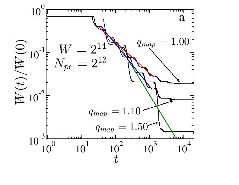
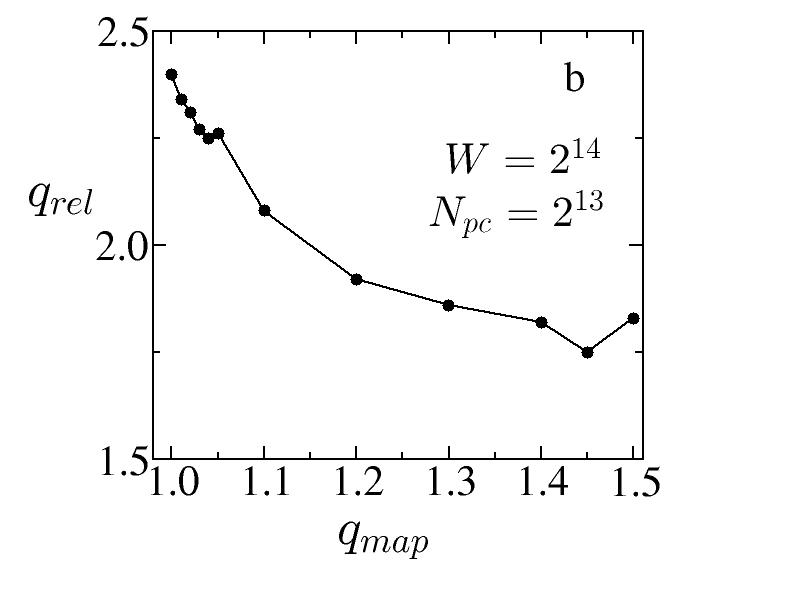
Figure 11: Relaxation to the critical attractor at the edge of chaos. Fig. a is a log-log plot of $W_{occ}(t)/W_{occ}(0)\times t$ for three different values of $q_{map}$. It can be seen the results of regression of power-laws, whose slopes are identified as $1/(1-q_{rel})$. Fig. b shows $q_{rel}$ as a function of $q_{map}$. It was used $W=2^{14}$ and number of initial conditions per cell $N_{pc}=2^{13}$. Lines are only guide to the eyes. Fluctuations in the curve of Fig. b are due to inaccuracy — the results are very sensitive to small changes in the characteristic parameters.

The procedure for estimating $q_{rel}$, that is, the shrinking of the number of occupied cells, is also used to estimate the fractal dimension $d_{f}$ at the edge of chaos (it is a kind of box counting method). $W_{occ}(\infty)$ increases with $W_{occ}(0)$ according to $W_{occ}(\infty)\propto[W_{occ}(0)]^{d_{f}}$. Fractal dimension decreases with $q_{map}$ as shown in Fig. 12.

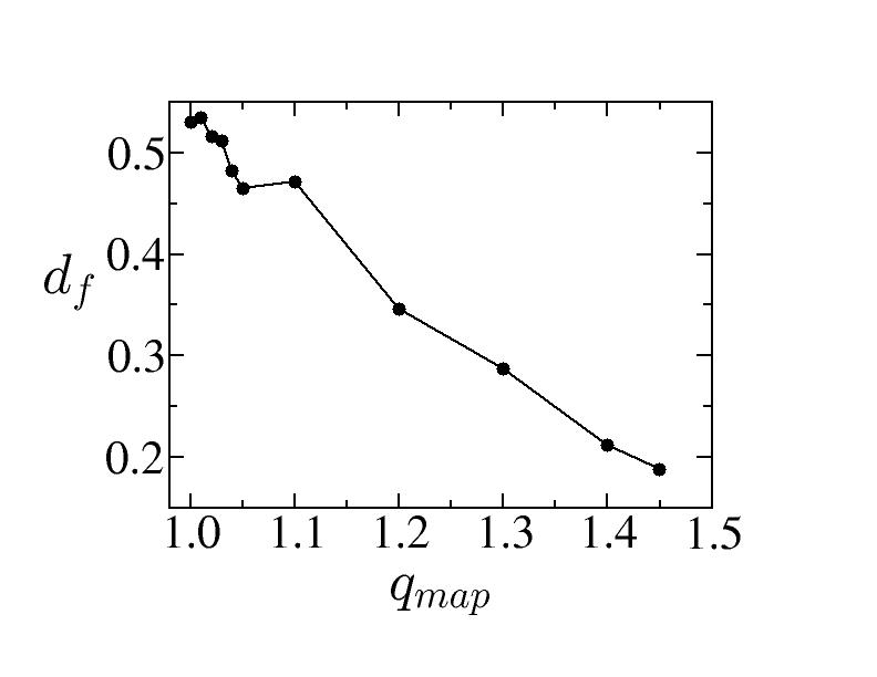
Figure 12: Fractal dimension at the edge of chaos as a function of $q_{map}$. For the usual logistic map ($q_{map}=1$), $d_{f}(a_{c})=0.53665$. Lines are only guide to the eyes. Fluctuations in the curve are due to inaccuracy — the method is very sensitive to small changes in the characteristic parameters.

5 Final remarks

The generalisation of the logistic map by means of the $q$-product introduces some interesting features in its dynamical behaviour. Our analysis is focused on $q_{map}>1$. In this region, the windows of order inside chaos become narrower as $q_{map}$ increases until all of them disappear and the map becomes the tent map. For $q_{map}<1$ (not analysed in this paper) the opposite behaviour occurs: the regions of chaos become narrower and order dominates the scenario. A remarkable feature of the $q$-logistic map is to continuously pass from a map with a variety of behaviours, such as period doubling bifurcation, multifractality and power-law like sensibility to initial conditions at the edge of chaos (the logistic map), to a robust map (the tent map). We have calculated the sensitivity to initial conditions, the rate of entropy growth, the relaxation to the critical attractor and the fractal dimension at the edge of chaos. These methods permit to estimate the parameters $q_{ent}$ and $q_{rel}$ for different values of $q_{map}$. The entropy parameter and the relaxation parameter are two indices that appear within the context of nonextensive statistical mechanics and the understanding of their dependence on the control parameters of the system may lead to their a priori determination. Some other evaluations for this $q$-logistic map remains to be done, e.g. the dependence of $q_{rel}$ on the coarse graining $W$ and its relation to $q_{sen}$ (as in [12] for the $z$-logistic map, and as in [18, 19] for the Hénon map), the probability distributions of sums of iterates as in [20, 21], multifractality as it was done in [22], and tangent bifurcations.

Appendix A Special limits for the $q$-product

The limit $q\to v$ where $v$ is one of the following $\{-\infty,1,\infty\}$ for the $q$-product $x\otimes_{q}x$ as it appears in the $q$-logistic map, Eq. (4) and also in Eq. (1) with $y=x$, leads to $\{0^{0},{1}^{\infty},{\infty}^{0}\}$ respectively. The indeterminates can easily be solved by means of a simple trick that is to rewrite the $q$-product as

$$x\otimes_{q}x=[2|x|^{1-q}-1]_{+}^{\frac{1}{1-q}}=h(q)^{g(q)}$$ (13)

with $h(q)=[2|x|^{1-q}-1]_{+}$ (note that $h(q)\geq 0$ due to the cut-off condition in Eq. (1)) and $g(q)=\frac{1}{1-q}$. Of course $h$ is a function of $q$ and $x$ but for now we are not interested in the dependency on $x$, so we omit it. We also omit the subscript of $q$ for the sake of brevity. Then

$$\lim_{q\to v}[2|x|^{1-q}-1]_{+}^{\frac{1}{1-q}}=e^{\lim_{q\to v}g(q)\ln h(q)}.$$ (14)

Straightforward application of L’Hospital rule leads to (we remind the reader that $|x|\leq 1$)

$$\lim_{q\to v}x\otimes_{q}x=\left\{\begin{array}[]{ll}\left.\begin{array}[]{cl}1,&\mbox{if }|x|=1\\ 0,&\mbox{if }|x|<1\end{array}\right\}&\mbox{for }v=-\infty,\\ \begin{array}[]{ll}x^{2},&\end{array}&\mbox{for }v=1,\\ \begin{array}[]{ll}|x|,&\end{array}&\mbox{for }v=\infty.\end{array}\right.$$ (22)

L’Hospital rule must be applied twice in the case $v=\infty$. A similar procedure applied to Eq. (9), now with $h(q)=1+(1-q_{sen})\lambda_{q_{sen}}t$ and $g(q)=\frac{1}{1-q_{sen}}$, leads to Eq. (8).

Appendix B Schwarzian derivative for the $q$-logistic map

The Schwarzian derivative is defined by

$$(Sf)(x)=\frac{f^{{}^{\prime\prime\prime}}}{f^{{}^{\prime}}}-\frac{3}{2}\left(\frac{f^{{}^{\prime\prime}}}{f^{{}^{\prime}}}\right)^{2}.$$ (23)

The function $f(x)=1-a\left(x\otimes_{q_{map}}x\right)$ represents the $q$-logistic map and it may be written as $f(x)=1-ah(x)^{g(q)}$ with $h(x)$ and $g(q)$ given by Eq. (13) — now we are interested in the dependency of $h$ on $x$. The three first derivatives of $f(x)$ are given by

$$\begin{array}[]{lcl}f^{{}^{\prime}}(x)&=&-a\frac{1}{1-q}h^{\frac{q}{1-q}}h^{{}^{\prime}}\\ &&\\ f^{{}^{\prime\prime}}(x)&=&-a\frac{1}{1-q}\left(\frac{q}{1-q}h^{\frac{2q-1}{1-q}}\left(h^{{}^{\prime}}\right)^{2}+h^{\frac{q}{1-q}}h^{{}^{\prime\prime}}\right)\\ &&\\ f^{{}^{\prime\prime\prime}}(x)&=&-a\frac{1}{1-q}\frac{q(2q-1)}{(1-q)^{2}}h^{\frac{3q-2}{1-q}}\left(h^{{}^{\prime}}\right)^{3}\\ &&-a\frac{1}{1-q}3\frac{q}{1-q}h^{\frac{2q-1}{1-q}}h^{{}^{\prime}}h^{{}^{\prime\prime}}\\ &&-a\frac{1}{1-q}h^{\frac{q}{1-q}}h^{{}^{\prime\prime\prime}}\end{array}$$ (31)

with $h^{{}^{\prime}}=|x|^{\prime}2(1-q)|x|^{-q}$, $h^{{}^{\prime\prime}}=-2q(1-q)|x|^{-1-q}$ and $h^{{}^{\prime\prime\prime}}=|x|^{\prime}2q(1-q)(1+q)|x|^{-2-q}$. Substitution in Eq. (23) leads to

$$(Sf)(x) = \frac{4q(2q-1)}{|x|^{2q}[2|x|^{1-q}-1]_{+}^{2}}-\frac{6q^{2}}{|x|^{1+q}[2|x|^{1-q}-1]_{+}}+\frac{q(1+q)}{|x|^{2}}$$ (32)

$$-\frac{3}{2}\left(\frac{2q}{|x|^{q}[2|x|^{1-q}-1]_{+}}-\frac{q}{|x|}\right)^{2}$$

This expression may be rearranged as in Eq. (5) that is more convenient to analyse its signal. The Schwarzian derivative for the $q$-logistic map presents a divergence at $x=0$ for $1\leq q<2$ and a divergence at $x=0$ and at $x=\pm 1/2^{1/(1-q)}$ for $q<1$. The case $q_{map}=1$ corresponds to the Schwarzian derivative for the usual logistic map, $(Sf)(x)=-3/(2x^{2})$, as can be easily verified.

References

References

- [1] Hilborn R 2000 Chaos and Nonlinear Dynamics: An Introduction for Scientists and Engineers (Oxford University Press, USA)
- [2] Tsallis C, Plastino A R and Zheng W M 1997 Chaos Sol. Fract. 8 885–891
- [3] Beck C and Schlögl F 1995 Thermodynamics of Chaotic Systems: An Introduction (Cambridge Nonlinear Science Series) (Cambridge University Press)
- [4] Tsallis C 1988 J. Stat. Phys. 52 479–487
- [5] Tsallis C 2009 Introduction to Nonextensive Statistical Mechanics: Approaching a Complex World 1st ed (Springer)
- [6] de Moura F, Tirnakli U and Lyra M L 2000 Phys. Rev. E 62 6361–6365
- [7] Nivanen L, Le Méhauté A and Wang Q A 2003 Rep. Math. Phys. 52 437–444
- [8] Borges E P 2004 Physica A 340 95–101
- [9] Suyari H and Tsukada M 2005 Information Theory, IEEE Transactions on 51 753–757
- [10] Umarov S, Tsallis C and Steinberg S 2008 Milan Journal of Mathematics 76 307–328
- [11] Costa U M S, Lyra M L, Plastino A R and Tsallis C 1997 Phys. Rev. E 56 245–250
- [12] Borges E P, Tsallis C, Añaños G F J and de Oliveira P M C 2002 Phys. Rev. Lett. 89 254103
- [13] da Silva C R, da Cruz H R and Lyra M L 1999 Braz. J. Phys. 29 144–152
- [14] Tirnakli U and Tsallis C 2006 Phys. Rev. E 73 037201
- [15] Jaganathan R and Sinha S 2005 Phys. Lett. A 338 277–287
- [16] Banerjee S, Yorke J and Grebogi C 1998 Phys. Rev. Lett. 80 3049–3052
- [17] Latora V, Baranger M, Rapisarda A and Tsallis C 2000 Phys. Lett. A 273 97–103
- [18] Borges E P and Tirnakli U 2004 Physica D 193 148–152
- [19] Borges E P and Tirnakli U 2004 Physica A 340 227–233
- [20] Tirnakli U, Beck C and Tsallis C 2007 Phys. Rev. E 75 040106
- [21] Tirnakli U, Tsallis C and Beck C 2009 Phys. Rev. E 79 056209
- [22] Lyra M and Tsallis C 1998 Phys. Rev. Lett. 80 53–56