Analytical approach for treating unitary quantum systems with initial mixed states

Abstract

The mixed states are important in quantum optics since they frequently appear in the decoherence problems. When one of the components of the system is prepared in the mixed state and the evolution operator of this system is not available, one cannot deduce the density matrix. We present analytical approach to accurately solve this problem. The approach can be applied on the condition that the Schrödinger’s equation of the system is solvable with any arbitrary initial state. In deriving the solution we exploit the fact that any mixed state can be expressed in terms of a phase state. The approach is illustrated by deriving the density matrix of a single-mode heat environment interacting asymmetrically with two qubits. Our results are in good agreement with the available results in the literature. This approach opens new perspectives for treating complicated systems and may impact other applications in the quantum theory.

Key words: mixed state, thermal state, density matrix, Schrodinger equation, entanglement, two-qubit

I Introduction

In quantum theory, the state of the system has two categories; namely pure state and mixed state. A pure state implies perfect knowledge of the system. For the mixed case, we do not have enough information to specify the state of the system completely and hence cannot form its wavefunction. In this situation, we can only describe the system via the density matrix $\hat{\rho}_{f}$. Mixed state frequently appears in the decoherence problems, e.g., bernet . We can obtain the mixed state, which is associated with any state, by considering its phase to be totally randomized. The best example of the mixed state is the thermal field, which represents an electromagnetic radiation emitted by a source at temperature $T$. The examination of a quantum beam with a thermal noise is an important topic from both theoretical and practical points of view, e.g. thermal .

In the quantum information theory, a considerable attention has been paid to the entanglement of the bipartite and the multipartite systems in which one of the subsystems exists initially in the thermal equilibrium amesen ; lee1 ; lee2 . The conclusion of all these studies is that it is possible for the thermal field, which is a highly chaotic field, to induce entanglement between qubits. The previous studies have been limited to the systems whose exact form of the evolution operators is obtainable amesen ; lee2 . For the other systems the solution is difficult or even impossible. For some few systems of the latter, one has to use the numerical methods to solve the master equation of the system lee1 , but the results cannot be totally trusted. In this paper we develop, for the first time, a simple analytical approach solving this problem exactly. This approach can provide the dynamical density matrix of the unitary quantum system whose one of its components is initially in the mixed state such as the thermal field. It works only when the Schrödinger’s equation of the system for any arbitrary initial state is solvable. Furthermore, the approach can be applied as an alternative technique for finding the solution of the systems whose evolution operators exist but they are very complicated. For instance, the evolution of the mixed field with the multi-level atoms, e.g. three-level atom and four-level atom, etc.

In section II we describe the approach in details. In section III we give an application for the approach by solving specific problem. The example, which we have considered, is that the problem of the two atoms in the cavity interact asymmetrically with the thermal field. The reason behind this choice is that this system is a subject of the current research in relation to entanglement amesen ; lee1 ; lee2 . Thus, we can easily validate the approach by comparing our results with the available results in the literature.

II Description of the approach

In this section, we describe how one can deduce the density matrix of the unitary quantum system whose one of its components is initially prepared in the thermal state. Before going into details, let us briefly state some properties of the thermal field. The thermal field has a diagonal expansion in terms of Fock states as bernet :

$$\hat{\rho}_{f}=\sum\limits_{n=0}^{\infty}p(n)|n\rangle\langle n|=\frac{1}{\pi}\int\limits_{0}^{\pi}|z(\phi)\rangle\langle z(\phi)|d\phi,$$ (1)

where $p(n)$ is the photon-number distribution of the thermal field and $|z(\phi)\rangle$ is the associated phase state having the form:

$$|z(\phi)\rangle=\sum\limits_{n=0}^{\infty}\sqrt{p(n)}\exp(in\phi)|n\rangle=\sum\limits_{n=0}^{\infty}C_{n}(\phi)|n\rangle,$$ (2)

where

$$C_{n}(\phi)=\sqrt{p(n)}\exp(in\phi),\quad p(n)=\frac{\bar{n}^{n}}{(1+\bar{n})^{n+1}}$$ (3)

and $\bar{n}$ is the mean-photon number of the thermal field having the form $\bar{n}=(e^{\hbar w/k_{b}T}-1)^{-1}$ and $k_{b}$ is the Boltzmann’s constant. It is obvious that $\bar{n}$ increases by increasing the temperature $T$.

Now we are in a position to explain the approach. Assume that we have a bipartite system whose Hamiltonian is $\hat{H}_{db}$, where $d$ and $b$ stand for the field and the other party, respectively. These two components are initially prepared in the states $|\psi_{d}(0)\rangle$ and $|\psi_{b}(0)\rangle$. The Schrödinger’s equation of this system is solvable and hence we can obtain the wavefunction as $|\psi(t)\rangle$. From the basic concepts of the quantum mechanics we have:

$$|\psi(t,0)\rangle=\hat{U}(t,0)|\psi_{d}(0)\rangle\bigotimes|\psi_{b}(0)\rangle,$$ (4)

where $\hat{U}(t,0)$ is the evolution operator of the system regardless if we can deduce its explicit form or not. Under these assumptions we can solve this system accurately if the party $d$ is initially prepared in the thermal field $\hat{\rho}_{f}$ instead of $|\psi_{d}(0)\rangle$. In this case the initial state of the system reads:

$$\hat{\rho}(0)=\hat{\rho}_{f}\bigotimes|\psi_{b}(0)\rangle\langle\psi_{b}(0)|=\frac{1}{\pi}\int\limits_{0}^{\pi}|z(\phi)\rangle\langle z(\phi)|\bigotimes|\psi_{b}(0)\rangle\langle\psi_{b}(0)|d\phi.$$ (5)

Under the evolution operator $\hat{U}(t,0)$, the system in the initial state (5) evolves as:

$$\hat{\rho}(t)=\hat{U}(t,0)\hat{\rho}(0)\hat{U}^{\dagger}(t,0)=\frac{1}{\pi}\int\limits_{0}^{\pi}|\psi_{z}(t,\phi)\rangle\langle\psi_{z}(t,\phi)|d\phi,$$ (6)

where $|\psi_{z}(t,\phi)\rangle=\hat{U}(t,0)|z(\phi)\rangle\bigotimes|\psi_{b}(0)\rangle$. Our target is to deduce the wavefunction $|\psi_{z}(t,\phi)\rangle$. If the explicit form of $\hat{U}(t,0)$ is available, the solution is straightforward. If it is not, we can solve the Schrödinger’s equation for the initial condition $|z(\phi)\rangle$ and $|\psi_{b}(0)\rangle$. We have to emphasize if the system is solvable for the arbitrary state $|\psi_{d}(0)\rangle$, it will be automatically solvable for the state $|z(\phi)\rangle$. This is based on the fact that any state of the field is just a linear combination of the Fock states weighted by a specific distribution. As soon as we derive $|\psi_{z}(t,\phi)\rangle$ we substitute it into (6) and carry out the integration over the phase $\phi$ to obtain the requested density matrix. From the above description, the theme of the approach we transform the problem of obtaining the dynamical density matrix to that of finding the wavefunction of the system when the field is initially prepared in the state $|z(\phi)\rangle$.

In spite of the simplicity of the approach, it is efficient and able to provide the exact solutions for some non-analytically solvable problems so far. In the following section we show this fact by developing the analytical solution for one of those problems, which has been already numerically treated.

III Example: two-qubit problem

In this section, we apply the approach described in the preceding section to obtain the density matrix of the two-qubit problem. Precisely, we deduce the dynamical density matrix of the system of the single-mode thermal field interacting simultaneously with the two two-level atoms in the cavity in the non-identical fashion. The numerical technique has been exploited for solving this system lee1 , however, here we present the analytical solution. It is worthwhile mentioning that the two-identical-atom version of this system has been already demonstrated, e.g., lee1 ; lee2 ; nf . For the latter the dynamical density matrix of the system has been derived by the Kraus representation kraus . That cannot be applied to the non-identical-atom system. Also, we verify the validity of the approach by comparing some of our results to those in the literature in relation to entanglement. We proceed, under the rotating wave approximation the Hamiltonian describing the system takes the form lee1 ; lee2 ; nf :

$$\begin{array}[]{lr}\frac{\hat{H}}{\hbar}=\hat{H}_{0}+\hat{H}_{I},\\ \\ \hat{H}_{0}=\omega\hat{a}^{\dagger}\hat{a}+\frac{\omega_{a}}{2}(\hat{\sigma}_{1}^{z}+\hat{\sigma}_{2}^{z}),\quad\hat{H}_{I}=\sum\limits_{j=1}^{2}\lambda_{j}(\hat{a}\hat{\sigma}_{j}^{+}+\hat{a}^{\dagger}\hat{\sigma}_{j}^{-}),\end{array}$$ (10)

where $\hat{H}_{0}$ and $\hat{H}_{I}$ are the free and interaction parts of the Hamiltonian, $\hat{\sigma}_{j}^{\pm}$ and $\hat{\sigma}_{j}^{z}$ are the Pauli spin operators of the $j$th atom; $\hat{a}\quad(\hat{a}^{\dagger})$ is the annihilation (creation) operator denoting the cavity mode, $\omega$ and $\omega_{a}$ are the frequencies of the cavity mode and the atomic systems (we consider that the two atoms have the same frequency) and $\lambda_{j}$ is the coupling constant between the $j$th atom and the field. Based on the relation between $\lambda_{1}$ and $\lambda_{2}$ we have two cases; namely asymmetric case ($\lambda_{1}\neq\lambda_{2}$) and symmetric case ($\lambda_{1}=\lambda_{2}$). We should stress that the asymmetric case is closer to experiment than the symmetric one duan . Finally, throughout the investigation we assume that $\omega_{a}=\omega$.

Now, our aim is to deduce the explicit form of the density matrix $\hat{\rho}(t)$ of the Hamiltonian (10) when the field is initially prepared in the thermal field (1) and the atoms are initially in the following mixed state:

$$\hat{\rho}_{a}=\sin^{2}\theta\cos^{2}\vartheta|e_{1},e_{2}\rangle\langle e_{2},e_{1}|+\sin^{2}\theta\sin^{2}\vartheta|g_{1},g_{2}\rangle\langle g_{2},g_{1}|+\cos^{2}\theta|e_{1},g_{2}\rangle\langle g_{2},e_{1}|,$$ (11)

where $|e_{j}\rangle$ and $|g_{j}\rangle$ stand for the excited and the ground atomic states of the $j$th atom, respectively. The variables $\theta$ and $\vartheta$ are phases, which can be specified to give different types of the initial atomic states. The subscript $a$ denotes the atomic system. We should stress that the suggested approach is applicable for any initial atomic state not only (11). Noteworthily, for $\lambda_{1}\neq\lambda_{2}$ we cannot derive the explicit form of the evolution operator of the system $\hat{U}(t,0)$, however, we can solve the Schrödinger’s equation faisala . The latter is the main demand to apply the approach. The whole initial state of the system can be easily written in the form (5). Under the evolution operator $\hat{U}(t,0)$, this initial state evolves as:

$$\begin{array}[]{lr}\hat{\rho}(t)=\hat{U}(t,0)\hat{\rho}(0)\hat{U}^{\dagger}(t,0)\\ \\ =\frac{\sin^{2}\theta\cos^{2}\vartheta}{\pi}\int\limits_{0}^{\pi}|\Psi_{1}(t,\phi)\rangle\langle\Psi_{1}(t,\phi)|d\phi+\frac{\sin^{2}\theta\sin^{2}\vartheta}{\pi}\int\limits_{0}^{\pi}|\Psi_{2}(t,\phi)\rangle\langle\Psi_{2}(t,\phi)|d\phi\\ \\ +\frac{\cos^{2}\theta}{\pi}\int\limits_{0}^{\pi}|\Psi_{3}(t,\phi)\rangle\langle\Psi_{3}(t,\phi)|d\phi,\end{array}$$ (17)

where

$$\begin{array}[]{lr}|\Psi_{j}(t,\phi)\rangle=\hat{U}(t,0)|\Psi_{j}(0,\phi)\rangle,\quad j=1,2,3,\\ \\ |\Psi_{1}(0,\phi)\rangle=|e_{1},e_{2},z(\phi)\rangle,\quad|\Psi_{2}(0,\phi)\rangle=|g_{1},g_{2},z(\phi)\rangle,\quad|\Psi_{3}(0,\phi)\rangle=|e_{1},g_{2},z(\phi)\rangle.\end{array}$$ (21)

Our main concern is to derive the wave functions $|\Psi_{j}(t,\phi)\rangle$. These can be easily obtained by solving the Schrödinger’s equation three times for the given initial conditions as faisala :

$$\begin{array}[]{lr}\mid\Psi_{j}(t,\phi)\rangle=\sum\limits_{n=0}^{\infty}C_{n}(\phi)\left[X_{1}^{(j)}(t,n)\mid e_{1},e_{2},n\rangle+X_{2}^{(j)}(t,n)\mid e_{1},g_{2},n+1\rangle\right.\\ \\ +\left.X_{3}^{(j)}(t,n)\mid g_{1},e_{2},n+1\rangle+X_{4}^{(j)}(t,n)\mid g_{1},g_{2,}n+2\rangle\right],\quad j=1,2,3\end{array}$$ (25)

where

$$\begin{array}[]{lr}X_{1}^{(1)}(t,n)=\mu^{-}_{n}\frac{\cos(t\Omega^{+}_{n})}{2\Lambda_{n}}+\mu^{+}_{n}\frac{\cos(t\Omega^{-}_{n})}{2\Lambda_{n}},\\ X_{2}^{(1)}(t,n)=\frac{-i\lambda_{2}\sqrt{n+1}}{2\Lambda_{n}}\{[4\lambda_{1}^{2}(n+2)-\mu^{-}_{n}]\frac{\sin(t\Omega^{+}_{n})}{\Omega^{+}_{n}}-[4\lambda_{1}^{2}(n+2)-\mu^{+}_{n}]\frac{\sin(t\Omega^{-}_{n})}{\Omega^{-}_{n}}\},\\ X_{3}^{(1)}(t,n)=\frac{-i\lambda_{1}\sqrt{n+1}}{2\Lambda_{n}}\{[4\lambda_{2}^{2}(n+2)-\mu^{-}_{n}]\frac{\sin(t\Omega^{+}_{n})}{\Omega^{+}_{n}}-[4\lambda_{2}^{2}(n+2)-\mu^{+}_{n}]\frac{\sin(t\Omega^{-}_{n})}{\Omega^{-}_{n}}\},\\ X_{4}^{(1)}(t,n)=\frac{2\lambda_{1}\lambda_{2}\sqrt{(n+2)(n+1)}}{\Lambda_{n}}[\cos(t\Omega^{+}_{n})-\cos(t\Omega^{-}_{n})],\\ X_{1}^{(2)}(t,n)=\frac{2\lambda_{1}\lambda_{2}\sqrt{n(n-1)}}{\Lambda_{n-2}}\left[\cos(t\Omega^{+}_{n-2})-\cos(t\Omega^{-}_{n-2})\right],\\ X_{2}^{(2)}(t,n)=\frac{-i\lambda_{1}\sqrt{n}}{2\Lambda_{n-2}}\left\{[4\lambda_{2}^{2}(n-1)+\mu^{+}_{n-2}]\frac{\sin(t\Omega^{+}_{n-2})}{\Omega^{+}_{n-2}}-[4\lambda_{2}^{2}(n-1)+\mu^{-}_{n-2}]\frac{\sin(t\Omega^{-}_{n-2})}{\Omega^{-}_{n-2}}\right\},\\ X_{3}^{(2)}(t,n)=\frac{-i\lambda_{2}\sqrt{n}}{2\Lambda_{n-2}}\left\{[4\lambda_{1}^{2}(n-1)+\mu^{+}_{n-2}]\frac{\sin(t\Omega^{+}_{n-2})}{\Omega^{+}_{n-2}}-[4\lambda_{1}^{2}(n-1)+\mu^{-}_{n-2}]\frac{\sin(t\Omega^{-}_{n-2})}{\Omega^{-}_{n-2}}\right\},\\ X_{4}^{(2)}(t,n)=\frac{\mu^{+}_{n-2}}{2\Lambda_{n-2}}\cos(t\Omega^{+}_{n-2})-\frac{\mu^{-}_{n-2}}{2\Lambda_{n-2}}\cos(t\Omega^{-}_{n-2}),\\ X_{1}^{(3)}(t,n)=\frac{i\lambda_{2}\sqrt{n}}{2\Lambda_{n-1}}\left\{[\mu^{-}_{n-1}-4\lambda_{1}^{2}(n+1)]\frac{\sin(t\Omega^{+}_{n-1})}{\Omega^{+}_{n-1}}+[4\lambda_{1}^{2}(n+1)-\mu^{+}_{n-1}]\frac{\sin(t\Omega^{-}_{n-1})}{\Omega^{-}_{n-1}}\right\},\\ X_{2}^{(3)}(t,n)=\frac{1}{2\Lambda_{n-1}}\left\{[\lambda_{1}^{2}-\lambda_{2}^{2}+\Lambda_{n-1}]\cos(t\Omega^{+}_{n-1})+[\lambda_{2}^{2}-\lambda_{1}^{2}+\Lambda_{n-1}]\cos(t\Omega^{-}_{n-1})\right\},\\ X_{3}^{(3)}(t,n)=\frac{\lambda_{1}\lambda_{2}(2n+1)}{\Lambda_{n-1}}[\cos(t\Omega^{+}_{n-1})-\cos(t\Omega^{-}_{n-1})],\\ X_{4}^{(3)}(t,n)=\frac{i\lambda_{1}\sqrt{n+1}}{2\Lambda_{n-1}}\left\{[\mu^{-}_{n-1}+4\lambda_{2}^{2}n]\frac{\sin(t\Omega^{-}_{n-1})}{\Omega^{-}_{n-1}}-[\mu^{+}_{n-1}+4\lambda_{2}^{2}n]\frac{\sin(t\Omega^{+}_{n-1})}{\Omega^{+}_{n-1}}\right\}\end{array}$$ (38)

and

$$\begin{array}[]{lr}\Lambda_{n}=\sqrt{(\lambda_{1}^{2}+\lambda_{2}^{2})^{2}(2n+3)^{2}-4(\lambda_{1}^{2}-\lambda_{2}^{2})^{2}(n+2)(n+1)},\quad\mu^{\pm}_{n}=\lambda_{1}^{2}+\lambda_{2}^{2}\pm\Lambda_{n},\\ \\ \Omega^{\pm}_{n}=\frac{1}{\sqrt{2}}\sqrt{(\lambda_{1}^{2}+\lambda_{2}^{2})(2n+3)\pm\Lambda_{n}}.\end{array}$$ (42)

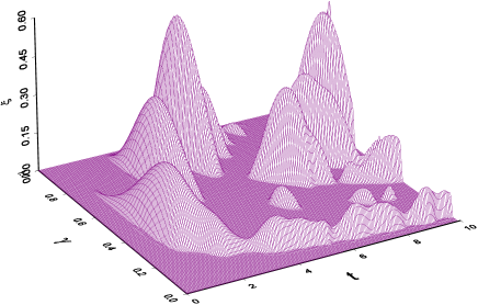
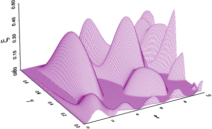
Figure 1: Atom-atom entanglement induced by the interaction with a thermal field having $\bar{n}=1$ when the atoms are initially prepared in $|e_{1},e_{2}\rangle$ (a) and $|e_{1},g_{2}\rangle$ (b).

The dynamical density matrix of the whole system can be obtained by substituting (25)–(42) into (17) and then carrying out the integration with respect to $\phi$. This treatment provides the exact solution of the problem. Moreover, it is easier and better than solving the Liouville equation numerically lee1 . To evaluate the density matrix of the two qubits, i.e. $\hat{\rho}_{a}(t)$, one has to trace over the field variables the density matrix of the system as:

$$\hat{\rho}_{a}(t)=B_{e_{1}e_{2}}|e_{1},e_{2}\rangle\langle e_{1},e_{2}|+B_{g_{1}g_{2}}|g_{1},g_{2}\rangle\langle g_{1},g_{2}|+(B_{e_{1}g_{2}}|e_{1},g_{2}\rangle+B_{g_{1}e_{2}}|g_{1},e_{2}\rangle)(\langle e_{1},g_{2}|B^{*}_{e_{1}g_{2}}+\langle g_{1},e_{2}|B^{*}_{g_{1}e_{2}}),$$ (43)

where

$$\begin{array}[]{lr}B_{e_{1}e_{2}}=\sum\limits_{n=0}^{\infty}P(n)\left[|X_{1}^{(1)}(t,n)|^{2}\sin^{2}\theta\cos^{2}\vartheta+|X_{1}^{(2)}(t,n)|^{2}\sin^{2}\theta\sin^{2}\vartheta+|X_{1}^{(3)}(t,n)|^{2}\cos^{2}\theta\right],\\ B_{g_{1}g_{2}}=\sum\limits_{n=0}^{\infty}P(n)\left[|X_{4}^{(1)}(t,n)|^{2}\sin^{2}\theta\cos^{2}\vartheta+|X_{4}^{(2)}(t,n)|^{2}\sin^{2}\theta\sin^{2}\vartheta+|X_{4}^{(3)}(t,n)|^{2}\cos^{2}\theta\right],\\ B_{e_{1}g_{2}}=\sum\limits_{n=0}^{\infty}P(n)\left[X_{2}^{(1)}(t,n)X_{3}^{(1)*}(t,n)\sin^{2}\theta\cos^{2}\vartheta\right.\\ +\left.X_{2}^{(2)}(t,n)X_{3}^{(2)*}(t,n)\sin^{2}\theta\sin^{2}\vartheta+X_{2}^{(3)}(t,n)X_{3}^{(3)*}(t,n)\cos^{2}\theta\right],\quad B_{g_{1}e_{2}}=B_{e_{1}g_{2}}^{*}.\end{array}$$ (48)

For the best of our knowledge this is the first time the explicit form of the density matrix of this system to be presented. This reflects the power of the approach. The density matrix (43) tends to that of the symmetric case lee2 , which was obtained by the Kraus representation, by simply setting $\lambda_{1}=\lambda_{2}=\lambda$.

To verify the validity of the approach we comment on the entanglement of the two qubits controlled by (43).

In this regard, we use the negative values of the partial transposition lee , which is frequently used for such systems amesen ; lee2 , and is defined as:

$$\xi=-2\sum_{j}\gamma_{j}^{-},$$ (49)

where $\gamma_{j}^{-}$ are the negative eigenvalues of the partial transposition of $\hat{\rho}_{a}(t)$. The entanglement measure ranges between $\xi=0$ for separable qubits and $\xi=1$ for maximally entangled qubits. For the density matrix (43) there is only one eigenvalue of those of the partial transposition matrix, which can approach negative values, having the form:

$$2\gamma_{j}^{-}=B_{e_{1}e_{2}}+B_{g_{1}g_{2}}-\sqrt{(B_{e_{1}e_{2}}-B_{g_{1}g_{2}})^{2}+4|B_{g_{1}e_{2}}|^{2}}.$$ (50)

By means of (38)–(50) we have obtained the results of lee2 for the same values of the interaction parameters. Now it is therefore reasonable to make a comparison with the results of the general case, which has been numerically presented in lee1 . In that article the analysis has been confined to such forms of the coupling constants $\lambda_{1}=1+\gamma$ and $\lambda_{2}=1-\gamma$, where $\gamma$ (with $0\leq\gamma\leq 1$) is the relative difference between the two atomic couplings. This means that the strength of the interaction of one of the bipartites (atom-field) is increasing, while the other is decreasing simultaneously. As an example, in Figs. 1 we plot the quantity $\xi$ for the same values of the interaction parameters as those of Figs. 2 in lee1 , which were given for the concurrence. It is obvious that our figures and those in lee1 are identical even though they represent different measures. This clearly confirm the validity of the approach. Obviously, the analytical treatments are in general better than the numerical ones as they can provide us some analytical facts about the system. For instance, the condition of involving the expression (50) negative values is:

$$\Upsilon=B_{e_{1}e_{2}}B_{g_{1}g_{2}}-|B_{g_{1}e_{2}}|^{2}<0.$$ (51)

From (38)–(48), when $n=0$ and the two atoms are in $|e_{1},g_{2}\rangle$, the inequality (51) can be simplified as:

$$\Upsilon=-\frac{\lambda_{1}\lambda_{2}}{(\lambda_{1}^{2}+\lambda_{2}^{2})^{2}}[\cos(t\Omega^{+}_{-1})-1][\lambda_{1}^{2}\cos(t\Omega^{+}_{-1})+\lambda_{2}^{2}]<0.$$ (52)

It is evident that the expression (52) gives $\Upsilon=\sin^{2}(t\Omega^{+}_{-1})/4$ for the symmetric case. This means that the symmetric case (with $\bar{n}=0$) cannot generate any entanglement between the two atoms, which are initially in $|e_{1},g_{2}\rangle$. Nevertheless, the asymmetric case can generate entanglement for certain values of the coupling constants, in particular, for those satisfying the inequality $\cos(t\Omega^{+}_{-1})<-\lambda_{2}^{2}/\lambda_{1}^{2}$. Furthermore, for the atoms, which are initially in $|g_{1},g_{2}\rangle$ and $n=0$, one can easily prove that $X_{j}^{(3)}(t,0)=0$. Thus, the condition (51) is not fulfilled, i.e. entanglement cannot be established in this case.

It is worth prompting that we have aimed by the above discussion to justify the validity of the approach not to repeat the study of the entanglement of the two qubits. So that we have selected few cases for the sake of comparison only. Nevertheless, from the treatment we have performed, which was not presented here for the sake of brevity, and the other treatments given in amesen ; lee1 ; lee2 we can conclude that a highly chaotic state in an infinite-dimensional Hilbert space can entangle two qubits depending on the type of their interaction with the field as well as the initial conditions of the system. The amounts of entanglement generated by the asymmetric case are much greater than those generated by the symmetric one.

In conclusion, we have developed, for the first time, a simple analytical approach for solving unitary system when the initial field, as one of its components, is in the mixed state, e.g. thermal light. The approach is applicable only when the Schrödinger’s equation of the system is solvable for any initial arbitrary state. We have verified the validity of the approach for some selective cases for the entanglement of two qubits. The approach enables us to check the results, which have been numerically obtained earlier lee1 . As a final note, we believe that our approach represents a powerful tool to solve such type of problems and may impact other applications in the quantum theory.

References

• (1) S. M. Barnett, P. M. Radmore, Methodes in Theoretical Quantum Optics, Oxford University Press, Oxford, 1997.
• (2) A. Vourdas, Phys. Rev. A 34 (1986) 3466; M. S. Kim, F. A. M. de Oliveira, P. L. Knight, Phys. Rev. A 40 (1989) 2494; P. Marian, Phys. Rev. A 45 (1992) 2044; P. Marian, T. A. Marian, Phys. Rev. A 47 (1993) 4474; H. M. Zaid, Y. Ben-Aryeh, Phys. Rev. A 57 (1998) 1451; F. A. A. El-Orany, J. Peřina, M. S. Abdalla, J. Mod. Opt. 46 (1999) 1621.
• (3) M.C. Amesen, S. Bose, V. Vedral, Phys. Rev. Lett. 87 (2001) 017901; M.B. Plenio, S.F. Huelga, Phys. Rev. Lett. 88 (2002) 197901; S. Bose, I. Fuentes-Guridi, P.L. Knight, V. Verdal, Phys. Rev. Lett. 87 (2001) 050401; L. Zhou, H.S. Song, C. Li, J. Opt. B: Quant. Semiclass. Opt. 4 (2002) 425; X.X. Yi, L. Zhou, H.S. Song, J. Phys. A: Math. Gen. 37 (2004) 5477; L.S. Aguiar, P.P. Munhoz, A. Vidiella-Barranco, J. A. Roversi, J. Opt. B: Quant. Semiclass. Opt. 7 (2005) S769; X.-Y. Wang, X.-S. Chen, J. Phys. B: At. Mol. Opt. Phys. 39 (2006) 3805.
• (4) L. Zhou, X.X. Yi, H. S. Song, Y.Q. Quo, J. Opt. B: Quant. Semiclass. Opt. 6 (2004) 378.
• (5) M. S. Kim, J. Lee, D. Ahn, P.L. Knight, Phys. Rev. A 65 (2002) 040101(R).
• (6) S. B. Zheng, G.C. Guo, Phys. Rev. A 63 (2001) 044302; M. Plenio, Phys. Rev. A 59 (1999) 2468; S.-B. Li, J.-B. Xu, Chin. Phys. Lett. 20 (2003) 985.
• (7) M. Nielsen, I. Chuang, Quantum Computation and Quantum Information, Cambridge University Press, Cambridge, England, 2000.
• (8) L. M. Duan, A. Kuzmich, H. J. Kimble, Phys. Rev. A 67 (2003) 032305.
• (9) M.S. Iqbal, S. Mahmood, M.S.K. Razmi, M.S. Zubairy, J. Opt. Soc. Am. B 5 (1988) 1312; M.P. Sharma, D. A. Cardimona, A. Gavrielides, J. Opt. Soc. Am. B 6 (1989) 1942; I. Jex, M. Matsuoko, M. Koashi, Quant. Opt. 5 (1993) 275; I. Jex, Quant. Opt. 2 (1990) 443; F.A.A. El-Orany, J. Phys. A: Math. Gen. 39 (2006) 3397.
• (10) A. Peres, Phys. Rev. Lett. 77 (1996) 1413; M. Horodecki, P. Horodecki, R. Horodecki, Phys. Lett. A 223 (1996) 1; J. Lee, M.S. Kim, Phys. Rev. Lett. 84 (2000) 4236; J. Lee, M.S. Kim, Y.J. Park, and S. Lee, J. Mod. Opt. 47 (2000) 2151.