Optical Spectral Singularities as Threshold Resonances

Abstract

Spectral singularities are among generic mathematical features of complex scattering potentials. Physically they correspond to scattering states that behave like zero-width resonances. For a simple optical system, we show that a spectral singularity appears whenever the gain coefficient coincides with its threshold value and other parameters of the system are selected properly. We explore a concrete realization of spectral singularities for a typical semiconductor gain medium and propose a method of constructing a tunable laser that operates at threshold gain.

Pacs numbers: 03.65.Nk, 42.25.Bs, 42.60.Da, 24.30.Gd

Consider an infinite planar slab gain medium that is aligned along the $x$-axis and the electromagnetic wave given by $\vec{E}(z,t)=E\>e^{i(\mathfrak{K}z-\omega t)}\hat{e}_{x}$, where $E$ is a constant, $\mathfrak{K}$ is the propagation constant, and $\hat{e}_{x}$ stands for the unit vector pointing along the positive $x$-axis. It is easy to show that while traveling through the gain medium the wave is amplified by a factor of $e^{gL}$, where $L$ is the width of the gain medium and $g$ is the gain coefficient. The latter is related to the imaginary part $\kappa$ of the the complex refractive index of the medium,

$$\mathfrak{n}=\eta+i\kappa,$$ (1)

and the wavelength $\lambda:=2\pi c/\omega$ according to silfvast :

$$g=-\frac{4\pi\kappa}{\lambda}.$$ (2)

Often, one places the gain medium between two mirrors to produce a (Fabry-Perot) resonator. This extends the length of the path of the wave through the gain medium and yields a much larger amplification of the wave for the resonance frequencies of the resonator.

In prl-2009 ; pra-2009b , we have outlined an alternative amplification effect that does not involve mirrors. For the system we consider, it requires adjusting $L$ and $g$ so that the system supports a spectral singularity. This is a generic mathematical feature of complex scattering potentials ss-math that obstructs the completeness of the eigenfunctions of the corresponding non-Hermitian Hamiltonian operator. Physically, a spectral singularity is the energy of a scattering state that behaves exactly like a zero-width resonance prl-2009 ; zafar-09 ; longhi ; samsonov . In this letter, we first reveal the relationship between spectral singularities and the well-known laser threshold condition silfvast , and then explore the possibility of tuning the wavelength of the spectral singularity by adjusting the pump intensity. This turns the system into a tunable laser that operates at the threshold gain.

It is easy to show that

$$\vec{E}(z,t)=E\>e^{-i\omega t}\psi(z)\hat{e}_{x},~{}~{}~{}\vec{B}(z,t)=-i\omega^{-1}E\>e^{-i\omega t}\psi^{\prime}(z)\hat{e}_{y},$$

is a solution of Maxwell’s equations for the above system provided that $\hat{e}_{y}$ stands for the unit vector along the positive $y$-axis, $\psi$ is a continuously differentiable solution of the time-independent Schrödinger equation:

$$-\psi^{\prime\prime}(z)+v(z)\psi(z)=k^{2}\psi(z),$$ (3)

$k:=\omega/c=2\pi/\lambda$, and $v$ is the complex barrier potential:

$$v(z):=\left\{\begin{array}[]{ccc}k^{2}\hat{\mathfrak{z}}&{\rm for}&|z|<\frac{L}{2},\\ 0&{\rm for}&|z|\geq\frac{L}{2},\end{array}\right.~{}~{}~{}~{}~{}\hat{\mathfrak{z}}:=1-\mathfrak{n}^{2}.$$ (4)

Solving the Schrödinger equation (3) we find

$$\psi(z)=\left\{\begin{array}[]{ccc}A_{-}e^{ikz}+B_{-}e^{-ikz}&{\rm for}&z\leq-\mbox{\small$L/2$}\\ A_{0}e^{i\mathfrak{n}kz}+B_{0}e^{-i\mathfrak{n}kz}&{\rm for}&|z|<\mbox{\small$L/2$}\\ A_{+}e^{ikz}+B_{+}e^{-ikz}&{\rm for}&z\geq\mbox{\small$L/2$},\end{array}\right.$$ (5)

where $k\in\mathbb{R}^{+}$, $A_{-}$ and $B_{-}$ are free complex coefficients and $A_{0},B_{0},A_{+}$ and $B_{+}$ are complex coefficients related to $A_{-}$ and $B_{-}$. For example, $\mbox{\scriptsize$\left(\begin{array}[]{c}A_{+}\\ B_{+}\end{array}\right)$}=\mathbf{M}\mbox{\scriptsize$\left(\begin{array}[]{c}A_{-}\\ B_{-}\end{array}\right)$}$, where

$$\mathbf{M}:=\frac{1}{4\mathfrak{n}}\left(\begin{array}[]{cc}e^{-iLk}f(\mathfrak{n},-\frac{Lk}{2})&2i(\mathfrak{n}^{2}-1)\sin(\mathfrak{n}Lk)\\ -2i(\mathfrak{n}^{2}-1)\sin(\mathfrak{n}Lk)&e^{iLk}f(\mathfrak{n},\frac{Lk}{2})\end{array}\right)$$

is the transfer matrix, and for all $z_{1},z_{2}\in\mathbb{C}$,

$$f(z_{1},z_{2}):=e^{-2iz_{1}z_{2}}(1+z_{1})^{2}-e^{2iz_{1}z_{2}}(1-z_{1})^{2}.$$ (6)

Because $v$ is an even function of $z$, the left and right reflection and transmission amplitudes coincide. They are respectively given by $R=-M_{21}/M_{22}=M_{12}/M_{22}$ and $T=1/M_{22}$, prl-2009 .

The spectral singularities are the $k^{2}$ values for which $M_{22}=0$, prl-2009 , i.e., the real $k$ values satisfying

$$f(\mathfrak{n},\mbox{$\frac{Lk}{2}$})=0.$$ (7)

Because $f$ is a complex-valued function, Eq. (7) is equivalent to a pair of coupled real transcendental equations for three unknown real variables $\,{\rm Re}(\hat{\mathfrak{z}})$, $\,{\rm Im}(\hat{\mathfrak{z}})$ and $\alpha k$. In Ref. pra-2009b , we outline a method of decoupling these equations. Here we give a more direct solution that reveals some previously unknown aspects of the problem.

First, we use (6) to express (7) in the form

$$e^{-2i\mathfrak{n}Lk}-\left(\frac{1-\mathfrak{n}}{1+\mathfrak{n}}\right)^{2}=0.$$ (8)

Noting that the boundaries of the gain region have a reflectivity of

$$\mathcal{R}:=\left(\frac{\mathfrak{n}-1}{\mathfrak{n}+1}\right)^{2},$$ (9)

we can write (8) as $e^{-2iLk\mathfrak{n}}=\mathcal{R}$. Next, we substitute (1) in this equation and use (2) to express its left-hand side in terms of $g$. This gives

$$e^{-2gL}e^{-4iLk\eta}=\mathcal{R}^{2}.$$ (10)

Taking the modulus of both sides of this equation yields

$$e^{-2gL}=|\mathcal{R}|^{2}.$$ (11)

This is precisely the laser threshold condition silfvast . In other words, a spectral singularity and the associated zero-width resonance appear at the threshold gain:

$$g=g_{\rm th}:=\frac{1}{2L}\ln\frac{1}{|\mathcal{R}|^{2}}.$$ (12)

We wish to stress that the threshold condition (11) is only a necessary condition for having a spectral singularity. It is by no means sufficient. A necessary and sufficient condition is Eq. (8) that we can express as

$$kL=-\frac{1}{2i\mathfrak{n}}\ln\mathcal{R}.$$ (13)

A key observation that reveals the discrete nature of spectral singularities is that, as a complex-valued function, $\ln\mathcal{R}$ has infinitely many values; in view of (1) and (9),

$$\ln\mathcal{R}=\ln|\mathcal{R}|+2i\left[\tan^{-1}\left(\frac{2\kappa}{\eta^{2}+\kappa^{2}-1}\right)-\pi m\right],~{}~{}~{}~{}$$ (14)

where $m$ is an arbitrary integer. Using (1) and (9), we also find

$$|\mathcal{R}|=\frac{(\eta-1)^{2}+\kappa^{2}}{(\eta+1)^{2}+\kappa^{2}}.$$ (15)

Because $\eta>0$, this equation implies $|\mathcal{R}|<1$. Furthermore, in view of (12), we have

$$g=g_{\rm th}=\frac{1}{L}\ln\left[\frac{(\eta+1)^{2}+\kappa^{2}}{(\eta-1)^{2}+\kappa^{2}}\right].$$ (16)

Next, we return to Eq. (13). Because $kL$ is real, the imaginary part of the right-hand side of this equation must vanish. This gives

$$\eta\ln|\mathcal{R}|+2\kappa\left[\tan^{-1}\left(\frac{2\kappa}{\eta^{2}+\kappa^{2}-1}\right)-\pi m\right]=0.$$ (17)

Furthermore, we can express (13) as

$$kL=\frac{\ln|\mathcal{R}|}{2\kappa}.$$ (18)

Because $kL>0$ and $|\mathcal{R}|<1$, (18) implies $\kappa<0$. According to (2), this corresponds to the situation that the medium has a positive gain coefficient. This is a remarkable manifestation of the conservation of energy, because whenever we arrange the parameters of the system so that a spectral singularity is generated, the system begins emitting radiation. This can happen only for a gain medium, i.e., when $g>0$. In pra-2009b , we could only demonstrate this graphically. Here we have derived it rigorously.

Eq. (17) determines the location of spectral singularities in the $\eta$-$\kappa$ plane. In view of the inequalities: $\eta>0$, $\kappa<0$, $|\mathcal{R}|<1$, and the fact that $\tan^{-1}$ is an odd function taking values in $\left(-\frac{\pi}{2},\frac{\pi}{2}\right)$, we can satisfy (17) only for $m\geq 0$. It is also instructive to note that solving for $\ln|\mathcal{R}|$ in (17), substituting the result in (18), and using $k=2\pi\nu/c$, we find the following expression for the frequency $\nu$ of the spectral singularity.

$$\nu = \frac{\nu_{{}_{\!\varnothing}}m}{\eta}-\frac{\nu_{{}_{\!\varnothing}}}{\pi\eta}\tan^{-1}\left(\frac{2\kappa}{\eta^{2}+\kappa^{2}-1}\right),$$ (19)

where $\nu_{{}_{\!\varnothing}}:=\frac{c}{2L}$. The first term on the right-hand side of (19) is the usual resonance frequency of a resonator of length $L$ with perfectly reflecting boundaries. It is important to note that because $\kappa$ and $\eta$ are frequency-dependent quantities, there will be certain frequencies for which they satisfy (17). A spectral singularity will arise if and only if at least one of these frequencies coincides with one of the values fulfilling (19). It turns out that if we fix all the physical parameters of the system this can happen only for a single critical frequency, i.e., a particular mode number $m$.

In order to explore this phenomenon suppose that the gain medium is obtained by doping a host medium of refraction index $n_{0}$ and that it is modeled by a two-level atomic system with lower and upper level population densities $N_{l}$ and $N_{u}$, resonance frequency $\omega_{0}$, and damping coefficient $\gamma$. Then its permittivity ($\varepsilon:=\varepsilon_{0}\mathfrak{n}^{2}$) is given by

$$\varepsilon=\varepsilon_{0}\left[n_{0}^{2}-\frac{\omega_{p}^{2}}{\omega^{2}-\omega_{0}^{2}+i\gamma\,\omega}\right],$$ (20)

where $\varepsilon_{0}$ is the permittivity of the vacuum, $\omega_{p}^{2}:=(N_{l}-N_{u})e^{2}/(m\varepsilon_{0})$, and $e$ and $m$ are electron’s charge and mass, respectively silfvast ; yariv-yeh . In view of (1), (2), and (20), we can express $\omega_{p}^{2}$ in terms of the gain coefficient $g_{0}$ at the resonance frequency $\omega_{0}$. Introducing $\lambda_{0}:=2\pi c/\omega_{0}$ and

$$\kappa_{0}:=-\frac{\lambda_{0}g_{0}}{4\pi},$$ (21)

and using

$$\varepsilon/\varepsilon_{0}=\mathfrak{n}^{2}=(\eta+i\kappa)^{2},$$ (22)

and (2), we have

$$\frac{\omega_{p}^{2}}{\omega_{0}^{2}}=\frac{2\gamma\kappa_{0}\sqrt{n_{0}^{2}+\kappa_{0}^{2}}}{\omega_{0}}=-\frac{cg_{0}\gamma}{\omega_{0}^{2}}\sqrt{n_{0}^{2}+\left(\frac{cg_{0}}{2\omega_{0}}\right)^{2}}.$$ (23)

For example for a semiconductor gain medium silfvast with:

$$n_{0}=3.4,~{}\lambda_{0}=1500\,{\rm nm},~{}\frac{\gamma}{\omega_{0}}=0.02,~{}g_{0}=40\,{\rm cm}^{-1},$$ (24)

we have $\kappa_{0}=-4.7747\times 10^{-4}$ and $\frac{\omega_{p}^{2}}{\omega_{0}^{2}}=-6.4935\times 10^{-5}$. Substituting these values in (20) and using (22), we can express $\delta\eta:=\eta-n_{0}$ and $\kappa$ as functions of $\omega$ and use them to plot a parametric curve $C$ representing the dispersion relation (20). See Figure 1. Next, we return to Eq. (17) and consider it as an implicit function for each value of $m$. Figure 1 also shows the graph of these functions for several values of $m$. These are the curves of spectral singularities that we label by $C_{m}$. As seen from Figure 1 for sufficiently large values of $m$ (i.e., $m\geq 1374$), $C_{m}$ intersects $C$ at two points. One of these ($p_{m+}$) has a positive $\delta\eta$ coordinate and corresponds to a frequency $\omega_{m+}$ that is larger than $\omega_{0}$. The other ($p_{m+}$) has a negative $\delta\eta$ and corresponds to a frequency $\omega_{m-}$ that is smaller than $\omega_{0}$. We can compute the coordinates $(\delta\eta_{m\pm},\kappa_{m\pm})$ of $p_{m\pm}$, find $\omega_{m\pm}$ and $k_{m\pm}:=\omega_{m\pm}/c$, and use (18) to determine $L$. This gives rise to a set of values $L_{m\pm}$ for the length of the gain medium that would allow for the existence of a spectral singularity. For the gain medium (24), setting $m=1374$ we find a pair of spectral singularities with extremely close wavelengths to $\lambda_{0}$, namely $\lambda=1499.9$ and $1500.2\,{\rm nm}$. These correspond to $L=303.074$ and $303.133\,\mu{\rm m}$, respectively.

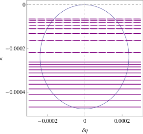
Figure 1: (Color online) Plots of the curves of spectral singularities $C_{m}$ (full and dashed thick purple curves) and the dispersion relation $C$ (thin blue curve) for a gain medium with specifications (24). The spectral label $m$ of the $C_{m}$ that are displayed ranges over $1400,1500,1600,\cdots,2500$ for the thick full (purple) curves from bottom to top, and $3000,4000,5000,\cdots,10000$ for the thick dashed (purple) curves. As one increases $m$ these curves approach to the $\delta\eta$-axis from below. The thin dashed (gray) lines are the coordinate axes.

Next, we consider the more realistic situation that $L$ is fixed and the gain coefficient $g_{0}$ is adjustable. This is simply done by changing the pump intensity. It is not difficult to see that spectral singularities appear for specific discrete values of $g_{0}$ and $\lambda$. This may be viewed as means for producing a tunable laser that would function at the very threshold gain. To implement this idea we insert (23) in (20) and use (22) and $\lambda=2\pi c/\omega$ to express $\delta\eta$ and $\kappa$ as functions of $g_{0}$ and $\lambda$. Substituting the resulting expressions in (17) and (18) and using $k=2\pi/\lambda$ we obtain a pair of equations for $g_{0}$ and $\lambda$ for each value of the mode number $m$. The solution of these equations yield the desired values of $g_{0}$ and $\lambda$ for which a spectral singularity appears.

As we see from Figure 1, the relevant range of values of $\delta\eta$ and $\kappa$ is several orders of magnitude smaller than $n_{0}$. This shows that we can obtain reliable approximate forms of (17) and (18) by neglecting quadratic and higher order terms in $\delta\eta$ and $\kappa$. Applying this approximation to (22) and using (20), we have

$$\delta\eta\approx-\kappa_{0}f_{1},~{}~{}~{}~{}\kappa\approx\kappa_{0}f_{2},$$ (25)

where

$$f_{1}:=\frac{1-\hat{\omega}^{2}}{(1-\hat{\omega}^{2})^{2}+\hat{\gamma}^{2}\hat{\omega}^{2}},~{}~{}f_{2}:=\frac{\hat{\gamma}^{2}\hat{\omega}}{(1-\hat{\omega}^{2})^{2}+\hat{\gamma}^{2}\hat{\omega}^{2}},$$ (26)

$\hat{\omega}:=\omega/\omega_{0}=\lambda_{0}/\lambda$ and $\hat{\gamma}:=\gamma/\omega_{0}$. In view of (25), the above-mentioned approximation scheme is equivalent to neglecting terms of order two and higher in $\kappa_{0}$. Inserting (25) in (18) and using $k=2\pi/\lambda$, we find

$$\kappa_{0}\approx-\frac{\rho_{0}}{2}\left(\frac{f_{1}}{n_{0}^{2}-1}+\frac{\pi L\hat{\omega}f_{2}}{\lambda_{0}}\right)^{-1},$$ (27)

where $\rho_{0}:=\ln[(n_{0}+1)/(n_{0}-1)]$. In light of (21), (27) is equivalent to

$$g_{0}\approx 2\pi\rho_{0}\left(\frac{\lambda_{0}f_{1}}{n_{0}^{2}-1}+\pi L\hat{\omega}f_{2}\right)^{-1}.$$ (28)

Next, we substitute (25) in (18), neglect the quadratic and higher order terms in $\kappa_{0}$, and use (27) and (26) to simplify the result. This yields after some lucky cancelations: $\left(\frac{2\pi Ln_{0}}{\lambda_{0}}-\frac{\rho_{0}}{\hat{\gamma}^{2}}\right)\hat{\omega}^{2}-\pi m\,\hat{\omega}+\frac{\rho_{0}}{\hat{\gamma}^{2}}\approx 0$. Only for $m\geq\mu:=\frac{2\rho_{0}}{\pi\hat{\gamma}}\sqrt{\frac{2\pi Ln_{0}}{\rho_{0}\lambda_{0}}-\frac{1}{\hat{\gamma}^{2}}}$ does this equation have real solutions. These give the frequency (wavelength) of the spectral singularities. Substituting them in (28), we find the corresponding $g_{0}$ values. The approximate values of $\lambda$ and $g_{0}$ obtained in this way allow for a more effective numerical solution of the exact equations (17) and (18).

As a concrete example, we take $L=300~{}\mu{\rm m}$ for the gain medium described by (24) and obtain the wavelength of the spectral singularities that are produced as we change $g_{0}$ in the range $0$ - $115~{}{\rm cm}^{-1}$. These turn out to correspond to the mode numbers $1355$ – $1365$ which are consistent with the result, $m\geq\mu\approx 1320$, of our approximate calculations.The corresponding $\lambda$ and $g_{0}$ values are given in Table 1. The spectral singularity with lowest $g_{0}$ value ($40.4~{}{\rm cm}^{-1}$) has a wavelength that is extremely close to $\lambda_{0}=1500\,{\rm nm}$. It corresponds to $m=1360$. As we increase $g_{0}$ form $40.4$ to $115~{}{\rm cm}^{-1}$, there appear 10 more spectral singularities with wavelengths ranging between $1482$ and $1520\,{\rm nm}$. These should in principle be detectable, if we gradually increase the pump intensity. For example a periodic change of $g_{0}$ in the range $70$ – $90~{}{\rm cm}^{-1}$ should produce periodic emissions of radiation at the wavelengths $\lambda=1484.927\,{\rm nm}$ (for $m=1364$ and $g_{0}=81.6821~{}{\rm cm}^{-1}$) and $\lambda=1515.380\,{\rm nm}$ (for $m=1356$ and $g_{0}=82.4918~{}{\rm cm}^{-1}$) with no emitted wave of comparable amplitude at the resonance wavelength $1500\,{\rm nm}$. This is a remarkable feature of the spectral singularity related resonance effect. Using the above values of $\lambda$ and $g_{0}$ to compute the reflection and transmission coefficients $|R|^{2}$ and $|T|^{2}$, that give the amplification factor for the emitted electromagnetic energy density, we obtain $|R|^{2}\approx|T|^{2}\approx 1.1\times 10^{6}$ and $3.1\times 10^{5}$, respectively. In other words we obtain an amplification of the background electromagnetic energy density at these wavelengths by a factor of $|R|^{2}+|T|^{2}\approx 2.2\times 10^{6}$ and $6.2\times 10^{5}$, respectively. It turns out that these numbers are extremely sensitive to the value of $\lambda$ but not $g_{0}$. Using the less accurate values $81.7$ and $82.5~{}{\rm cm}^{-1}$ for $g_{0}$ and the same values for $\lambda$, we find $|R|^{2}\approx|T|^{2}\approx 1.0\times 10^{6}$ and $2.8\times 10^{5}$. But, as we can see from Figure 2, changing the above values of $\lambda$ by $0.01$ nm reduces $|R|^{2}$ and $|T|^{2}$ by three to four orders of magnitude. This shows that the detection of spectral singularities would require a spectrometer with a band width of $0.01$ nm or smaller.

$m$	$\lambda({\rm nm})$	$g_{0}({\rm cm}^{-1})$	$m$	$\lambda({\rm nm})$	$g_{0}({\rm cm}^{-1})$
1355	1519.832	110.2	1361	1495.662	43.8
1356	1515.380	82.5	1362	1494.582	45.7
1357	1512.058	66.3	1363	1489.203	61.5
1358	1507.651	50.9	1364	1484.927	81.7
1359	1504.363	43.8	1365	1481.736	101.1
1360	1500.000	40.4

Table 1: Wave length $\lambda$ of the spectral singularities for the gain coefficient $g_{0}$ ranging over $0$-$115~{}{\rm cm}^{-1}$ and $L=300~{}\mu{\rm m}$.

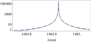
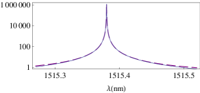
Figure 2: (Color online) Logarithmic plots of the reflection (thick dashed curves) and transmission (thin full curves) coefficients as functions of $\lambda$ for $L=300\,\mu{\rm m}$ and $g=81.7/{\rm cm}$ (top graph) and $g=82.5/{\rm cm}$ (bottom graph).

To summarize, we have explored spectral singularities of a simple optical system and shown that the equation (10) that determines spectral singularities reduces to the laser threshold condition $g=g_{\rm th}$, if we take the modulus of both sides of this equation. Equating the phase of both sides of this equation gives rise to an independent condition for the existence of the spectral singularities that involves an integer (mode) number $m$. It turns out that this equation and the threshold condition can be satisfied only for particular values of the physical parameters of the system and this corresponds to a single value of $m$ and a corresponding critical wavelength. We have also explored the idea of tuning this wavelength by adjusting the pump intensity for a typical semiconductor gain medium. A remarkable feature of the spectral singularity related resonance effect is that if we increase the pump intensity so that the gain exceeds the threshold value, this effect disappears. This marks a clear distinction between the zero-width resonances associated with spectral singularities and the usual resonances that we encounter in optical resonators.

Acknowledgments: I wish to thank Aref Mostafazadeh and Ali Serpenğzel for illuminating discussions. This work has been supported by the Turkish Academy of Sciences (TÜBA).

References

- (1) W. T. Silfvast, Laser Fundamentals, Cambridge University Press, Cambridge, 1996.
- (2) A. Mostafazadeh, Phys. Rev. Lett. 102, 220402 (2009).
- (3) A. Mostafazadeh, Phys. Rev. A 80, 032711 (2009).
- (4) M. A. Naimark, Trudy Moscov. Mat. Obsc. 3, 181 (1954) in Russian, Amer. Math. Soc. Transl. (2), 16, 103 (1960); R. R. D. Kemp, Canadian J. Math. 10, 447 (1958); J. Schwartz, Comm. Pure Appl. Math. 13, 609 (1960); G. Sh. Guseinov, Pramana. J. Phys. 73, 587 (2009).
- (5) Z. Ahmed, J. Phys. A 42, 472005 (2009).
- (6) S. Longhi, Phys. Rev. B 80, 165125 (2009) and Phys. Rev. A 81, 022102 (2010).
- (7) B. F. Samsonov, preprint arXiv:1007.4421.
- (8) A. Yariv and P. Yeh, Photonics, Oxford University Press, Oxford, 2007.