Fractional diffusion equations and processes with randomly varying time

Abstract

In this paper the solutions $u_{\nu}=u_{\nu}(x,t)$ to fractional diffusion equations of order $0<\nu\leq 2$ are analyzed and interpreted as densities of the composition of various types of stochastic processes.

For the fractional equations of order $\nu=\frac{1}{2^{n}}$, $n\geq 1,$ we show that the solutions $u_{{1/2^{n}}}$ correspond to the distribution of the $n$-times iterated Brownian motion. For these processes the distributions of the maximum and of the sojourn time are explicitly given. The case of fractional equations of order $\nu=\frac{2}{3^{n}}$, $n\geq 1,$ is also investigated and related to Brownian motion and processes with densities expressed in terms of Airy functions.

In the general case we show that $u_{\nu}$ coincides with the distribution of Brownian motion with random time or of different processes with a Brownian time. The interplay between the solutions $u_{\nu}$ and stable distributions is also explored. Interesting cases involving the bilateral exponential distribution are obtained in the limit.

TIT1Supported by “Sapienza” University of Rome Grant Ateneo 2007, n. 8.1.1.1.32.

and

60E05, 60G52, 60J65, 33E12, 33C10, Iterated Brownian motion, fractional derivatives, Airy functions, McKean law, Gauss–Laplace random variable, stable distributions

1 Introduction

Time-fractional equations of the form

$$\frac{\partial^{\nu}u}{\partial t^{\nu}}=\lambda^{2}\frac{\partial^{2}u}{\partial x^{2}},\qquad x\in\mathbb{R},t>0,$$ (1)

for $0<\nu\leq 2,$ have been studied by a number of authors since the 1980s: see, for example, Wyss (1986), Nigmatullin (1986), Schneider and Wyss (1989), Mainardi (1995a, 1996) and, more recently, Nigmatullin (2006), Angulo et al. (2000, 2005). Hyperbolic fractional equations similar to (1) have been analyzed, for example, by Engler (1997).

For exhaustive reviews on this topic, also consult Samko, Kilbas and Marichev (1993) and Podlubny (1999).

For interesting applications of fractional equations to physical problems see, for example, Saichev and Zaslavsky (1997), Nigmatullin et al. (2007), Angulo et al. (2005).

Fractional diffusion equations of order $1\leq\nu<2$ emerge in the study of the distribution of the local time of pseudoprocesses related to higher-order heat-type equations; see Beghin and Orsingher (2005).

The time-fractional derivative appearing in (1) must be understood in the sense of Dzerbayshan–Caputo, that is

$$\frac{\partial^{\nu}u}{\partial t^{\nu}}(x,t)$$

$$\qquad=\cases{\displaystyle\frac{1}{\Gamma(m-\nu)}\int_{0}^{t}\frac{1}{(t-s)^{1+\nu-m}}\frac{\partial^{m}u}{\partial t^{m}}(x,s)\,ds,&\quad for $m-1<\nu<m$,\cr\displaystyle\frac{\partial^{m}u}{\partial t^{m}}(x,t),&\quad for $\nu=m$,}$$

where $m-1=\lfloor\nu\rfloor$.

Considering the derivative in the sense of Dzerbayshan–Caputo permits us to study initial value problems for (1) with initial data represented by derivatives of integer order; on this topic, consult Mainardi (1996).

We assume, in particular, the following initial condition:

$$u(x,0)=\delta(x)\qquad\mbox{for }0<\nu\leq 1,$$ (2)

and

$$\cases{u(x,0)=\delta(x),\cr u_{t}(x,0)=0,}\qquad\mbox{for }1<\nu\leq 2.$$ (3)

The general solution to equation (1) subject to (2) or (3) is well known [see Podlubny (1999), formula (4.22), page 142] and reads

$$u_{\nu}(x,t) = \frac{1}{2\lambda t^{\nu/2}}\sum_{k=0}^{\infty}\frac{(-|x|/(\lambda t^{\nu/2}))^{k}}{k!\Gamma(-\nu k/2+1-\nu/2)}$$

$$= \frac{1}{2\lambda t^{\nu/2}}W_{-\nu/2,1-\nu/2}\biggl{(}-\frac{|x|}{\lambda t^{\nu/2}}\biggr{)}$$

where $W_{\alpha,\beta}$ in (1) denotes the so-called Wright function, whose general form is

$$W_{\alpha,\beta}(x)=\sum_{k=0}^{\infty}\frac{x^{k}}{k!\Gamma(\alpha k+\beta)},\qquad\alpha>-1,\beta>0,x\in\mathbb{R}.$$ (5)

Some properties of the Wright function are investigated in Mainardi and Tomirotti (1998) and in Gorenflo, Mainardi and Srivastava (1998). Initial value problems (as well as problems on half-lines with boundary conditions) for equations like (1) are extensively treated and solved in Mainardi (1994, 1995a, 1995b), Gorenflo and Mainardi (1997) and Buckwar and Luchko (1998).

It has been proved also that $u_{\nu}$ is nonnegative and integrates to one for all $0<\nu\leq 2$; see, for example, Orsingher and Beghin (2004).

We present here some alternative forms of the solution $u_{\nu}$ of (1), either as integral functions like

$$u_{\nu}(x,t)=\frac{1}{\pi\nu|x|}\int_{0}^{+\infty}e^{-w}e^{-|x|w^{\nu/2}/(\lambda t^{\nu/2})\cos(\nu\pi/2)}\sin\biggl{(}\frac{|x|w^{\nu/2}}{\lambda t^{\nu/2}}\sin\biggl{(}\frac{\nu\pi}{2}\biggr{)}\biggr{)}\,dw,$$

or in terms of stable densities

$$p_{\alpha}(x;\gamma,\eta)=\frac{1}{2\pi}\int_{-\infty}^{+\infty}e^{-i\beta x}\exp\bigl{\{}-\eta|\beta|^{\alpha}e^{-i\pi\gamma/2\beta/|\beta|}\bigr{\}}\,d\beta,\qquad\alpha\neq 1,$$

as

$$u_{\nu}(x,t)=\cases{\displaystyle\frac{1}{\nu|x|^{2/\nu+1}}p_{\nu/2}\biggl{(}\frac{1}{|x|^{2/\nu}};\frac{\nu}{2},\frac{1}{\lambda t^{\nu/2}}\biggr{)},&\quad$0<\nu\leq 1$,\cr\displaystyle\frac{1}{\nu}p_{2/\nu}\biggl{(}|x|;\frac{2}{\nu}(\nu-1),\lambda^{2/\nu}t\biggr{)},&\quad$1\leq\nu<2$.}$$

In Orsingher and Beghin (2004), we proved that in the special case $\nu=\frac{1}{2},$ the solution (1) coincides with the distribution of the process

$$\mathcal{I}_{1}(t)=B_{1}(|B_{2}(t)|),\qquad t>0,$$ (6)

called the iterated Brownian motion, which consists of a Brownian motion $B_{1}$ whose “time” is an independent reflecting Brownian motion.

In Beghin and Orsingher (2003) we have generalized this result to the case where $\nu=\frac{1}{n},$ $n\in\mathbb{N}$. In this case, for $\lambda^{2}=1/2$, the solution (1) coincides with the distribution of the process

$$J_{1/n}(t)=B_{1}\Biggl{(}\prod_{j=1}^{n-1}G_{j}(t)\Biggr{)},\qquad n>1,t>0,$$ (7)

where the vector process $(G_{1}(t),\ldots,G_{n-1}(t))$ has the following joint distribution:

$$p(w_{1},\ldots,w_{n-1})=\frac{n^{(n-1)/2}}{(2\pi)^{(n-1)/2}\sqrt{t}}e^{-(w_{1}^{n}+\cdots+w_{n-1}^{n})/\sqrt[n-1]{n^{n}t}}w_{2}\cdots w_{n-1}^{n-2},$$

(8)

$$\eqntext{w_{j}\geq 0,1\leq j\leq n-1,}$$ (9)

for $n\geq 2$.

In (7) the role of “time” is played by the product of independent, positive-valued r.v.s, which cannot be identified with well-known distributions as in the special case (6).

In the special case $n=2$, we note that $\emph{J}_{1/2}(t)=\mathcal{I}_{1}(t)$, because (1) becomes the distribution of a reflecting Brownian motion.

We are now able to prove a much stronger result for the case $\nu=\frac{1}{2^{n}}$, $n\in\mathbb{N}$, and for $\lambda^{2}=2^{1/2^{n}-2}$, which has a number of interesting consequences. We will show below that (1) for $\nu=\frac{1}{2^{n}}$ can be written down as

$$\qquad u_{1/2^{n}}(x,t)=2^{n}\int_{0}^{\infty}\cdots\int_{0}^{\infty}\frac{e^{-x^{2}/(2z_{1})}}{\sqrt{2\pi z_{1}}}\frac{e^{-z_{1}^{2}/(2z_{2})}}{\sqrt{2\pi z_{2}}}\cdots\frac{e^{-z_{n}^{2}/(2t)}}{\sqrt{2\pi t}}\,dz_{1}\cdots\,dz_{n}$$ (10)

and this coincides with the distribution of

$$\mathcal{I}_{n}(t)=B_{1}(|B_{2}(|B_{3}(\cdots(|B_{n+1}(t)|)\cdots)|)|),\qquad t>0,$$ (11)

where the $B_{j}$’s are independent Brownian motions.

The iterated Brownian motion $\mathcal{I}$${}_{1}(t)=B_{1}(|B_{2}(t)|)$ has been actively investigated and many of its properties have been obtained by Khoshnevisan and Lewis (1996), Burdzy and San Martìn (1995), Allouba (2002).

The connection between fractional generators of order $1/2$ and the iterated Brownian motion $\mathcal{I}_{1}(t)$ has been studied in Allouba and Zheng (2001) and Baeumer, Meerschaert and Nane (2007). This connection was obtained in Orsingher and Beghin (2004) as a particular case of the analysis of the fractional telegraph equation.

The identity

$$2^{n}\int_{0}^{\infty}\cdots\int_{0}^{\infty}\frac{e^{-x^{2}/(2z_{1})}}{\sqrt{2\pi z_{1}}}\frac{e^{-z_{1}^{2}/(2z_{2})}}{\sqrt{2\pi z_{2}}}\cdots\frac{e^{-z_{n}^{2}/(2t)}}{\sqrt{2\pi t}}\,dz_{1}\cdots dz_{n}$$

(12)

$$\qquad=\frac{1}{(2t)^{1/2^{n+1}}}\sum_{k=0}^{\infty}\frac{(-2|x|/(2t)^{1/2^{n+1}})^{k}}{k!\Gamma(-k/2^{n+1}+1-1/2^{n+1})}$$

shows that there is a deep connection between Wright functions and Gaussian distributions.

For the $n$-times iterated Brownian motion $\mathcal{I}_{n}(t)$, $t>0$, we obtain the distributions of the maximum and the sojourn time (together with the expression of moments) and we work out in detail an explicit form of them for the case of the classical iterated Brownian motion $\mathcal{I}_{1}(t),$ $t>0.$

We note that $\mathcal{I}_{n}(t)$ converges in distribution, for $n\rightarrow+\infty$, to a Gauss–Laplace (or bilateral exponential) random variable, independent from $t>0$.

In Orsingher and Beghin (2004) we have seen that for the fractional telegraph-type equation

$$\cases{\displaystyle\frac{\partial u}{\partial t}+2\lambda\frac{\partial^{1/2}u}{\partial t^{1/2}}=c^{2}\frac{\partial^{2}u}{\partial x^{2}},\cr\displaystyle u(x,0)=\delta(x),}\qquad x\in\mathbb{R},t>0,$$ (13)

the general solution coincides with the distribution of the telegraph process $T$ whose time is an independent reflecting Brownian motion

$$W(t)=T(|B(t)|),\qquad t>0.$$ (14)

We remark that process (14) converges to (7) in the Kac sense (i.e., for $\lambda$, $c\rightarrow\infty$, in such a way that $\frac{c^{2}}{\lambda}\rightarrow 1)$. Related interpretations of the solutions to

$$\cases{\displaystyle\frac{\partial u^{2\nu}}{\partial t^{2\nu}}+2\lambda\frac{\partial^{\nu}u}{\partial t^{\nu}}=c^{2}\frac{\partial^{2}u}{\partial x^{2}},\cr\displaystyle u(x,0)=\delta(x)}$$ (15)

are discussed in Beghin and Orsingher (2003) and Orsingher and Beghin (2004). Generalized forms of the fractional telegraph equation (15) and of its solutions can be found in Saxena, Mathai and Haubold (2006).

We obtain here various types of relationships between the solutions $u_{\nu}$ for different values of $\nu.$ The first one we present is the following:

$$u_{\nu}(x,t)=\frac{1}{\sqrt{\pi t}}\int_{0}^{\infty}e^{-z^{2}/(4t)}u_{2\nu}(x,z)\,dz$$ (16)

(valid for any $0<\nu<1)$, where $u_{2\nu}$ is the solution of (1) with order $2\nu$ instead of $\nu.$ Formula (16) leads, for $\nu=\frac{1}{2^{n}},$ to the $n$-times iterated Brownian motion defined in (11), since it permits us to obtain, in an alternative way, the relationship (10).

In the general case, (16) shows that the process related to the equation (1) of order $\nu$ can be interpreted as the composition of a process governed by the same equation, but with order $2\nu,$ with a Gaussian-distributed time. We also derive the analogous relationship

$$u_{\nu}(x,t)=\int_{0}^{\infty}\frac{1}{\sqrt{4\pi\lambda w}}e^{-x^{2}/(2\lambda w)}\overline{u}_{2\nu}(w,t)\,dw,$$ (17)

where

$$\overline{u}_{2\nu}(w,t)=\cases{2u_{2\nu}(w,t),&\quad$w>0$,\cr 0,&\quad$w<0$.}$$ (18)

Here the roles of space and time are interchanged with respect to (16). Therefore from (17) a further interpretation of the solution emerges, because it coincides with the density of the process

$$B(\mathcal{T}_{\nu}(t)),\qquad t>0,$$

where $B$ is a Brownian motion and $\mathcal{T}_{\nu}(t)$ is a process independent from $B$ with a distribution for each $t$ given in (18).

A relationship similar to (16) and connecting $u_{\nu}$ with $u_{m\nu}$ is established (by applying the multiplication formula of Gamma function) for $m\geq 3$ and $0<\nu\leq 2/m$.

Substantially different situations are encountered for the special cases $\nu=\frac{1}{3},$ $\nu=\frac{2}{3}$ and $\nu=\frac{4}{3}.$ In particular for $\nu=\frac{2}{3}$ we show that the solution to (1) possesses the following simple form:

$$u_{2/3}(x,t)=\frac{3}{2}\frac{1}{\lambda\sqrt[3]{3t}}Ai\biggl{(}\frac{|x|}{\lambda\sqrt[3]{3t}}\biggr{)},$$ (19)

where $Ai(x)$ is the Airy function. The latter emerges as a solution to third-order heat-type equations of the form

$$\frac{\partial u}{\partial t}=-\frac{\partial^{3}u}{\partial x^{3}},\qquad t>0,x\in\mathbb{R}.$$

By using again the relationship (16) we get, for the case $\nu=\frac{1}{3}$, the following result:

$$u_{1/3}(x,t)=\frac{3}{2}\int_{0}^{\infty}\frac{e^{-z^{2}/(4t)}}{\sqrt{\pi t}}\frac{1}{\lambda\sqrt[3]{3z}}Ai\biggl{(}\frac{|x|}{\lambda\sqrt[3]{3z}}\biggr{)}\,dz.$$ (20)

This suggests that we should interpret $u_{1/3}$ as the distribution of

$$J_{1/3}(t)=A(|B(t)|),\qquad t>0,$$

where $A$ is a process whose one-dimensional distribution is given in (19), which coincides with the symmetric stable process of order $1/3$.

Similar relationships seem not to hold for the solutions to fractional equations of order $\nu=\frac{1}{n},n>3$, because the fundamental solutions to

$$\frac{\partial u}{\partial t}=c_{n}\frac{\partial^{n}u}{\partial x^{n}},$$ (21)

$c_{n}=\pm 1$, are sign-varying functions on the whole $x$-axis (while, for $n=3,$ only on the negative half-line), as shown in detail in Lachal (2003). Therefore they cannot be used to construct the functions $u_{\nu}$ emerging from (1), which, for $0<\nu\leq 2$, are nonnegative and integrate to one. We note that the solutions to (21) themselves have been represented as distributions of compositions of artificial processes, which do not display a probabilistic structure [see Funaki (1979), Hochberg and Orsingher (1996), Benanchour, Roynette and Vallois (1999)].

Finally the previous results permit us to establish connections between the solutions $u_{2/3^{n}}$ and $u_{2/3^{n-1}}$. Moreover the explicit form (19) of $u_{2/3}$ suggests that we should interpret them as distributions of processes similar to the $n$-times iterated Brownian motion, but with the role of $B$ replaced by $A$ and the time represented by nested products of the random variables $G_{j}$ defined in (7).

2 Iterated Brownian motions generated by fractional equations

In this section we examine in detail various relationships between solutions to diffusion equations like (1) and processes involving Brownian motion. All results of this section refer to equations of order $0<\nu\leq 1.$

We start with the following general theorem:

Theorem 1.

The solution to

$$\cases{\displaystyle\frac{\partial^{\nu}u}{\partial t^{\nu}}=\lambda^{2}\frac{\partial^{2}u}{\partial x^{2}},\cr u(x,0)=\delta(x),}\qquad x\in\mathbb{R},t>0,$$ (22)

for $0<\nu\leq 1$, can be represented as

$$u_{\nu}(x,t)=\frac{1}{\sqrt{\pi t}}\int_{0}^{\infty}e^{-z^{2}/(4t)}u_{2\nu}(x,z)\,dz$$ (23)

where $u_{2\nu}$ is the solution to

$$\cases{\displaystyle\frac{\partial^{2\nu}u}{\partial z^{2\nu}}=\lambda^{2}\frac{\partial^{2}u}{\partial x^{2}},\cr u(x,0)=\delta(x),}\qquad\mbox{for }0<\nu\leq\frac{1}{2}$$ (24)

or

$$\cases{\displaystyle\frac{\partial^{2\nu}u}{\partial z^{2\nu}}=\lambda^{2}\frac{\partial^{2}u}{\partial x^{2}},\cr u(x,0)=\delta(x),\cr u_{t}(x,0)=0,}\qquad\mbox{for }\frac{1}{2}<\nu\leq 1.$$ (25)

By applying the duplication formula of the Gamma function we have that

$$\Gamma\biggl{(}-\frac{\nu k}{2}+1-\frac{\nu}{2}\biggr{)}=\sqrt{\pi}2^{\nu(k+1)}\frac{\Gamma(1-\nu(k+1))}{\Gamma(1/2(1-\nu(k+1)))}.$$ (26)

By plugging (26) into (1) we get that

$$u_{\nu}(x,t) = \frac{1}{2\lambda t^{\nu/2}}\sum_{k=0}^{\infty}\frac{(-|x|/(\lambda t^{\nu/2}))^{k}\Gamma(1/2(1-\nu(k+1)))}{k!\sqrt{\pi}2^{\nu(k+1)}\Gamma(1-\nu(k+1))}$$

$$= \frac{1}{\sqrt{\pi}2^{\nu+1}\lambda t^{\nu/2}}\sum_{k=0}^{\infty}\frac{(-|x|/(\lambda t^{\nu/2}))^{k}\int_{0}^{\infty}e^{-w}w^{-\nu/2(k+1)-1/2}\,dw}{k!2^{\nu k}\Gamma(1-\nu(k+1))}$$

$$= \frac{1}{\sqrt{\pi}2^{\nu+1}\lambda t^{\nu/2}}\int_{0}^{\infty}e^{-w}w^{-\nu/2-1/2}$$

$$\phantom{\frac{1}{\sqrt{\pi}2^{\nu+1}\lambda t^{\nu/2}}\int_{0}^{\infty}}{}\times\sum_{k=0}^{\infty}\frac{1}{k!\Gamma(1-\nu(k+1))}\biggl{(}-\frac{|x|}{\lambda 2^{\nu}(wt)^{\nu/2}}\biggr{)}^{k}\,dw$$

$$= [\mbox{in view of (\ref{equation2}) with suitable arrangements}]$$

$$= \frac{1}{\sqrt{\pi}2^{\nu}t^{\nu/2}}\int_{0}^{\infty}e^{-w}w^{-\nu/2-1/2}\bigl{(}2\sqrt{tw}\bigr{)}^{\nu}u_{2\nu}\bigl{(}x,2\sqrt{tw}\bigr{)}\,dw$$

$$= \frac{1}{\sqrt{\pi}}\int_{0}^{\infty}e^{-w}w^{-1/2}u_{2\nu}\bigl{(}x,2\sqrt{tw}\bigr{)}\,dw$$

$$= \bigl{[}2\sqrt{tw}=z\bigr{]}$$

$$= \frac{1}{\sqrt{\pi t}}\int_{0}^{\infty}e^{-z^{2}/(4t)}u_{2\nu}(x,z)\,dz$$

and this concludes the proof.

An alternative proof of the relationship (23) is based on the Fourier transforms, since for $u_{\nu}$ the following result is known:

$$\int_{-\infty}^{+\infty}e^{i\beta x}u_{\nu}(x,t)\,dx=E_{\nu,1}(-\beta^{2}\lambda^{2}t^{\nu}),$$

where $E_{\nu,1}(z)=\sum_{k=0}^{\infty}\frac{z^{k}}{\Gamma(k\nu+1)}$ is the Mittag–Leffler function. Taking the Fourier transform of (23) we get that

$$\int_{-\infty}^{+\infty}e^{i\beta x}\biggl{\{}\frac{1}{\sqrt{\pi t}}\int_{0}^{\infty}e^{-w^{2}/(4t)}u_{2\nu}(x,w)\,dw\biggr{\}}\,dx$$

$$\qquad=\frac{1}{\sqrt{\pi t}}\int_{0}^{\infty}e^{-w^{2}/(4t)}E_{2\nu,1}(-\beta^{2}\lambda^{2}w^{2\nu})\,dw$$

$$\qquad=\sum_{k=0}^{\infty}\frac{(-\beta^{2}\lambda^{2})^{k}}{\Gamma(2k\nu+1)}\int_{0}^{\infty}\frac{e^{-w^{2}/(4t)}}{\sqrt{\pi t}}w^{2k\nu}\,dw$$

$$\qquad=\bigl{[}\mbox{for }w=2\sqrt{tz}\bigr{]}$$

$$\qquad=\sum_{k=0}^{\infty}\frac{(-\beta^{2}\lambda^{2})^{k}}{\Gamma(2k\nu+1)}\frac{(2\sqrt{t})^{2k\nu+1}}{2\sqrt{\pi t}}\Gamma\biggl{(}\nu k+\frac{1}{2}\biggr{)}$$

$$\qquad=\sum_{k=0}^{\infty}\frac{(-\beta^{2}\lambda^{2})^{k}}{\Gamma(2k\nu+1)}\frac{(2\sqrt{t})^{2k\nu+1}}{2\sqrt{\pi t}}\sqrt{\pi}2^{1-2\nu k}\frac{\Gamma(2\nu k)}{\Gamma(\nu k)}$$

$$\qquad=\sum_{k=0}^{\infty}\frac{(-\beta^{2}\lambda^{2}t^{\nu})^{k}}{\Gamma(k\nu+1)}=\int_{-\infty}^{+\infty}e^{i\beta x}u_{\nu}(x,t)\,dx.$$

Remark 2.1.

In the special case where $\nu=\frac{1}{2}$, formula (23) yields

$$u_{1/2}(x,t) = \frac{1}{\sqrt{\pi t}}\int_{0}^{\infty}e^{-z^{2}/(4t)}\frac{e^{-x^{2}/(4\lambda^{2}z)}}{\sqrt{4\pi\lambda^{2}z}}\,dz$$

$$= [2\lambda^{2}z=y]$$

$$= \frac{1}{\sqrt{\pi t}}\int_{0}^{\infty}\frac{e^{-x^{2}/(2y)}}{\sqrt{2\pi y}}\frac{e^{-y^{2}/(4t(2\lambda^{2})^{2})}}{2\lambda^{2}}\,dy.$$

Particularly interesting is the case where $2(2\lambda^{2})^{2}=1,$ that is, when $\lambda^{2}=2^{-3/2}$, because (2.1) reduces to

$$u_{1/2}(x,t)=2\int_{0}^{\infty}\frac{e^{-x^{2}/(2y)}}{\sqrt{2\pi y}}\frac{e^{-y^{2}/(2t)}}{\sqrt{2\pi t}}\,dy,$$ (28)

which permits us to conclude that, in this case, the solution coincides with the probability density of the iterated Brownian motion (6).

Remark 2.2.

If we generalize our analysis to the $n$-dimensional case and take $\nu=\frac{1}{2},$ we can show that the process related to a fractional equation of the form

$$\frac{\partial^{1/2}u}{\partial t^{1/2}}=\lambda^{2}\Biggl{\{}\sum_{k=1}^{n}\frac{\partial^{2}u}{\partial x_{k}^{2}}\Biggr{\}},\qquad x_{k}\in\mathbb{R},t>0,$$ (29)

with initial condition

$$u_{1/2}(x_{1},x_{2},\ldots,x_{n},0)=\prod_{k=1}^{n}\delta(x_{k}),$$

has components represented by iterated Brownian motions with a common random time. In other words, the solution to (29) coincides with the distribution of the vector process

$$\cases{B_{1}(|B(t)|),\cr\cdots\cr B_{n}(|B(t)|),}\qquad t>0,$$

where $B_{k},$ $k=1,\ldots,n$, are mutually independent Brownian motions and also independent from $B$.

To check this result we evaluate the Fourier transform of the solution to (29) as follows:

$$\int_{-\infty}^{+\infty}\cdots\int_{-\infty}^{+\infty}e^{i\beta_{1}x_{1}+\cdots+i\beta_{n}x_{n}}u_{1/2}(x_{1},\ldots,x_{n},t)\,dx_{1}\cdots dx_{n}$$

$$\qquad=E_{1/2,1}\Biggl{(}-\lambda^{2}t^{1/2}\Biggl{(}\sum_{k=1}^{n}\beta_{k}^{2}\Biggr{)}\Biggr{)}$$ (30)

$$\qquad=\frac{2}{\sqrt{\pi}}\int_{0}^{\infty}e^{-y^{2}-2y\lambda^{2}t^{1/2}(\sum_{k=1}^{n}\beta_{k}^{2})}\,dy.$$

From (2.2) we get the inverse Fourier transform in the following form:

$$u_{1/2}(x_{1},\ldots,x_{n},t) = \frac{2}{\sqrt{\pi}}\int_{0}^{\infty}e^{-y^{2}}\prod_{k=1}^{n}\frac{e^{-x_{k}^{2}/(2(4t^{1/2}\lambda^{2}y))}}{\sqrt{2\pi(4t^{1/2}\lambda^{2}y)}}\,dy$$

$$= 2\int_{0}^{\infty}\frac{e^{-w^{2}/(2(2^{3}t\lambda^{4}))}}{\sqrt{2\pi(2^{3}t\lambda^{4})}}\prod_{k=1}^{n}\frac{e^{-x_{k}^{2}/(2w)}}{\sqrt{2\pi w}}\,dw.$$

The main difference with respect to the case of the usual multivariate heat equation is that the components of the iterated Brownian motions are no longer independent because they are related to each other by the common random time $B$ (with infinitesimal variance $2^{3}\lambda^{4}t).$

We pass now to our second theorem, which is related to the case $\nu=\frac{1}{2^{n}},$ $n\in\mathbb{N}$.

Theorem 2.

For $\nu=\frac{1}{2^{n}},\lambda=2^{1/2^{(n+1)}-1}$ the solution to equation (1) under the initial condition (2) can be written as

$$\qquad u_{{1/2^{n}}}(x,t)=2^{n}\int_{0}^{\infty}\cdots\int_{0}^{\infty}\frac{e^{-x^{2}/(2z_{1})}}{\sqrt{2\pi z_{1}}}\frac{e^{-z_{1}^{2}/(2z_{2})}}{\sqrt{2\pi z_{2}}}\cdots\frac{e^{-z_{n}^{2}/(2t)}}{\sqrt{2\pi t}}\,dz_{1}\cdots dz_{n}.$$ (31)

In view of the duplication formula for the Gamma function we can write

$$\Gamma\biggl{(}1-\frac{k}{2^{n+1}}-\frac{1}{2^{n+1}}\biggr{)}$$

(32)

$$\qquad=\sqrt{\pi}2^{1/2^{n}+k/2^{n}}\frac{\Gamma(1-k/2^{n}-1/2^{n})}{\Gamma(1/2-k/2^{n+1}-1/2^{n+1})}$$

so that the first member of (1) becomes, for $\nu=\frac{1}{2^{n}}$ and $\lambda=2^{1/2^{(n+1)}-1}$,

$$u_{1/2^{n}}(x,t)$$

$$\qquad=\frac{1}{(2t)^{1/2^{n+1}}}\sum_{k=0}^{\infty}\biggl{(}-\frac{2|x|}{(2t)^{1/2^{n+1}}}\biggr{)}^{k}\frac{1}{k!\Gamma(1-k/2^{n+1}-1/2^{n+1})}$$

$$\qquad=\frac{1}{(2t)^{1/2^{n+1}}}\sum_{k=0}^{\infty}\biggl{(}-\frac{2|x|}{(2t)^{1/2^{n+1}}}\biggr{)}^{k}\frac{\int_{0}^{\infty}e^{-w_{1}}w_{1}^{-1/2^{n+1}-k/2^{n+1}-1/2}\,dw_{1}}{k!\sqrt{\pi}2^{(k+1)/2^{n}}\Gamma(1-k/2^{n}-1/2^{n})}$$

$$\qquad=\frac{1}{(2t)^{1/2^{n+1}}}$$

$$\quad\qquad{}\times\sum_{k=0}^{\infty}\biggl{(}-\frac{2|x|}{(2t)^{1/2^{n+1}}}\biggr{)}^{k}$$ (33)

$$\quad\qquad{}\times\frac{\int_{0}^{\infty}e^{-w_{1}}w_{1}^{-1/2^{n+1}-k/2^{n+1}-1/2}\,dw_{1}\int_{0}^{\infty}e^{-w_{2}}w_{2}^{-1/2^{n}-k/2^{n}-1/2}\,dw_{2}}{k!(\sqrt{\pi})^{2}2^{(k+1)/2^{n}+(k+1)/2^{n-1}}\Gamma(1-k/2^{n-1}-1/2^{n-1})}$$

$$\qquad=\frac{1}{(2t)^{1/2^{n+1}}}$$

$$\quad\qquad{}\times\sum_{k=0}^{\infty}\biggl{(}-\frac{2|x|}{(2t)^{1/2^{n+1}}}\biggr{)}^{k}$$

$$\quad\qquad\phantom{{}\times\sum_{k=0}^{\infty}}{}\times\frac{\int_{0}^{\infty}\int_{0}^{\infty}\cdots\int_{0}^{\infty}e^{-\sum_{j=1}^{n}w_{j}}\prod_{j=1}^{n}w_{j}^{-(k+1)/2^{n+2-j}-1/2}\,dw_{j}}{k!(\sqrt{\pi})^{n}2^{(k+1)\sum_{j=0}^{n-1}1/2^{n-j}}\Gamma(1/2-k/2)}.$$

At this point we can use the reflection formula for the Gamma function

$$\Gamma\biggl{(}\frac{1}{2}-\frac{k}{2}\biggr{)} = \frac{\pi}{\sin\{\pi/2(1-k)\}}\frac{1}{\Gamma((1+k)/2)}$$

$$= \frac{\pi}{\cos k\pi/2\Gamma((1+k)/2)}$$

and this shows that only even terms of (2) must be retained. We can therefore write that

$$u_{1/2^{n}}(x,t)$$

$$\qquad=\frac{1}{(2t)^{1/2^{n+1}}}$$

$$\qquad\quad{}\times\sum_{k=0}^{\infty}\biggl{(}-\frac{2|x|}{(2t)^{1/2^{n+1}}}\biggr{)}^{k}$$

$$\quad\qquad{}\times\Biggl{(}\int_{0}^{\infty}\cdots\int_{0}^{\infty}e^{-\sum_{j=1}^{n}w_{j}}\prod_{j=1}^{n}w_{j}^{-(k+1)/2^{n+2-j}-1/2}\,dw_{j}\Biggr{)}$$

$$\quad\qquad{}\times\cos\frac{k\pi}{2}\Gamma\biggl{(}\frac{1+k}{2}\biggr{)}\bigl{[}k!\bigl{(}\sqrt{\pi}\bigr{)}^{n}\pi 2^{(k+1)\sum_{j=0}^{n-1}1/2^{n-j}}\bigr{]}^{-1}$$

$$\qquad=\frac{2}{(2t)^{1/2^{n+1}}}\sum_{k=0}^{\infty}\biggl{(}-\frac{2|x|}{(2t)^{1/2^{n+1}}}\biggr{)}^{k}$$

$$\quad\qquad{}\times\frac{(\int_{0}^{\infty}\cdots\int_{0}^{\infty}e^{-\sum_{j=1}^{n}w_{j}}\prod_{j=1}^{n}w_{j}^{-(k+1)/2^{n+2-j}-1/2}\,dw_{j})\cos k\pi/2\Gamma(k)}{k!(\sqrt{\pi})^{n+1}2^{\sum_{j=0}^{n-1}1/2^{n-j}}2^{k\sum_{j=0}^{n}1/2^{n-j}}\Gamma(k/2)}$$ (35)

$$\qquad=\frac{2}{(2t)^{1/2^{n+1}}}$$

$$\quad\qquad{}\times\sum_{r=0}^{\infty}\biggl{(}-\frac{2|x|}{(2t)^{1/2^{n+1}}}\biggr{)}^{2r}$$

$$\quad\qquad{}\times\frac{(\int_{0}^{\infty}\cdots\int_{0}^{\infty}e^{-\sum_{j=1}^{n}w_{j}}\prod_{j=1}^{n}w_{j}^{-(2r+1)/2^{n+2-j}-1/2}\,dw_{j})(-1)^{r}}{(\sqrt{\pi})^{n+1}2^{\sum_{j=0}^{n}1/2^{n-j}}2^{2r\sum_{j=0}^{n}1/2^{n-j}}r!}$$

$$\qquad=\frac{2}{(2t)^{1/2^{n+1}}2^{2(1-1/2^{n+1})}(\sqrt{\pi})^{n+1}}$$

$$\quad\qquad{}\times\sum_{r=0}^{\infty}\frac{(-1)^{r}}{r!}\biggl{(}\frac{x^{2}}{t^{1/2^{n}}}2^{2-1/2^{n}}\biggr{)}^{r}\bigl{(}2^{-2(2-1/2^{n})}\bigr{)}^{r}$$

$$\quad\qquad{}\times\Biggl{(}\int_{0}^{\infty}\cdots\int_{0}^{\infty}e^{-\sum_{j=1}^{n}w_{j}}\prod_{j=1}^{n}w_{j}^{-(2r+1)/2^{n+2-j}-1/2}\,dw_{j}\Biggr{)}.$$

By considering that

$$\sum_{r=0}^{\infty}\frac{(-1)^{r}}{r!}\Biggl{[}\frac{x^{2}}{2^{2}}\biggl{(}\frac{2}{t}\biggr{)}^{1/2^{n}}\prod_{j=1}^{n}w_{j}^{-1/2^{n+1-j}}\Biggr{]}^{r}=e^{-x^{2}/2^{2}(2/t)^{1/2^{n}}\prod_{j=1}^{n}w_{j}^{-1/2^{n+1-j}}},$$

we can write (2) as follows:

$$u_{1/2^{n}}(x,t) = \frac{1}{(2t)^{1/2^{n+1}}2^{1-1/2^{n}}(\sqrt{\pi})^{n+1}}$$

$${}\times\int_{0}^{\infty}\cdots\int_{0}^{\infty}e^{-x^{2}/2^{2}(2/t)^{1/2^{n}}\prod_{j=1}^{n}w_{j}^{-1/2^{n+1-j}}}e^{-\sum_{j=1}^{n}w_{j}}$$

$$\phantom{{}\times\int_{0}^{\infty}\cdots\int_{0}^{\infty}}{}\times\prod_{j=1}^{n}\bigl{(}w_{j}^{-1/2^{n+2-j}-1/2}\,dw_{j}\bigr{)}.$$

In order to calculate the integrals let us write

$$2(2^{-1}t)^{1/2^{n}}\prod_{j=1}^{n}w_{j}^{1/2^{n+1-j}}=z_{1}$$

so that

$$w_{n}=\biggl{(}\frac{z_{1}2^{-1}(2^{-1}t)^{-1/2^{n}}}{\prod_{j=1}^{n-1}w_{j}^{1/2^{n+1-j}}}\biggr{)}^{2}$$

and

$$dw_{n}=2z_{1}\,dz_{1}\biggl{(}\frac{2^{-1}(2^{-1}t)^{-1/2^{n}}}{\prod_{j=1}^{n-1}w_{j}^{1/2^{n+1-j}}}\biggr{)}^{2}.$$

Therefore we get

$$u_{1/2^{n}}(x,t) = \frac{1}{(2t)^{1/2^{n+1}}2^{1-1/2^{n}}(\sqrt{\pi})^{n+1}}$$

$${}\times\int_{0}^{\infty}\cdots\int_{0}^{\infty}e^{-x^{2}/(2z_{1})}\prod_{j=1}^{n-1}w_{j}^{-1/2^{n+2-j}-1/2}$$

$$\phantom{{}\times\int_{0}^{\infty}\cdots\int_{0}^{\infty}}{}\times e^{-\sum_{j=1}^{n-1}w_{j}}e^{-z_{1}^{2}/(2^{2}(2^{-1}t)^{1/2^{n-1}}\prod_{j=1}^{n-1}w_{j}^{1/2^{n-j}})}$$

$$\phantom{{}\times\int_{0}^{\infty}\cdots\int_{0}^{\infty}}{}\times 2z_{1}\biggl{(}\frac{2^{-1}(2^{-1}t)^{-1/2^{n}}}{\prod_{j=1}^{n-1}w_{j}^{1/2^{n+1-j}}}\biggr{)}^{2}$$

$$\phantom{{}\times\int_{0}^{\infty}\cdots\int_{0}^{\infty}}{}\times\biggl{(}\frac{z_{1}2^{-1}(2^{-1}t)^{-1/2^{n}}}{\prod_{j=1}^{n-1}w_{j}^{1/2^{n+1-j}}}\biggr{)}^{-1-1/2}\,dz_{1}\,dw_{1}\cdots dw_{n-1}$$

$$= \frac{\sqrt{2}(2^{-1}t)^{-1/2^{n+1}}}{(2t)^{1/2^{n+1}}2^{1-1/2^{n}}(\sqrt{\pi})^{n+1}}$$

$${}\times\int_{0}^{\infty}\frac{e^{-x^{2}/(2z_{1})}}{\sqrt{z_{1}}}\int_{0}^{\infty}\cdots\int_{0}^{\infty}e^{-z_{1}^{2}/(2^{2}(2^{-1}t)^{1/2^{n-1}}\prod_{j=1}^{n-1}w_{j}^{1/2^{n-j}})}$$

$$\phantom{{}\times\int_{0}^{\infty}}{}\times e^{-\sum_{j=1}^{n-1}w_{j}}\prod_{j=1}^{n-1}w_{j}^{-1/2^{n+1-j}-1/2}\,dz_{1}\,dw_{1}\cdots dw_{n-1}.$$

Now we make the similar substitution

$$2(2^{-1}t)^{1/2^{n-1}}\prod_{j=1}^{n-1}w_{j}^{1/2^{n-j}}=z_{2}$$

so that we get again

$$w_{n-1}=\biggl{(}\frac{z_{2}2^{-1}(2^{-1}t)^{-1/2^{n-1}}}{\prod_{j=1}^{n-2}w_{j}^{1/2^{n-j}}}\biggr{)}^{2}$$

and

$$dw_{n-1}=2z_{2}\,dz_{2}\biggl{(}\frac{2^{-1}(2^{-1}t)^{-1/2^{n-1}}}{\prod_{j=1}^{n-2}w_{j}^{1/2^{n-j}}}\biggr{)}^{2}.$$

In view of these substitutions, formula (2) is transformed into

$$u_{1/2^{n}}(x,t)$$

$$\qquad=\frac{\sqrt{2}(2^{-1}t)^{-1/2^{n+1}}\sqrt{2}(2^{-1}t)^{-1/2^{n}}}{(2t)^{1/2^{n+1}}2^{1-1/2^{n}}(\sqrt{\pi})^{n+1}}$$

$$\quad\qquad{}\times\int_{0}^{\infty}\frac{e^{-x^{2}/(2z_{1})}}{\sqrt{z_{1}}}\,dz_{1}\int_{0}^{\infty}\frac{e^{-z_{1}^{2}/(2z_{2})}}{\sqrt{z_{2}}}\,dz_{2}$$ (37)

$$\quad\qquad{}\times\int_{0}^{\infty}\cdots\int_{0}^{\infty}e^{-z_{2}^{2}/(2^{2}(2^{-1}t)^{1/2^{n-2}}\prod_{j=1}^{n-2}w_{j}^{1/2^{n-j-1}})}$$

$$\quad\qquad{}\times\prod_{j=1}^{n-2}w_{j}^{-1/2^{n-j}-1/2}e^{-\sum_{j=1}^{n-2}w_{j}}\,dw_{1}\cdots\,dw_{n-2}.$$

By similar transformations, after $(n-3)$ additional steps, we arrive at

$$u_{1/2^{n}}(x,t) = \frac{\sqrt{2^{n-1}}(2^{-1}t)^{-1/2^{n+1}-1/2^{n}-\cdots-1/2^{3}}}{(2t)^{1/2^{n+1}}2^{1-1/2^{n}}(\sqrt{\pi})^{n+1}}$$

$${}\times\int_{0}^{\infty}\frac{e^{-x^{2}/(2z_{1})}}{\sqrt{z_{1}}}\,dz_{1}\int_{0}^{\infty}\frac{e^{-z_{1}^{2}/(2z_{2})}}{\sqrt{z_{2}}}\,dz_{2}\cdots$$

$${}\times\int_{0}^{\infty}e^{-z_{n-1}^{2}/(2^{2}[(2^{-1}t)^{1/2}w_{1}^{1/2}])}e^{-w_{1}}w_{1}^{-1/2^{2}-1/2}\,dw_{1}.$$

By means of the position

$$2(2^{-1}t)^{1/2}w_{1}^{1/2}=z_{n}$$

we get that

$$w_{1}=(z_{n}2^{-1}(2^{-1}t)^{-1/2})^{2}$$

and

$$dw_{1}=2z_{n}\,dz_{n}(2^{-1}(2^{-1}t)^{-1/2})^{2}.$$

We arrive at the final expression

$$u_{1/2^{n}}(x,t) = \frac{\sqrt{2^{n}}(2^{-1}t)^{-1/2^{n+1}-1/2^{n}-\cdots-1/2^{3}-1/2^{2}}}{(2t)^{1/2^{n+1}}2^{1-1/2^{n}}(\sqrt{\pi})^{n+1}}$$

$${}\times\int_{0}^{\infty}\frac{e^{-x^{2}/(2z_{1})}}{\sqrt{z_{1}}}\,dz_{1}\int_{0}^{\infty}\frac{e^{-z_{1}^{2}/(2z_{2})}}{\sqrt{z_{2}}}\,dz_{2}\cdots$$

$${}\times\int_{0}^{\infty}\frac{e^{-z_{n-1}^{2}/(2z_{n})}}{\sqrt{z_{n}}}e^{-z_{n}^{2}/(2t)}\,dz_{n}$$

$$= \frac{2^{n}}{2^{n/2+1/2}(\sqrt{\pi})^{n+1}\sqrt{t}}$$

$${}\times\int_{0}^{\infty}\frac{e^{-x^{2}/(2z_{1})}}{\sqrt{z_{1}}}\,dz_{1}\cdots\int_{0}^{\infty}\frac{e^{-z_{n-1}^{2}/(2z_{n})}}{\sqrt{z_{n}}}e^{-z_{n}^{2}/(2t)}\,dz_{n},$$

which coincides with (31).

Remark 2.3.

It is well known that the Laplace–Fourier transform of the solution to (1) with initial conditions (2) or (3) is equal, for $0<\nu\leq 2,$ to

$$\qquad\int_{0}^{+\infty}e^{-st}\,ds\int_{-\infty}^{+\infty}e^{i\beta x}u_{\nu}(x,t)\,dx=\frac{s^{\nu-1}}{s^{\nu}+\lambda^{2}\beta^{2}},\qquad s>0,\beta\in\mathbb{R}.$$ (38)

We check that the Laplace–Fourier transform of (31) reduces to (38) for $\nu=\frac{1}{2^{n}}$ and $\lambda^{2}=2^{1/2^{n}-2}$:

$$\int_{-\infty}^{+\infty}e^{i\beta x}u_{1/2^{n}}(x,t)\,dx$$

$$\qquad=2^{n}\int_{-\infty}^{+\infty}e^{i\beta x}\,dx\int_{0}^{\infty}\frac{e^{-x^{2}/(2z_{1})}}{\sqrt{2\pi z_{1}}}\,dz_{1}\cdots\int_{0}^{\infty}\frac{e^{-z_{n}^{2}/(2t)}}{\sqrt{2\pi t}}\,dz_{n}$$

$$\qquad=2^{n}\int_{0}^{\infty}e^{-\beta^{2}/2z_{1}}\frac{e^{-z_{1}^{2}/(2z_{2})}}{\sqrt{2\pi z_{2}}}\,dz_{1}\int_{0}^{\infty}\frac{e^{-z_{2}^{2}/(2z_{3})}}{\sqrt{2\pi z_{3}}}\,dz_{2}\cdots\int_{0}^{\infty}\frac{e^{-z_{n}^{2}/(2t)}}{\sqrt{2\pi t}}\,dz_{n}$$

$$\qquad=2^{n}\sum_{r=0}^{\infty}\biggl{(}-\frac{\beta^{2}}{2}\biggr{)}^{r}\frac{1}{r!}\int_{0}^{\infty}z_{1}^{r}\frac{e^{-z_{1}^{2}/(2z_{2})}}{\sqrt{2\pi z_{2}}}\,dz_{1}\cdots\int_{0}^{\infty}\frac{e^{-z_{n}^{2}/(2t)}}{\sqrt{2\pi t}}\,dz_{n}$$

$$\qquad=2^{n}\sum_{r=0}^{\infty}\biggl{(}-\frac{\beta^{2}}{2}\biggr{)}^{r}\frac{1}{r!}\frac{2^{r/2-1}}{\sqrt{\pi}}\Gamma\biggl{(}\frac{r+1}{2}\biggr{)}$$

$$\quad\qquad\phantom{2^{n}\sum_{r=0}^{\infty}}{}\times\int_{0}^{\infty}z_{2}^{r/2}\frac{e^{-z_{2}^{2}/(2z_{3})}}{\sqrt{2\pi z_{3}}}\,dz_{2}\cdots\int_{0}^{\infty}\frac{e^{-z_{n}^{2}/(2t)}}{\sqrt{2\pi t}}\,dz_{n}$$

$$\qquad=2^{n}\sum_{r=0}^{\infty}\biggl{(}-\frac{\beta^{2}}{2}\biggr{)}^{r}\frac{1}{r!}\frac{2^{r/2-1}2^{r/4-1}}{(\sqrt{\pi})^{2}}\Gamma\biggl{(}\frac{r}{2}+\frac{1}{2}\biggr{)}\Gamma\biggl{(}\frac{r}{4}+\frac{1}{2}\biggr{)}$$

$$\qquad\quad\phantom{2^{n}\sum_{r=0}^{\infty}}{}\times\int_{0}^{\infty}z_{3}^{r/4}\frac{e^{-z_{3}^{2}/(2z_{4})}}{\sqrt{2\pi z_{4}}}\,dz_{3}\cdots\int_{0}^{\infty}\frac{e^{-z_{n}^{2}/(2t)}}{\sqrt{2\pi t}}\,dz_{n}$$

$$\qquad=2^{n}\sum_{r=0}^{\infty}\biggl{(}-\frac{\beta^{2}}{2}\biggr{)}^{r}\frac{1}{r!}\frac{2^{r/2-1}2^{r/4-1}\cdots 2^{r/2^{n-1}-1}}{(\sqrt{\pi})^{n-1}}$$

$$\qquad\quad\phantom{2^{n}\sum_{r=0}^{\infty}}{}\times\Gamma\biggl{(}\frac{r}{2}+\frac{1}{2}\biggr{)}\Gamma\biggl{(}\frac{r}{2^{2}}+\frac{1}{2}\biggr{)}\cdots\Gamma\biggl{(}\frac{r}{2^{n-1}}+\frac{1}{2}\biggr{)}$$

$$\qquad\quad\phantom{2^{n}\sum_{r=0}^{\infty}}{}\times\int_{0}^{\infty}z_{n}^{r/2^{n-1}}\frac{e^{-z_{n}^{2}/(2t)}}{\sqrt{2\pi t}}\,dz_{n}$$

$$\qquad=2^{n}\sum_{r=0}^{\infty}\biggl{(}-\frac{\beta^{2}}{2}\biggr{)}^{r}\frac{1}{r!}\frac{2^{r/2+r/4+\cdots+r/2^{n}-n}}{(\sqrt{\pi})^{n}}t^{r/2^{n}}$$

$$\qquad\quad\phantom{2^{n}\sum_{r=0}^{\infty}}{}\times\Gamma\biggl{(}\frac{r}{2}+\frac{1}{2}\biggr{)}\Gamma\biggl{(}\frac{r}{2^{2}}+\frac{1}{2}\biggr{)}\cdots\Gamma\biggl{(}\frac{r}{2^{n}}+\frac{1}{2}\biggr{)}.$$

By applying the duplication formula we get that

$$\Gamma\biggl{(}\frac{r}{2}+\frac{1}{2}\biggr{)}\Gamma\biggl{(}\frac{r}{2^{2}}+\frac{1}{2}\biggr{)}\cdots\Gamma\biggl{(}\frac{r}{2^{n}}+\frac{1}{2}\biggr{)}$$

$$\qquad=\sqrt{\pi}2^{1-r}\frac{\Gamma(r)}{\Gamma(r/2)}\sqrt{\pi}2^{1-r/2}\frac{\Gamma(r/2)}{\Gamma(r/2^{2})}\cdots\sqrt{\pi}2^{1-r/2^{n-1}}\frac{\Gamma(r/2^{n-1})}{\Gamma(r/2^{n})}$$ (39)

$$\qquad=\sqrt{\pi^{n}}2^{n-r-r/2-\cdots-r/2^{n-1}}\frac{\Gamma(r)}{\Gamma(r/2^{n})}$$

and thus

$$\int_{-\infty}^{+\infty}e^{i\beta x}u_{1/2^{n}}(x,t)\,dx$$

$$\qquad=2^{n}\sum_{r=0}^{\infty}\biggl{(}-\frac{\beta^{2}}{2}\biggr{)}^{r}\frac{1}{r!}2^{r/2+r/4+\cdots+r/2^{n}-n}2^{n-r-r/2-\cdots-r/2^{n-1}}t^{r/2^{n}}\frac{\Gamma(r)}{\Gamma(r/2^{n})}\!\!\!\!\!\!\!\!$$

$$\qquad=\sum_{r=0}^{\infty}\biggl{(}-\frac{\beta^{2}}{2}\biggr{)}^{r}\frac{2^{r/2^{n}-r}t^{r/2^{n}}}{r/2^{n}\Gamma(r/2^{n})}$$

$$\qquad=\sum_{r=0}^{\infty}\biggl{(}-\frac{\beta^{2}t^{1/2^{n}}}{2^{2-1/2^{n}}}\biggr{)}^{r}\frac{1}{\Gamma(r/2^{n}+1)}$$

$$\qquad=E_{1/2^{n},1}\biggl{(}-\frac{\beta^{2}t^{1/2^{n}}}{2^{2-1/2^{n}}}\biggr{)}.$$

By taking the Laplace transform of (2.3) we get

$$\int_{0}^{+\infty}e^{-st}E_{1/2^{n},1}\biggl{(}-\frac{\beta^{2}t^{1/2^{n}}}{2^{2-1/2^{n}}}\biggr{)}\,dt=\frac{s^{1/2^{n}-1}2^{2-1/2^{n}}}{\beta^{2}+2^{2-1/2^{n}}s^{1/2^{n}}},$$

which coincides with (38), for $\nu=\frac{1}{2^{n}}$ and $\lambda^{2}=2^{1/2^{n}-2}$.

The form (31) of the solution $u_{1/2^{n}}$ shows that it coincides with the distribution of the $n$-times iterated Brownian motion defined in (11).

Another representation of the solution to the fractional equation (1) can be inferred from the following result:

Theorem 3.

The solution $u_{\nu}(x,t)=u_{\nu}$ to the initial value problem (22), for $0<\nu\leq 1$, can be written as

$$u_{\nu}(x,t)=\int_{0}^{\infty}\frac{1}{\sqrt{4\pi w\lambda}}e^{-x^{2}/(4w\lambda)}\overline{u}_{2\nu}(w,t)\,dw,$$ (41)

where

$$\overline{u}_{2\nu}(w,t)=\cases{2u_{2\nu}(w,t),&\quad for $w\geq 0$,\cr 0,&\quad for $w<0$}$$ (42)

and $u_{2\nu}$ is the solution of (24) or (25).

We first note that for the solutions to (24) or (25) the following result holds:

$$L(x,s)=\int_{0}^{\infty}e^{-st}u_{2\nu}(x,t)\,dt=\frac{s^{\nu-1}}{2\lambda}e^{-|x|s^{\nu}/\lambda},$$ (43)

as can be obtained by taking the Laplace transform of $\frac{\partial^{2\nu}u}{\partial t^{2\nu}}=\lambda^{2}\frac{\partial^{2}u}{\partial x^{2}}.$ The solution to the corresponding equation

$$s^{2\nu}L-s^{2\nu-1}\delta(x)=\lambda^{2}\frac{d^{2}L}{dx^{2}}$$

coincides with the solution to

$$\cases{\lambda^{2}\dfrac{d^{2}L}{dx^{2}}=s^{2\nu}L,&\quad$x\neq 0$,\cr\dfrac{dL}{dx}\Bigm{|}^{+}-\dfrac{dL}{dx}\Bigm{|}^{-}=-\dfrac{s^{2\nu-1}}{\lambda^{2}},\cr L(s,0^{+})=L(s,0^{-}),}$$

and easily yields (43); see also (3.3) of Orsingher and Beghin (2004). Therefore, by taking the Laplace transform of (41), we get

$$\int_{0}^{\infty}\frac{1}{\sqrt{4\pi w\lambda}}e^{-x^{2}/(4w\lambda)}\biggl{\{}2\int_{0}^{\infty}e^{-st}u_{2\nu}(w,t)\,dt\biggr{\}}\,dw$$

$$\qquad=2\int_{0}^{\infty}\frac{1}{\sqrt{4\pi w\lambda}}e^{-x^{2}/(4w\lambda)}\frac{s^{\nu-1}}{2\lambda}e^{-s^{\nu}/\lambda w}\,dw$$

$$\qquad=[2w=z]$$

$$\qquad=\frac{s^{\nu-1}}{2\lambda}\int_{0}^{\infty}\frac{1}{\sqrt{2\pi z\lambda}}e^{-x^{2}/(2z\lambda)}e^{-s^{\nu}/\lambda z/2}\,dz$$

$$\qquad=\frac{s^{\nu/2-1}}{2\lambda}e^{-|x|s^{\nu/2}/\lambda}$$

and this coincides with the Laplace transform of $u_{\nu}(x,t)$.

Remark 2.4.

Formula (41) suggests that we should represent the solution of (22) as the distribution of the process

$$B(\mathcal{T}_{2\nu}(t)),\qquad t>0,$$ (44)

where $B$ is a Brownian motion with infinitesimal variance $2\lambda$ and $\mathcal{T}_{2\nu}(t)$, $t>0$, is a process, independent from $B,$ with law equal to (42).

It is straightforward that, for $\nu=1/2$, the process (44) coincides with the iterated Brownian motion $\mathcal{I}$₁; see (6).

By comparing the relationship (41) with (23) we note also that, in the composition of processes, Brownian motion plays in the second case the role of “time,” while in the first one it represents “space.”

3 On moments and functionals of the iterated Brownian motion

Some properties of the classical iterated Brownian motion have been obtained by several authors and include the law of iterated logarithm [Burdzy and San Martìn (1995)] and the modulus of continuity [Khoshnevisan and Lewis (1996)]. Applications of the iterated Brownian motion to diffusion in cracks are dealt with in De Blassie (2004).

We start by presenting the distribution of the maximum of the $n$-times iterated Brownian motion and, in an explicit form, for the usual iterated Brownian motion.

Theorem 4.

For the $n$-times iterated Brownian motion

$$\mathcal{I}_{n}(t)=B_{1}(|B_{2}(|B_{3}(\cdots(|B_{n+1}(t)|)\cdots)|)|),\qquad t>0,$$

where $B_{j}$, $j=1,\ldots,n+1$, are independent Brownian motions, we have for $\beta>0$ that

$$\Pr\biggl{\{}\max_{0\leq s\leq t}\mathcal{I}_{n}(s)\in d\beta\biggr{\}}$$

$$\qquad=2\int_{0}^{+\infty}\cdots\int_{0}^{+\infty}\Pr\{B_{1}(y_{1})\in d\beta\}\Pr\biggl{\{}\max_{0\leq z_{1}\leq y_{2}}|B_{2}(z_{1})|\in dy_{1}\biggr{\}}$$ (45)

$$\quad\qquad{}\times\Pr\biggl{\{}\max_{0\leq z_{2}\leq y_{3}}|B_{3}(z_{2})|\in dy_{2}\biggr{\}}\cdots\Pr\biggl{\{}\max_{0\leq z_{n}\leq t}|\emph{B}_{n+1}(z_{n})|\in dy_{n}\biggr{\}}.$$

For $\mathcal{I}_{1}(t)=B_{1}(|B_{2}(t)|)$ we can write that

$$\Pr\biggl{\{}\max_{0\leq s\leq t}\mathcal{I}_{1}(s)\in d\beta\biggr{\}}$$

$$\qquad=\Pr\biggl{\{}\max_{0\leq z\leq\max_{0\leq w\leq t}|B_{2}(w)|}B_{1}(z)\in d\beta\biggr{\}}$$

$$\qquad=E\biggl{\{}\Pr\biggl{\{}\max_{0\leq z\leq\max_{0\leq w\leq t}|B_{2}(w)|}B_{1}(z)\in d\beta\Bigm{|}\max_{0\leq w\leq t}|B_{2}(w)|\biggr{\}}\biggr{\}}$$ (46)

$$\qquad=\int_{0}^{+\infty}\Pr\biggl{\{}\max_{0\leq z\leq y}B_{1}(z)\in d\beta\biggr{\}}\Pr\biggl{\{}\max_{0\leq w\leq t}|B_{2}(w)|\in dy\biggr{\}}$$

$$\qquad=2\int_{0}^{+\infty}\Pr\{B_{1}(y)\in d\beta\}\Pr\biggl{\{}\max_{0\leq w\leq t}|B_{2}(w)|\in dy\biggr{\}}.$$

For $\mathcal{I}_{n}(t)=B_{1}(|\mathcal{I}_{n-1}(t)|),$ $n\geq 1$, we have analogously that

$$\Pr\biggl{\{}\max_{0\leq s\leq t}\mathcal{I}_{n}(s)\in d\beta\biggr{\}}$$

(47)

$$\qquad=2\int_{0}^{+\infty}\Pr\{B_{1}(y)\in d\beta\}\Pr\biggl{\{}\max_{0\leq w\leq t}|\mathcal{I}_{n-1}(w)|\in dy\biggr{\}}$$

and, by induction, we obtain (4).

Remark 3.1.

In the case $n=1$ we can give an explicit expression for (4) as follows:

$$\Pr\biggl{\{}\max_{0\leq s\leq t}\mathcal{I}_{1}(s)\in d\beta\biggr{\}}$$

$$\qquad=2d\beta\int_{0}^{+\infty}\frac{e^{-\beta^{2}/(2w)}}{\sqrt{2\pi w}}$$

$$\qquad\phantom{=2d\beta\int_{0}^{+\infty}}{}\times\Biggl{\{}\sum_{k=-\infty}^{+\infty}(-1)^{k}\biggl{[}(1+2k)\frac{e^{-w^{2}/(2t)(1+2k)^{2}}}{\sqrt{2\pi t}}$$

(48)

$$\qquad\quad\hskip 43.0pt\phantom{{}\times\Biggl{\{}\sum_{k=-\infty}^{+\infty}(-1)^{k}\biggl{[}}{}+(1-2k)\frac{e^{-w^{2}/(2t)(1-2k)^{2}}}{\sqrt{2\pi t}}\biggr{]}\Biggr{\}}\,dw$$

$$\qquad=2\sum_{k=-\infty}^{+\infty}(-1)^{k}\biggl{[}\Pr\biggl{\{}\mathcal{I}_{1}\biggl{(}\frac{t}{(1+2k)^{2}}\biggr{)}\in d\beta\biggr{\}}+\Pr\biggl{\{}\mathcal{I}_{1}\biggl{(}\frac{t}{(1-2k)^{2}}\biggr{)}\in d\beta\biggr{\}}\biggr{]}$$

$$\qquad=2d\beta\sum_{k=-\infty}^{+\infty}(-1)^{k}\biggl{[}u_{1/2}\biggl{(}\beta,\frac{t}{(1+2k)^{2}}\biggr{)}+u_{1/2}\biggl{(}\beta,\frac{t}{(1-2k)^{2}}\biggr{)}\biggr{]},$$

where $u_{1/2}(x,t)$ is given in (28) and in the first step we applied the well-known result for the maximal distribution of the absolute value of Brownian motion [see Shorack and Wellner (1986), page 34]. The last term of (3.1) shows that the distribution of the maximum of the iterated Brownian motion can be expressed in terms of its probability law $u_{1/2}=u_{1/2}(x,t)$, as in the case of the classical Brownian motion.

In principle we could write explicitly the distribution of the maximum of $\mathcal{I}_{n}(t)$ in terms of $u_{1/2^{n}}$, but this produces a sum of $2^{n}$ terms, each of which has a very entangled structure.

On the basis of the same principles it is possible to write down the distribution of the sojourn time on the positive half-line of the process $\mathcal{I}_{n}(t)=B_{1}(|\mathcal{I}_{n-1}(t)|),$ $t>0,$ $n\geq 1,$ defined as

$$\Gamma_{t}=\int_{0}^{\max_{0\leq w\leq t}|\mathcal{I}_{n-1}(w)|}1_{\{z:B_{1}(z)>0\}}\,dz.$$ (49)

This random variable takes values in $[0,+\infty)$, because during the interval $[0,t)$ the process $|\mathcal{I}_{n-1}|$ (which plays the role of time for $B_{1}$) can span the whole positive real axes.

Theorem 5.

For the process $\mathcal{I}_{n}(t)$, $t>0$, the distribution of $\Gamma_{t}$ reads

$$\Pr\{\Gamma_{t}\in ds\}=ds\int_{s}^{+\infty}\frac{1}{\pi\sqrt{s(z-s)}}\Pr\biggl{\{}\max_{0\leq w\leq t}|\mathcal{I}_{n-1}(w)|\in dz\biggr{\}},$$

(50)

$$\eqntext{0\leq s<\infty.}$$ (51)

The definition of $\Gamma_{t}$ given in (49) implies that

$$\Pr\{\Gamma_{t}\in ds\}$$

$$\qquad=E\Biggl{\{}\Pr\Biggl{\{}\Biggl{[}\int_{0}^{\max_{0\leq w\leq t}|\mathcal{I}_{n-1}(w)|}1_{\{z:B_{1}(z)>0\}}\,dz\Biggr{]}\in ds\biggm{|}\max_{0\leq w\leq t}|\mathcal{I}_{n-1}(w)|\Biggr{\}}\Biggr{\}}\!\!\!\!\!\!\!\!$$ (52)

$$\qquad=\int_{s}^{+\infty}\Pr\{\Gamma_{z}\in ds\}\Pr\biggl{\{}\max_{0\leq w\leq t}|\mathcal{I}_{n-1}(w)|\in dz\biggr{\}}.$$

By inserting the arc-sine law in (3) we get (5).

We can check that (5) integrates to one

$$\int_{0}^{+\infty}\Pr\{\Gamma_{t}\in ds\}$$

$$\qquad=\int_{0}^{+\infty}ds\int_{s}^{+\infty}\frac{1}{\pi\sqrt{s(z-s)}}\Pr\biggl{\{}\max_{0\leq w\leq t}|\mathcal{I}_{n-1}(w)|\in dz\biggr{\}}$$

$$\qquad=\int_{0}^{+\infty}\Pr\biggl{\{}\max_{0\leq w\leq t}|\mathcal{I}_{n-1}(w)|\in dz\biggr{\}}\int_{0}^{z}\frac{ds}{\pi\sqrt{s(z-s)}}=1.$$

Remark 3.2.

For the iterated Brownian motion $\mathcal{I}_{1}(t)=B_{1}(|B_{2}(t)|)$ the distribution of $\Gamma_{t}$ can be written explicitly as follows:

$$\Pr\{\Gamma_{t}\in ds\}$$

$$\qquad=ds\int_{s}^{+\infty}\frac{dz}{\pi\sqrt{s(z-s)}}$$

$$\quad\qquad{}\times\sum_{k=-\infty}^{+\infty}(-1)^{k}\biggl{\{}\frac{e^{-z^{2}/(2t)(1+2k)^{2}}}{\sqrt{2\pi t}}(1+2k)+\frac{e^{-z^{2}/(2t)(1-2k)^{2}}}{\sqrt{2\pi t}}(1-2k)\biggr{\}}$$ (53)

$$\qquad=\frac{ds}{\pi\sqrt{2\pi ts}}\sum_{k=-\infty}^{+\infty}(-1)^{k}\biggl{\{}(1+2k)\int_{s}^{+\infty}\frac{e^{-z^{2}/(2t)(1+2k)^{2}}}{\sqrt{z-s}}\,dz$$

$$\hskip 135.0pt{}+(1-2k)\int_{s}^{+\infty}\frac{e^{-z^{2}/(2t)(1-2k)^{2}}}{\sqrt{z-s}}\,dz\biggr{\}}.$$

By the transformation $z=s(1+x^{2})$ the integrals in (3.2) are converted [for $A=\frac{(1\pm 2k)^{2}}{2t}$] into

$$2s\int_{0}^{+\infty}\frac{e^{-s^{2}A(1+x^{2})^{2}}}{\sqrt{s}}\,dx$$

$$\qquad=2\sqrt{s}e^{-s^{2}A}\int_{0}^{+\infty}e^{-s^{2}A(x^{4}+2x^{2})}\,dx$$

$$\qquad=\sqrt{\frac{s}{2}}e^{-s^{2}A/2}K_{1/4}\biggl{(}\frac{As^{2}}{2}\biggr{)},$$

where, in the last step, we have applied formula 3.469.1 of Gradshteyn and Rhyzik (1994) and $K_{1/4}(x)=\frac{\pi}{\sqrt{2}}[I_{-1/4}(x)-I_{1/4}(x)]$ [by formula 8.485 of Gradshteyn and Rhyzik (1994)]. By $I_{\nu}$ we denote the Bessel function of imaginary argument of order $\nu$, that is, $I_{\nu}(x)=\sum_{k=0}^{+\infty}\frac{(x/2)^{2k+\nu}}{k!\Gamma(k+\nu+1)}$. Therefore we get

$$\Pr\{\Gamma_{t}\in ds\}$$

$$\qquad=\frac{ds}{2\pi\sqrt{\pi t}}\sum_{k=-\infty}^{+\infty}(-1)^{k}\biggl{\{}(1+2k)e^{-s^{2}/(4t)(1+2k)^{2}}K_{1/4}\biggl{(}\frac{s^{2}(1+2k)^{2}}{4t}\biggr{)}$$

$$\hskip 95.0pt\quad\qquad{}+(1-2k)e^{-s^{2}/(4t)(1-2k)^{2}}K_{1/4}\biggl{(}\frac{s^{2}(1-2k)^{2}}{4t}\biggr{)}\biggr{\}}.$$

We now derive the explicit form of the moments of even order of $\mathcal{I}$${}_{n}(t)$.

Theorem 6.

For the process $\mathcal{I}_{n}(t)$, $t>0$, the moments of order $2k$ are given by

$$E\mathcal{I}_{n}^{2k}(t) = \frac{(2k)!}{k!}\frac{2^{n}}{2^{k}}\int_{0}^{\infty}x^{k}\,dx\int_{0}^{\infty}\frac{e^{-x^{2}/(2z_{1})}}{\sqrt{2\pi z_{1}}}\,dz_{1}\cdots\int_{0}^{\infty}\frac{e^{-z_{n-1}^{2}/(2t)}}{\sqrt{2\pi t}}\,dz_{n-1}$$

$$= \frac{2^{k/2^{n}}}{2^{2k}}\frac{(2k)!}{\Gamma(k/2^{n}+1)}t^{k/2^{n}}.$$

The first expression in (6) can be proved by observing that, for $n\geq 1$,

$$E\mathcal{I}_{n}^{2k}(t) = E[B_{1}^{2k}(|B_{2}(|B_{3}(\cdots|B_{n+1}(t)|\cdots)|)|)]$$

$$= \frac{(2k)!}{k!}\frac{1}{2^{k}}E|B_{2}(|B_{3}(\cdots|B_{n+1}(t)|\cdots)|)|^{k}$$

$$= \frac{(2k)!}{k!}\frac{1}{2^{k}}2\int_{0}^{+\infty}x^{k}\Pr\{B_{2}(|B_{3}(\cdots|B_{n+1}(t)|\cdots)|)\in dx\}$$

$$= \frac{(2k)!}{k!}\frac{1}{2^{k}}2\int_{0}^{+\infty}x^{k}\Pr\{\mathcal{I}_{n-1}(t)\in dx\},$$

which coincides with the second line of (6). By performing the integrations in (3) we get the explicit expression of the moments of order $2k$:

$$E\mathcal{I}_{n}^{2k}(t) = \frac{\Gamma(k/2+1/2)\Gamma(k/2^{2}+1/2)\cdots\Gamma(k/2^{n}+1/2)2^{k/2+\cdots+k/2^{n}}t^{k/2^{n}}}{2^{n}\sqrt{\pi^{n}}}$$

$${}\times\frac{(2k)!2^{n}}{k!2^{k}}$$

$$= [\mbox{by (\ref{ast})}]$$

$$= \sqrt{\pi^{n}}2^{n-k-k/2-\cdots-k/2^{n-1}}\frac{\Gamma(k)}{\Gamma(k/2^{n})}\frac{2^{k/2+\cdots+k/2^{n}}t^{k/2^{n}}}{2^{k}\sqrt{\pi^{n}}}\frac{(2k)!}{k!}$$

$$= t^{k/2^{n}}2^{n-2k+k/2^{n}}\frac{(2k)!}{k\Gamma(k/2^{n})}.$$

Remark 3.3.

For $n=0$ formula (6) coincides with the moments $EB^{2k}(t)$, which is as it should be, since $\mathcal{I}$${}_{0}(t)=B(t).$

For $n=1$, the moments of the iterated Brownian motion $\mathcal{I}$${}_{1}(t)=B_{1}(|B_{2}(t)|)$ can be evaluated directly as follows:

$$E\mathcal{I}_{1}^{2k}(t) = EB_{1}^{2k}(|B_{2}(t)|)$$

$$= \frac{(2k)!}{k!}\frac{1}{2^{k}}E|B_{2}(t)|^{k}$$

$$= \frac{(2k)!}{k!}\frac{2}{2^{k}}\int_{0}^{+\infty}x^{k}\frac{e^{-x^{2}/(2t)}}{\sqrt{2\pi t}}\,dx$$

$$= \frac{2^{k/2}}{2^{2k}}\frac{(2k)!}{\Gamma(k/2+1)}t^{k/2},$$

which coincides with (6) for $n=1.$

For any $n\geq 1$ and $k=1$, we obtain the explicit form of the variance

$$\operatorname{var}\mathcal{I}_{n}(t)=\frac{2^{1/2^{n}}t^{1/2^{n}}}{2\Gamma(1/2^{n}+1)},$$

while, for $n=0,$ it is $\operatorname{var}\mathcal{I}_{0}(t)=t$, as expected.

Remark 3.4.

For all $t>0$, the sequence $\mathcal{I}$${}_{n}(t)$ converges in distribution, for $n\rightarrow\infty$, to the Gauss–Laplace exponential random variable and its density is independent from $t.$ From (1) we get that

$$\lim_{n\rightarrow\infty}u_{1/2^{n}}(x,t)=e^{-2|x|},\qquad t>0,x\in\mathbb{R}.$$ (57)

By working on the Fourier transform (2.3) of $u_{1/2^{n}}$ we have the following alternative proof:

$$\qquad\quad\lim_{n\rightarrow\infty}\int_{-\infty}^{+\infty}e^{i\beta x}u_{1/2^{n}}(x,t)\,dx = E_{0,1}\biggl{(}-\frac{\beta^{2}}{2^{2}}\biggr{)}=\sum_{k=0}^{\infty}\biggl{(}-\frac{\beta^{2}}{2^{2}}\biggr{)}^{k}=\frac{2^{2}}{2^{2}+\beta^{2}}.$$ (58)

Formula (58) coincides with the characteristic function of (57). Loosely speaking, this shows that the composition of infinite Brownian motions produces the bilateral exponential distribution.

In view of (10) we have also the identity

$$\lim_{n\rightarrow\infty}2^{n}\int_{0}^{\infty}\cdots\int_{0}^{\infty}\frac{e^{-x^{2}/(2z_{1})}}{\sqrt{2\pi z_{1}}}\frac{e^{-z_{1}^{2}/(2z_{2})}}{\sqrt{2\pi z_{2}}}\cdots\frac{e^{-z_{n}^{2}/(2t)}}{\sqrt{2\pi t}}\,dz_{1}\cdots dz_{n}$$

(59)

$$\qquad=e^{-2|x|},$$

which is a rather striking result. Furthermore, if we assume that

$$\lim_{n\rightarrow\infty}\frac{\partial^{1/2^{n}}u}{\partial t^{1/2^{n}}}=u,$$

the fractional equation (1) is converted into

$$u=\frac{1}{2^{2}}\frac{\partial^{2}u}{\partial x^{2}},$$

subject to

$$u(x,0)=\delta(x),$$

which is satisfied by (57) for all $x\neq 0$.

Remark 3.5.

For the random process

$$T(|B_{2}(|B_{3}(\cdots|B_{n+1}(t)|\cdots)|)|),\qquad t>0,$$ (60)

where $T$ is a telegraph process (with parameters $\lambda$ and $c$) independent from the Brownian motions $B_{k},$ $k=2,\ldots,n+1$, we have a similar result. The distribution $u_{1/2^{n}}$ of (60) is a solution to

$$\cases{\dfrac{\partial^{2/2^{n}}u}{\partial t^{2/2^{n}}}+2\lambda\dfrac{\partial^{1/2^{n}}u}{\partial t^{1/2^{n}}}=c^{2}\dfrac{\partial^{2}u}{\partial x^{2}},\cr u(x,0)=\delta(x),}\qquad x\in\mathbb{R},t>0$$

and its characteristic function is equal to

$$\int_{-\infty}^{+\infty}e^{i\beta x}u_{1/2^{n}}(x,t)\,dx$$

$$\qquad=\frac{1}{2}\biggl{[}\biggl{(}1+\frac{\lambda}{\sqrt{\lambda^{2}-c^{2}\beta^{2}}}\biggr{)}E_{1/2^{n},1}(\eta_{1}t^{1/2^{n}})$$ (61)

$$\hskip 45.0pt{}+\biggl{(}1-\frac{\lambda}{\sqrt{\lambda^{2}-c^{2}\beta^{2}}}\biggr{)}E_{1/2^{n},1}(\eta_{2}t^{1/2^{n}})\biggr{]},$$

where $\eta_{1}=-\lambda+\sqrt{\lambda^{2}-c^{2}\beta^{2}}$ and $\eta_{2}=-\lambda-\sqrt{\lambda^{2}-c^{2}\beta^{2}}$ [see Orsingher and Beghin (2004), formula (2.7), for $\alpha=1/2^{n}$].

For $n\rightarrow\infty$ we get from (3.5) that

$$\lim_{n\rightarrow\infty}\int_{-\infty}^{+\infty}e^{i\beta x}u_{1/2^{n}}(x,t)\,dx=\frac{1+2\lambda}{1+2\lambda+c^{2}\beta^{2}},$$ (62)

which is the characteristic function of the bilateral exponential random variable, with density

$$f(x)=\frac{\sqrt{1+2\lambda}}{2c}e^{-|x|\sqrt{1+2\lambda}/c},\qquad x\in\mathbb{R}.$$ (63)

Clearly, for $\lambda=0$ and $c=1/2$, (63) reduces to (57) and (62) coincides with (58).

4 The explicit solution of the fractional diffusion equation for $\nu=1/3$, $\nu=2/3$ and $\nu=4/3$

In some special cases it is possible to present the solutions of the fractional equations (1) in a more attractive fashion. This is the case for $\nu=\frac{2}{3}$. The explicit form of $u_{2/3}(x,t)$ is given in the next theorem, in terms of Airy functions.

By combining this result with the relationship given in Theorem 1, $u_{1/3}(x,t)$ can be represented consequently in an interesting form.

Theorem 7.

The solution to

$$\cases{\dfrac{\partial^{2/3}u}{\partial t^{2/3}}=\lambda^{2}\dfrac{\partial^{2}u}{\partial x^{2}},\cr u(x,0)=\delta(x),}\qquad x\in\mathbb{R},t>0$$ (64)

can be represented as

$$u_{2/3}(x,t)=\frac{3}{2}\frac{1}{\lambda\sqrt[3]{3t}}Ai\biggl{(}\frac{|x|}{\lambda\sqrt[3]{3t}}\biggr{)},$$ (65)

where

$$Ai(w) = \frac{1}{\pi}\int_{0}^{+\infty}\cos\biggl{(}\alpha w+\frac{\alpha^{3}}{3}\biggr{)}\,d\alpha$$

$$= \frac{w^{1/2}}{3}\biggl{[}I_{-1/3}\biggl{(}\frac{2w^{3/2}}{3}\biggr{)}-I_{1/3}\biggl{(}\frac{2w^{3/2}}{3}\biggr{)}\biggr{]}$$

is the Airy function and $I_{\nu}$ denotes the Bessel function of imaginary argument of order $\nu$.

From (1) we readily have that

$$u_{2/3}(x,t) = \frac{1}{2\lambda t^{1/3}}\sum_{k=0}^{\infty}\frac{(-|x|/(\lambda t^{1/3}))^{k}}{k!\Gamma(1-(k+1)/3)}$$

$$= \frac{1}{2\pi\lambda t^{1/3}}\sum_{k=0}^{\infty}\frac{(-|x|/(\lambda t^{1/3}))^{k}\Gamma((k+1)/3)\sin(\pi(k+1)/3)}{k!}.$$

By direct inspection the following identity is proven to hold:

$$\sin\frac{\pi(k+1)}{3}=(-1)^{k}\sin\frac{2\pi(k+1)}{3}$$ (68)

and, by inserting this into (4), we get that

$$\qquad u_{2/3}(x,t)=\frac{1}{2\pi\lambda t^{1/3}}\sum_{k=0}^{\infty}\frac{(|x|/(\lambda t^{1/3}))^{k}\Gamma((k+1)/3)\sin(2\pi(k+1)/3)}{k!}.$$ (69)

We note that, from (7), for all $|w|<\infty$,

$$Ai(w) = \frac{w^{1/2}}{3}\biggl{[}I_{-1/3}\biggl{(}\frac{2w^{3/2}}{3}\biggr{)}-I_{1/3}\biggl{(}\frac{2w^{3/2}}{3}\biggr{)}\biggr{]}$$

$$= \frac{w^{1/2}}{3}\Biggl{[}\sum_{k=0}^{\infty}\biggl{(}\frac{w^{3/2}}{3}\biggr{)}^{2k-1/3}\frac{1}{k!\Gamma(k-1/3+1)}$$

$$\hskip 28.0pt{}-\sum_{k=0}^{\infty}\biggl{(}\frac{w^{3/2}}{3}\biggr{)}^{2k+1/3}\frac{1}{k!\Gamma(k+1/3+1)}\Biggr{]}$$

$$= \sum_{k=0}^{\infty}\frac{w^{3k}}{3^{2k+2/3}}\frac{1}{k!\Gamma(k+2/3)}-\sum_{k=0}^{\infty}\frac{w^{3k}}{3^{2k+4/3}}\frac{1}{k!\Gamma(k+4/3)}$$

$$= \frac{2}{3^{7/6}}\sum_{k=0}^{\infty}\biggl{(}\frac{w}{3^{2/3}}\biggr{)}^{k}\frac{\sin(2\pi(k+1)/3)}{\Gamma((k+2)/3)\Gamma((k+3)/3)}.$$

The last step can be justified by taking $k=3m,3m+1$ and $3m+2$. While for $k=3m+2$ the last term in (4) is equal to zero, in the other two cases the two series are obtained.

The triplication formula of the Gamma function [see Lebedev (1972), page 14], that is,

$$\Gamma(z)\Gamma\biggl{(}z+\frac{1}{3}\biggr{)}\Gamma\biggl{(}z+\frac{2}{3}\biggr{)}=\frac{2\pi}{3^{3z-1/2}}\Gamma(3z),$$ (71)

for $z=\frac{k+1}{3}$ yields

$$\Gamma\biggl{(}\frac{k+2}{3}\biggr{)}\Gamma\biggl{(}\frac{k+3}{3}\biggr{)}=\frac{2\pi}{3^{k+1/2}}\frac{\Gamma(k+1)}{\Gamma((k+1)/3)}.$$ (72)

From (72) we have that

$$Ai(w)=\frac{3^{-2/3}}{\pi}\sum_{k=0}^{\infty}(3^{1/3}w)^{k}\frac{\sin(2\pi(k+1)/3)}{k!}\Gamma\biggl{(}\frac{k+1}{3}\biggr{)},$$ (73)

and (65) easily follows by comparing (73) and (69).

Remark 4.1.

The expression of $u_{2/3}(x,t)$ obtained in the previous theorem can be recognized (up to the factor $3/2$) as the solution of the third-order heat-type equation

$$\cases{\displaystyle\frac{\partial v}{\partial t}=-\lambda^{3}\frac{\partial^{3}v}{\partial y^{3}},\cr v(y,0)=\delta(y),}\qquad y\in\mathbb{R},t>0,$$ (74)

evaluated at $y=|x|$. Since $Ai(y)$, for $y>0$, is positive-valued [see Figure 1(a)] and the function (65) integrates to one (as we show below), $u_{2/3}(x,t)$ is a true probability distribution:

$$\int_{-\infty}^{+\infty}u_{2/3}(x,t)\,dx$$

$$\qquad=\frac{3}{2}\Biggl{[}\int_{0}^{+\infty}\frac{1}{\lambda\sqrt[3]{3t}}Ai\biggl{(}\frac{x}{\lambda\sqrt[3]{3t}}\biggr{)}\,dx+\int_{-\infty}^{0}\frac{1}{\lambda\sqrt[3]{3t}}Ai\biggl{(}-\frac{x}{\lambda\sqrt[3]{3t}}\biggr{)}\,dx\Biggr{]}$$

$$\qquad=2\frac{3}{2}\int_{0}^{+\infty}Ai(y)\,dy=1,$$

where the last step follows by noting that $\int_{0}^{+\infty}Ai(y)\,dy=1/3$; see Nikitin and Orsingher (2000).

Therefore we can think of $u_{2/3}(x,t)$ as the probability law of a process $A(t),t>0,$ whose distribution at time $t$ is obtained from the solution $v(x,t)$ of equation (74), as follows:

$$u_{2/3}(x,t)=\tfrac{3}{2}v(|x|,t).$$

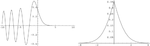
(a)                                                   (b)

Figure 1: The Airy function and the function $Ai(|x|)$.

Remark 4.2.

For the case $\nu=\frac{1}{3}$ the solution $u_{1/3}(x,t)$ to (1) can be written, thanks to the relationship (23), as

$$u_{1/3}(x,t) = \frac{1}{\sqrt{\pi t}}\int_{0}^{\infty}e^{-z^{2}/(4t)}u_{2/3}(x,z)\,dz$$

$$= \frac{1}{\sqrt{\pi t}}\int_{0}^{\infty}e^{-z^{2}/(4t)}\frac{3^{2/3}}{2\lambda z^{1/3}}Ai\biggl{(}\frac{|x|}{\lambda\sqrt[3]{3z}}\biggr{)}\,dz.$$

We can represent (4.2) as the distribution of the process

$$J_{1/3}(t)=A(|B(t)|),\qquad t>0,$$

with $A$ and $B$ independent. The results (65) and (4.2) show that the solutions $u_{2/3}(x,t)$ and $u_{1/3}(x,t)$ are both unimodal with maximum at $x=0$; see Figure 1(b). This is in accordance with the general result that, for $0<\nu\leq 1$, the solutions to the fractional equation (1) have a unique maximal point at $x=0$.

We consider now the case $\nu=4/3$, which is qualitatively different from those dealt with so far, because the solutions of fractional equations of order $1<\nu<2$ display a substantially different behavior.

Theorem 8.

The solution to

$$\cases{\displaystyle\frac{\partial^{4/3}u}{\partial t^{4/3}}=\lambda^{2}\frac{\partial^{2}u}{\partial x^{2}},\cr\displaystyle u(x,0)=\delta(x),\cr\displaystyle u_{t}(x,0)=0,}\qquad x\in\mathbb{R},t>0,$$ (76)

is given by

$$\qquad\quad u_{4/3}(x,t)=\frac{1}{\lambda\sqrt{\pi}}\biggl{(}\frac{3}{4t}\biggr{)}^{2/3}\int_{0}^{+\infty}e^{-w}w^{-1/6}Ai\biggl{(}-\frac{|x|}{\lambda}\biggl{(}\frac{2}{t}\sqrt{\frac{w}{3}}\biggr{)}^{2/3}\biggr{)}\,dw.$$ (77)

From (1) we have that

$$u_{4/3}(x,t) = \frac{1}{2\lambda t^{2/3}}\sum_{k=0}^{\infty}\biggl{(}-\frac{|x|}{\lambda t^{2/3}}\biggr{)}^{k}\frac{1}{k!\Gamma(1-2/3(k+1))}$$

$$= \frac{1}{2\lambda\pi t^{2/3}}\sum_{k=0}^{\infty}\biggl{(}-\frac{|x|}{\lambda t^{2/3}}\biggr{)}^{k}\frac{\Gamma(2/3(k+1))\sin(2\pi(k+1)/3)}{k!}.$$

By means of the duplication formula for the Gamma function we have that

$$\Gamma\biggl{(}\frac{1}{3}(k+1)+\frac{1}{2}\biggr{)}=\frac{\sqrt{\pi}2^{1-2/3(k+1)}\Gamma(2/3(k+1))}{\Gamma((k+1)/3)},$$

and therefore $u_{4/3}(x,t)$ can be rewritten as

$$u_{4/3}(x,t) = \frac{1}{2\lambda\pi\sqrt{\pi}2^{1/3}t^{2/3}}$$

$${}\times\sum_{k=0}^{\infty}\biggl{(}-\frac{2^{2/3}|x|}{\lambda t^{2/3}}\biggr{)}^{k}\frac{\sin(2\pi(k+1)/3)}{k!}\Gamma\biggl{(}\frac{k+1}{3}\biggr{)}\Gamma\biggl{(}\frac{k+1}{3}+\frac{1}{2}\biggr{)}$$

$$= \frac{1}{2\lambda\pi\sqrt{\pi}2^{1/3}t^{2/3}}$$

$${}\times\sum_{k=0}^{\infty}\int_{0}^{+\infty}e^{-w}w^{1/3(k+1)+1/2-1}$$

$$\phantom{{}\times\sum_{k=0}^{\infty}\int_{0}^{+\infty}}{}\times\Gamma\biggl{(}\frac{k+1}{3}\biggr{)}\biggl{(}-\frac{|x|}{\lambda}\biggl{(}\frac{2}{t}\biggr{)}^{2/3}\biggr{)}^{k}\frac{\sin(2\pi(k+1)/3)}{k!}\,dw$$

$$= \frac{1}{2\lambda\pi\sqrt{\pi}2^{1/3}t^{2/3}}$$

$${}\times\sum_{k=0}^{\infty}\int_{0}^{+\infty}e^{-w}w^{1/2-2/3}\biggl{(}-\frac{|x|}{\lambda}\biggl{(}\frac{2}{t}\biggr{)}^{2/3}w^{1/3}\biggr{)}^{k}$$

$$\phantom{{}\times\sum_{k=0}^{\infty}\int_{0}^{+\infty}}{}\times\frac{\sin(2\pi(k+1)/3)}{k!}\Gamma\biggl{(}\frac{k+1}{3}\biggr{)}\,dw$$

$$= [\mbox{by (\ref{tre.11})}]$$

$$= \frac{3^{2/3}}{2\lambda\sqrt{\pi}2^{1/3}t^{2/3}}\int_{0}^{+\infty}e^{-w}w^{-1/6}Ai\biggl{(}-\frac{|x|}{\lambda}\biggl{(}\frac{2}{t}\sqrt{\frac{w}{3}}\biggr{)}^{2/3}\biggr{)}\,dw.$$

We can show that $\int_{-\infty}^{+\infty}u_{4/3}(x,t)\,dx=1$. Indeed, from (77) we have that

$$\frac{1}{\lambda\sqrt{\pi}}\biggl{(}\frac{3}{4t}\biggr{)}^{2/3}\int_{0}^{+\infty}e^{-w}w^{-1/6}\int_{-\infty}^{+\infty}Ai\biggl{(}-\frac{|x|}{\lambda}\biggl{(}\frac{2}{t}\sqrt{\frac{w}{3}}\biggr{)}^{2/3}\biggr{)}\,dx\,dw$$

$$\qquad=\frac{2}{\lambda\sqrt{\pi}}\biggl{(}\frac{3}{4t}\biggr{)}^{2/3}\int_{0}^{+\infty}e^{-w}w^{-1/6}\int_{0}^{+\infty}Ai\biggl{(}-\frac{x}{\lambda}\biggl{(}\frac{2}{t}\sqrt{\frac{w}{3}}\biggr{)}^{2/3}\biggr{)}\,dx\,dw$$

$$\qquad=\biggl{[}\mbox{by the substitution }y=-\frac{x}{\lambda}\biggl{(}\frac{2}{t}\sqrt{\frac{w}{3}}\biggr{)}^{2/3}\biggr{]}$$

$$\qquad=\frac{2}{\lambda\sqrt{\pi}}\biggl{(}\frac{3}{4t}\biggr{)}^{2/3}\lambda\biggl{(}\frac{2}{t}\sqrt{\frac{1}{3}}\biggr{)}^{-2/3}\int_{0}^{+\infty}e^{-w}w^{-1/2}\int_{-\infty}^{0}Ai(y)\,dy\,dw$$

$$\qquad=\frac{1}{\sqrt{\pi}}\frac{2}{3}2\biggl{(}\frac{3}{4}\biggr{)}^{2/3}\frac{2^{-2/3}}{3^{-1/3}}\int_{0}^{+\infty}e^{-w}w^{-1/2}\,dw=1.$$

Remark 4.3.

In view of Theorem 1 we have the following representation for $u_{2/3}(x,t)$, which is alternative to (65):

$$u_{2/3}(x,t) = \frac{1}{\sqrt{\pi t}}\int_{0}^{\infty}e^{-z^{2}/(4t)}u_{4/3}(x,z)\,dz$$

$$= \frac{3^{2/3}}{2\lambda\sqrt{\pi}2^{1/3}}\int_{0}^{+\infty}\frac{e^{-z^{2}/(4t)}}{z^{2/3}\sqrt{\pi t}}\,dz$$

$${}\times\int_{0}^{+\infty}e^{-w}w^{-1/6}Ai\biggl{(}-\frac{|x|}{\lambda}\biggl{(}\frac{2}{z}\sqrt{\frac{w}{3}}\biggr{)}^{2/3}\biggr{)}\,dw.$$

By inserting (65) into the left-hand side of (4.3) we obtain that

$$\frac{3}{2\lambda\sqrt[3]{3t}}Ai\biggl{(}\frac{|x|}{\lambda\sqrt[3]{3t}}\biggr{)}$$

$$\qquad=\frac{3^{2/3}}{2\lambda\sqrt{\pi}2^{1/3}}\int_{0}^{+\infty}\frac{e^{-z^{2}/(4t)}}{\sqrt{\pi t}z^{2/3}}\,dz$$

$$\quad\qquad{}\times\int_{0}^{+\infty}e^{-w}w^{-1/6}Ai\biggl{(}-\frac{|x|}{\lambda}\biggl{(}\frac{2}{z}\sqrt{\frac{w}{3}}\biggr{)}^{2/3}\biggr{)}\,dw$$

$$\qquad=\bigl{[}\mbox{by the substitution }s=\sqrt[3]{2^{2}twz^{-2}}\bigr{]}$$

$$\qquad=\frac{3^{2/3}}{2\lambda\sqrt{\pi}2^{1/3}}\int_{0}^{+\infty}\frac{e^{-z^{2}/(4t)}}{\sqrt{\pi t}z^{2/3}}\frac{3z^{5/3}}{2^{5/3}t^{5/6}}s^{3/2}\,dz$$ (81)

$$\quad\qquad{}\times\int_{0}^{+\infty}e^{-z^{2}s^{3}/(4t)}Ai\biggl{(}-\frac{|x|s}{\lambda\sqrt[3]{3t}}\biggr{)}\,ds$$

$$\qquad=\frac{3^{5/3}}{2^{3}\lambda\pi t^{4/3}}\int_{0}^{+\infty}Ai\biggl{(}-\frac{|x|s}{\lambda\sqrt[3]{3t}}\biggr{)}s^{3/2}\,ds\int_{0}^{+\infty}ze^{-z^{2}(1+s^{3})/(4t)}\,dz$$

$$\qquad=\frac{3^{5/3}}{2^{2}\lambda\pi t^{1/3}}\int_{0}^{+\infty}\frac{s^{3/2}}{1+s^{3}}Ai\biggl{(}-\frac{|x|s}{\lambda\sqrt[3]{3t}}\biggr{)}\,ds$$

$$\qquad=\frac{3^{2/3}}{2\lambda t^{1/3}}\int_{0}^{+\infty}\Pr\{|B(T_{0})|\in ds\}Ai\biggl{(}-\frac{|x|s}{\lambda\sqrt[3]{3t}}\biggr{)},$$

where

$$\Pr\{|B(T_{0})|\in ds\}=\frac{3}{2\pi}\frac{s^{3/2}}{1+s^{3}}\,ds,\qquad s>0,$$

is the McKean law representing the distribution of the position of a Brownian motion $B$ at the instant

$$T_{0}=\inf\biggl{\{}t>0\dvtx 1+\int_{0}^{t}B(s)\,ds=0\biggr{\}};$$

see McKean (1963).

By setting $y=\frac{|x|}{\lambda\sqrt[3]{3t}}$ in (4.3) and performing some simplifications we get

$$Ai(|y|)=\int_{0}^{+\infty}\Pr\{|B(T_{0})|\in ds\}Ai(-|y|s),\qquad y\in\mathbb{R}.$$ (82)

Formula (82) shows an interesting property of Airy functions: The value of the exponentially decreasing part of $Ai(|y|)$ can be obtained by averaging its oscillating component $Ai(-|y|s)$ with the well-known density of $|B(T_{0})|$ (see Figure 1).

Remark 4.4.

The solution $u_{4/3}(x,t)$ can also be expressed in terms of a stable density of order $\frac{3}{2}.$ Indeed, by using the representation of the stable density below

$$\qquad\quad p_{\alpha}(x;\gamma,\eta)=\frac{1}{2\pi}\int_{-\infty}^{+\infty}e^{-i\beta x}\exp\bigl{\{}-\eta|\beta|^{\alpha}e^{-i\pi\gamma/2\beta/|\beta|}\bigr{\}}\,d\beta,\qquad\alpha\neq 1,$$ (83)

we know that for $\alpha\in(1,2)$, $\eta=1$ and for $x>0$ the following series representation holds true:

$$p_{\alpha}(x;\gamma,1)=\frac{1}{\pi}\sum_{k=1}^{\infty}(-x)^{k-1}\frac{\sin(k\pi(\gamma+\alpha)/(2\alpha))}{k!}\Gamma\biggl{(}1+\frac{k}{\alpha}\biggr{)};$$ (84)

see formula (6.9), page 583 of Feller (1971) (up to some corrections) and Lukacs (1969).

For $\alpha=\frac{3}{2}$ and $\gamma=\frac{1}{2}$ formula (84) reads

$$p_{3/2}\biggl{(}x;\frac{1}{2},1\biggr{)} = \frac{1}{\pi}\sum_{r=0}^{\infty}(-x)^{r}\frac{\sin\{(r+1)2/3\pi\}}{(r+1)!}\Gamma\biggl{(}1+\frac{2}{3}(r+1)\biggr{)}$$

$$= \frac{2}{3}\frac{1}{\pi}\sum_{r=0}^{\infty}(-x)^{r}\frac{\sin\{(r+1)2/3\pi\}}{r!}\Gamma\biggl{(}\frac{2}{3}(r+1)\biggr{)}.$$

If we compare (4) with (4.4) we get that

$$u_{4/3}(x,t)=\frac{3}{2}\frac{1}{2\lambda t^{2/3}}p_{3/2}\biggl{(}\frac{|x|}{\lambda t^{2/3}};\frac{1}{2},1\biggr{)}.$$ (86)

A different proof of the relationship between stable laws and the solutions of fractional diffusion equations, based on the inversion of the Fourier transform, can be found in Fujita (1990).

Formula (86) proves the nonnegativity of the expression (4), as a function of $x$.

5 Some generalizations of the previous results

In this section we present some generalizations of the results of Sections 2 and 4.

We start by giving a relationship between the solutions $u_{\nu}$ and $u_{m\nu}$, $m\geq 3$, and obtain some explicit expressions for $m=3$. In this case the interpretation of $u_{2/3^{n}}$ as the distribution of compositions of different types of processes is possible. Also in this case we encounter processes with a random time which possesses a branching structure (depending on $n$).

We now state a general result which is alternative to (23) and permits us to exploit the explicit expression of $u_{\nu}(x,t)$.

Theorem 9.

The solution to the initial value problem (1)–(2), for $0<\nu\leq 2/3$, can be represented as

$$u_{\nu}(x,t)=\frac{3}{2\pi\sqrt{t}}\int_{0}^{+\infty}\int_{0}^{+\infty}se^{-(s^{3}+v^{3})/(3\sqrt{3t})}u_{3\nu}(x,sv)\,ds\,dv,$$ (87)

where $u_{3\nu}(x,z)$ is the solution to

$$\cases{\displaystyle\frac{\partial^{3\nu}u}{\partial z^{3\nu}}=\lambda^{2}\frac{\partial^{2}u}{\partial x^{2}},\cr u(x,0)=\delta(x),}\qquad x\in\mathbb{R},z>0,\ 0<\nu\leq\frac{1}{3},$$ (88)

and

$$\cases{\displaystyle\frac{\partial^{3\nu}u}{\partial z^{3\nu}}=\lambda^{2}\frac{\partial^{2}u}{\partial x^{2}},\cr u(x,0)=\delta(x),\cr u_{t}(x,0)=0,}\qquad x\in\mathbb{R},z>0,\ \frac{1}{3}<\nu<\frac{2}{3}.$$ (89)

In view of the triplication formula (71), for $z=\frac{1}{3}-\frac{\nu(k+1)}{2}$, we have that

$$u_{\nu}(x,t) = \frac{1}{2\lambda t^{\nu/2}}\sum_{k=0}^{\infty}\frac{(-|x|/(\lambda t^{\nu/2}))^{k}}{k!\Gamma(1-\nu(k+1)/2)}$$

$$= \frac{1}{2\lambda 2\pi t^{\nu/2}}$$

$${}\times\sum_{k=0}^{\infty}\biggl{(}-\frac{|x|}{\lambda t^{\nu/2}}\biggr{)}^{k}$$

$$\phantom{{}\times\sum_{k=0}^{\infty}}{}\times\frac{3^{1-3/2\nu(k+1)-1/2}\Gamma(2/3-\nu(k+1)/2)\Gamma(1/3-\nu(k+1)/2)}{k!\Gamma(1-3\nu(k+1)/2)}$$

$$= \frac{\sqrt{3}}{2^{2}3^{3/2\nu}\lambda\pi t^{\nu/2}}$$

$${}\times\int_{0}^{+\infty}\int_{0}^{+\infty}e^{-w-z}w^{-\nu/2-1/3}z^{-\nu/2-2/3}$$

$$\phantom{{}\times\int_{0}^{+\infty}\int_{0}^{+\infty}}{}\times\sum_{k=0}^{\infty}\biggl{(}-\frac{|x|}{\lambda(\sqrt[3]{3^{3}wzt})^{3\nu/2}}\biggr{)}^{k}\frac{dw\,dz}{k!\Gamma(1-3\nu(k+1)/2)}$$

$$= \frac{\sqrt{3}}{2\pi 3^{3/2\nu}t^{\nu/2}}\int_{0}^{+\infty}\int_{0}^{+\infty}e^{-w-z}w^{-\nu/2-1/3}z^{-\nu/2-2/3}$$

$$\phantom{\frac{\sqrt{3}}{2\pi 3^{3/2\nu}t^{\nu/2}}\int_{0}^{+\infty}\int_{0}^{+\infty}}{}\times\bigl{(}\sqrt[3]{3^{3}wzt}\bigr{)}^{3\nu/2}u_{3\nu}\bigl{(}x,\sqrt[3]{3^{3}wzt}\bigr{)}\,dw\,dz$$

$$= \frac{\sqrt{3}(3^{3}t)^{\nu/2}}{2\pi 3^{3/2\nu}t^{\nu/2}}\int_{0}^{+\infty}\int_{0}^{+\infty}e^{-w-z}w^{-\nu/2-1/3}z^{-\nu/2-2/3}$$

$$\phantom{\frac{\sqrt{3}(3^{3}t)^{\nu/2}}{2\pi 3^{3/2\nu}t^{\nu/2}}\int_{0}^{+\infty}\int_{0}^{+\infty}}{}\times(wz)^{\nu/2}u_{3\nu}\bigl{(}x,\sqrt[3]{3^{3}wzt}\bigr{)}\,dw\,dz$$

$$= \frac{\sqrt{3}}{2\pi}\int_{0}^{+\infty}\int_{0}^{+\infty}e^{-w-z}w^{-1/3}z^{-2/3}u_{3\nu}\bigl{(}x,3\sqrt[3]{wzt}\bigr{)}\,dw\,dz,$$

which reduces to (87), after the change of variables

$$\cases{s=\sqrt{3}\sqrt[3]{w}\sqrt[3]{t^{1/2}},\cr v=\sqrt{3}\sqrt[3]{z}\sqrt[3]{t^{1/2}}.}$$

It can be easily checked that, also in this form, the solution integrates to one. By using the last expression in (5) we get

$$\int_{-\infty}^{+\infty}u_{\nu}(x,t)\,dx$$

$$\qquad=\frac{\sqrt{3}}{2\pi}\int_{0}^{+\infty}\int_{0}^{+\infty}e^{-w-z}w^{-1/3}z^{-2/3}\int_{-\infty}^{+\infty}u_{3\nu}\bigl{(}x,3\sqrt[3]{wzt}\bigr{)}\,dx\,dw\,dz$$

$$\qquad=\frac{\sqrt{3}}{2\pi}\int_{0}^{+\infty}e^{-w}w^{-1+2/3}\,dw\int_{0}^{+\infty}e^{-z}z^{-1+1/3}\,dz$$

$$\qquad=\frac{\sqrt{3}}{2\pi}\Gamma\biggl{(}\frac{2}{3}\biggr{)}\Gamma\biggl{(}\frac{1}{3}\biggr{)}=1,$$

since, by the triplication formula for $z=1/3$, it is $\Gamma(\frac{2}{3})\Gamma(\frac{1}{3})=2\pi/\sqrt{3}.$

Remark 5.1.

By using the previous result it is possible to obtain alternative forms for the solution to the initial value problem for $\nu=1/3$ and for $\nu=2/9.$ Indeed, in the first case it is

$$u_{1/3}(x,t) = \frac{3}{2\pi\sqrt{t}}\int_{0}^{+\infty}\int_{0}^{+\infty}se^{-(s^{3}+v^{3})/(3\sqrt{3t})}u_{1}(x,sv)\,ds\,dv$$

$$= \frac{3}{2\pi\sqrt{t}}\int_{0}^{+\infty}\int_{0}^{+\infty}se^{-(s^{3}+v^{3})/(3\sqrt{3t})}\frac{e^{-x^{2}/(4\lambda^{2}(sv))}}{2\lambda\sqrt{\pi sv}}\,ds\,dv.$$

The relationship (5.1) shows that $u_{1/3}$ can be interpreted as the distribution of a Brownian motion (with infinitesimal variance $2\lambda^{2}$) at a random time $G_{1}(t)\cdot G_{2}(t)$, that is,

$$J_{1/3}(t)=B[G_{1}(t)\cdot G_{2}(t)],$$ (92)

where $(G_{1}(t),G_{2}(t))$ possesses joint density

$$p_{(G_{1}(t),G_{2}(t))}(s,v)=\frac{3}{2\pi\sqrt{t}}se^{-(s^{3}+v^{3})/(3\sqrt{3t})},\qquad s>0,v>0.$$ (93)

This result corresponds to (7), for $\nu=1/3$ and it represents a counterpart of result (6) with the reflecting Brownian motion replaced by the product $G_{1}(t)\cdot G_{2}(t),$ with joint distribution given in (93).

In the case $\nu=2/3^{2}$, from (87) we have that

$$u_{2/3^{2}}(x,t)=\frac{3}{2\pi\sqrt{t}}\int_{0}^{+\infty}\int_{0}^{+\infty}se^{-(s^{3}+v^{3})/(3\sqrt{3t})}u_{2/3}(x,sv)\,ds\,dv$$ (94)

and this suggests that we interpret $u_{2/3^{2}}(x,t)$ as the distribution of the process

$$J_{2/3^{2}}(t)=A[G_{1}(t)\cdot G_{2}(t)].$$ (95)

The process (95) is analogous to (92) with the role of Brownian motion played by the process $A$.

Analogously to (95), for $\nu=2/3^{3}$, we get

$$J_{2/3^{3}}(t)=A\{G_{1}[G_{1}(t)\cdot G_{2}(t)]\cdot G_{2}[G_{1}(t)\cdot G_{2}(t)]\}$$

which has distribution coinciding with

$$u_{2/3^{3}}(x,t)$$

$$\qquad=\frac{3}{2\pi\sqrt{t}}\int_{0}^{+\infty}\!\!\int_{0}^{+\infty}se^{-(s^{3}+v^{3})/(3\sqrt{3t})}$$

$$\quad\qquad{}\times\biggl{(}\frac{3}{2\pi\sqrt{sv}}\int_{0}^{+\infty}\!\!\int_{0}^{+\infty}we^{-(w^{3}+z^{3})/(3\sqrt{3sv})}u_{2/3}(x,zw)\,dz\,dw\biggr{)}\,ds\,dv,$$

as an application of (87) and (94) shows.

The results of Theorem 1 and 9 can be furthermore generalized in order to relate the solutions $u_{\nu}(x,t)$ with $u_{m\nu}(x,t)$.

Theorem 10.

The solution to equation (22), for $\nu\leq 2/m$, $m\geq 1$ can be represented as

$$u_{\nu}(x,t) = \frac{m^{(m-1)/2}}{(2\pi)^{(m-1)/2}\sqrt{t}}$$

$${}\times\int_{0}^{+\infty}\cdots\int_{0}^{+\infty}e^{-(w_{1}^{m}+\cdots+w_{m-1}^{m})/\sqrt[m-1]{m^{m}t}}w_{2}\cdots w_{m-1}^{m-2}$$

$$\hskip 77.0pt{}\times u_{m\nu}(x,w_{1}w_{2}\cdots w_{m-1})\,dw_{1}\cdots dw_{m-1}.$$

From (1), by using the multiplication formula of the Gamma function [see Magnus and Oberhettinger (1948)], that is,

$$\Gamma(z)\Gamma\biggl{(}z+\frac{1}{m}\biggr{)}\Gamma\biggl{(}z+\frac{2}{m}\biggr{)}\cdots\Gamma\biggl{(}z+\frac{m-1}{m}\biggr{)}$$

$$\qquad=(2\pi)^{(m-1)/2}m^{1/2-mz}\Gamma(mz),$$

for $z=\frac{1}{m}-\frac{\nu(k+1)}{2}$, we get that

$$u_{\nu}(x,t)$$

$$\qquad=\frac{1}{2\lambda t^{\nu/2}}\sum_{k=0}^{\infty}\biggl{(}-\frac{|x|}{\lambda t^{\nu/2}}\biggr{)}^{k}\frac{1}{k!\Gamma(1-\frac{\nu(k+1)}{2})}$$

$$\qquad=\frac{\sqrt{m}}{2\lambda t^{\nu/2}(2\pi)^{(m-1)/2}}$$

$$\quad\qquad{}\times\sum_{k=0}^{\infty}\biggl{(}-\frac{|x|}{\lambda t^{\nu/2}}\biggr{)}^{k}$$

$$\quad\qquad\phantom{{}\times\sum_{k=0}^{\infty}}{}\times\Gamma\biggl{(}\frac{1}{m}-\frac{\nu(k+1)}{2}\biggr{)}\Gamma\biggl{(}\frac{2}{m}-\frac{\nu(k+1)}{2}\biggr{)}\cdots$$

$$\quad\qquad\phantom{{}\times\sum_{k=0}^{\infty}}{}\times\Gamma\biggl{(}\frac{m-1}{m}-\frac{\nu(k+1)}{2}\biggr{)}m^{-m/2\nu(k+1)}\biggl{[}k!\Gamma\biggl{(}1-\frac{m}{2}\nu(k+1)\biggr{)}\biggr{]}^{-1}$$

$$\qquad=\frac{\sqrt{m}}{2\lambda t^{\nu/2}(2\pi)^{(m-1)/2}m^{m/2\nu}}$$

$$\quad\qquad{}\times\int_{0}^{+\infty}\cdots\int_{0}^{+\infty}e^{-w_{1}-\cdots-w_{m-1}}w_{1}^{-1/m}w_{2}^{-2/m}\cdots w_{m-1}^{-(m-1)/m}$$

$$\quad\qquad\phantom{{}\times\int_{0}^{+\infty}\cdots\int_{0}^{+\infty}}{}\times u_{m\nu}\bigl{(}x,m\sqrt[m]{w_{1}\cdots w_{m-1}t}\bigr{)}\,dw_{1}\cdots dw_{m-1}.$$

By means of the transformation

$$z_{j}=\sqrt[m-1]{m}\sqrt[m]{w_{j}}\sqrt[m]{t^{1/(m-1)}},$$

we finally get (10).

We prove now a general result, valid for any $0<\nu<2$, which gives another representation for the solution $u_{\nu}=u_{\nu}(x,t)$, alternative to those presented in the previous sections.

Theorem 11.

The solution to (1) with initial condition (2) or (3) has the following form:

$$u_{\nu}(x,t) = \frac{1}{2\pi\lambda t^{\nu/2}}\int_{0}^{+\infty}e^{-w}w^{\nu/2-1}e^{-|x|w^{\nu/2}/(\lambda t^{\nu/2})\cos(\nu\pi/2)}$$

$$\phantom{\frac{1}{2\pi\lambda t^{\nu/2}}\int_{0}^{+\infty}}{}\times\sin\biggl{(}\frac{\nu\pi}{2}-\frac{|x|w^{\nu/2}}{\lambda t^{\nu/2}}\sin\biggl{(}\frac{\nu\pi}{2}\biggr{)}\biggr{)}\,dw$$

$$= \frac{1}{\nu\pi}\int_{0}^{+\infty}e^{-|x|y\cos(\nu\pi/2)-(\lambda y)^{2/\nu}t}\sin\biggl{(}\frac{\nu\pi}{2}-|x|y\sin\biggl{(}\frac{\nu\pi}{2}\biggr{)}\biggr{)}\,dy,$$

for $0<\nu<2$.

By applying the reflection property of the Gamma function we rewrite (1) as

$$u_{\nu}(x,t) = \frac{1}{2\lambda t^{\nu/2}}\sum_{k=0}^{\infty}\frac{(-|x|/(\lambda t^{\nu/2}))^{k}}{k!\Gamma(1-\nu/2(k+1))}$$

$$= \frac{1}{2\pi\lambda t^{\nu/2}}\sum_{k=0}^{\infty}\biggl{(}-\frac{|x|}{\lambda t^{\nu/2}}\biggr{)}^{k}\frac{\sin(\nu\pi/2(k+1))}{k!}\Gamma\biggl{(}\frac{\nu}{2}(k+1)\biggr{)}$$

$$= \frac{1}{2\pi\lambda t^{\nu/2}}\int_{0}^{+\infty}e^{-w}\sum_{k=0}^{\infty}\frac{w^{\nu(k+1)/2-1}}{k!}\biggl{(}-\frac{|x|}{\lambda t^{\nu/2}}\biggr{)}^{k}\sin\biggl{(}\frac{\nu\pi}{2}(k+1)\biggr{)}\,dw$$

$$= \frac{1}{2\pi\lambda t^{\nu/2}}\int_{0}^{+\infty}e^{-w}w^{\nu/2-1}$$

$$\phantom{\frac{1}{2\pi\lambda t^{\nu/2}}\int_{0}^{+\infty}}{}\times\sum_{k=0}^{\infty}\biggl{[}\biggl{(}-\frac{|x|w^{\nu/2}}{\lambda t^{\nu/2}}\biggr{)}^{k}\frac{1}{k!}\frac{e^{i\nu\pi(k+1)/2}-e^{-i\nu\pi(k+1)/2}}{2i}\biggr{]}\,dw$$

$$= \frac{1}{2\pi\lambda t^{\nu/2}}$$

$${}\times\int_{0}^{+\infty}e^{-w}\frac{w^{\nu/2-1}}{2i}$$

$$\phantom{{}\times\int_{0}^{+\infty}}{}\times\bigl{[}e^{-|x|w^{\nu/2}e^{i\nu/2\pi}/(\lambda t^{\nu/2})}e^{i\nu/2\pi}$$

$$\hskip 54.0pt{}-e^{-|x|w^{\nu/2}e^{-i\nu/2\pi}/(\lambda t^{\nu/2})}e^{-i\nu/2\pi}\bigr{]}\,dw,$$

which coincides with the first form of (11). The second line can be obtained by the change of variable $w=(\lambda y)^{2/\nu}t$.

Remark 5.2.

We can check that, for $\nu=1$ (i.e., for the heat equation), the first expression in (11) reduces to the Gaussian density:

$$u_{1}(x,t) = \frac{1}{2\pi\lambda t^{1/2}}\int_{0}^{+\infty}e^{-w}w^{1/2-1}\sin\biggl{(}\frac{\pi}{2}-\frac{|x|w^{1/2}}{\lambda t^{1/2}}\biggr{)}\,dw$$

$$= \frac{1}{2\pi\lambda t^{1/2}}\int_{0}^{+\infty}e^{-w}w^{1/2-1}\cos\biggl{(}\frac{|x|w^{1/2}}{\lambda t^{1/2}}\biggr{)}\,dw$$

$$= [w=y^{2}]$$

$$= \frac{1}{\sqrt{4\pi t\lambda^{2}}}e^{-x^{2}/(4t\lambda^{2})}.$$

In the last step we used formula 3.896.4, page 514, of Gradshteyn and Ryzhik (1994). The same check can be done for the second expression in (11).

An alternative form of (11) can be obtained by means of a double integration by parts, as follows:

Corollary 5.3.

The solution to (1) with initial condition (2) or (3) can be rewritten as

$$u_{\nu}(x,t) = \frac{1}{\pi\nu|x|}\int_{0}^{+\infty}e^{-w}e^{-|x|w^{\nu/2}/(\lambda t^{\nu/2})\cos(\nu\pi/2)}$$

$$\phantom{\frac{1}{\pi\nu|x|}\int_{0}^{+\infty}}{}\times\sin\biggl{(}\frac{|x|w^{\nu/2}}{\lambda t^{\nu/2}}\sin\biggl{(}\frac{\nu\pi}{2}\biggr{)}\biggr{)}\,dw,$$

for $0<\nu<2$.

The first integration in (11) gives

$$u_{\nu}(x,t) = \frac{1}{\pi\nu|x|\sin(\nu\pi/2)}\cos\biggl{(}\frac{\nu\pi}{2}-\frac{|x|w^{\nu/2}}{\lambda t^{\nu/2}}\sin\biggl{(}\frac{\nu\pi}{2}\biggr{)}\biggr{)}$$

$${}\times e^{-w}e^{-|x|w^{\nu/2}/(\lambda t^{\nu/2})\cos(\nu\pi/2)}\Bigm{|}_{0}^{+\infty}$$

$${}+\frac{1}{\pi\nu|x|\sin(\nu\pi/2)}\int_{0}^{+\infty}e^{-w}e^{-|x|w^{\nu/2}/(\lambda t^{\nu/2})\cos(\nu\pi/2)}$$

$$\phantom{{}+\frac{1}{\pi\nu|x|\sin(\nu\pi/2)}\int_{0}^{+\infty}}{}\times\cos\biggl{(}\frac{\nu\pi}{2}-\frac{|x|w^{\nu/2}}{\lambda t^{\nu/2}}\sin\biggl{(}\frac{\nu\pi}{2}\biggr{)}\biggr{)}\,dw$$

$${}+\frac{\cos(\nu\pi/2)}{2\pi\sin(\nu\pi/2)\lambda t^{\nu/2}}\int_{0}^{+\infty}e^{-w}w^{\nu/2-1}e^{-|x|w^{\nu/2}/(\lambda t^{\nu/2})\cos(\nu\pi/2)}$$

$$\phantom{{}+\frac{\cos(\nu\pi/2)}{2\pi\sin(\nu\pi/2)\lambda t^{\nu/2}}\int_{0}^{+\infty}}{}\times\cos\biggl{(}\frac{\nu\pi}{2}-\frac{|x|w^{\nu/2}}{\lambda t^{\nu/2}}\sin\biggl{(}\frac{\nu\pi}{2}\biggr{)}\biggr{)}\,dw$$

$$= -\frac{\cot(\nu\pi/2)}{\pi\nu|x|}$$

$${}+\frac{1}{\pi\nu|x|\sin(\nu\pi/2)}\int_{0}^{+\infty}e^{-w}e^{-|x|w^{\nu/2}/(\lambda t^{\nu/2})\cos(\nu\pi/2)}$$

$$\phantom{{}+\frac{1}{\pi\nu|x|\sin(\nu\pi/2)}\int_{0}^{+\infty}}{}\times\cos\biggl{(}\frac{\nu\pi}{2}-\frac{|x|w^{\nu/2}}{\lambda t^{\nu/2}}\sin\biggl{(}\frac{\nu\pi}{2}\biggr{)}\biggr{)}\,dw$$

$${}-\frac{\cos(\nu\pi/2)}{\pi\nu|x|\sin^{2}(\nu\pi/2)}e^{-w}e^{-|x|w^{\nu/2}/(\lambda t^{\nu/2})\cos(\nu\pi/2)}$$

$$\quad{}\times\sin\biggl{(}\frac{\nu\pi}{2}-\frac{|x|w^{\nu/2}}{\lambda t^{\nu/2}}\sin\biggl{(}\frac{\nu\pi}{2}\biggr{)}\biggr{)}\Bigm{|}_{0}^{+\infty}$$

$${}-\frac{\cos(\nu\pi/2)}{\pi\nu|x|\sin^{2}(\nu\pi/2)}\int_{0}^{+\infty}e^{-w}e^{-|x|w^{\nu/2}/(\lambda t^{\nu/2})\cos(\nu\pi/2)}$$

$$\phantom{{}-\frac{\cos(\nu\pi/2)}{\pi\nu|x|\sin^{2}(\nu\pi/2)}\int_{0}^{+\infty}}{}\times\sin\biggl{(}\frac{\nu\pi}{2}-\frac{|x|w^{\nu/2}}{\lambda t^{\nu/2}}\sin\biggl{(}\frac{\nu\pi}{2}\biggr{)}\biggr{)}\,dw$$

$${}-\frac{\cos^{2}(\nu\pi/2)}{2\pi\sin^{2}(\nu\pi/2)\lambda t^{\nu/2}}\int_{0}^{+\infty}e^{-w}w^{\nu/2-1}e^{-|x|w^{\nu/2}/(\lambda t^{\nu/2})\cos(\nu\pi/2)}$$

$$\phantom{-\frac{\cos^{2}(\nu\pi/2)}{2\pi\sin^{2}(\nu\pi/2)\lambda t^{\nu/2}}\int_{0}^{+\infty}}{}\times\sin\biggl{(}\frac{\nu\pi}{2}-\frac{|x|w^{\nu/2}}{\lambda t^{\nu/2}}\sin\biggl{(}\frac{\nu\pi}{2}\biggr{)}\biggr{)}\,dw.$$

Therefore, from (11) we have that

$$\biggl{\{}1+\frac{\cos^{2}(\nu\pi/2)}{\sin^{2}(\nu\pi/2)}\biggr{\}}u_{\nu}(x,t)$$

$$\qquad=\frac{1}{\pi\nu|x|\sin(\nu\pi/2)}$$

$$\quad\qquad{}\times\int_{0}^{+\infty}e^{-w}e^{-|x|w^{\nu/2}/(\lambda t^{\nu/2})\cos(\nu\pi/2)}$$

$$\quad\qquad\phantom{{}\times\int_{0}^{+\infty}}{}\times\biggl{[}\cos\biggl{(}\frac{\nu\pi}{2}-\frac{|x|w^{\nu/2}}{\lambda t^{\nu/2}}\sin\biggl{(}\frac{\nu\pi}{2}\biggr{)}\biggr{)}$$

$$\hskip 90.0pt{}-\cot\biggl{(}\frac{\nu\pi}{2}\biggr{)}\sin\biggl{(}\frac{\nu\pi}{2}-\frac{|x|w^{\nu/2}}{\lambda t^{\nu/2}}\sin\biggl{(}\frac{\nu\pi}{2}\biggr{)}\biggr{)}\biggr{]}\,dw$$

$$\qquad=\frac{1}{\pi\nu|x|\sin(\nu\pi/2)}\int_{0}^{+\infty}e^{-w}e^{-|x|w^{\nu/2}/(\lambda t^{\nu/2})\cos(\nu\pi/2)}$$

$$\quad\qquad{}\times\biggl{\{}\biggl{[}\cos\biggl{(}\frac{\nu\pi}{2}\biggr{)}\cos\biggl{(}\frac{|x|w^{\nu/2}}{\lambda t^{\nu/2}}\sin\biggl{(}\frac{\nu\pi}{2}\biggr{)}\biggr{)}$$

$$\hskip 56.0pt{}+\sin\biggl{(}\frac{\nu\pi}{2}\biggr{)}\sin\biggl{(}\frac{|x|w^{\nu/2}}{\lambda t^{\nu/2}}\sin\biggl{(}\frac{\nu\pi}{2}\biggr{)}\biggr{)}\biggr{]}$$

$$\quad\qquad\hskip 17.0pt{}-\cot\biggl{(}\frac{\nu\pi}{2}\biggr{)}\biggl{[}\sin\biggl{(}\frac{\nu\pi}{2}\biggr{)}\cos\biggl{(}\frac{|x|w^{\nu/2}}{\lambda t^{\nu/2}}\sin\biggl{(}\frac{\nu\pi}{2}\biggr{)}\biggr{)}$$

$$\hskip 110.0pt{}-\cos\biggl{(}\frac{\nu\pi}{2}\biggr{)}\sin\biggl{(}\frac{|x|w^{\nu/2}}{\lambda t^{\nu/2}}\sin\biggl{(}\frac{\nu\pi}{2}\biggr{)}\biggr{)}\biggr{]},$$

which easily gives (5.3).

Remark 5.4.

We can check that, for $\nu=1$, (5.3) reduces again to the Gaussian density:

$$u_{1}(x,t) = \frac{1}{\pi|x|}\int_{0}^{+\infty}e^{-w}\sin\biggl{(}\frac{|x|w^{1/2}}{\lambda t^{1/2}}\biggr{)}\,dw$$

$$= \biggl{[}w=\frac{y^{2}}{2}\frac{\lambda^{2}t}{|x|^{2}}\biggr{]}$$

$$= \frac{\lambda^{2}t}{\pi|x|^{3}}\int_{0}^{+\infty}ye^{-y^{2}/2\lambda^{2}t/|x|^{2}}\sin\frac{y}{\sqrt{2}}\,dy$$

$$= \frac{1}{\sqrt{2}\pi|x|}\int_{0}^{+\infty}e^{-y^{2}/2\lambda^{2}t/|x|^{2}}\cos\frac{y}{\sqrt{2}}\,dy$$

$$= \frac{1}{2\sqrt{\pi t\lambda^{2}}}e^{-x^{2}/(4t\lambda^{2})}$$

as in (5.2).

With respect to (11), formula (5.3) is more appealing as it allows an easier analysis of the limit for $|x|\rightarrow 0$:

$$\lim_{|x|\rightarrow 0}u_{\nu}(x,t) = \frac{1}{\pi\nu}\frac{\sin(\nu\pi/2)}{\lambda t^{\nu/2}}\int_{0}^{+\infty}w^{\nu/2}e^{-w}\,dw$$

$$= \frac{1}{\pi\nu}\frac{\sin(\nu\pi/2)}{\lambda t^{\nu/2}}\Gamma\biggl{(}\frac{\nu}{2}+1\biggr{)}.$$

For $t\rightarrow+\infty$, (5.4) decreases for all values of $\nu\in(0,2].$

Moreover in the case $\nu=1$, formula (5.4) gives the maximum value of the Brownian density. For $\nu=2$ (5.4) is zero for all $t>0$, because in this case (1) becomes the wave equation and its solution has the form of the sum of Dirac’s impulse functions travelling in opposite directions.

By means of the following formula

$$\int_{0}^{+\infty}\frac{\sin qx}{x}e^{-px}\,dx=\arctan\frac{q}{p},\qquad p>0$$

[Gradshteyn and Ryzhik (1994), formula 3.941.1, page 523] we can check that (5.3) integrates to one, as follows:

$$\int_{-\infty}^{+\infty}u_{\nu}(x,t)\,dx = \frac{2}{\pi\nu}\int_{0}^{+\infty}e^{-w}\int_{0}^{+\infty}\frac{1}{x}e^{-xw^{\nu/2}/(\lambda t^{\nu/2})\cos(\nu\pi/2)}$$

$$\hskip 88.0pt{}\times\sin\biggl{(}\frac{xw^{\nu/2}}{\lambda t^{\nu/2}}\sin\biggl{(}\frac{\nu\pi}{2}\biggr{)}\biggr{)}\,dx\,dw$$

$$= \frac{2}{\pi\nu}\frac{\nu\pi}{2}\int_{0}^{+\infty}e^{-w}\,dw=1.$$

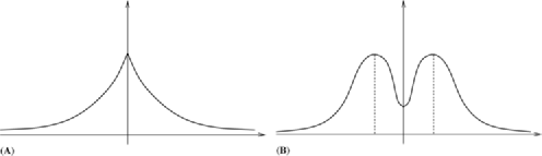
Figure 2: (A) The solution $u_{\nu}(x,t)$, for $0<\nu<1$. (B) The solution $u_{\nu}(x,t)$, for $1<\nu<2$.

Finally it is interesting to analyze the behavior of the solution (for $x$ varying and $t$ fixed), which is substantially different in the two intervals $0<\nu\leq 1$ and $1<\nu\leq 2$ (see Figure 2 above). We rewrite formula (5.3) as follows: for $x>0,$

$$u_{\nu}(x,t)=\frac{1}{\pi\nu}\int_{0}^{+\infty}\frac{g(x,w,t)}{x}e^{-w}\,dw,$$

where $g(x,w,t)=e^{-xA\cos(\nu\pi/2)}\sin(xA\sin(\nu\pi/2))$ and $A=w^{\nu/2}/\lambda t^{\nu/2}$.

The first derivative of $\frac{g(x,w,t)}{x}$ with respect to $x$ is equal to zero if

$$\frac{g_{x}}{g}=\frac{1}{x},$$ (102)

where

$$g_{x} = -A\cos\frac{\nu\pi}{2}e^{-xA\cos(\nu\pi/2)}\sin\biggl{(}xA\sin\frac{\nu\pi}{2}\biggr{)}$$

$${}+A\sin\frac{\nu\pi}{2}e^{-xA\cos(\nu\pi/2)}\cos\biggl{(}xA\sin\frac{\nu\pi}{2}\biggr{)}$$

$$= Ae^{-xA\cos(\nu\pi/2)}\sin\biggl{(}\frac{\nu\pi}{2}-xA\sin\frac{\nu\pi}{2}\biggr{)}.$$

The solution to (102) is

$$\lg g=\lg x+const$$

or, otherwise,

$$g=xconst.$$

By choosing $const=1$, we obtain that $u_{\nu}(x,t)$ attains its maximum on the positive half-line if

$$xe^{xA\cos(\nu\pi/2)}=\sin\biggl{(}xA\sin\frac{\nu\pi}{2}\biggr{)}.$$ (103)

For $1<\nu\leq 2$ there exists only one value of $x$ which verifies the condition (103) and this is in accordance with the behavior of the solutions $u_{\nu}$ presented in Fujita (1990), where the relationship with stable laws is exploited.

On the other hand, for $0<\nu\leq 1,$ no positive value satisfies (103) and therefore the maximum is in the origin. The previous results are confirmed by the following theorems.

We now present the general results concerning the relationship between the solution $u_{\nu}(x,t)$ and the stable densities. We need to analyze the two intervals $0<\nu\leq 1$ and $1<\nu\leq 2$ separately.

Theorem 12.

For $0<\nu\leq 1$, the solution to

$$\cases{\displaystyle\frac{\partial^{\nu}u}{\partial t^{\nu}}=\lambda^{2}\frac{\partial^{2}u}{\partial x^{2}},\cr u(x,0)=\delta(x),}\qquad x\in\mathbb{R},t>0,$$ (104)

can be represented as

$$u_{\nu}(x,t) = \frac{1}{\nu}\frac{\lambda^{2/\nu}t}{|x|^{2/\nu+1}}p_{\nu/2}\biggl{(}\frac{\lambda^{2/\nu}t}{|x|^{2/\nu}};\frac{\nu}{2},1\biggr{)}$$

$$= \frac{1}{\nu|x|^{2/\nu+1}}p_{\nu/2}\biggl{(}\frac{1}{|x|^{2/\nu}};\frac{\nu}{2},\frac{1}{\lambda t^{\nu/2}}\biggr{)}$$

where $p_{\frac{\nu}{2}}(\cdot;\frac{\nu}{2},1)$ is the density of a stable distribution of parameters $\gamma=\frac{\nu}{2}$ and $\eta=1$; see (83).

From (1), by using the reflection formula for the Gamma function we have that

$$u_{\nu}(x,t) = \frac{1}{2\lambda t^{\nu/2}}\sum_{k=0}^{\infty}\biggl{(}-\frac{|x|}{\lambda t^{\nu/2}}\biggr{)}^{k}\frac{1}{k!\Gamma(1-\nu(k+1)/2)}$$

$$= \frac{1}{2\lambda t^{\nu/2}}\sum_{k=0}^{\infty}\biggl{(}-\frac{|x|}{\lambda t^{\nu/2}}\biggr{)}^{k}\frac{1}{k!}\frac{\sin(\pi\nu(k+1)/2)}{\pi}\Gamma\biggl{(}\frac{\nu(k+1)}{2}\biggr{)}.$$

In view of the series representation of stable functions, which for $0<\alpha<1$ reads

$$p_{\alpha}(x;\gamma,1)=\frac{\alpha}{\pi}\sum_{r=0}^{\infty}(-1)^{r}\frac{\Gamma(\alpha(r+1))}{r!}x^{-\alpha(r+1)-1}\sin\biggl{[}\frac{\pi}{2}(\gamma+\alpha)(r+1)\biggr{]}$$

[see Feller (1971), formula (6.10), page 583, with some corrections, Lukacs (1969) and Zolotarev (1986)], we can obtain the first expression in (12). The second expression can be derived by applying the self-similarity property of the stable random variables.

Finally we consider the case $1\leq\nu\leq 2$ and we state the following result:

Theorem 13.

The solution to

$$\cases{\displaystyle\frac{\partial^{\nu}u}{\partial t^{\nu}}=\lambda^{2}\frac{\partial^{2}u}{\partial x^{2}},\cr u(x,0)=\delta(x),\cr u_{t}(x,0)=0,}\qquad x\in\mathbb{R},t>0,$$ (107)

for $1\leq\nu\leq 2$, can be represented as

$$u_{\nu}(x,t) = \frac{2}{\nu}\frac{1}{2\lambda t^{\nu/2}}p_{2/\nu}\biggl{(}\frac{|x|}{\lambda t^{\nu/2}};\frac{2}{\nu}(\nu-1),1\biggr{)}$$

$$= \frac{1}{\nu}p_{2/\nu}\biggl{(}|x|;\frac{2}{\nu}(\nu-1),\lambda^{2/\nu}t\biggr{)},$$

where $p_{2/\nu}(\cdot;\frac{2}{\nu}(\nu-1),1)$ is the density of a stable distribution of parameters $\gamma=\frac{2}{\nu}(\nu-1)$ and $\eta=1$.

By following the same steps as in the previous theorem we can recognize in (5), up to the normalizing constant, the series representation of the stable law $p_{2/\nu}$ of order $\alpha=2/\nu$ [see (84)], so that we get (13).

Remark 5.5.

In view of Theorems 3 and 13 and by considering the property of self-similarity of the stable laws, we can write that

$$u_{\nu}(x,t) = \frac{1}{\nu}\int_{0}^{\infty}\frac{e^{-x^{2}/(4w\lambda)}}{\sqrt{4\pi w\lambda}}\frac{1}{\lambda t^{\nu}}p_{1/\nu}\biggl{(}\frac{|w|}{\lambda t^{\nu}},\frac{1}{\nu}(2\nu-1),1\biggr{)}\,dw$$

$$= \frac{1}{\nu}\int_{0}^{\infty}\frac{e^{-x^{2}/(4w\lambda)}}{\sqrt{4\pi w\lambda}}p_{1/\nu}\biggl{(}|w|,\frac{1}{\nu}(2\nu-1),\lambda^{1/\nu}t\biggr{)}\,dw.$$

Formula (5.5) shows that the solution $u_{\nu},$ for $\frac{1}{2}<\nu\leq 1,$ can be interpreted as the distribution of the process $B(|\mathcal{S}_{\nu}(t)|),$ $t>0$, where $\mathcal{S}_{\nu}$ is the stable process with density $\frac{1}{\nu}p_{1/\nu}(|\cdot|,\frac{1}{\nu}(2\nu-1),\lambda^{1/\nu}t)$.

Moreover, as a consequence of Theorems 2.1 and 5.5, the solution of our problem (1)–(2), for $\frac{1}{2}<\nu\leq 1$, can be written in an alternative to the form (23) also as a stable law evaluated at a Brownian time:

$$u_{\nu}(x,t)=\frac{1}{\nu}\int_{0}^{\infty}\frac{e^{-s^{2}/(4t)}}{\sqrt{\pi t}}\frac{1}{2\lambda s^{\nu}}p_{1/\nu}\biggl{(}\frac{|x|}{\lambda s^{\nu}},\frac{1}{\nu}(2\nu-1),1\biggr{)}\,ds.$$

Remark 5.6.

We check that, for $\nu=1$, both expressions (12) and (13) yield the Gaussian density

$$u_{1}(x,t)=\frac{1}{2\lambda\sqrt{\pi t}}e^{-x^{2}/(4\lambda^{2}t)}.$$ (110)

We start by considering the last expression in (12)

$$u_{1}(x,t)=\frac{1}{|x|^{3}}p_{1/2}\biggl{(}\frac{1}{|x|^{2}};\frac{1}{2},\frac{1}{\lambda t^{1/2}}\biggr{)},$$ (111)

where [from (83)], for $y>0,$

$$p_{1/2}\biggl{(}y;\frac{1}{2},\frac{1}{\lambda t^{1/2}}\biggr{)} = \frac{1}{2\pi}\int_{-\infty}^{+\infty}e^{-i\beta y}\exp\biggl{\{}-\frac{|\beta|^{1/2}}{\lambda t^{1/2}}e^{-i\pi/4\beta/|\beta|}\biggr{\}}\,d\beta$$

$$= \frac{1}{\sqrt{2}\lambda t^{1/2}}\frac{e^{-1/(2y(\sqrt{2}\lambda t^{1/2})^{2})}}{\sqrt{2\pi y^{3}}}.$$

By taking in (5.6) $y=\frac{1}{|x|^{2}}$ we get from (111) the Gaussian density (110). Formula (13) immediately supplies (110) for $\nu=1.$

References

Allouba (2002){barticle}[vtex]
\bauthor\bsnmAllouba, \bfnmHassan\binitsH.
(\byear2002).
\btitleBrownian-time processes: The PDE connection. II. And the
corresponding Feynman–Kac formula.
\bjournalTrans. Amer. Math. Soc.
\bvolume354
\bpages4627–4637 (electronic).
\bmrnumberMR1926892
\endbibitem
Allouba and Zheng (2001){barticle}[msn]
\bauthor\bsnmAllouba, \bfnmHassan\binitsH. and \bauthor\bsnmZheng, \bfnmWeian\binitsW.
(\byear2001).
\btitleBrownian-time processes: The PDE connection and the half-derivative
generator.
\bjournalAnn. Probab.
\bvolume29
\bpages1780–1795.
\bmrnumberMR1880242
\endbibitem
Angulo et al. (2005){barticle}[msn]
\bauthor\bsnmAngulo, \bfnmJ. M.\binitsJ. M.,
\bauthor\bsnmAnh, \bfnmV. V.\binitsV. V.,
\bauthor\bsnmMcVinish, \bfnmR.\binitsR. and \bauthor\bsnmRuiz-Medina, \bfnmM. D.\binitsM. D.
(\byear2005).
\btitleFractional kinetic equations driven by Gaussian or infinitely
divisible noise.
\bjournalAdv. in Appl. Probab.
\bvolume37
\bpages366–392.
\bmrnumberMR2144558
\endbibitem
Angulo et al. (2000){barticle}[msn]
\bauthor\bsnmAngulo, \bfnmJ. M.\binitsJ. M.,
\bauthor\bsnmRuiz-Medina, \bfnmM. D.\binitsM. D.,
\bauthor\bsnmAnh, \bfnmV. V.\binitsV. V. and \bauthor\bsnmGrecksch, \bfnmW.\binitsW.
(\byear2000).
\btitleFractional diffusion and fractional heat equation.
\bjournalAdv. in Appl. Probab.
\bvolume32
\bpages1077–1099.
\bmrnumberMR1808915
\endbibitem
Baeumer, Meerschaert and Nane (2007){bmisc}[vtex]
\bauthor\bsnmBaeumer, \bfnmB.\binitsB.,
\bauthor\bsnmMeerschaert, \bfnmM. M.\binitsM. M.
and \bauthor\bsnmNane, \bfnmE.\binitsE.
(\byear2007).
Brownian subordinators and fractional Cauchy problems. Available at arXiv: 0705.0168v2 [math
PR].
\endbibitem
Beghin and Orsingher (2003){barticle}[msn]
\bauthor\bsnmBeghin, \bfnmLuisa\binitsL. and \bauthor\bsnmOrsingher, \bfnmEnzo\binitsE.
(\byear2003).
\btitleThe telegraph process stopped at stable-distributed times and its
connection with the fractional telegraph equation.
\bjournalFract. Calc. Appl. Anal.
\bvolume6
\bpages187–204.
\bmrnumberMR2035414
\endbibitem
Beghin and Orsingher (2005){barticle}[msn]
\bauthor\bsnmBeghin, \bfnmL.\binitsL. and \bauthor\bsnmOrsingher, \bfnmE.\binitsE.
(\byear2005).
\btitleThe distribution of the local time for “pseudoprocesses” and its
connection with fractional diffusion equations.
\bjournalStochastic Process. Appl.
\bvolume115
\bpages1017–1040.
\bmrnumberMR2138812
\endbibitem
Benachour, Roynette and Vallois (1999){bincollection}[msn]
\bauthor\bsnmBenachour, \bfnmS.\binitsS.,
\bauthor\bsnmRoynette, \bfnmB.\binitsB. and \bauthor\bsnmVallois, \bfnmP.\binitsP.
(\byear1999).
\btitleExplicit solutions of some fourth order partial differential equations
via iterated Brownian motion.
In \bbooktitleSeminar on Stochastic Analysis, Random Fields and
Applications (Ascona, 1996).
\bseriesProgr. Probab.
\bvolume45
\bpages39–61.
\bpublisherBirkhäuser, \baddressBasel.
\bmrnumberMR1712233
\endbibitem
Buckwar and Luchko (1998){barticle}[msn]
\bauthor\bsnmBuckwar, \bfnmEvelyn\binitsE. and \bauthor\bsnmLuchko, \bfnmYuri\binitsY.
(\byear1998).
\btitleInvariance of a partial differential equation of fractional order under
the Lie group of scaling transformations.
\bjournalJ. Math. Anal. Appl.
\bvolume227
\bpages81–97.
\bmrnumberMR1652906
\endbibitem
Burdzy and San Martín (1995){barticle}[msn]
\bauthor\bsnmBurdzy, \bfnmKrzysztof\binitsK. and \bauthor\bsnmSan Martín, \bfnmJaime\binitsJ.
(\byear1995).
\btitleIterated law of iterated logarithm.
\bjournalAnn. Probab.
\bvolume23
\bpages1627–1643.
\bmrnumberMR1379161
\endbibitem
DeBlassie (2004){barticle}[msn]
\bauthor\bsnmDeBlassie, \bfnmR. Dante\binitsR. D.
(\byear2004).
\btitleIterated Brownian motion in an open set.
\bjournalAnn. Appl. Probab.
\bvolume14
\bpages1529–1558.
\bmrnumberMR2071433
\endbibitem
Engler (1997){barticle}[msn]
\bauthor\bsnmEngler, \bfnmHans\binitsH.
(\byear1997).
\btitleSimilarity solutions for a class of hyperbolic integrodifferential
equations.
\bjournalDifferential Integral Equations
\bvolume10
\bpages815–840.
\bmrnumberMR1741754
\endbibitem
Feller (1971){bbook}[vtex]
\bauthor\bsnmFeller, \bfnmWilliam\binitsW.
(\byear1971).
\btitleAn Introduction to Probability Theory and Its Applications
\bvolumeII,
\bedition2nd ed.
\bpublisherWiley, \baddressNew York.
\bmrnumberMR0270403
\endbibitem
Fujita (1990){barticle}[vtex]
\bauthor\bsnmFujita, \bfnmYasuhiro\binitsY.
(\byear1990).
\btitleIntegrodifferential equation which interpolates the heat equation and
the wave equation. II.
\bjournalOsaka J. Math.
\bvolume27
\bpages797–804.
\bmrnumberMR1088183
\endbibitem
Funaki (1979){barticle}[msn]
\bauthor\bsnmFunaki, \bfnmTadahisa\binitsT.
(\byear1979).
\btitleProbabilistic construction of the solution of some higher order
parabolic differential equation.
\bjournalProc. Japan Acad. Ser. A Math. Sci.
\bvolume55
\bpages176–179.
\bmrnumberMR533542
\endbibitem
Gorenflo and Mainardi (1997){bincollection}[msn]
\bauthor\bsnmGorenflo, \bfnmR.\binitsR. and \bauthor\bsnmMainardi, \bfnmF.\binitsF.
(\byear1997).
\btitleFractional calculus: Integral and differential equations of fractional
order.
In \bbooktitleFractals and Fractional Calculus in Continuum Mechanics
(Udine, 1996).
\bseriesCISM Courses and Lectures
\bvolume378
\bpages223–276.
\bpublisherSpringer, \baddressVienna.
\bmrnumberMR1611585
\endbibitem
Gorenflo, Mainardi and Srivastava (1998){binproceedings}[msn]
\bauthor\bsnmGorenflo, \bfnmRudolf\binitsR.,
\bauthor\bsnmMainardi, \bfnmFrancesco\binitsF. and \bauthor\bsnmSrivastava, \bfnmHari M.\binitsH. M.
(\byear1998).
\btitleSpecial functions in fractional relaxation-oscillation and fractional
diffusion-wave phenomena.
In \bbooktitleProceedings of the Eighth International Colloquium on
Differential Equations (Plovdiv, 1997)
\bpages195–202.
\bpublisherVSP, \baddressUtrecht.
\bmrnumberMR1644941
\endbibitem