Periodic orbits, basins of attraction and chaotic beats in two coupled Kerr oscillators.

Abstract

Kerr oscillators are model systems which have practical applications in nonlinear optics. Optical Kerr effect i.e. interaction of optical waves with nonlinear medium with polarizability $\chi^{(3)}$ is the basic phenomenon needed to explain for example the process of light transmission in fibers and optical couplers. In this paper we analyze the two Kerr oscillators coupler and we show that there is a possibility to control the dynamics of this system, especially by switching its dynamics from periodic to chaotic motion and vice versa. Moreover the switching between two different stable periodic states is investigated. The stability of the system is described by the so-called maps of Lyapunov exponents in parametric spaces. Comparison of basins of attractions between two Kerr couplers and a single Kerr system is also presented.

Keywords: Kerr effect, Kerr couplers, Lyapunov exponents, basins of attractions, control of system dynamics, chaotic beats.

1 Introduction

One of the best known and most intensively studied optical models is an oscillator with Kerr nonlinearity. Different kinds of anharmonic Kerr oscillators have also been used to study classical and quantum chaos  [1]- [5]. Mutually coupled Kerr oscillators can be successfully used for a study of couplers, the systems consisting of a pair of coupled Kerr fibres. The first two-mode Kerr coupler has been proposed by Jensen  [6] and investigated in depth in  [6, 7]. Kerr couplers affected by quantization can exhibit various quantum properties such as squeezing of vacuum fluctuations, sub-Poissonian statistics, collapses and revivals  [8, 9].

In the last two decades since the publication of the paper by Pecora and Carroll  [10] the phenomenon of synchronization in systems of the coupled oscillators has become a subject of comprehensive investigation. The problem of synchronization of two linearly coupled Kerr oscillators has been studied in  [11] and the possibility of synchronization of chaotic motion was proved numerically. Moreover the case of synchronization of two kinds of Kerr couplers having a structure of low-dimensional chains (ring and open) has been analysed  [12].

This paper is an attempt at using the modern tools of nonlinear science for numerical investigation of dynamics of a system made of two coupled Kerr oscillators.

In Sec. 2 the basic equation of motion for the single Kerr oscillator is introduced. Simple periodic solutions of equations of motions have been found and the dynamics of the system as well as basins of attraction for such solutions are investigated. Moreover, we calculate the Lyapunov maps for the single Kerr oscillator with external periodic as well as modulated fields. The second case of the external field is used to generate the so-called chaotic beats. In Sec. 3 our single Kerr system analysis is extended over the case of two coupled Kerr sub-systems with nonlinear coupling. We find the analytic periodic solutions of such a system. Lyapunov maps and the basins of attraction for this system are helpful tools in analysis of properties of these system. We find that it is possible to change the periodic states of one sub-system by changing the initial conditions of the other sub-system (switching the periodic dynamics). Moreover, it is proved that coupled Kerr sub-systems are able to generate of chaotic beats.

2 The single Kerr oscillator

2.1 Equations of motion

We study the dynamical system described by the following hamiltonian:

$$H=H_{0}+H_{1}\,,$$ (1)

where:

$$H_{0} = \omega a^{*}a+\frac{1}{2}\epsilon a^{*2}a^{2}\,,$$ (2)

$$H_{1} = iF\left(a^{*}e^{-i\Omega_{p}t}-ae^{i\Omega_{p}t}\right)\,.$$ (3)

The hamiltonian $H_{0}$ represents the so called Kerr oscillator (if $\epsilon=0$, then $H_{0}$ refers to the harmonic oscillator), whereas the hamiltonian $H_{1}$ describes the interaction of the Kerr oscillator with the periodic external field. The quantities $a$ and $a^{*}$ are complex dynamical variables describing the amplitudes, $\omega$ denotes the frequency of the free vibrations of the harmonic oscillator - basic frequency, $\epsilon$ is the parameter describing the Kerr nonlinearity in the system (this is the nonlinearity of the third order) and $F$ is the external field amplitude at the frequency $\Omega_{p}$.

The equation of motion for variable $a$ has the form:

$$\frac{da}{dt}=-i\omega a-i\epsilon a^{*}a^{2}+Fe^{-i\Omega_{p}t}-\gamma a\,.$$ (4)

The term $-\gamma a$ - added on phenomenological grounds - describes the mechanism of loss with the damping constant $\gamma$. All the parameters, that is $\omega$, $\epsilon$, $F$, $\Omega_{p}$ and $\gamma$ are taken to be real. The equation of motion for $a^{*}$ is simply a complex conjugation of Eq.(4).

In the autonomous and conservative case, that is when $\gamma=F=0$, the solution of equation (4) has a well-known form:

$$a(t)=a_{0}e^{-i(\omega+\epsilon a_{0}^{*}a_{0})t}\,,$$ (5)

where $a(t)\mid_{t=0}=a_{0}$ is the initial condition.

In the nonautonomous case of Eq.(4) we can find the periodic solution:

$$a(t)=xe^{-i(\omega+\epsilon x^{*}x)t}\,,$$ (6)

that is in the form of the solution of the autonomous one. Function (6) satisfies the equation of motion (4) provided that $x=F/\gamma$. As a result the periodic solution of equation (4) has the form:

$$a(t)=\frac{F}{\gamma}e^{-i\left(\omega+\epsilon\frac{F^{2}}{\gamma^{2}}\right)t}\,.$$ (7)

Formally, the function in the form of (7) is the solution of the differential equation (4) only if two condition are fulfilled: (A) $\Omega_{p}=\omega+\epsilon\frac{F^{2}}{\gamma^{2}}$, and (B) the initial condition has the form $a(0)\equiv a_{0}=F/\gamma$. In other words, the periodic solution (7) is correct only for special choice of the set of parameters $\omega,\Omega_{p},F,\gamma$. Finally, it is worth noting that in the nonautonomous case the period of solution (7) depends on the initial condition, as well as in the autonomous case. In the phase plane $(\mathit{Re}\,a,\,\mathit{Im}\,a)$ the periodic solution (7) satisfies the phase equation (circle):

$$(\mathit{Re}\,a)^{2}+(\mathit{Im}\,a)^{2}=F^{2}/\gamma^{2}\,.$$ (8)

for any values of frequency $\omega$.

It should be emphasized that the method presented here is usefull to find only the one periodic solution for a given set of the system parameters. Generally, the Eq. (4) have up to three (not only periodic) solutions.

2.2 The dynamics of the system in the phase space

As a numerical example let us consider the dynamics of a system described by equation (4), if $\omega=1$, $\gamma=0.5$, $\epsilon=0.01$, $F=5$ and $\Omega_{p}=2$. Then, in compliance with (7), the periodic solution of equation (4) has the form:

$$a(t)=10e^{-2it}\,,$$ (9)

and in the phase space it satisfies the following equation:

$$(\mathit{Re}\,a)^{2}+(\mathit{Im}\,a)^{2}=100\,.$$ (10)

As a result, for the initial condition $a_{0}=10$ the phase point draws simply a circle described by equation (10). But if the system (4) starts from another initial conditions, we observe the following interesting behaviour: after some time the phase point tends to one of the two orbits: $(\mathit{Re}\,a)^{2}+(\mathit{Im}\,a)^{2}=100$ or $(\mathit{Re}\,a)^{2}+(\mathit{Im}\,a)^{2}=50$. Two examples of such behaviour of the phase point are illustrated in Fig. 1.

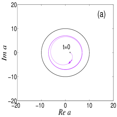
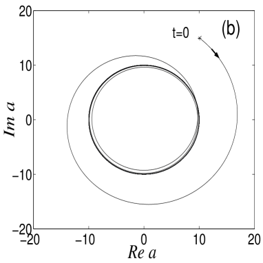
Figure 1: The phase trajectories of the system (4) for $\omega=1$, $\gamma=0.5$, $\epsilon=0.01$, $F=5$ and $\Omega_{p}=2$ and for the initial conditions: (a) $\mathit{Re}\,a=2$, $\mathit{Im}\,a=0$; (b) $\mathit{Re}\,a=10$, $\mathit{Im}\,a=15$.

In Fig. 1(a) the phase point (marked in pink) starts from the initial condition $\mathit{Re}\,a=2$, $\mathit{Im}\,a=0$ and after the time $t=50$ goes into the orbit of the radius $r=\sqrt{50}$. However in Fig. 1(b) we can see how the phase point starting from the initial condition $\mathit{Re}\,a=10$, $\mathit{Im}\,a=15$ goes into the orbit of the radius $r=10$, described by equation (10). It should be emphasized that the orbit $r=\sqrt{50}$ is also periodic but it does not fulfill conditions (A) and (B).

Both orbits: $(\mathit{Re}\,a)^{2}+(\mathit{Im}\,a)^{2}=100$ and $(\mathit{Re}\,a)^{2}+(\mathit{Im}\,a)^{2}=50$ are attractors of the system (4). It means that for the parameters: $\omega=1$, $\gamma=0.5$, $\epsilon=0.01$, $F=5$ and $\Omega_{p}=2$ the system (4) tends to one of the two steady states (periodic), represented by these two orbits.

It is easy to show that the orbit described by equation $(\mathit{Re}\,a)^{2}+(\mathit{Im}\,a)^{2}=50$ is identical with that generated by equation (4) if $\omega=1$, $\gamma=0.5$, $\epsilon=0.01$, $F=5$ and $\Omega_{p}=1$ and for the initial condition: $\mathit{Re}\,a=5$, $\mathit{Im}\,a=5$. This solution has the form: $a(t)=(5+5i)e^{-2it}$.

2.3 Basin of attraction

To illustrate the full influence of the initial conditions on the evolution of the system we used the so called basins of attraction. Basin of attraction is the set of initial conditions which lead to the system’s attractor. The basins of attraction of the system (4) for $\omega=1$, $\gamma=0.5$, $\epsilon=0.01$, $F=5$ and $\Omega_{p}=2$ are presented in Fig.2. There are two attractors of the system (limit cycles $r=10$ and $r\prime=\sqrt{50}$) and their basins of attraction are marked by different colours, the yellow area marks the basin of attraction of the attractor $(\mathit{Re}\,a_{1})^{2}+(\mathit{Im}\,a_{1})^{2}=100$, whereas the blue one refers to the basin of attraction of the attractor $(\mathit{Re}\,a_{1})^{2}+(\mathit{Im}\,a_{1})^{2}=50$. Both basins have interesting geometries. The basin corresponding to the circle of the radius $r\prime=\sqrt{50}$ has a spiral-like form with the slip and width decreasing when moving away from the centre. The remaining area (blue colour) refers to the basin of attraction of the second attractor (the circle of the radius $r=10$). Both attractors have a special property. They are localised in such a way, that each attractor is located partly in its own basin of attraction and partly in the basin of attraction of the other attractor. As a result - if the phase point starts from the part of the attractor situated in the basin of attraction of the other one, it escapes to the other attractor. However, if it starts from the part of the attractor situated in its own basin of attraction, it does not change the attractor. In analogy to semistable orbits these attractors can be called the semistable attractors. So, the system with Kerr nonlinearity is tuneable: an adequate choice of the initial condition can result in the transition of the phase point from the one attractor to the other. This property seems to be useful in applications in optical switches.

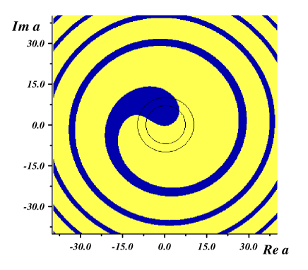
Figure 2: Basins of attraction for two attractors - limit cycles for $r=10$ and $r\prime=\sqrt{50}$. The parameters of the system (7) are: $\omega=1$, $\gamma=0.5$, $\epsilon=0.01$, $F=5$ and $\Omega_{p}=2$.

2.4 Parameters detuning

One of the important properties of dynamical systems is their sensitivity to the change in the system’s parameters. A small change in a parameter can lead to radical changes in the dynamics of the system. This feature is frequently used to control the dynamical systems. Globally, the behaviour of the system can be shown on the so-called Lyapunov map in a parametric space. We used here the well known procedure  [13] for numerical calculation of Lyapunov exponents (Lyapunov spectrum $\lambda_{i},i=1,2$). In Fig.3 we show the map of maximal Lyapunow exponent $\lambda_{1}$ for the parameters of the system $\omega=1$, $\epsilon=0.01$ and for the pump field amplitude $F=5$. The map is presented in the parameters space ($\Omega_{p}$, $\gamma$). The highest values of $\lambda_{1}$ corresponding to chaotic oscillations are marked by red and blue colours. The chaotic motion exists only for weak damping. For higher damping constants we find only single islands of chaotic motion in the pump field parametric space ($\Omega_{p}$, $F$) (see Fig.4).

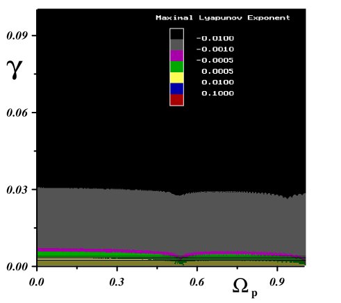
Figure 3: Lyapunov map - the values of the maximal Lyapunow exponent $\lambda_{1}$ for the parameters of the system (11): $\omega=1$, $\epsilon=0.01$ and for the pump field amplitude $F=5$. The initial condition is: $\mathit{Re}\,a=10$, $\mathit{Im}\,a=0$. In the parameter space ($\Omega_{p}$, $\gamma$) the colours correspond to appropriate values of $\lambda_{1}$.

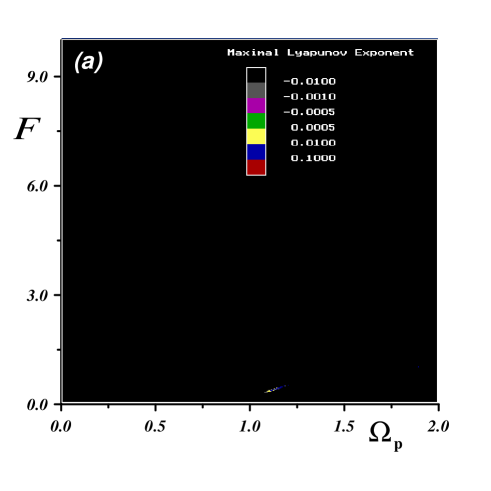
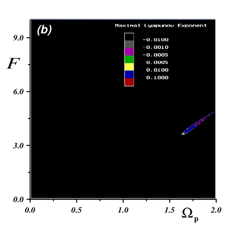
Figure 4: Lyapunov maps - the values of the maximal Lyapunow exponent $\lambda_{1}$ for the parameters of the system (11): $\omega=1$, $\epsilon=0.01$ and for the initial condition: $\mathit{Re}\,a=10$, $\mathit{Im}\,a=0$. The parameter spaces ($\Omega_{p}$, $F$) are presented for (a) $\gamma=0.1$ and (b) $\gamma=0.5$. For higher values of $\gamma$ only the periodic behaviour of the system is observed.

To control our system of Kerr oscillators we first change the value of one of the parameters ($\gamma$, $F$ or $\Omega_{p}$) of the system (4) at time $t_{1}$. In such a way, the phase point being in one of the two orbits (attractors) shown in Fig.2 escapes from the attractor to the transient state and sometimes to the new periodic state. Then after returning at time $t_{2}>t_{1}$ to the initial values of this parameter, the additional periodic state disappears and the phase point trajectory tends to one of the two attractors of the system, depending on which basin of attraction was the phase point at time $t_{2}$ . So, through the appropriate choices of times $t_{1}$ end $t_{2}$ as well as the values of the parameters of the system we can control its evolution. In particular, we can switch the system between two stable periodic states. Such situations are illustrated in Fig. 5(a)–(c).

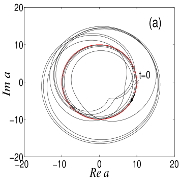
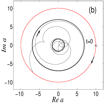
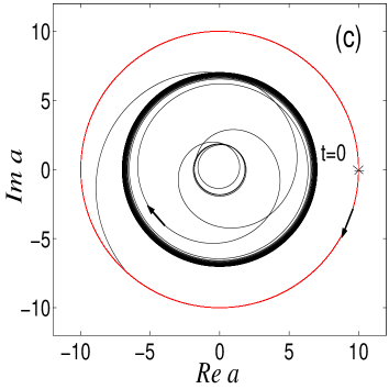
Figure 5: The phase trajectories of the system (5) for the initial conditions: $\mathit{Re}\,a=10$, $\mathit{Im}\,a=0$ and for the following values of the system’s parameters: (a) $\omega=1$, $\epsilon=0.01$, $F=5$, $\Omega_{p}=2$ and $\gamma=0.5$ for $0<t<20$, $\gamma=0.02$ for $20<t<40$ and $\gamma=0.5$ for $40<t<60$; (b) $\omega=1$, $\gamma=0.5$, $\epsilon=0.01$, $F=5$ and $\Omega_{p}=2$ for $0<t<20$, $\Omega_{p}=4$ for $20<t<40$ and $\Omega_{p}=2$ for $40<t<100$; (c) $\omega=1$, $\gamma=0.5$, $\epsilon=0.01$, $\Omega_{p}=2$ and $F=5$ for $0<t<20$, $F=2$ for $20<t<40$ and $F=5$ for $40<t<250$.

In Fig.5(a) the phase point starting from the orbit of the radius $r=10$ (marked in red) after detuning the value of the damping constant $\gamma$ in time $t_{1}=20$ from $\gamma=0.5$ to $\gamma=0.02$ escapes through a transient state to the new periodic state $r=11,91$. After coming back with $\gamma$ to the initial value $\gamma=0.5$ it goes into the initial orbit (of the radius $r=10$). In Fig. 5(b) the phase point starts also from the point lying on the orbit of the radius $r=10$ and after detuning the parameter $\Omega_{p}$ from $\Omega_{p}=2$ to $\Omega_{p}=4$ at time $t_{1}=20$ it escapes through a transient state to the new periodic state $r=1,84$. Then after coming back with the parameter $\Omega_{p}$ at time $t_{2}=40$ to the initial value $\Omega_{p}=2$ it goes into the orbit of the radius $r\prime=\sqrt{50}$ - the case of switching between the periodic orbits. Moreover, Fig.5(c) shows the phase point starting from the site lying on the orbit of the radius $r=10$ after detuning the value of the parameter $F$ from $F=5$ to $F=2$ at time $t_{1}=20$ also moves to another periodic orbit $r=1,84$, and then after returning at time $t_{2}=40$ to the initial value of parameter $F$ ($F=5$) it goes into the orbit of the radius $r\prime=\sqrt{50}$. Generally, it is very interesting that if we change the parameters of the system, some extra periodic orbits appear.

2.5 Generation of chaotic beats

Since the publication of  [14], the new type of signals called ”chaotic beats” has been investigated  [15] and experimentally generated  [16, 19]. There are two basic kinds of chaotic beats: (1) the signals with chaotic envelopes and a stable fundamental frequency, and (2) the signals with almost regular collapses and revivals with small chaotic perturbations. Generally, when the system is subjected to an external field, we can generate the chaotic beats in two ways by modulation of the amplitude or frequency of the external field.

The more effective method of generation of chaotic beats in system (4) seems to be the frequency modulation, according to the formula:

$\Omega_{p}\rightarrow\Omega_{p}(1+\Delta\Omega_{p}\sin(\mu t))$,

where $\mu$ is the frequency of modulation parameter, and $\Delta\Omega_{p}$ is the amplitude of this modulation. Then the equation of motion for variable $a$ takes the form:

$$\frac{da}{dt}=-i\omega a-i\epsilon a^{*}a^{2}-\gamma a+Fe^{-i\Omega_{p}(1+\Delta\Omega_{p}\sin(\mu t))t}\;.$$ (11)

In numerical calculations we put $\Delta\Omega_{p}=0.1$.

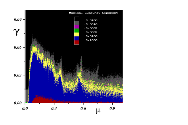
Figure 6: The values of maximal Lyapunov exponent $\lambda_{1}$ for the system (11) as a function of the damping parameter $\gamma$ and the frequency modulation $\mu$, for $\epsilon=0.01$, $F=5$, $\Omega_{p}=2$ and with the initial condition: $\mathit{Re}\,a=10$, $\mathit{Im}\,a=0$.

The global dynamics of system (11) is presented in Fig. 6 as a Lyapunov map in the parametric space of $(\gamma,\mu)$, where the values of the first Lyapunov exponent $\lambda_{1}$ are marked by appropriate colours. The highest values of $\lambda_{1}$ corresponding to chaotic oscillations are marked by red and blue colours. As we can see, they are concentrated in the lower part of the map which corresponds to the low values of the damping parameter $\gamma$ (mainly for $\gamma<0.05$). For higher $\gamma$ the map is dominated by the black and grey colours corresponding to the periodic states. An example of chaotic beats generated in the system (11) through frequency modulation (with $\gamma=0.02$ and $\mu=0.15$) is presented in Fig.7. The spectrum of the Lyapunov exponents $\{0.0519,-0.0813\}$ of that system with the positive value of $\lambda_{1}$ indicates chaotic behaviour.

Similar results were obtained for the resonance case ($\Omega_{p}=\omega$). The values of maximal Lyapunov exponent $\lambda_{1}$ for system (11) as a function of the damping parameter $\gamma$ ($0<\gamma<0.5$) and the frequency modulation $\mu$ ($0<\mu<1$) and for $\Omega_{p}=\omega=1$ are presented in Fig.8.

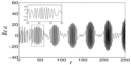
Figure 7: Time dependence of $\mathit{Re}\,a$ of the system (11), for $\gamma=0.02$ and $\mu=0.15$. The other parameters are: $\omega=1$, $F=5$, $\epsilon=0.01$ and $\Omega_{p}=2$. The system starts from the initial condition: $\mathit{Re}\,a=10$, $\mathit{Im}\,a=0$. Chaotic beats.

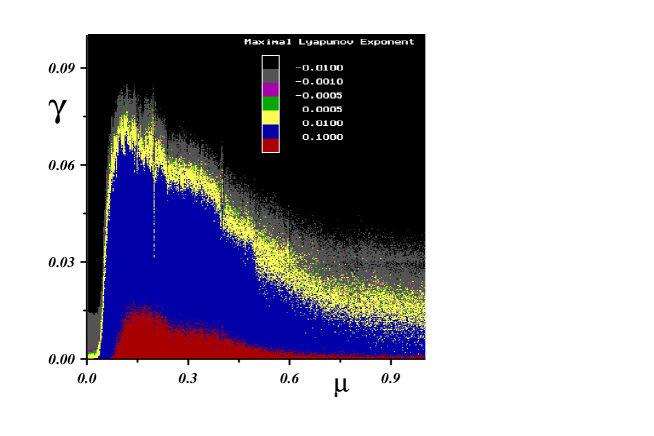
Figure 8: The values of the maximal Lyapunov exponent $\lambda_{1}$ of system (11) as a function of the damping parameter $\gamma$ and the frequency of modulation $\mu$, for $\epsilon=0.01$, $F=5$ and $\Omega_{p}=\omega=1$ (the resonant case) and with the initial conditions: $\mathit{Re}\,a=10$, $\mathit{Im}\,a=0$.

Analogically as for the non-resonance case, the chaotic behaviour is obtained only for the low values of the damping parameter $\gamma$ (mainly for $\gamma<0.05$). In Fig.9 we can see the time dependence of $\mathit{Re}\,a$ of the system (11), for $\gamma=0.01$, $\mu=0.15$ and $\Omega_{p}=\omega=1$.

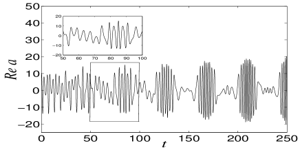
Figure 9: Time dependence of $\mathit{Re}\,a$ of system (11), for $\gamma=0.01$, $\mu=0.15$, $F=5$, $\epsilon=0.01$ and $\Omega_{p}=\omega=1$. The system starts from the initial condition: $\mathit{Re}\,a=10$, $\mathit{Im}\,a=0$. Chaotic beats.

The spectrum of Lyapunov exponents of the beats shown in Fig.9 is $\{0.1085,-0.1230\}$ and contains positive value of $\lambda_{1}$ indicating chaotic behaviour.

3 The two coupled Kerr oscillators

3.1 Equations of motion

It is interesting to know what happens to the dynamics of the single Kerr oscillator after coupling it nonlinearly to another analogous oscillator but of different frequency. Such a system of two nonlinearly coupled Kerr oscillators (nonlinear couplers) is described by the following hamiltonian:

$$H=H_{0}+H_{1}+H_{2}\,,$$ (12)

where:

$$H_{0} = \sum_{j=1}^{2}\omega_{j}a_{j}^{*}a_{j}+\frac{1}{2}\sum_{j=1}^{2}\epsilon_{j}a_{j}^{*2}a_{j}^{2}\,,$$ (13)

$$H_{1} = \epsilon_{12}a_{1}^{*}a_{2}^{*}a_{1}a_{2}\,,$$ (14)

$$H_{2} = i\sum_{j=1}^{2}\left[F_{j}\left(a_{j}^{*}e^{-i\Omega_{jp}t}-a_{j}e^{i\Omega_{jp}t}\right)\right]\,.$$ (15)

The hamiltonian $H_{0}$ represents the two single Kerr oscillators, $H_{1}$ is the hamiltonian of the interaction between them and $H_{2}$ describes the interaction of the two oscillators with the external fields. The values $a_{1}$ and $a_{2}$ are complex dynamical variables, $\omega_{j}$ denote the frequencies of the free vibrations of the two single oscillators; $\epsilon_{1}$ and $\epsilon_{2}$ are Kerr parameters describing nonlinearity in these sub-systems (oscillators) and $\epsilon_{12}$ is the parameter of nonlinear coupling between them.

The equations of motion for variables $a_{1}$ and $a_{2}$ have the form:

$$\frac{da_{1}}{dt} = -i\omega_{1}a_{1}-i\epsilon_{1}a_{1}^{*}a_{1}^{2}-i\epsilon_{12}a_{2}^{*}a_{1}a_{2}+$$

$$+ F_{1}e^{-i\Omega_{1p}t}-\gamma_{1}a_{1}\,,$$

$$\frac{da_{2}}{dt} = -i\omega_{2}a_{2}-i\epsilon_{2}a_{2}^{*}a_{2}^{2}-i\epsilon_{12}a_{1}^{*}a_{1}a_{2}+$$

$$+ F_{2}e^{-i\Omega_{2p}t}-\gamma_{2}a_{2}\,,$$

where the terms $\gamma_{1}a_{1}$ and $\gamma_{2}a_{2}$, describing the dissipation of energy, with damping constants $\gamma_{1}$ and $\gamma_{2}$, are added to the equations of motion on phenomenological grounds. In the autonomous and conservative case, that is when $\gamma_{1}=\gamma_{2}=F_{1}=F_{2}=0$ the solutions of equations (3.1)–(3.1) have the form:

$$a_{1}(t) = a_{10}e^{-i(\omega_{1}+\epsilon_{1}a_{10}^{*}a_{10}+\epsilon_{12}a_{20}^{*}a_{20})t}\,,$$ (18)

$$a_{2}(t) = a_{20}e^{-i(\omega_{2}+\epsilon_{2}a_{20}^{*}a_{20}+\epsilon_{12}a_{10}^{*}a_{10})t}\,,$$ (19)

where $a_{1}(t)\mid_{t=0}\equiv a_{10}$ and $a_{2}(t)\mid_{t=0}\equiv a_{20}$ denote initial conditions.
In the nonautonomous case (3.1)–(3.1) we find periodic solutions in the form of the following functions (in analogy to the case of the single Kerr oscillator):

$$a_{1}(t) = x_{1}e^{-i(\omega_{1}+\epsilon_{1}x_{1}^{*}x_{1}+\epsilon_{12}x_{2}^{*}x_{2})t}\,,$$ (20)

$$a_{2}(t) = x_{2}e^{-i(\omega_{2}+\epsilon_{2}x_{2}^{*}x_{2}+\epsilon_{12}x_{1}^{*}x_{1})t}\,,$$ (21)

that is in the form of the solutions of the autonomous one. Functions (20)–(21) satisfy the equations of motion (3.1)–(3.1) on condition that $x_{j}=F_{j}/\gamma_{j}$, $j=1,2$. As a result these solutions have the form:

$$a_{1}(t) = \frac{F_{1}}{\gamma_{1}}\exp\left[-i\left(\omega_{1}+\epsilon_{1}\frac{F_{1}^{2}}{\gamma_{1}^{2}}+\epsilon_{12}\frac{F_{2}^{2}}{\gamma_{2}^{2}}\right)t\right]\,,$$ (22)

$$a_{2}(t) = \frac{F_{2}}{\gamma_{2}}\exp\left[-i\left(\omega_{2}+\epsilon_{2}\frac{F_{2}^{2}}{\gamma_{2}^{2}}+\epsilon_{12}\frac{F_{1}^{2}}{\gamma_{1}^{2}}\right)t\right]\,.$$ (23)

Then $\Omega_{1p}=\omega_{1}+\epsilon_{1}F_{1}^{2}/\gamma_{1}^{2}+\epsilon_{12}F_{2}^{2}/\gamma_{2}^{2}$ and $\Omega_{2p}=\omega_{2}+\epsilon_{2}F_{2}^{2}/\gamma_{2}^{2}+\epsilon_{12}F_{1}^{2}/\gamma_{1}^{2}$.
In the phase plane $(\mathit{Re}\,a_{1},\,\mathit{Im}\,a_{1},\,\mathit{Re}\,a_{2},\,\mathit{Im}\,a_{2})$ the periodic solutions (22)–(23) satisfy the phase equations (limit cycles - circles):

$$(\mathit{Re}\,a_{j})^{2}+(\mathit{Im}\,a_{j})^{2}=\frac{F_{j}^{2}}{\gamma_{j}^{2}}\,,\,\,\,\,\,\mbox{where $j=1,2$},$$ (24)

for any values of frequencies $\omega_{1}$, $\omega_{2}$.

3.2 The dynamics of the system in the phase space

Coupling the single Kerr oscillator described by equation (4) to the other analogous oscillator but with different own frequency causes distinct changes in its dynamics, as illustrated by the diagrams in the phase space.

Let us consider two nonlinearly coupled Kerr oscillators (sub-systems) described by equations (3.1)–(3.1) if $\omega_{1}=1$, $\omega_{2}=0.5$, $\epsilon_{1}=\epsilon_{2}=0.01$, $F_{1}=F_{2}=5$, $\gamma_{1}=\gamma_{2}=0.5$, $\Omega_{1p}=3.0$, $\Omega_{2p}=2.5$ and $\epsilon_{12}=0.01$. Then, in compliance with (22)–(23), the periodic solutions of equations (3.1)–(3.1) have the form:

$$a_{1}(t) = 10e^{-3.0it}\,,$$ (25)

$$a_{2}(t) = 10e^{-2.5it}\,,$$ (26)

and in the phase space they satisfy the following equations:

$$(\mathit{Re}\,a_{1})^{2}+(\mathit{Im}\,a_{1})^{2} = 100\,,$$ (27)

$$(\mathit{Re}\,a_{2})^{2}+(\mathit{Im}\,a_{2})^{2} = 100\,.$$ (28)

As a result, for the initial conditions $a_{10}=10$ and $a_{20}=10$ the phase points of both subsystems draw the same circle of the radius $r=10$ described by equations (27)–(28), with frequencies $\Omega_{1p}=3.0$ and $\Omega_{2p}=2.5$, respectively. But if the phase point representing the first subsystem (at frequency $\omega_{1}=1$) starts from another initial condition instead of $a_{10}=10$, and $a_{20}$ is fixed ($a_{20}=10$), the following behaviour is observed: the phase point representing the first sub-system after some time tends to one of the two orbits being attractors of subsystem (3.1): $(\mathit{Re}\,a_{1})^{2}+(\mathit{Im}\,a_{1})^{2}=100$ or $(\mathit{Re}\,a_{1})^{2}+(\mathit{Im}\,a_{1})^{2}=6.6987$. The second orbit belongs to the periodic solution: $a_{1}(t)=(10/(1-i(2-\sqrt{3}))exp(-3.0it)$ and $a_{2}(t)=(10/(1-i(2-\sqrt{3}))exp(-2.5it)$. This situation is illustrated in Fig. 10.

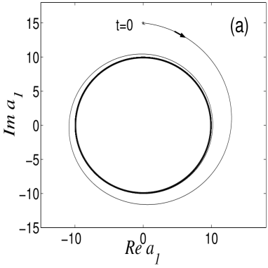
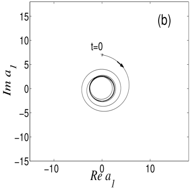
Figure 10: The phase trajectories of sub-system (3.1) if $\omega_{1}=1$, $\omega_{2}=0.5$, $\epsilon_{1}=\epsilon_{2}=0.01$, $F_{1}=F_{2}=5$, $\gamma_{1}=\gamma_{2}=0.5$, $\Omega_{1p}=3.0$, $\Omega_{2p}=2.5$, $\epsilon_{12}=0.01$ and for the initial conditions: (a) $\mathit{Re}\,a_{10}=0$, $\mathit{Im}\,a_{10}=15$, $\mathit{Re}\,a_{20}=10$, $\mathit{Im}\,a_{20}=0$; (b) $\mathit{Re}\,a_{10}=0$, $\mathit{Im}\,a_{10}=7$, $\mathit{Re}\,a_{20}=10$, $\mathit{Im}\,a_{20}=0$.

In Fig. 10(a) the phase point representing the first sub-system starts from the initial condition $\mathit{Re}\,a_{10}=0$, $\mathit{Im}\,a_{10}=15$ (the initial condition for the second subsystem (3.1) is fixed: $\mathit{Re}\,a_{20}=10$, $\mathit{Im}\,a_{20}=0$) and after the time $t=50$ it goes into the attractor of the radius $r=10$, described by equation (27). However, Fig.10(b) shows the phase point starting from the initial condition $\mathit{Re}\,a_{10}=0$, $\mathit{Im}\,a_{10}=7$ and going into the orbit of the radius $r^{\prime}=\sqrt{6.6987}$.

The third solution of (16) and (17) is completely unstable and has the form:
$a_{1}(t)=(10/(1-i(2+\sqrt{3}))exp(-3.0it)$
and $a_{2}(t)=(10/(1-i(2+\sqrt{3}))exp(-2.5it)$.

3.3 Basins of attraction

Fig.11 shows two attractors and their basins of attraction of sub-system (3.1) marked by appropriate colours; the initial condition of sub-system (3.1) is fixed ($a_{20}=10$). The yellow area marks the basin of attraction of the attractor of the radius $r=10$, whereas the blue one corresponds to the basin of attraction of the attractor of the radius $r^{\prime}=\sqrt{6.6987}$. The basin marked in yellow has a special geometry: it consists of two separate areas, one of which has a spiral-like form. Both, the slip of the spiral and its width decrease towards moving away from the centre, similarly, as for the single Kerr oscillator. Contrary to the case of the single Kerr oscillator there is an island in the central part of the basin. The remaining area (blue colour) is the basin of attraction of the other attractor (the circle of the radius $r^{\prime}=\sqrt{6.6987}$).

The attractor of the radius $r^{\prime}=\sqrt{6.6987}$ is stable (it is fully in its own basin of attraction), however the attractor of the radius $r=10$ is semistable (it is partly in its own basin of attraction and partly in the basin of attraction of the other attractor). As a result the transition from the attractor of the radius $r=10$ to the attractor of the radius $r^{\prime}=\sqrt{6.6987}$ is possible, but that in opposite direction is impossible, because the phase point starting from any position on the circle $(\mathit{Re}\,a)^{2}+(\mathit{Im}\,a)^{2}=6.6987$ always returns to it.

The types of attractors change after changing the initial condition of the sub-system (3.1). For example, Fig.12 shows the attractors and their basins of attractions of sub-system (3.1) for $a_{20}=0$. The basin of attraction corresponding to the circle of the radius $r=10$ is marked by yellow; the remaining area (blue colour) refers to the basin of attraction of the circle of $r^{\prime}=\sqrt{6.6987}$. As we can see, in this case the attractor with radii ($r^{\prime}=\sqrt{6.6987}$) is stable, and the other one is completely unstable.

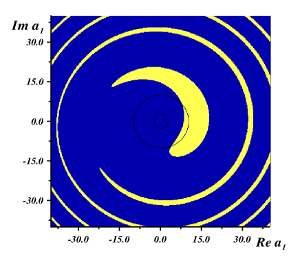
Figure 11: Basins of attraction of two coupled Kerr oscillators. The parameters of the systems are: $\omega_{1}=1$, $\omega_{2}=0.5$, $\epsilon_{1}=\epsilon_{2}=0.01$, $F_{1}=F_{2}=5$, $\gamma_{1}=\gamma_{2}=0.5$, $\Omega_{1p}=3.0$, $\Omega_{2p}=2.5$, $\epsilon_{12}=0.01$, and the initial conditions are: $\mathit{Re}\,a_{10}=0$, $\mathit{Im}\,a_{10}=15$, $\mathit{Re}\,a_{20}=10$, $\mathit{Im}\,a_{20}=0$. Stable ($r^{\prime}=\sqrt{6.6987}$) and semistable ($r=10$) attractors.

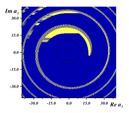
Figure 12: Basins of attraction of two coupled Kerr oscillators. The parameters are the same as in Fig. 11, but $\mathit{Re}\,a_{20}=0$, $\mathit{Im}\,a_{20}=0$. Stable ($r^{\prime}=\sqrt{6.6987}$) and unstable ($r=10$) attractors.

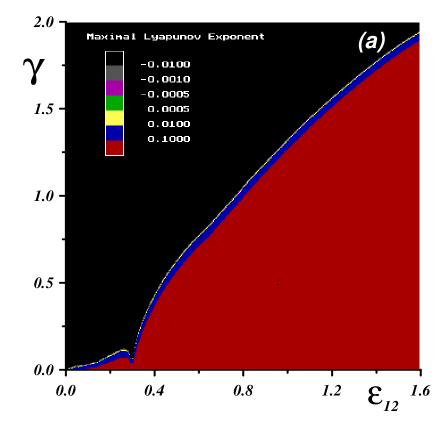
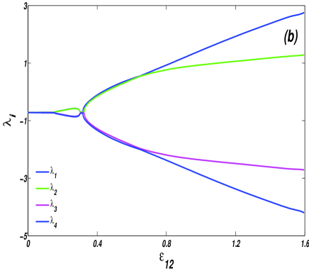
Figure 13: (a) The Lyapunov map of the system (3.1)–(3.1) in the parametric space ($\epsilon_{12},\gamma$) where $\gamma=\gamma_{1}=\gamma_{2}$. (b) The full spectrum of Lyapunov exponents $\{\lambda_{1},\lambda_{2},\lambda_{3},\lambda_{4}\}$ of the system (3.1)–(3.1) as a function of the nonlinear coupling parameter $\epsilon_{12}$ and for $\gamma=\gamma_{1}=\gamma_{2}=0.5$. The rest of parameters for both figures are: $\omega_{1}=1$, $\omega_{2}=0.5$, $\epsilon_{1}=\epsilon_{2}=0.01$, $F_{1}=F_{2}=5$, $\Omega_{1p}=3$ and $\Omega_{2p}=2.5$. The system starts from the initial conditions: $\mathit{Re}\,a_{1}=10$, $\mathit{Im}\,a_{1}=0$, $\mathit{Re}\,a_{2}=10$, $\mathit{Im}\,a_{2}=0$

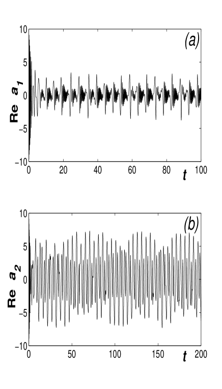
Figure 14: Time dependence of $\mathit{Re}\,a_{1}$ (a) and $\mathit{Re}\,a_{2}$ (b) of the system (3.1)–(3.1). Parameters are the same as in Fig.13(b), and $\epsilon_{12}=0.45$. Chaotic beats.

3.4 Generation of chaotic beats

Globally, the behaviour of system (3.1)–(3.1) is presented in Fig.13(a) showing the Lyapunov map in the parameters space ($\epsilon_{12},\gamma$). We find that strong chaotic behaviour of the system is much common that for the single Kerr system. We also notice that if we increase the dumping in the system we must increase the coupling between subsystems to achieve the chaotic behaviour. The full spectrum of the Lyapunov exponents $\{\lambda_{1},\lambda_{2},\lambda_{3},\lambda_{4}\}$ versus $\epsilon_{12}$ shows the regions of order or chaos in the cross section of the map for the damping parameter $\gamma=\gamma_{1}=\gamma_{2}=0.5$ (Fig.13(b)). If $\lambda_{1}>0$ then the system is chaotic, and if $\lambda_{1}\leq 0$, it behaves periodically. The system with the parameters of Fig. 13 and for the coupling constant $\epsilon_{12}>1.6$ manifests extremely unstable behaviour and its solutions are divergent to infinity. There is also a region of hyperchaotic behaviour of the system in which two highest Lyapunov exponents are positive (for $\epsilon_{12}>0.44$).

Taking from Fig.13(a)-(b) the appropriate values of the damping constant $\gamma_{1}=\gamma_{2}=0.5$ and the nonlinear coupling between the Kerr oscillators $\epsilon_{12}=0.45$ we can generate chaotic beats in the system of two nonlinearly coupled Kerr oscillators (3.1)–(3.1), both being initially in the periodic state. Such chaotic beats are shown in Fig.14 illustrating the time dependence of $\mathit{Re}\,a_{1}$ and $\mathit{Re}\,a_{2}$. Because the spectrum of Lyapunov exponents of the beats shown in Fig.14 is

$\{0.0708,0.0205,-1.4552,-1.5215\}$

and contains two positive values we can even call it hyperchaotic beats  [20].

4 Conclusion

The Kerr effect and the Kerr couplers considered in this paper have great potential in studies and applications of optical devices like optical fibres or couplers. From this point of view the main results of this paper are: 1. Tunnelling properties of periodic attractors (mutual inter-penetration of attractors and basins of attraction) lead to the possibility of switching of Kerr oscillator system between different semi-stable attractors by changing initial condition (Sec.2.3). 2. As shown in Sec.2.4 the dynamics of the Kerr system can be controlled by appropriate switching of the parameters of the system or the external field. Temporary changes in parameters also switch the system between different periodic states. 3. The system with Kerr nonlinearity is able to generate chaotic beats (Sec.2.5). The properties of these beats depend on specific choices of parameters of the system and the external field. 4. For two coupled Kerr oscillators it is possible to change the stability of attractors of a given sub-system by changing the initial conditions of the other sub-system and the dynamics of one sub-system can be controlled by changing the initial conditions of the other one (Sec.3.3). 5. Moreover, chaotic (or hyperchaotic) beats in the system of two coupled Kerr oscillators can be generated (Sec.3.4).

References

- [1] Milburn, G.J., Holmes, C.A.: Quantum coherence and classical chaos in a pulsed parametric oscillator with a Kerr nonlinearity. Phys. Rev. A 44, 4704-4711 (1991)
- [2] Wielinga, B., Milburn, G.J.: Chaos and coherence in an optical system subject to photon nondemolition measurement. Phys. Rev. A 46, 762-770 (1992)
- [3] Szlachetka, P., Grygiel, K., Bajer, J.: Chaos and order in a kicked anharmonic oscillator: Classical and quantum analysis. Phys. Rev. E 48, 101-108 (1993)
- [4] Leoński, W., Tanaś, R.: Possibility of producing the one-photon state in a kicked cavity with a nonlinear Kerr medium. Phys. Rev. A 49 R20-R23 (1994)
- [5] Kowalewska-Kudlaszyk, A., Kalaga, J.K., Leoński, W.: Long-time fidelity and chaos for a kicked nonlinear oscillator system. Phys.Lett. A373, 1334-1340 (2009)
- [6] Jensen, S.M.: Nonlinear coherent coupler. IEEE J. Quantum Electron. QE-18, 1580-1583 (1982)
- [7] Kenkre, V.M., Campbell, D.K.: Self-trapping on a dimer: Time-dependent solutions of a discrete nonlinear Schr dinger equation. Phys. Rev. B 34, 4959-4961 (1986)
- [8] Chefles, A., Barnet, S.M.: Quantum theory of two-mode nonlinear directional couplers. J. Mod. Opt. 43, 709-727 (1996)
- [9] Fiurasek, J., Krepelka, J., Perina, J.: Quantum-phase properties of the Kerr couplers. Opt. Commun. 167, 115-124 (1999)
- [10] Pecora L.M., Caroll, T.L.: Synchronization in chaotic systems. Phys. Rev. Lett. 64, 821-824 (1990)
- [11] Grygiel, K., Szlachetka, P.: Dynamics and synchronization of linearly coupled Kerr oscillators. J. Opt. B: Quant. Semiclass. Opt. 3, 104-110 (2001)
- [12] Szlachetka, P., Grygiel, K., Misiak, M.: Synchronization of two low-dimensional Kerr chains. Chaos, Solitons and Fractals 27, 673-684 (2006)
- [13] Wolf, A., Swift, J.B., Swinney, H.L., Vastano, J.A.: Determining Lyapunov exponents from a time series. Physica D 16 285-317 (1985)
- [14] Grygiel, K., Szlachetka, P.: Generation of chaotic beats. Int. J. Bif. Chaos 12, 635-644 (2002)
- [15] Śliwa, I., Szlachetka, P., Grygiel, K.: Chaotic beats in a nonautonomous system governing second-harmonic generation of light. Int. J. Bif. Chaos 17, 3253-3257 (2007)
- [16] Cafagna D., Grassi, G.: A new phenomenon on nonautonomous Chua’s circuits: Generation of chaotic beats. Int. J. Bif. Chaos 14, 1773-1788 (2004)
- [17] Cafagna D., Grassi, G.: Chaotic beats in a modified Chua’s circuits: Dynamic behavior and circuit design. Int. J. Bif. Chaos 14, 3045-3064 (2004).
- [18] Cafagna D., Grassi, G.: Generation of chaotic beats in a modified Chua’s circuits - Part I: Dynamic behavior. Nonlinear Dynamics 44, 91-99 (2006)
- [19] Cafagna D., Grassi, G.: Generation of chaotic beats in a modified Chua’s circuits - Part II: Circuit design. Nonlinear Dynamics 44, 101-108 (2006)
- [20] Śliwa, I., Grygiel, K., Szlachetka, P.: Hyperchaotic beats and their collapse to the quasiperiodic oscillations. Nonlinear Denamics 53, 13-18 (2008)