Twisted-light-induced optical transitions in semiconductors: Free-carrier quantum kinetics

Abstract

We theoretically investigate the interband transitions and quantum kinetics induced by light carrying orbital angular momentum, or twisted light, in bulk semiconductors. We pose the problem in terms of the Heisenberg equations of motion of the electron populations, and inter- and intra-band coherences. Our theory extends the free-carrier Semiconductor Bloch Equations to the case of photo-excitation by twisted light. The theory is formulated using cylindrical coordinates, which are better suited to describe the interaction with twisted light than the usual cartesian coordinates used to study regular optical excitation. We solve the equations of motion in the low excitation regime, and obtain analytical expressions for the coherences and populations; with these, we calculate the orbital angular momentum transferred from the light to the electrons and the paramagnetic and diamagnetic electric current densities.

I Introduction

Since the seminal work by Allen et al. in 1992,all-bei-spr there has been a steady increase of interest in the theory, experiments, and applications of light carrying orbital angular momentum (OAM), or twisted light (TL).Andrews-01 Studies in this area span several subfields of physics, such as research on the classical/quantum properties of TL,van-nie ; all-pad ; mol-tor-tor ; dav-and-bab its generation,bar-tab and the interaction of TL with atoms/moleculesfri-etal ; bab-etal ; gar-etal ; ara-etal and Bose-Einstein condensates.Sim_07 At the same time, the interaction of general inhomogeneous light beams with solids is becoming an active field of research too.hes-kuh ; ros-kuh ; her-etal

Recently, we laid down the basic theoretical elements to study the interaction of semiconductors and insulators with confined beams of twisted light.qui-tam-09a We obtained the optical transition matrix elements of the TL-electron interaction and studied the transfer of orbital angular momentum using a simple, perturbative wave-function approach. That approach was adequate as a first theoretical step, but it has a number of limitations. Being a single-particle theory, is has the drawback of not taking into account the Pauli exclusion in the photo-excitation of multiple electrons, and furthermore, it leaves out the electron-electron interaction effects. Thus, a more complete theoretical treatment of the interband excitation by twisted light of solids is called for.

In this paper we develop a set of “twisted-light-generalized semiconductor Bloch equations” (TL-SBE) from the Heisenberg equations of motion of the populations and coherences of the photo-excited electrons. This theory is valid for pulsed or CW twisted-light beams, and takes fully into account the inhomogeneous profile of the beam, as well as the transfer of momentum from the light to the electrons in the plane perpendicular to the beam’s propagation direction. As long as excitonic phenomena are not targeted, the Coulomb interaction does not play an essential role in the basic physics of band-to-band optical transitions, and for that reason we will limit ourselves, for the time being, to a free-carrier formulation of the theory. From a practical point of view, we mention that the free-carrier theory is already involved enough to merit a separate presentation, obviously as a first step in a program that aims at obtaining and solving, first the mean-field TL-SBE, and later the same equations with collision terms.hau-jau Collision terms describe the scattering processes undergone by the photoexcited electrons, namely, electron-electron, electron-phonon, and electron-impurity scattering. Collision terms in the relaxation-time-approximation can be added straightforwardly to our theory in order to describe qualitatively those scattering processes, and a numerical solution of the resulting equations of motion would allow us to explore the influence of collisions on the effects described here. We leave this numerical treatment for future work, which will include, besides collisions, the study of strong and pulsed TL excitation. Finally, notice that while we concentrate here on bulk systems, our theory can easily be applied to two-dimensional systems excited at normal incidence.

Usually, the optical excitation in bulk systems is theoretically dealt with by assuming that the system is a cube, quantizing the electrons using cartesian coordinates and taking, at the right moment in the derivation, the limit of large system size. For symmetry reasons, this method allows straightforward calculations in the case of excitation with plane-wave light. However, it leads to a cumbersome formulation in the case of excitation by twisted light. This is clearly so because the twisted light beam has an inherently cylindrical nature. In two previous works on the interacion of TL with quantum dots qui-tam-09b and quantum rings,qui-ber the cylindrical nature of the TL beams was handled conveniently by also using cylindrical coordinates in the description of the electronic states. In the theory presented here for bulk systems, we take advantage of this simple but key idea. We imagine the solid as a cylinder, quantize the electron states in cylindrical coordinates, and finally take the limit of large system; we rely on the fact that bulk properties are then independent of the geometry of the solid. We keep, naturally, the required microscopic structure of the Bloch wave functions in order to characterize the valence and conduction band states: the periodic parts of the Bloch states are approximated by their values at zero crystal momentum, a common practice known as effective-mass approximation. The use of cylindrical rather than cartesian coordinates allowed us to decouple the Heisenberg equations of motion according to values of the electron angular momentum, which greatly reduces the complexity of the problem. Using these generalized TL-SBE we predict the kinetics of electrons, show the occurrence of electric currents with complex profiles, and demonstrate the transfer of OAM from the light beam to the electrons.

The paper is organized as follows. The TL vector potential and the system Hamiltonian are given in Sec. II. Section III presents the generalized TL-SBE in terms of cylindrical electron states, the partial decoupling of the equations of motion, and the perturbative solution. The electron quantum kinetics is analyzed with the help of the electric current and transferred angular momentum in Sec. IV. Conclusions are given in Sec. V.

II system and twisted light

In this work we consider a direct-gap semiconductor or insulator and study interband transitions caused by illumination with a beam of twisted light. We assume that the light’s frequency is such that mainly band-to-band transitions occur so that exciton creation is unimportant. Under this regime it is satisfactory to formulate our theory not including the Coulomb interaction between carriers. Thus, our theory can describe the electrons’ kinetics, from irradiation to a fraction of picoseconds—to avoid strong deviation due to decoherence—in a large number of physical systems, from semiconductors having band-gap of a fraction of an eV (e.g. InSb with $0.23\,\mbox{eV}$) through several eV (e.g. GaN with $3.5\,\mbox{eV}$), up to insulators having larger gaps, provided that the frequency of the twisted field is tuned above the energy bandgap; this requires the use of twisted fields in the near-infrared to UV spectrum, which does not constitute an experimental difficulty. We are particularly interested in characterizing the transfer of angular momentum between the TL and the electrons, and describing what the electron distribution looks like as a result of the photo-excitation. Although several valence bands may be involved in interband optical transitions, here we consider for simplicity a two-band model. The generalization of the theory to the case with more than one valence band involved is straightforward.

The vector potential of the TL beam in the Coulomb gauge is given by jau

$$\textbf{A}(\textbf{r},t) = A_{0}e^{i(q_{z}z-\omega t)}\,\left[\boldsymbol{\epsilon}_{\pm}J_{l}(q_{r}r)e^{il\phi}\mp\right.$$ (1)

$$\left.i\,\boldsymbol{\epsilon}_{z}\frac{q_{r}}{q_{z}}J_{l\pm 1}(q_{r}r)e^{i(l\pm 1)\phi}\right]+c.c.\,,$$

with the polarization vectors given by $\boldsymbol{\epsilon}_{\pm}=\hat{x}\pm i\hat{y}=e^{\pm i\phi}(\hat{r}\pm i\hat{\phi})$ and $c.c.$ denoting the complex conjugate. In Eq. (1), the radial profile of the beam is given, for concreteness, by Bessel functions, $J_{l}(q_{r}r)$ and $J_{l\pm 1}(q_{r}r)$ —an alternative formulation would use Laguerre-Gaussian modes instead dav-and-bab .

The light-matter interaction is described using the minimal-coupling Hamiltonian, whose dominant contribution (for moderate field intensities) comes from the linear term $\textbf{p}\cdot\textbf{A}$. If the TL beam is such that $q_{r}<q_{z}$, which is verified for usual sizes of the beam’s waist, the largest coupling term comes from the transverse component of $\textbf{A}(\textbf{r},t)$, and we only need to consider

$$\textbf{A}(\textbf{r},t) \simeq \boldsymbol{\epsilon}_{\sigma}\,A_{0}\,e^{i(q_{z}z-\omega t)}\,J_{l}(q_{r}r)\,e^{il\phi}+c.c.$$ (2)

$$= \textbf{A}^{(+)}(\textbf{r},t)+\textbf{A}^{(-)}(\textbf{r},t)\,,$$

with $\sigma=\pm$.

The lowest-order light-matter interaction Hamiltonian is

$$h_{I} = -\frac{q}{m_{e}}\textbf{p}\cdot\textbf{A}(\textbf{r},t)$$ (3)

$$= -\frac{q}{m_{e}}\textbf{p}\cdot\left[\textbf{A}^{(+)}(\textbf{r},t)+\textbf{A}^{(-)}(\textbf{r},t)\right]$$

$$= h_{I}^{(+)}+h_{I}^{(-)}\,,$$

with $\mathbf{p}$ the momentum operator, and $m_{e}$ and $q$ the mass and charge of the electron. (Note that the $m_{e}$ appearing in this equation is the bare electron mass and not the effective mass.) We emphasize that, unlike most work in light-matter interaction, we must keep the spatial variation of the field, in order to capture the relevant physics. Thus, Eq. (3) encodes all multipoles, as is clearly seen from the Power-Zienau-Woolley transformation.Cohen

The complete electronic Hamiltonian in second quantization for the general multi-band case is

$${\cal H} = \sum_{b\alpha}\varepsilon_{b\alpha}\,a^{\dagger}_{b\alpha}a_{b\alpha}+\sum_{b\alpha,b^{\prime}\alpha^{\prime}}\langle{b^{\prime}\alpha^{\prime}}|\,h_{I}\,|{b\alpha}\rangle\,a^{\dagger}_{b^{\prime}\alpha^{\prime}}a_{b\alpha}$$

where $b,b^{\prime}$ denote energy bands, like heavy hole, light hole, conduction, etc., $\alpha$ is a collective index of quantum numbers appropriate for the problem at hand, and $a^{\dagger}/a$ are creation/annihilation operators.

III Free-carrier Semiconductor Bloch equations

III.1 General equations of motion

Let us consider the operator $\hat{\rho}_{b^{\prime}\alpha^{\prime},b\alpha}=a^{\dagger}_{b^{\prime}\alpha^{\prime}}a_{b\alpha}$. The equation of motion for this operator in the Heisenberg picture is

$$i\hbar\frac{d}{dt}\hat{\rho}_{b^{\prime}\alpha^{\prime},b\alpha} = [\hat{\rho}_{b^{\prime}\alpha^{\prime},b\alpha},{\cal H}]\,.$$ (4)

For concreteness, we take one type of circularly polarized light, either $\sigma_{+}$ or $\sigma_{-}$. While, say, $\sigma_{+}$ light connects both light holes and heavy holes to conduction band states, these two processes remain independent of each other during the evolution under the Hamiltonian that we are considering. Then, for circularly polarized light, we can accurately describe the electron kinetics under the optical excitation within a two band model. We now specialize Eq. (4) to a two-band case by considering the evolution of the three types of operators $\hat{\rho}_{c\alpha^{\prime},c\alpha}$, $\hat{\rho}_{v\alpha^{\prime},v\alpha}$, and $\hat{\rho}_{v\alpha^{\prime},c\alpha}$, where $v$ ($c$) stands for the chosen valence (conduction) band. After expanding the commutators and assuming that the interaction $h_{I}$ connects only valence- to conduction-band states, the equations of motion become

$$i\hbar\frac{d}{dt}\hat{\rho}_{c\alpha^{\prime},c\alpha} = \Delta_{c\alpha,c\alpha^{\prime}}\,\hat{\rho}_{c\alpha^{\prime},c\alpha}+$$ (5)

$$\sum_{\alpha_{1}}\langle{c\alpha}|\,h_{I}\,|{v\alpha_{1}}\rangle\hat{\rho}_{c\alpha^{\prime},v\alpha_{1}}-\langle{v\alpha_{1}}|\,h_{I}\,|{c\alpha^{\prime}}\rangle\hat{\rho}_{v\alpha_{1},c\alpha},$$

$$i\hbar\frac{d}{dt}\hat{\rho}_{v\alpha^{\prime},v\alpha} = \Delta_{v\alpha,v\alpha^{\prime}}\,\hat{\rho}_{v\alpha^{\prime},v\alpha}+$$ (6)

$$\sum_{\alpha_{1}}\langle{v\alpha}|\,h_{I}\,|{c\alpha_{1}}\rangle\hat{\rho}_{v\alpha^{\prime},c\alpha_{1}}-\langle{c\alpha_{1}}|\,h_{I}\,|{v\alpha^{\prime}}\rangle\hat{\rho}_{c\alpha_{1},v\alpha},$$

$$i\hbar\frac{d}{dt}\hat{\rho}_{v\alpha^{\prime},c\alpha} = \Delta_{c\alpha,v\alpha^{\prime}}\,\hat{\rho}_{v\alpha^{\prime},c\alpha}+$$ (7)

$$\sum_{\alpha_{1}}\langle{c\alpha}|\,h_{I}\,|{v\alpha_{1}}\rangle\hat{\rho}_{v\alpha^{\prime},v\alpha_{1}}-\langle{c\alpha_{1}}|\,h_{I}\,|{v\alpha^{\prime}}\rangle\hat{\rho}_{c\alpha_{1},c\alpha}\,,$$

where $\Delta_{b\alpha,b^{\prime}\alpha^{\prime}}=\varepsilon_{b\alpha}-\varepsilon_{b^{\prime}\alpha^{\prime}}$.

In what follows we work with the equations of motion of the expectation values of the operators $\hat{\rho}$:

$$\rho_{c,\alpha^{\prime}\alpha}=\langle\hat{\rho}_{c\alpha^{\prime},c\alpha}\rangle,$$

$$\rho_{v,\alpha^{\prime}\alpha}=\langle\hat{\rho}_{v\alpha^{\prime},v\alpha}\rangle,$$

$$\rho_{v\alpha^{\prime},c\alpha}=\langle\hat{\rho}_{v\alpha^{\prime},c\alpha}\rangle\,,$$ (8)

where the average $\langle\ldots\rangle$ is taken over the initial state of the material. These expectation values represent populations when they have repeated indices and quantum coherences when they are off-diagonal matrix elements. Notice that in Eqs. (5-7) we keep the intraband coherences, which are essential in the TL excitation process. These coherences are usually left out of the theory when the vertical transition approximation is made.

III.2 Electronic states in cylindrical coordinates

The semiconductor Bloch equations for bulk systems are usually formulated in the basis of electronic Bloch states given by

$$\psi_{b\textbf{k}}(\textbf{r})=\langle\textbf{r}\,|{b\textbf{k}}\rangle=\frac{1}{L^{3/2}}e^{i\textbf{k}\cdot\textbf{r}}u_{b\mathbf{k}}(\textbf{r})\,,$$ (9)

where $b$ is the band index, $\mathbf{k}$ is the crystal momentum, and $L$ is the linear size of the system. In principle, this basis set could be used as well in our treatment of TL-excited systems, but one finds that it is not a convenient choice. To see this, let us recall the interband matrix element of the TL-matter interaction Hamiltonian given in Ref. [qui-tam-09a, ]:

$$\langle{c{\bf{k}}^{\prime}}|\,h_{I}^{(+)}\,|{v{\bf{k}}}\rangle = -(-i)\,^{l}\,\frac{q}{m_{e}}\,\frac{A_{0}(t)}{L}\,\frac{1}{q_{r}}\,\delta_{\kappa_{r},\,q_{r}}\,\delta_{\kappa_{z},\,q_{z}}$$

$$e^{i\,\theta\,l}\,\left(\boldsymbol{\epsilon}_{\sigma}\cdot{\bf p}_{cv}\right)\,e^{-i\,\omega\,t}$$

where $\boldsymbol{\kappa}=\mathbf{k}^{\prime}-\mathbf{k}$ has an azimuthal angle $\theta$ and its projection in the x-y plane has length $\kappa_{r}$, and $\mathbf{p}_{b^{\prime}b}=(1/a^{3})\int_{c}d^{3}x\,u_{b^{\prime}}^{*}(\mathbf{r})\,\hat{\mathbf{p}}\,u_{b}(\mathbf{r})$. After inserting this matrix element (and its complex conjugate) into Eqs. (5)-(7), one immediately realizes that a single state in the valence (conduction) band is connected to a multitude of states in the conduction (valence) band having any angle $\theta$; pictorially, this has been represented by us in Ref. [qui-tam-09a, ] by a cone-like excitation in momentum representation. Thus, the equations are almost completely coupled—with the exception of the $z$ component—and even the perturbation-theory solution looks complicated and hard to interpret.

As anticipated in the introduction, there are compelling reasons to adopt a different basis set for the electrons in the solid: $i)$ the symmetry exhibited by the vector potential Eq. (2); $ii)$ (bulk) properties are the same for a box- or cylinder-shaped solid, in the large-system limit; and $iii)$ optical excitations are well described in a band-edge or effective mass approximation. Therefore, we adopt cylindrical states to treat the electrons; their wave functions and energies are (see Appendix A)

$$\psi_{b\mathbf{k}m}(\mathbf{r}) = {\cal N}J_{m}(k_{r}\,r)e^{im\phi}e^{ik_{z}z}u_{b}(\mathbf{r})\,,$$

$$\varepsilon_{b\mathbf{k}m} = \frac{\hbar^{2}}{2m_{b}^{*}}\left(k_{r}^{2}+k_{z}^{2}\right)+\delta_{bc}\,E_{g}\,,$$ (10)

where $\mathbf{k}$ represents the quantum numbers $\{k_{z},k_{r}\}$, with $k_{z}=2\pi n/H$ and $k_{r}=r_{ms}/L$. $H$ and $L$ are the height and radius of the cylinder, respectively, $r_{ms}$ is the $s$th root of the Bessel function of order $m$, the normalization constant ${\cal N}$ depends on $\{m,s\}$, and $n$ is an integer. In this basis set, the light-matter interaction matrix elements read

$$\langle{c\mathbf{k}^{\prime}m^{\prime}}|\,h_{I}^{(+)}\,|{v\mathbf{k}m}\rangle = \xi_{ck_{r}^{\prime}m^{\prime},vk_{r}m}\,e^{-i\omega t}\,\times$$

$$\delta_{l,m^{\prime}-m}\delta_{q_{z},k_{z}^{\prime}-k_{z}}$$

$$\langle{v\mathbf{k}^{\prime}m^{\prime}}|\,h_{I}^{(-)}\,|{c\mathbf{k}m}\rangle = \xi_{ck_{r}m,vk_{r}^{\prime}m^{\prime}}^{*}\,e^{i\omega t}\,\times$$ (11)

$$\delta_{-l,m^{\prime}-m}\delta_{-q_{z},k_{z}^{\prime}-k_{z}}\,,$$

where $\xi_{b^{\prime}k_{r}^{\prime}m,bk_{r}m}=-\frac{q}{m_{e}}A_{0}(\mathbf{p}_{b^{\prime}b}\cdot\boldsymbol{\epsilon}_{\sigma})\,{\cal N}^{\prime}{\cal N}\int_{0}^{L}dr\,r\,\times\\ J_{l}(q_{r}\,r)J_{l+m}(k_{r}^{\prime}\,r)\,J_{m}(k_{r}\,r)$.

In order to derive the TL-generalized SBE, we specialize Eqs. (5-7) to cylindrical states, for which the composite quantum index is $\alpha=\{k_{z},k_{r},m\}$. The plan is to write the equations of motion only for those components of $\rho$ which are effectively coupled among themselves. In this way, we separate the evolution on the whole Hilbert space into that of dynamically uncoupled subspaces. Thus, we proceed by first writing down the equation of motion of a population or an intraband coherence, say, of the valence band. It can be seen that if the semiconductor is initially in its non-interacting ground state (it is universally accepted in the SBE literature to assume the absence of Coulomb correlations in the unexcited material) we only need to consider cases with $\{k_{z}^{\prime}=k_{z},m^{\prime}=m\}$, since all other coherences remain zero at all times.qui-ber Thus we write

$$i\hbar\frac{d}{dt}\rho_{vk_{z}k_{r}^{\prime}m,\,k_{z}k_{r}m} = \Delta_{vk_{z}k_{r}m,\,k_{z}k_{r}^{\prime}m}\,{\rho}_{vk_{z}k_{r}^{\prime}m,\,k_{z}k_{r}m}+$$ (12)

$$e^{i\omega t}\sum_{k_{r}^{\prime\prime}}\,\xi_{ck_{r}^{\prime\prime}m+l,\,vk_{r}m}^{*}\,{\rho}_{vk_{z}k_{r}^{\prime}m,\,ck_{z}+q_{z}k_{r}^{\prime\prime}m+l}-e^{-i\omega t}\sum_{k_{r}^{\prime\prime}}\xi_{ck_{r}^{\prime\prime}m+l,\,vk_{r}m}\,{\rho}_{ck_{z}+q_{z}k_{r}^{\prime\prime}m+l,\,vk_{z}k_{r}m}\,.$$

We see that $\rho_{vk_{z}k_{r}^{\prime}m,\,k_{z}k_{r}m}$ gets coupled to an interband coherence ${\rho}_{vk_{z}k_{r}^{\prime}m,\,ck_{z}+q_{z}k_{r}^{\prime\prime}m+l}$ and ${\rho}_{ck_{z}+q_{z}k_{r}^{\prime\prime}m+l,\,vk_{z}k_{r}m}$, with all values $k_{r}^{\prime\prime}$ of the radial quantum number, but with just $\{k_{z},m\}$ and $\{k_{z}+q_{z},m+l\}$ for the other two quantum numbers. The Heisenberg equation for these interband coherences is

$$i\hbar\frac{d}{dt}{\rho}_{vk_{z}k_{r}^{\prime}m,\,ck_{z}+q_{z}k_{r}m+l} = \Delta_{ck_{z}+q_{z}k_{r}m+l,\,vk_{z}k_{r}^{\prime}m}\,{\rho}_{vk_{z}k_{r}^{\prime}m,\,ck_{z}+q_{z}k_{r}m+l}+$$ (13)

$$e^{-i\omega t}\sum_{k_{r}^{\prime\prime}}\xi_{ck_{r}m+l,\,vk_{r}^{\prime\prime}m}\,{\rho}_{vk_{z}k_{r}^{\prime}m,\,k_{z}k_{r}^{\prime\prime}m}-e^{-i\omega t}\sum_{k_{r}^{\prime\prime}}\xi_{ck_{r}^{\prime\prime}m+l,\,vk_{r}^{\prime}m}\,{\rho}_{ck_{z}+q_{z}k_{r}^{\prime\prime}m+l,\,k_{z}+q_{z}k_{r}m+l}\,,$$

with $\rho_{v\alpha^{\prime},c\alpha}=\rho_{c\alpha,v\alpha^{\prime}}^{*}$. Inspection of this equation reveals that the interband coherence is coupled back to the initial valence-band coherence [Eq. (12)] and additionally to a conduction-band coherence or population, whose equation of motion is

$$i\hbar\frac{d}{dt}{\rho}_{ck_{z}+q_{z}k_{r}^{\prime}m+l,k_{z}+q_{z}k_{r}m+l} = \Delta_{ck_{z}+q_{z}k_{r}m+l,k_{z}+q_{z}k_{r}^{\prime}m+l}\,{\rho}_{ck_{z}+q_{z}k_{r}^{\prime}m+l,k_{z}+q_{z}k_{r}m+l}+$$ (14)

$$e^{-i\omega t}\sum_{k_{r}^{\prime\prime}}\xi_{ck_{z}+q_{z}k_{r}^{\prime}m+l,vk_{z}k_{r}^{\prime\prime}m}\,{\rho}_{ck_{z}+q_{z}k_{r}^{\prime}m+l,vk_{z}k_{r}^{\prime\prime}m}-e^{i\omega t}\sum_{k_{r}^{\prime\prime}}\xi_{ck_{z}+q_{z}k_{r}m+l,vk_{z}k_{r}^{\prime\prime}m}^{*}\,{\rho}_{vk_{z}k_{r}^{\prime\prime}m,ck_{z}+q_{z}k_{r}m+l}\,.$$

This equation couples the population or intraband coherence ${\rho}_{ck_{z}+q_{z}k_{r}^{\prime}m+l,k_{z}+q_{z}k_{r}m+l}$ to interband coherences which evolve according to Eq. (13). It is clear that the system of equations is closed in the subspaces of fixed $\{k_{z},m\}$ and $\{k_{z}+q_{z},m+l\}$, and the complexity of the problem has been drastically reduced, compared to the system of equations found in the case of Bloch states for a cubic bulk material. We may say that our procedure is equivalent to a block diagonalization. At this stage, the problem is highly tractable by computational techniques, since the only unconstrained variable is $k_{r}$.

III.3 Low-excitation regime

Equations (12)-(14) in all their generality are not amenable to analytical treatment. However, in the case of low photo-excitation, an analytical perturbative approach is possible and gives us the basic physical insight that we are looking for. We now pursue this approach, but work initially with the system of equations (5)-(7) instead of (12)-(14), since the former are more general and also notationally simpler than the latter. We solve the system to lowest order in the vector potential, that is, we first solve Eq. (7) assuming that the zeroth-order intraband elements are $\rho_{v,\alpha^{\prime}\alpha}=\delta_{\alpha^{\prime},\alpha}$ and $\rho_{c,\alpha^{\prime}\alpha}=0$, and then solve Eqs. (5) and (6) using the first-order solution of (7). The equation of motion for the interband polarization $\rho_{v\alpha^{\prime},c\alpha}$ becomes

$$\left[i\hbar\frac{d}{dt}-(\varepsilon_{c\alpha}-\varepsilon_{v\alpha^{\prime}})\right]\rho_{v\alpha^{\prime},c\alpha}^{(1)} = \langle{c\alpha}|\,h_{I}\,|{v\alpha^{\prime}}\rangle\,.$$ (15)

For a monochromatic electromagnetic field turned on at $t=0$ the solution reads

$$\rho_{v\alpha^{\prime},c\alpha}^{(1)}(t) = Y_{c\alpha,v\alpha^{\prime}}(t)\,\langle{c\alpha}|\,h_{I}^{(+)}\,|{v\alpha^{\prime}}\rangle\,,$$ (16)

with

$$Y_{c\alpha,v\alpha^{\prime}}(t) = -\frac{1-e^{-i[(\varepsilon_{c\alpha}-\varepsilon_{v\alpha^{\prime}})-\hbar\omega]\,t/\hbar}}{(\varepsilon_{c\alpha}-\varepsilon_{v\alpha^{\prime}})-\hbar\omega}\,.$$

Inserting $\rho_{v\alpha^{\prime},c\alpha}^{(1)}$ in the equations for the intra-band coherence, Eqs. (5) and (6), we obtain

$$\rho_{c,\alpha^{\prime},\alpha}^{(2)}(t) = -\frac{i}{\hbar}e^{-i(\varepsilon_{c\alpha}-\varepsilon_{c\alpha^{\prime}})t/\hbar}\sum_{\alpha_{1}}\langle{c\alpha}|\,h_{I}^{(+)}\,|{v\alpha_{1}}\rangle\langle{v\alpha_{1}}|\,h_{I}^{(-)}\,|{c\alpha^{\prime}}\rangle\times$$

$$\int_{0}^{t}dt^{\prime}\,e^{i(\varepsilon_{c\alpha}-\varepsilon_{c\alpha^{\prime}})t^{\prime}/\hbar}\,\left[Y_{c\alpha^{\prime},v\alpha_{1}}^{*}(t^{\prime})-Y_{c\alpha,v\alpha_{1}}(t^{\prime})\right],$$

$$\rho_{v,\alpha^{\prime},\alpha}^{(2)}(t) = \delta_{\alpha^{\prime},\alpha}-\frac{i}{\hbar}e^{-i(\varepsilon_{v\alpha}-\varepsilon_{v\alpha^{\prime}})t/\hbar}\sum_{\alpha_{1}}\langle{v\alpha}|\,h_{I}^{(-)}\,|{c\alpha_{1}}\rangle\langle{c\alpha_{1}}|\,h_{I}^{(+)}\,|{v\alpha^{\prime}}\rangle\times$$ (19)

$$\int_{0}^{t}dt^{\prime}\,e^{i(\varepsilon_{v\alpha}-\varepsilon_{v\alpha^{\prime}})t^{\prime}/\hbar}\,\left[Y_{c\alpha_{1},v\alpha^{\prime}}(t^{\prime})-Y_{c\alpha_{1},v\alpha}^{*}(t^{\prime})\right].$$

For example, the conduction-band populations reduce to

$$\rho_{c,\alpha,\alpha}^{(2)}(t)=\frac{2}{\hbar}\sum_{\alpha_{1}}\frac{|\langle{c\alpha}|\,h_{I}^{(+)}\,|{v\alpha_{1}}\rangle|^{2}}{(\varepsilon_{c\alpha}-\varepsilon_{v\alpha_{1}}-\hbar\omega)^{2}}\left\{1-\cos\left[(\varepsilon_{c\alpha}-\varepsilon_{v\alpha_{1}}-\hbar\omega)t/\hbar\right]\right\}\,,$$ (20)

where one sees that their time evolution is slow, with frequencies close to the detuning. As for the products of matrix elements, in our problem, with $\alpha=\{k_{z},k_{r},m\}$, a simple calculation using Eqs. (III.2) yields

$$\langle{c\alpha}|\,h_{I}^{(+)}\,|{v\alpha_{1}}\rangle\langle{v\alpha_{1}}|\,h_{I}^{(-)}\,|{c\alpha^{\prime}}\rangle=\xi_{ck_{r}m,vk_{1r}m_{1}}\xi_{ck_{r}^{\prime}m,vk_{1r}m_{1}}^{*}\delta_{m^{\prime},m}\delta_{k_{z},k_{z}^{\prime}}\delta_{m_{1},m-l}\delta_{k_{1z},k_{z}-q_{z}}$$

$$\langle{v\alpha}|\,h_{I}^{(-)}\,|{c\alpha_{1}}\rangle\langle{c\alpha_{1}}|\,h_{I}^{(+)}\,|{v\alpha^{\prime}}\rangle=\xi_{ck_{1r}m_{1},vk_{r}m}^{*}\xi_{ck_{1r}m_{1},vk_{r}^{\prime}m}\delta_{m^{\prime},m}\delta_{k_{z},k_{z}^{\prime}}\delta_{m_{1},m+l}\delta_{k_{1z},k_{z}+q_{z}}\,,$$ (21)

in agreement with the decoupling of Eqs. (12)-(14), showing that the second-order process involves an intermediate state $\alpha_{1}$ which can only differ from the initial state by $\pm l$ and $\pm q_{z}$ in the quantum numbers $m$ and $k_{z}$, respectively. Note that the interband coherence is of order ${\cal O}[\mathbf{A}(\mathbf{r},t)^{1}]$, while the populations and intraband coherences are of order ${\cal O}[\mathbf{A}(\mathbf{r},t)^{2}]$, as indicated with superscripts. Finally, the time behavior of each component is clearly discernible: while the interband coherence oscillates at the frequency of the TL field, the populations and intraband coherences do it typically at terahertz frequencies associated with interband Rabi flops and intraband energy differences.

IV Electron quantum kinetics

The solutions to Eqs. (12)-(14) are the building blocks for constructing mean values of observables of interest. In the standard theory of optical transitions, where the light is assumed to be a plane wave and the dipole approximation is made, once the time- and momentum-dependent density matrix is obtained, one calculates the macroscopic optical polarization and from it, for example, the optical susceptibility.hau-koc Under those assumptions, the macroscopic polarization is just a spatially uniform, time-dependent, function.

By contrast, if the inhomogeneities of the field are taken into account (e.g. finite beam waist and oscillatory dependence in the propagation direction), the electronic variables acquire an intricate space dependence. The excitation of solids by TL beams also produces a space-dependent carrier kinetics which requires local variables for its description. In order to visualize the pattern of motion of the photo-excited electrons, we calculate in this Section the spatially inhomogeneous electric current density. Another useful variable, the transferred angular momentum, is instead a global magnitude that characterizes the TL-material interaction. Here we calculate their dynamics up to second order in the field amplitude.

In the calculations that follow, we will study separately the contributions to the angular momentum and the electric current made by the interband coherences, on the one hand, and by the populations and intraband coherences, on the other. This separation is conceptually useful because the interband coherence contributions are fast (femtosecond) oscillations around a null value of the current or angular momentum, analogously to what happens with the interband polarization, while the population or intraband-coherence contributions come from slower (picosecond) processes in which a net transfer of momentum from light to matter occurs. The latter are related to the photon-drag effect,gib-wal ; gib-mon which is now generalized to incorporate a rotational drag in the plane perpendicular to the propagation direction, due to the “slow” transfer of angular momentum. Furthermore, as we will see below, the lowest-order contributions for interband and intraband processes are of first and second order in the light field, respectively.

An investigation of the transfer of orbital angular momentum and the generation of paramagnetic currents in semiconductors and insulators was presented by us in a previous publication.qui-tam-09a In that study we employed a simple wave-function approach, which was limited to describe the single-particle dynamics. Our current theoretical analysis uses the formalism of the Heisenberg equations of motion for populations and coherences, which fully accounts for the Pauli exclusion in the multi-electron excitation process, and has the advantage that it can be extended to include electron-electron interaction. In what follows, we analyze with this tool the transfer of orbital angular mometum and the generation of electric currents, including the diamagnetic term—missing in our previous study.

IV.1 Transfer of angular momentum

Since the TL beam carries angular momentum around the $z$-axis, we focus on the corresponding quantity for electrons,

$$\hat{L}_{z}(t) = \sum_{b^{\prime}b\alpha\alpha^{\prime}}\langle{b^{\prime}\alpha^{\prime}}|\,\hat{l}_{z}\,|{b\alpha}\rangle\,a^{\dagger}_{b^{\prime}\alpha^{\prime}}(t)\,a_{b\alpha}(t)\,,$$ (22)

where $\hat{l}_{z}=-i\hbar\partial_{\phi}$. We split the matrix-element integral $\langle{b^{\prime}\alpha^{\prime}}|\,\hat{l}_{z}\,|{b\alpha}\rangle$ into an integral on the unit cell and a sum over lattice sites. Naturally, care must be taken when operating with $-i\hbar\partial_{\phi}$ on the envelope, $\Phi_{\mathbf{k}m}(\mathbf{r})={\cal N}J_{m}(k_{r}\,r)e^{im\phi}e^{ik_{z}z}$, and on the periodic, $u_{b}(\mathbf{r})$, parts of the wave function $\psi_{b\mathbf{k}m}(\mathbf{r})$. We obtain

$$\langle{b^{\prime}\mathbf{k}^{\prime}m^{\prime}}|\,\hat{l}_{z}\,|{b\mathbf{k}m}\rangle = \delta_{k_{z}^{\prime},k_{z}}\delta_{mm^{\prime}}\delta_{k_{r}^{\prime},k_{r}}(\delta_{bb^{\prime}}\hbar m+\ell_{z,b^{\prime}b})+$$

$$(1-\delta_{bb^{\prime}})\,{\cal L}_{b^{\prime}\mathbf{k}^{\prime}m^{\prime},b\mathbf{k}m}\,,$$

where

$${\cal L}_{b^{\prime}\alpha^{\prime},b\alpha}=\int d^{3}r\,\Phi_{\alpha^{\prime}}^{*}(\mathbf{r})\,\Phi_{\alpha}(\mathbf{r})\,\left.\textbf{r}\times\mathbf{p}_{b^{\prime}b}\right|_{z},$$ (23)

and this integral is over the whole crystal. We note that the quantity $\ell_{z,b^{\prime}b}$ does not depend on the OAM of light, and so we disregard it from now on. Next, we split the angular momentum into interband (coherence) and intraband (population and coherence) contributions, and use the perturbation-theory solutions of Eqs. (16)-(19).

Interband-coherence contribution: After taking the mean value of the angular momentum operator [written in second-quantization notation in Eq. (22)] on the initial state, we identify the component of the electronic angular momentum driven by the interband coherence as

$$L_{z}^{(coh)}(t) = \!\!\sum_{\mathbf{k}^{\prime}m^{\prime}\mathbf{k}m}\!\!\!2\Re\left[{\cal L}_{v\mathbf{k}^{\prime}m^{\prime},c\mathbf{k}m}\,{\rho}_{v\mathbf{k}^{\prime}m^{\prime},c\mathbf{k}m}^{(1)}(t)\right].$$ (24)

We note that ${\cal L}_{v\mathbf{k}^{\prime}m^{\prime},c\mathbf{k}m}$ contains the factor $\delta_{k_{z}^{\prime},k_{z}}$, while ${\rho}_{v\mathbf{k}^{\prime}m^{\prime},c\mathbf{k}m}^{(1)}(t)$ contains the factor $\delta_{k_{z},k_{z}^{\prime}+q_{z}}$. This mismatch, which renders a vanishing $L_{z}^{(coh)}$, comes from dropping the dipole approximation in the calculation of the interband coherence, and, at the same time, considering that the solid is infinite in extent [in Eq. (23)]. To be consistent, one needs to consider the system as a thin slice of semiconductor perpendicular to the $z$-axis, having a width much smaller than the wavelength of the light. As a consequence, if the slice is located at $z_{0}$, $\delta_{k_{z}^{\prime},k_{z}}$ is replaced by $\exp[{i(k_{z}-k_{z}^{\prime})z_{0}}]$ and we obtain

$${\cal L}_{b^{\prime}\mathbf{k}^{\prime}m^{\prime},b\mathbf{k}m} = i\,\pi\,f_{k_{r}^{\prime}m^{\prime},k_{r}m}\,e^{i(k_{z}-k_{z}^{\prime})z_{0}}\times$$

$$\left[\delta_{-1,m-m^{\prime}}p_{-,b^{\prime}b}-\delta_{1,m-m^{\prime}}p_{+,b^{\prime}b}\right]\,,$$

with $f_{k_{r}^{\prime}m^{\prime},k_{r}m}={\cal N}^{\prime}{\cal N}\int dr\,r^{2}\,J_{m^{\prime}}(k_{r}^{\prime}\,r)\,J_{m}(k_{r}\,r)$, and $p_{\pm,b^{\prime}b}=\hat{x}\cdot\mathbf{p}_{b^{\prime}b}\pm i\hat{y}\cdot\mathbf{p}_{b^{\prime}b}$. Then, we may succinctly state that ${\cal L}_{b^{\prime}\mathbf{k}^{\prime}m^{\prime},b\mathbf{k}m}\propto\delta_{\pm 1,m-m^{\prime}}$. Inspection of the coherence, Eq. (16), and matrix elements, Eq. (III.2), shows that ${\rho}_{v\mathbf{k}^{\prime}m^{\prime},c\mathbf{k}m}^{(1)}\propto\delta_{l,m-m^{\prime}}$. Thus, we conclude that at this level there is a transfer of angular momentum back and forth between the light beam and the electrons if and only if $|l|=1$. We emphasize that, on time-average, there is no net transfer of angular momentum to the material system, unless the temporal shape of the electromagnetic pulse is asymmetric.Moska-01

Population and intraband-coherence contribution: The component of angular momentum driven by the populations and intraband coherences reads

$$L_{z}^{(pop)}(t) = \sum_{\mathbf{k}m}\hbar m\,\left[{\rho}_{v\mathbf{k}m,\mathbf{k}m}^{(2)}(t)+{\rho}_{c\mathbf{k}m,\mathbf{k}m}^{(2)}(t)\right]\,.$$

In order to correctly interpret this expression, we recall that the TL photo-excitation process connects the valence-band subspace of fixed $\{k_{z},m\}$ with the conduction-band subspace of fixed $\{k_{z}+q_{z},m+l\}$; thus, an imbalance population in the conduction band is produced. This asymmetry between populations in both bands with respect to the quantum number $m$ brings about a net angular momentum acquired by the electrons, which we refer to as rotational photon-drag. In contrast to $L_{z}^{(coh)}(t)$, $L_{z}^{(pop)}(t)$ has no restrictions on the values of $l$ that cause a transfer of angular momentum, and its time average yields a non-zero value.

IV.2 Induced currents

Next we will obtain the photo-induced currents produced by the irradiation with TL. The general expressions of the electric current in second quantization notation are as follows. The more standard, paramagnetic, current density is given by $\hat{\mathbf{j}}^{(p)}(x,t)=-{iq\hbar}/({2\,m_{e}})\lim_{x^{\prime}\rightarrow x}(\nabla-\nabla^{\prime})\psi^{\dagger}(x^{\prime},t)\,\psi(x,t)$ and the diamagnetic term is given by $\hat{\mathbf{j}}^{(d)}(x,t)=-q/m_{e}\mathbf{A}(\mathbf{r},t)\,\psi^{\dagger}(x,t)\,\psi(x,t)$ Ibach . We apply these expressions to our problem, and after some algebraic manipulation, we obtain, for the paramagnetic term:

$$\hat{\mathbf{j}}^{(p)}(\mathbf{r},t) = -i\,\frac{q\,\hbar}{2\,m_{e}}\sum_{\scriptsize\begin{array}[]{c}b^{\prime}\mathbf{k}^{\prime}m^{\prime}\\ b\mathbf{k}m\end{array}}\left[\psi_{b^{\prime}\mathbf{k}^{\prime}m^{\prime}}^{*}(\mathbf{r})\,\nabla\psi_{b\mathbf{k}m}(\mathbf{r})-\right.$$ (28)

$$\left.\psi_{b\mathbf{k}m}(\mathbf{r})\,\nabla\psi_{b^{\prime}\mathbf{k}^{\prime}m^{\prime}}^{*}(\mathbf{r})\right]\,{a}_{b^{\prime}\mathbf{k}^{\prime}m^{\prime}}^{\dagger}(t)\,{a}_{b\mathbf{k}m}(t)\,,$$

and for the diamagnetic term:

$$\hat{\mathbf{j}}^{(d)}(\mathbf{r},t) = -\,\frac{q}{m_{e}}\mathbf{A}(\mathbf{r},t)\sum_{\scriptsize\begin{array}[]{c}b^{\prime}\mathbf{k}^{\prime}m^{\prime}\\ b\mathbf{k}m\end{array}}\psi_{b^{\prime}\mathbf{k}^{\prime}m^{\prime}}^{*}(\mathbf{r})\psi_{b\mathbf{k}m}(\mathbf{r})\times$$ (32)

$${a}_{b^{\prime}\mathbf{k}^{\prime}m^{\prime}}^{\dagger}(t)\,{a}_{b\mathbf{k}m}(t)\,.$$

In what follows both contributions will be studied in detail. The simplification of the expressions will proceed in a similar manner to the calculation of the transferred angular momentum. However, at a certain point we will make use of a space average ($\overline{A}=(1/a^{3})\int_{cell}\,d^{3}r\,A$) in order to eliminate irrelevant microscopic (intra-cell) details.

IV.2.1 Paramagnetic-current density

Now we work out the expression (28) by replacing the wave functions from Eq. (10). We apply the gradient operator on the envelope and periodic parts of the Bloch wave function, perform space average, take mean value over the initial state, and split the result into interband-coherence and population and intraband-coherence contributions.

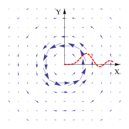
Figure 1: (color online) First-order paramagnetic current for light with $l=1$ and polarization $\sigma-$. The center of the plot coincides with the beam axis. The factor $J_{m-l}(k_{r}^{\prime}r)J_{m}(k_{r}r)$ is drawn in dashed (red) line.

Interband-coherence contribution: The interband-coherence contribution to the current density is given by

$$\overline{\mathbf{j}}^{(coh)}(\mathbf{r},t) = \frac{2\,q}{m_{e}}\sum_{\scriptsize\begin{array}[]{c}\mathbf{k}^{\prime}m^{\prime}\\ \mathbf{k}m\end{array}}\Re\Big{[}\mathbf{p}_{vc}\,{\cal N}^{\prime}{\cal N}J_{m^{\prime}}(k_{r}^{\prime}r)J_{m}(k_{r}r)\times$$

$$\left.e^{i(k_{z}-k_{z}^{\prime})z}e^{i(m-m^{\prime})\phi}\rho_{v\mathbf{k}^{\prime}m^{\prime},c\mathbf{k}m}^{(1)}(t)\right]\,\,.$$

With the help of Eqs. (III.2) and (16) we simplify this expression to

$$\overline{\mathbf{j}}^{(coh)}(\mathbf{r},t) = \frac{2\,q}{m_{e}}\Re\Bigg{[}\mathbf{p}_{vc}e^{iq_{z}z}e^{il\phi}\sum_{\scriptsize\begin{array}[]{c}k_{r}^{\prime}k_{r}\\ k_{z}m\end{array}}{\cal N}^{\prime}{\cal N}\times$$

$$\left.J_{m-l}(k_{r}^{\prime}r)J_{m}(k_{r}r)\,\rho_{vk_{z}-q_{z}k_{r}^{\prime}m-l,ck_{z}k_{r}m}^{(1)}(t)\right]\,.$$

Figure 2: (color online) First-order paramagnetic current for light with $l=1$. The center of each plot coincides with the beam axis. Each panel pictures a different slice along the $z$-axis, showing the wave nature and space variation of the pattern.

The main feature of this expression is that it contains a sum over products of space- and time-dependent functions. The time dependence presents two distinct scales, as mentioned before: a rapid oscillation related to the frequency $\omega$ of the light beam, and a slower one that is related to the detuning.

To describe the electric-current patterns in the plane perpendicular to the $z$-axis, we disregard the slow time evolution and focus on the space- and time-dependent quantity $\Re[\mathbf{p}_{vc}e^{i(q_{z}z+l\phi-\omega t)}J_{m-l}(k_{r}^{\prime}r)J_{m}(k_{r}r)]$, see Fig. 1. We can see that the current density and the angular momentum at this level are consistent with each other. To see this, let us take as an example a TL field having circular polarization $\sigma_{+}=\hat{x}+i\hat{y}$. From the usual selection rule for the absorption of a photon, a non-vanishing light-matter matrix element requires $\mathbf{p}_{cv}=p_{0}(\hat{x}-i\hat{y})$. Since $\mathbf{p}_{vc}=\mathbf{p}_{cv}^{*}=p_{0}(\hat{x}+i\hat{y})$, we see from Eq. (24) that a non-vanishing angular momentum will appear only if $l=-1$; in this case the current pattern reflects this fact, presenting a “circulation” around the beam axis. On the contrary, if the beam is tuned to $l=+1$ and $\sigma+$, the current forms a pattern that does not “flow” around the axis. As we move along the $z$-axis for fixed time, we observe the wave nature of the x-y plane current (Fig. 2). For fixed $z$, the wave nature is revealed as time evolves. For different values of $l$, the electric current develops more complex patterns, which mimic the complex structure of the electric field of a TL beam. In the case of $|l|>1$, there appear more than one off-centered vortices, as illustrated in Fig. 3.

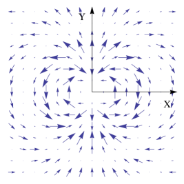
Figure 3: (color online) First-order paramagnetic current for light with $l=2$. The center of the plot coincides with the beam axis. The space pattern is more complex than in the $l=1$ case and exhibits circulation around off-axis centers.

From the above we can extract some general features of $\overline{\mathbf{j}}^{(coh)}(\mathbf{r},t)$. Driven by the interband coherence, it oscillates in time, with zero mean, at the frequency of the EM field, and presents complex spatial patterns that are related to the peculiar electric field of the TL beam. For special cases, the spatial pattern displays a circulation (of microscopic origin and not to be confused with a macroscopic excursion of the electrons around the beam axis) related to the non-vanishing coherence contribution of angular momentum calculated in Sec. IV.1.

Population and intraband-coherence contribution: The population and intraband-coherence contribution to the paramagnetic current is given by

$$\overline{\mathbf{j}}^{(pop)}(\mathbf{r},t) = -i\,\frac{q\,\hbar}{2\,m_{e}}\sum_{\scriptsize\begin{array}[]{c}\mathbf{k}^{\prime}m^{\prime}\\ \mathbf{k}m\end{array}}\left\{[\Phi_{\mathbf{k}^{\prime}m^{\prime}}^{*}(\mathbf{r})\nabla\Phi_{\mathbf{k}m}(\mathbf{r})]-\right.$$

$$\left.[\Phi_{\mathbf{k}m}(\mathbf{r})\nabla\Phi_{\mathbf{k}^{\prime}m^{\prime}}^{*}(\mathbf{r})]\right\}\,\rho_{c\mathbf{k}^{\prime}m^{\prime},\mathbf{k}m}^{(2)}(t)+\{c\rightarrow v\}\,,$$

where $\rho_{c\mathbf{k}^{\prime}m^{\prime},\mathbf{k}m}^{(2)}(t)$ is given by Eqs. (19) and (21), and $\{c\rightarrow v\}$ stands for a similar term replacing $c$ by $v$. The intraband current in the direction of $\hat{\phi}$ is

$$\overline{j}^{(pop)}_{\phi}(\mathbf{r},t) = \frac{q\,\hbar}{m_{e}}\!\!\sum_{\scriptsize\begin{array}[]{c}k_{r}^{\prime}k_{r}\\ mk_{z}\end{array}}{\cal N}^{\prime}{\cal N}m\,\frac{1}{r}J_{m}(k_{r}^{\prime}r)J_{m}(k_{r}r)\times$$ (39)

$$\rho_{ck_{r}^{\prime}k_{z}m,k_{r}k_{z}m}^{(2)}(t)+\{c\rightarrow v\}\,.$$

Given that the electrons excited by the TL beam occupy initially a portion of the valence band that is symmetric with respect to the $\Gamma$ point of the Brillouin zone, we have disregarded the contribution to $\overline{j}^{(pop)}_{\phi}(\mathbf{r},t)$ coming from the holes left behind, and kept only the current produced by the imbalance of electrons in the conduction band. The parameter $l$ does not appear explicitly, but it enters $\rho_{ck_{r}^{\prime}k_{z}m,k_{r}k_{z}m}^{(2)}(t)$, since an electron leaving a state with $\{v,m\}$ goes to a state with $\{c,m+l\}$.

IV.2.2 Diamagnetic current density

Starting from Eq. (32), we perform a space average and obtain for the diamagnetic term

$$\mathbf{j}^{(d)}(\mathbf{r},t) = -\,\frac{q}{m_{e}}\mathbf{A}(\mathbf{r},t)\sum_{\scriptsize\begin{array}[]{c}k_{r}^{\prime}k_{r}\\ k_{z}m\end{array}}{\cal N}^{\prime}{\cal N}J_{m}(k_{r}^{\prime}r)J_{m}(k_{r}r)\times$$

$$\rho_{ck_{r}^{\prime}k_{z}m,k_{r}k_{z}m}^{(2)}(t)+\{c\rightarrow v\}\,,$$

We point out the following features of the diamagnetic current density: $i)$ it arises from populations and intraband coherences in each band; $ii)$ its vectorial character is given by the polarization of the light; $iii)$ it is of third order in the vector potential amplitude; $iv)$ it does not arise from an imbalance of the conduction-band population [it is not proportional to $m$ like $\overline{j}^{(pop)}_{\phi}(\mathbf{r},t)$, see Eq. (39)]; $v)$ its time evolution is given by the slow evolution of $\rho_{c}^{(2)}(t)$ and the fast oscillation of the field $\mathbf{A}(\mathbf{r},t)$.

V Conclusions

We developed a theory of the band-to-band transitions induced by twisted light (light carrying orbital angular momentum) in bulk semiconductors. We posed the problem of the light-matter interaction in terms of Heisenberg equations of motion for the populations and quantum coherences of a two-band semiconductor model, as customarily done. We found that the resulting system of equations is greatly simplified when the envelope electron wave functions are represented in cylindrical coordinates, instead of using the usual (cartesian) Bloch state representation. This simplification is due to the decoupling of the system of equations in subsystems determined by the orbital angular momentum of electrons. Though non-standard for the bulk case, our choice of basis states is, on the one hand, perfectly admissible and, on the other, it proves to be the best choice from a mathematical point of view. It is admissible because the material properties are unaffected by surface effects in the limit of a bulk/large system. It is the right choice since it provides the highest symmetry compatibility between the twisted-light vector potential and the electron states.

Despite the achieved simplification, the evolution of the different relevant physical quantities under the excitation by a time-dependent pulse must be computed via numerical analysis of the equations of motion. This task is left for future work; instead, we showed here analytical results in the low-excitation or perturbative regime. With the solutions for the populations and quantum coherences, we confirmed on more solid grounds our previous findings, i.e. that the optical excitation will generate electric currents, and that there will be a transfer of orbital angular momentum from the light beam to the electrons. Our analysis of the electric current and electron’s orbital angular momentum showed that two qualitatively different contributions enter both observables; they may be termed microscopic and macroscopic contributions. The microscopic contribution relates to the interband coherence and mimics the behavior of the electric field; from this and other reasons, it parallels the induced polarization of a semiconductor in the presence of plane-waves, as traditionally studied using the vertical-transition assumption. On the other hand, the macroscopic contribution signals a net transfer of OAM from the field to the electrons, and it parallels the photon-drag effect. We showed that the electric current exhibits a high degree of spatial complexity, due to the inhomogeneous nature of the twisted-light beam. Additionally, we have calculated and briefly analyzed the diamagnetic current, not addressed in our previous study.

Appendix A Particle in a hollow cylinder

We present the complete derivation of the electronic states in cylindrical coordinates, starting from the well-known solution of the Schrödinger equation without potential

$$-\frac{\hbar^{2}}{2m}\nabla^{2}\Phi(\mathbf{r})=E\Phi(\mathbf{r})\,,$$

where the Laplacian in cylindrical coordinates is

$$\nabla^{2}f=\frac{1}{r}\frac{\partial}{\partial r}\left(r\frac{\partial f}{\partial r}\right)+\frac{1}{r^{2}}\frac{\partial^{2}f}{\partial\theta^{2}}+\frac{\partial^{2}f}{\partial z^{2}}\,.$$

Consider a solution of the separable form $\Phi(\mathbf{r})=R(r)\Theta(\theta)Z(z)$; replacing into the Schrödinger equation, we get

$$-\frac{\hbar^{2}}{2m}\left[{1\over R}{1\over r}{\partial\over\partial r}\left(r{\partial R\over\partial r}\right)+{1\over\Theta}{1\over r^{2}}{\partial^{2}\Theta\over\partial\theta^{2}}+{1\over Z}{\partial^{2}Z\over\partial z^{2}}\right]=E$$

which yields

$$\left[{1\over R}{1\over r}{\partial\over\partial r}\left(r{\partial R\over\partial r}\right)+{1\over Z}{\partial^{2}Z\over\partial z^{2}}\right]+{1\over\Theta}{1\over r^{2}}{\partial^{2}\Theta\over\partial\theta^{2}} = -\alpha^{2}$$

where $\frac{2m}{\hbar^{2}}E=\alpha^{2}$. Then

$$\left[{1\over R}{r}{\partial\over\partial r}\left(r{\partial R\over\partial r}\right)+{r^{2}\over Z}{\partial^{2}Z\over\partial z^{2}}+\alpha^{2}r^{2}\right]+{1\over\Theta}{\partial^{2}\Theta\over\partial\theta^{2}} = 0\,,$$

which splits to

$${1\over R}{r}{\partial\over\partial r}\left(r{\partial R\over\partial r}\right)+{r^{2}\over Z}{\partial^{2}Z\over\partial z^{2}}+\alpha^{2}r^{2} = m^{2}$$

$${1\over\Theta}{\partial^{2}\Theta\over\partial\theta^{2}} = -m^{2}\,.$$

The second equation has solution $\Theta=A_{1}e^{im\theta}+A_{2}e^{-im\theta}$. The remaining equation is

$${1\over R}{1\over r}{\partial\over\partial r}\left(r{\partial R\over\partial r}\right)+\alpha^{2}-{m^{2}\over r^{2}}+{1\over Z}{\partial^{2}Z\over\partial z^{2}} = 0\,.$$

This is again separable

$${1\over R}{1\over r}{\partial\over\partial r}\left(r{\partial R\over\partial r}\right)+\alpha^{2}-{m^{2}\over r^{2}} = \lambda^{2}$$

$${1\over Z}{\partial^{2}Z\over\partial z^{2}} = -\lambda^{2}\,,$$

with solution $Z=Be^{i\lambda z}$, and equation

$${1\over R}r{\partial\over\partial r}\left(r{\partial R\over\partial r}\right)+(\alpha^{2}-\lambda^{2})r^{2}-{m^{2}} = 0\,,$$

and developing the derivatives

$$r^{2}{d^{2}R\over dr^{2}}+r{dR\over dr}+\left[(\alpha^{2}-\lambda^{2})r^{2}-{m^{2}}\right]R = 0\,,$$

which is almost the Bessel differential equation. Defining $x^{2}=(\alpha^{2}-\lambda^{2})r^{2}$ the correct differential equation follows

$$x^{2}{d^{2}R\over dx^{2}}+x{dR\over dx}+\left(x^{2}-{m^{2}}\right)R = 0\,.$$

A.1 Boundary conditions

For $Z(z)$ we use boundary conditions $Z(0)=Z(H)$, and obtain

$$Z(z) = {1\over\sqrt{H}}\,e^{i\lambda z}$$

$$\lambda = {2\pi n\over H}\,.$$

For $\Theta(\theta)$, the periodicity implies

$$\Theta(\theta) = N_{\theta}\,e^{im\theta}$$

$$m = \ldots,-2,-1,0,1,2,\ldots\,.$$

For the radial solution, since it has to be finite at the origin, the solutions are the Bessel functions of the first kind $J_{m}(x)$. If we demand that $J_{m}(x=\sqrt{\alpha^{2}-\lambda^{2}}L)=0$, then the $s$th zero $r_{ms}$ of the Bessel function should be $\alpha^{2}={(r_{ms}/L)^{2}+\lambda^{2}}$:

$$E_{nms} = \frac{\hbar^{2}}{2m}\left[\left(\frac{r_{ms}}{L}\right)^{2}+\left(\frac{2\pi n}{H}\right)^{2}\right]$$

$$\Phi_{nms}(\mathbf{r}) = {\cal N}_{ms}J_{m}(\sqrt{\alpha^{2}-\lambda^{2}}\,r)e^{im\theta}e^{i{2\pi n\over H}z}\,,$$

with normalization ${\cal N}_{ms}=\frac{2}{LJ_{m}^{\prime}(r_{ms})}\sqrt{\frac{1}{2\pi\,H}}$, and $\lambda<\alpha$ for any admissible solution.

A.2 Cylinder with a Bravais lattice

In the effective-mass approximation, the complete wave function is expressed as the product of an envelope $\Phi_{nms}(\mathbf{r})$ and a periodic $u(\mathbf{r})$ function. Then, the Schrödinger equation reads

$$-\frac{\hbar^{2}}{2m}u(\mathbf{r})\nabla^{2}\Phi_{nms}(\mathbf{r})-\frac{\hbar^{2}}{2m}\Phi_{nms}(\mathbf{r})\nabla^{2}u(\mathbf{r})-$$

$$\frac{\hbar^{2}}{m}[\nabla\Phi_{nms}(\mathbf{r})]\cdot[\nabla u(\mathbf{r})]+U(\mathbf{r})[\Phi_{nms}(\mathbf{r})u(\mathbf{r})]=$$

$$E\Phi(\mathbf{r})u(\mathbf{r})\,,$$

where $U(\mathbf{r})$ is the lattice potential. Since we have already solved the problem of the free particle without $u(\mathbf{r})$, we know that $-\frac{\hbar^{2}}{2m}\nabla^{2}\Phi_{nms}(\mathbf{r})=E^{(0)}_{nms}\Phi_{nms}(\mathbf{r})$. Dividing by $\Phi_{nms}(\mathbf{r})$ and grouping terms we get

$$-\frac{\hbar^{2}}{2m}\nabla^{2}u(\mathbf{r})+U(\mathbf{r})u(\mathbf{r})-\frac{\hbar^{2}}{m}\frac{\nabla\Phi_{nms}(\mathbf{r})\cdot\nabla u(\mathbf{r})}{\Phi_{nms}(\mathbf{r})}$$

$$=(E-E^{(0)}_{nms})u(\mathbf{r})\,.$$

This is an equation for $u(\mathbf{r})$ [since we already know the functional form of $\Phi_{nms}(\mathbf{r})$]. We ask that $u(\mathbf{r})=u(\mathbf{r}+\mathbf{R})$, with $\mathbf{R}$ a lattice vector, so we can regard the region of integration as the unit cell. Then, if $\Phi_{nms}$ varies slowly in the unit cell, we see $(\hbar^{2}/m)\Phi_{nms}(\mathbf{r})^{-1}[\nabla\Phi_{nms}(\mathbf{r})]\cdot[\nabla u(\mathbf{r})]$ as a perturbation. This is simply the $\bf k\cdot p$ approximation in a different coordinate system. To lowest order we have

$$-\frac{\hbar^{2}}{2m}\nabla^{2}u(\mathbf{r})+U(\mathbf{r})u(\mathbf{r}) = \Delta E\,u(\mathbf{r})\,,$$

and from here one obtains $u(\mathbf{r})$ as usual. Therefore, we take the eigenfunctions as a product of envelope and periodic functions, while the energy is that of the envelope corrected by the energy gap and the effective mass:

$$E_{bnms} = \frac{\hbar^{2}}{2m_{b}^{*}}\left[\left(\frac{r_{ms}}{L}\right)^{2}+\left(\frac{2\pi n}{H}\right)^{2}\right]+\delta_{bc}E_{g}$$

$$\Psi_{bnms}(\mathbf{r}) = \frac{N_{r}}{\sqrt{2\pi H}}J_{m}[({r_{ms}/L})\,r]e^{im\theta}e^{i{2\pi n\over H}z}u_{b}(\mathbf{r})\,,$$

where $H$ is the height and $L$ the radius of the cylinder.

References

• (1) L. Allen, M. W. Beijersbergen, R. J. C. Spreeuw, and J. P. Woerdman, Phys. Rev. A 45, 8185 (1992).
• (2) David L. Andrews, Structured Light and Its Applications: An Introduction to Phase-Structured Beams and Nanoscale Optical Forces (Academic Press, 2008).
• (3) S. J. Van Enk and G. Nienhuis, J. Modern Optics 41, 963 (1994).
• (4) L. Allen and M. J. Padgett, Optics Communications 184, 67 (2000).
• (5) G. Molina-Terriza1, J. P. Torres, and L. Torner, Nature Physics 3, 305 (2007).
• (6) B. L. C. Dávila-Romero, D. L. Andrews, and M. Babiker, J. Opt. B. Quantum Semiclass. Opt. 4, S66-S72 (2002).
• (7) S. Barreiro and J. W. R. Tabosa, Phys. Rev. Lett.  90, 133001 (2003).
• (8) M. E. J. Friese, T. A. Nieminen, N. R. Heckenberg, and H. Rubinsztein-Dunlop, Nature 394, 348 (1998).
• (9) M. Babiker, C. R. Bennett, D. L. Andrews, and L. C. Dávila Romero, Phys. Rev. Lett. 89, 143601 (2002).
• (10) V. Garcés-Chávez, K. Volke-Sepulveda, S. Chávez-Cerda, W. Sibbett, and K. Dholokia, Phys. Rev. A 66, 063402 (2002).
• (11) F. Araoka, T. Verbiest, K. Clays, and A. Persoons, Phys. Rev. A 71, 055401 (2005).
• (12) T. P. Simula, N. Nygaard, S. X. Hu, L. A. Collins, B. I. Schneider, and K. Mølmer, Phys. Rev. A 77, 015401 (2008).
• (13) O. Hess and T. Kuhn, Phys. Rev. A 54, 3347 (1996).
• (14) F. Rossi and T. Kuhn, Rev. Mod. Phys. 74, 895 (2002).
• (15) M. Herbst, M. Glanemann, V. M. Axt, and T. Kuhn, Phys. Rev. B 67, 195305 (2003).
• (16) G. F. Quinteiro and P. I. Tamborenea, EPL 85, 47001 (2009).
• (17) H. Haug and Anti-Pekka Jauho, Quantum Kinetics in Transport and Optics of Semiconductors, (Springer, Berlin, Heidelberg, 1996).
• (18) A. F. Gibson and C. Walker, J. Phys. C:Solid State Phys. 4, 2209 (1971).
• (19) A. F. Gibson and S. Montasser, J. Phys. C:Solid State Phys. 8, 3147 (1975).
• (20) G. F. Quinteiro and P. I. Tamborenea, Phys. Rev. B 79, 155450 (2009).
• (21) G. F. Quinteiro and J. Berakdar, Opt. Express 17, 20465-20475 (2009).
• (22) R. Jáuregui, Phys. Rev. A 70, 033415 (2004).
• (23) Claude Cohen-Tannoudji, Jacques Dupont-Roc, Gilbert Grynberg, Photons and Atoms, Introduction to Quantum Electrodynamics, (John Wiley & Sons, New York, 1997).
• (24) A. S. Moskalenko, A. Matos-Abiague, and J. Berakdar Phys. Rev. B 74, 161303(R) (2006).
• (25) Harald Ibach and Hans Lüth, Solid-State Physics, An Introduction to Principles of Materials Science, Second Edition (Springer-Verlag Berlin Heidelberg, 1995).
• (26) H. Haug and S. W. Koch, Quantum theory of the optical and electronic properties of semiconductors, Fourth Edition (World Scientific Publishing Co., 2004).