Detection of relic gravitational waves in the CMB: Prospects for CMBPol mission

Abstract

Detection of relic gravitational waves, through their imprint in the cosmic microwave background radiation, is one of the most important tasks for the planned CMBPol mission. In the simplest viable theoretical models the gravitational wave background is characterized by two parameters, the tensor-to-scalar ratio $r$ and the tensor spectral index $n_{t}$. In this paper, we analyze the potential joint constraints on these two parameters, $r$ and $n_{t}$, using the potential observations of the CMBPol mission, which is expected to detect the relic gravitational waves if $r\gtrsim 0.001$. The influence of the contaminations, including cosmic weak lensing, various foreground emissions, and systematical errors, is discussed.

I Introduction

The detection of primordial gravitational waves is rightly considered a highest priority task for the upcoming observation missions task . A stochastic background of the relic gravitational waves (RGWs), produced in the very early Universe due to the superadiabatic amplification of zero point quantum fluctuations of the gravitational field, is a necessity dictate by general relativity and quantum mechanics grishchuk . So the detection of RGWs maybe provide the unique way to study the birth of the Universe, and test the applicability of general relativity and quantum mechanics in the very high energy scale a12a .

In a whole range of scenarios of the early Universe, the primordial power spectrum of the RGWs can be well described by a power-law form in a fairly large frequency range a2a ; a2 ; a3 ; a4 ; zhao ; others . Thus, the RGW backgrounds are conventionally simply characterized by two parameters, the so-called tensor-to-scalar ratio $r$ and the primordial power spectral index of RGWs $n_{t}$, where $r$ describes the amplitude of the primordial spectrum, and $n_{t}$ denotes the tilt of the spectrum. So the constraints on $r$ and $n_{t}$ will give us a direct glimpse into the physical conditions in the early Universe. In particular, they will allow us to place the constraints on the Hubble parameter of the early Universe, and time evolution of this Hubble parameter. Unfortunately, the models of the early Universe cannot give a definite prediction for the values of $r$ and $n_{t}$, i.e., different inflationary models predict the quite different values of $r$ and $n_{t}$ liddle , especially some string motivated inflationary models predict a very small gravitational waves with $r\ll 10^{-4}$ string . So, the only way to determine them is by the observations.

The RGWs leave well understood imprints on the anisotropies in temperature and polarization of cosmic microwave background radiation (CMB) polnarev ; a8 ; a10 ; a11 ; a13 ; polnarevTE ; zbgte . More specifically, RGWs produce a specific pattern of polarization in the CMB known as the $B$-mode polarization a8 . Moreover, RGWs produce a negative cross-correlation between the temperature and polarization known as the $TE$-correlation at the low multipoles $\ell\lesssim 50$ polnarevTE ; zbgte . The theoretical analysis of these imprints along with the data from CMB experiments allows to place constraints on the parameters $r$ and $n_{t}$ describing the RGW background, which provides the unique way to detect the RGWs at the very low frequencies ($10^{-17}\sim 10^{-15}$ Hz).

The current CMB experiments are yet to detect a definite signature of RGWs currentconstraint , although a hint of RGWs is found in the WMAP data zbghint . A number of authors have discussed the possibility of RGW detection by the launched Planck satellite Planck ; z ; zbghint ; ma . The results show that, due to the fairly large instrumental noises, only if the tensor-to-scalar ratio is large ($r\gtrsim 0.05$), the Planck satellite is expected to have a detection. In the previous paper zb , we also found that the Planck mission cannot give a good constraint for the spectral index $n_{t}$, even if the tensor-to-scalar ratio is as large as $r=1$. In addition, various ground-based groundbasedCMB and balloon-borne balloonbasedCMB CMB experiments are expected to have the better detection abilities, which can constrain the parameter $r$ fairly well when $r\gtrsim 0.01$. However, an accurate constraint of $n_{t}$ is still unexpected, due to the small partial sky observation or the short time observation zz .

The accurate determination of the RGWs requires the full sky and the long time observations by the CMB experiment with the quite small instrumental noises. The future space-based mission focus on the CMB polarization cmbpol (here and in the following, we use the label ‘CMBPol’ to refer it) provides an excellent opportunity to realize it (the similar projects, such as B-Pol b-pol and LiteBird litebird , are also proposed). The instrumental noises of CMBPol mission are more than $100$ times smaller than those of Planck mission. If the foreground contaminations and the systematical errors can be well controlled, the signature of RGWs can be well detected, as long as $r\gtrsim 0.001$ cmbpol . This will provide an observational tool to distinguish the different inflationary-type models.

In this paper we shall analyze the joint constraints on two parameters $r$ and $n_{t}$ that would be feasible with the analysis of the observations from the planned CMBPol mission. We shall detailedly discuss the constraints of $r$, $n_{t}$ and the best-pivot wavenumber $k_{t}^{*}$ depending on the input (or true) value of the tensor-to-scalar ratio $r$. We discuss the effects of various contaminations from the cosmic weak lensing, foreground radiations and the beam systematics.

The outline of the paper is as follows. In Sec. II we shall introduce and explain the notations for the power spectra of gravitational waves, density perturbations and various CMB anisotropy fields. Furthermore, in this section, we shall briefly introduce the existence of the best-pivot wavenumber $k_{t}^{*}$ for the detection of RGWs in the CMB. The analytical formulae and explanation for the $k_{t}^{*}$, $\Delta r$ and $\Delta n_{t}$ will also be discussed. In Sec. III, by using the analytical formulae and only considering the instrumental noises, we shall discuss the values of $k_{t}^{*}$, $\Delta r$ and $\Delta n_{t}$ for different input (or true) value of $r$. Sec. IV is contributed to show the effect of the cosmic lensing contamination, and Sec. V is contributed to show the effect of the foreground radiations contamination. In Sec. VI, we discuss the effects of various beam systematics for the determination of the parameters $r$ and $n_{t}$. We also discuss the requirement of the CMBPol’s systematics, if the biases of the parameters $r$ and $n_{t}$ are ignorable. Finally, Sec. VII is dedicated to a brief discussion and conclusion.

II Optimal parameters and their determinations

The main contribution to the observed temperature and polarization anisotropies of the CMB comes from two types of the cosmological perturbations, density perturbations (also known as the scalar perturbations) and RGWs (also known as the tensor perturbations) polnarev ; a3 ; a4 ; a8 , which are generally characterized by their primordial power spectra. These power spectra are usually assumed to be power-law, which is a generic prediction of a wide range of scenarios of the early Universe, including the inflationary models. In general there might be deviations from a power-law, which can be parameterized in terms of the running of the spectral index (see for example GrishchukSolokhin ; liddle ), but we shall not consider this possibility in the current paper. Thus, the power spectra of the perturbation fields have the form

$$P_{s}(k)=A_{s}(k_{0})(k/k_{0})^{n_{s}-1},~{}~{}~{}~{}P_{t}(k)=A_{t}(k_{0})(k/k_{0})^{n_{t}},$$ (1)

for density perturbations and RGWs respectively. In the above expression $k_{0}$ is an arbitrarily chosen pivot wavenumber, $n_{s}$ is the primordial power spectral index for density perturbations, and $n_{t}$ is the primordial power spectral index for RGWs. $A_{s}(k_{0})$ and $A_{t}(k_{0})$ are normalization coefficients determining the absolute values of the primordial power spectra at the pivot wavenumber $k_{0}$. The choices of $n_{s}=1$ and $n_{t}=0$ correspond to the scale-invariant power spectra for density perturbations and gravitational waves respectively.

The relative contribution of density perturbations and gravitational waves is described by the so-called tensor-to-scalar ratio $r$, which is defined as follows

$$r(k_{0})\equiv\frac{A_{t}(k_{0})}{A_{s}(k_{0})}.$$ (2)

Note that, in defining the tensor-to-scalar ratio $r$, we have not used any inflationary formulae which relate $r$ with the physical conditions during inflation and the slow-roll parameters (see for example stein ). Thus, our definition depends only on the power spectral amplitudes of density perturbations and RGWs, and does not assume a particular generating mechanism for these cosmological perturbations. The RGW amplitude $A_{t}\left(k_{0}\right)=r(k_{0})A_{s}(k_{0})$ provides us with direct information on the Hubble parameter of the very early Universe GrishchukSolokhin . More specifically, this amplitude is directly related to the value of the Hubble parameter $H$ at a time when wavelengths corresponding to the wavenumber $k_{0}$ crossed the horizon wmap_notation

$$A_{t}^{1/2}(k_{0})=\left.\frac{\sqrt{2}}{M_{\rm pl}}\frac{H}{\pi}\right|_{k_{0}/a=H},$$ (3)

where $M_{\rm pl}=1/\sqrt{8\pi G}$ is the reduced Planck mass. If we adopt $A_{s}=2.445\times 10^{-9}$ as predicted by the WMAP5 observations wmap5 , the Hubble parameter is $H\simeq 2.67r^{1/2}\times 10^{14}$GeV, only depending on the value of $r$. In the canonical single-field slow-roll inflationary models, the Hubble parameter directly relates to the energy scale of inflation $V^{1/4}$. The relation (3) follows that $V^{1/4}\simeq 3.35r^{1/4}\times 10^{16}$GeV, which has been emphasized by a number of authors.

Assuming that the amplitude of density perturbations $A_{s}(k_{0})$ is known, taking into account the definitions (1) and (2), the power spectrum of the RGW field may be completely characterized by tensor-to-scalar ratio $r$ and the spectral index $n_{t}$. It is important to mention that, for spectral indices different from the scale-invariant case (i.e., when $n_{s}\neq 1$ or/and $n_{t}\neq 0$), the definition of the tensor-to-scalar ratio depends on the pivot wavenumber $k_{0}$. If we adopt a different pivot wavenumber $k_{1}$, the tensor-to-scalar ratio at this new pivot wavenumber $r(k_{1})$ is related to original ratio $r(k_{0})$ through the following relation (which follows from the definitions (1) and (2))

$$r(k_{1})=r(k_{0})\left(\frac{k_{1}}{k_{0}}\right)^{n_{t}-n_{s}+1}.$$ (4)

Let us now turn our attention to CMB. Density perturbations and gravitational waves produce temperature and polarization anisotropies in the CMB, which are characterized by four angular power spectra $C_{\ell}^{T}$, $C_{\ell}^{C}$, $C_{\ell}^{E}$ and $C_{\ell}^{B}$ as functions of the multipole number $\ell$. Here $C_{\ell}^{T}$ is the power spectrum of the temperature anisotropies, $C_{\ell}^{E}$ and $C_{\ell}^{B}$ are the power spectra of the so-called $E$ and $B$ modes of polarization (note that, density perturbation do not generate $B$-mode of polarization a8 ), and $C_{\ell}^{C}$ is the power spectrum of the temperature-polarization cross correlation.

In general, the power spectra $C_{\ell}^{Y}$ (where $Y=T,E,B$ or $C$) can be presented in the following form

$$C_{\ell}^{Y}=C_{\ell}^{Y}({\rm dp})+C_{\ell}^{Y}({\rm gw}),$$ (5)

where $C_{\ell}^{Y}({\rm dp})$ is the power spectrum due to the density perturbations, and $C_{\ell}^{Y}({\rm gw})$ is the power spectrum due to RGWs. In the case of RGWs, the CMB power spectra can be presented in the following form a10 ; a11

$$C_{\ell}^{Y}({\rm gw}) = (4\pi)^{2}\int\frac{dk}{k}P_{t}(k)\left[\Delta^{(T)}_{Y\ell}(k)\right]^{2},~{}~{}{\rm for}~{}Y=T,E,B,$$

$$C_{\ell}^{C}({\rm gw}) = (4\pi)^{2}\int\frac{dk}{k}P_{t}(k)\left[\Delta^{(T)}_{T\ell}(k)\Delta^{(T)}_{E\ell}(k)\right].$$ (6)

The transfer functions $\Delta_{Y\ell}^{(T)}(k)$ (see a10 ; a11 for details) in the above expressions translate the power in the metric fluctuations (gravitational waves) into corresponding CMB power spectrum at an angular scale characterized by multipole $\ell$. In this work, for numerical evaluation of the CMB power spectra due to density perturbations and gravitational waves, we use the publicly available CAMB code camb .

Since we are primarily interested in the parameters of the RGW field, in the analytical and numerical analysis below we shall work with a fixed cosmological background model. More specifically, we shall work in the framework of $\Lambda$CDM model, and keep the background cosmological parameters fixed at the values determined by a typical model wmap5

$$h=0.705,~{}\Omega_{b}h^{2}=0.02267,~{}\Omega_{m}h^{2}=0.1131,~{}\Omega_{k}=0,~{}\tau_{reion}=0.084,~{}A_{s}=2.445\times 10^{-9}.$$ (7)

Furthermore, the spectral indices of density perturbations and gravitational waves are adopted as follows for the simplicity,

$$n_{s}=1,~{}~{}n_{t}=0.$$ (8)

Note that throughout this paper, we have considered the simplest cosmological model. In the more general consideration, one should also include the running of the spectral indices GrishchukSolokhin , the details of the reionization history mortonson and so on, which have been ignored in this paper.

The CMB power spectra $C_{\ell}^{Y}$ are theoretical constructions determined by ensemble averages over all possible realizations of the underlying random process. However, in real CMB observations, we only have access to a single sky, and hence to a single realization. In order to obtain information on the power spectra from a single realization, it is required to construct estimators of power spectra. In order to differentiate the estimators from the actual power spectra, we shall use the notation $D_{\ell}^{Y}$ to denote the estimators while retaining the notation $C_{\ell}^{Y}$ to denote the power spectrum. It is important to keep in mind that the estimators $D_{\ell}^{Y}$ are constructed from observational data, while the power spectra $C_{\ell}^{Y}$ are theoretically predicted quantities. The probability distribution functions for the estimators are described in detail in zbgte (see also z ; wishart2 ; pdf1 ), which predicts the expectation values of the estimators

$$\langle D_{\ell}^{Y}\rangle=C_{\ell}^{Y},$$ (9)

and the standard deviations

$$(\sigma_{D_{\ell}^{X}})^{2} = \frac{2(C_{\ell}^{X}+N_{\ell}^{X})^{2}}{(2\ell+1)f_{\rm sky}},~{}~{}(X=T,E,B)$$

$$(\sigma_{D_{\ell}^{C}})^{2} = \frac{(C_{\ell}^{T}+N_{\ell}^{T})(C_{\ell}^{E}+N_{\ell}^{E})+(C_{\ell}^{C}+N_{\ell}^{C})^{2}}{(2\ell+1)f_{\rm sky}},$$ (10)

where $f_{\rm sky}$ is the sky-cut factor. In this paper, we use $f_{\rm sky}=0.8$ for the CMBPol survey. $N_{\ell}^{Y}$ are the noise power spectra, which are all determined by the specific experiments. In this formulas, the possible bias generated by the beam systematics has not been considered (see Sec. VI for details).

In order to estimate the parameters $r$ and $n_{t}$ characterizing the RGW background, we shall use an analysis based on the likelihood function cosmomc . The likelihood function is just the probability density function of the observational data considered as a function of the unknown parameters (which are $r$ and $n_{t}$ in our case). Up to a constant, independent of its arguments, the likelihood function is given by

$$\mathcal{L}=\prod_{\ell}f(D_{\ell}^{C},D_{\ell}^{T},D_{\ell}^{E},D_{\ell}^{B}),$$

where the function $f(D_{\ell}^{C},D_{\ell}^{T},D_{\ell}^{E},D_{\ell}^{B})$ is explained in detail in the previous works z ; zb .

In the previous works z ; zb , we have discussed how to constrain the parameters of the RGWs, $r$ and $n_{t}$, by the CMB observation. In zb , we found that in general, the constraints on $r$ and $n_{t}$ correlate with each other. However, if we consider the tensor-to-scalar ratio at the best-pivot wavenumber $k_{t}^{*}$, i.e. $r^{*}\equiv r(k_{t}^{*})$, the constraints on $r$ and $n_{t}$ becomes independent of each other, and the uncertainties $\Delta{r}$ and $\Delta{n_{t}}$ have the minimum values. We have derived the formulae to calculate the quantities: the best-pivot wavenumber $k_{t}^{*}$, and the uncertainties of the parameters $\Delta r$ and $\Delta{n_{t}}$, which provides a simple and quick method to investigate the detection abilities of the future CMB observations. We shall briefly introduce these results in this section.

It is convenient to define the quantities as below,

$$a_{\ell}^{Y}\equiv\frac{C_{\ell}^{Y}({\rm gw})}{\sigma_{D_{\ell}^{Y}}},~{}~{}b^{*}_{\ell}\equiv\ln\left(\frac{\ell}{\ell_{t}^{*}}\right),~{}~{}d_{\ell}^{Y}\equiv\frac{D_{\ell}^{Y}-C_{\ell}^{Y}({\rm dp})}{\sigma_{D_{\ell}^{Y}}},$$ (11)

where $C_{\ell}^{Y}({\rm gw})$ is the CMB power spectrum generated by RGWs, and $\sigma_{D_{\ell}^{Y}}$ is the standard deviation of the estimator $D_{\ell}^{Y}$, which can be calculated by Eq. (10). We should notice that, the quantity $d_{\ell}^{Y}$ is dependent of random date $D_{\ell}^{Y}$. By considering the relations in (9) and (5), we can obtain that $\langle d_{\ell}^{Y}\rangle=a_{\ell}^{Y}$, which shows that $d_{\ell}^{Y}$ is an unbiased estimator of $a_{\ell}^{Y}$. $\ell_{t}^{*}$ is the so-called best-pivot multipole, which is determined by solving the following equation zb :

$$\sum_{\ell}\sum_{Y}a_{\ell}^{Y2}b_{\ell}^{*}=0.$$ (12)

So the value of $\ell_{t}^{*}$ depends on the cosmological model, the amplitude of RGWs, and noise power spectra by the quantity $a_{\ell}^{Y}$. The best-pivot wavenumber $k_{t}^{*}$ relates to $\ell_{t}^{*}$ by the approximation relation zb ,

$$k_{t}^{*}\simeq\ell_{t}^{*}\times 10^{-4}{\rm Mpc}^{-1}.$$ (13)

The numerical factor here mainly reflects the angular-diameter distance to the last scattering surface.

Once the value of $\ell_{t}^{*}$ is obtained, the uncertainties $\Delta r^{*}$ and $\Delta n_{t}$ can be calculated by the following simple formulae

$$\Delta r^{*}=r^{*}/\sqrt{\sum_{\ell}\sum_{Y}a_{\ell}^{Y2}},~{}~{}~{}~{}\Delta n_{t}=1/\sqrt{\sum_{\ell}\sum_{Y}(a_{\ell}^{Y}b_{\ell}^{*})^{2}}.$$ (14)

As usual, we can define the signal-to-noise ratio $S/N\equiv r^{*}/\Delta r^{*}$. Using (14), we get

$$S/N=\sqrt{\sum_{\ell}\sum_{Y}a_{\ell}^{Y2}}.$$ (15)

In the previous work zb , we found the uncertainty of $r(k_{0})$, the tensor-to-scalar ratio at the pivot wavenumber $k_{0}\neq k_{t}^{*}$, is larger than $\Delta r^{*}$. The value of $\Delta\ln r(k_{0})$ is fairly well approximated by the following formula

$$\Delta\ln r(k_{0})=\sqrt{(\Delta r^{*}/r^{*})^{2}+(\ln(k_{0}/k_{t}^{*})\Delta n_{t})^{2}}.$$ (16)

The smallest uncertainty on tensor-to-scalar ratio $r$ is achieved for the choice of the pivot scale at $k_{0}=k_{t}^{*}$. This justified the title ‘best’ pivot wavenumber for $k_{t}^{*}$. We should notice that the values of $k_{t}^{*}$, $S/N$, $\Delta\ln r$ and $\Delta n_{t}$ only depend on the input (or true) cosmological model, but not on the data $D_{\ell}^{Y}$. In Fig. 1, we plot the value of $\Delta\ln r(k_{0})$ as a function of the pivot scale $k_{0}$, where the input model has $r=0.3$, and the Planck instrumental noises are considered (see zb for details). As expected, when $k_{0}\gg k_{t}^{*}$ or $k_{0}\ll k_{t}^{*}$, the uncertainty becomes much larger than $\Delta r^{*}$.

The likelihood function in (II) has the maximum value at $(r^{*}_{\rm ML},n_{t{\rm ML}})$. The values of $r^{*}_{\rm ML}$ and $n_{t{\rm ML}}$ depend on the data $D_{\ell}^{Y}$, different from the value of $\Delta r^{*}$ and $\Delta n_{t}$. In the previous work zb , we found that the values of $r^{*}_{\rm ML}$ and $n_{t{\rm ML}}$ can be very well approximated by the follows

$$r^{*}_{\rm ML}=r^{*}\frac{\sum_{\ell}\sum_{Y}a_{\ell}^{Y}d_{\ell}^{Y}}{\sum_{\ell}\sum_{Y}a_{\ell}^{Y2}},~{}~{}~{}n_{t{\rm ML}}=n_{t}+\frac{\sum_{\ell}\sum_{Y}a_{\ell}^{Y}d_{\ell}^{Y}b_{\ell}^{*}}{\sum_{\ell}\sum_{Y}(a_{\ell}^{Y}b_{\ell}^{*})^{2}},$$ (17)

which depend on the data by the quantity $d_{\ell}^{Y}$. If the CMB estimator $D_{\ell}^{Y}$ is unbiased for $C_{\ell}^{Y}$, as discussed above, we have $\langle r^{*}_{\rm ML}\rangle=r^{*}$ and $\langle n_{t{\rm ML}}\rangle=n_{t}$, where Eq. (12) is used. These show that $r^{*}_{\rm ML}$ and $n_{t{\rm ML}}$ are the unbiased estimators for $r^{*}$ and $n_{t}$, respectively. However, when $D_{\ell}^{Y}$ is a biased estimator for $C_{\ell}^{Y}$, $r^{*}_{\rm ML}$ and $n_{t{\rm ML}}$ will also be the biased estimators for $r^{*}$ and $n_{t}$, respectively (see Sec. VI for details), which brings the errors for the detection of RGWs.

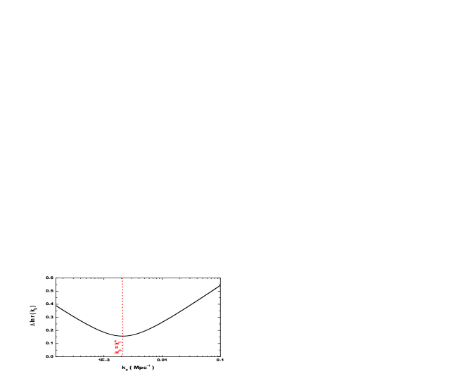
Figure 1: The uncertainty of $r(k_{0})$ for the different pivot wavenumber $k_{0}$.

The detection ability of the CMB experiment strongly depends on the noise levels, which include the instrumental noises, cosmic lensing contaminations, foreground radiation contaminations and the beam systematics. In the following sections, we shall discuss these effects separately. In addition, due to the partial sky survey, the leakage from the $E$-polarization into the $B$-polarization could be another kind of contamination. However, it was found that, this $E$-$B$ mixture can be properly avoided (or deeply reduced) by constructing the pure $E$-mode and $B$-mode polarization fields (see cutsky1 ; cutsky2 ; cutsky3 for details). So we shall not discuss this topic in this paper.

III CMBPol instrumental noises’ contaminations

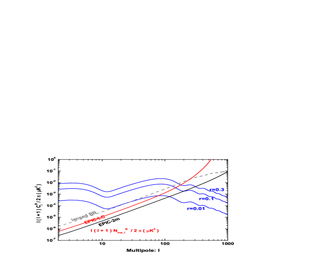
Figure 2: The instrumental noise power spectra $N_{{\rm ins},\ell}^{B}$ of EPIC-2m (black line) and EPIC-LC (red line).

Figure 3: The figures show the values of the best-pivot multipole $\ell_{t}^{*}$ (left panel), signal-to-noise ratio $S/N$ (middle panel) and the uncertainty of the RGW spectral index $\Delta n_{t}$ (right panel) as functions of $r^{*}$. The black solid (dash-dotted, dashed) lines correspond to the EPIC-2m instrumental noises (instrumental noises $+$ the reduced cosmic lensing contaminations, instrumental noises $+$ cosmic lensing contaminations), and the red solid (dashed) lines correspond to the EPIC-LC instrumental noises (instrumental noises $+$ the cosmic lensing contaminations).

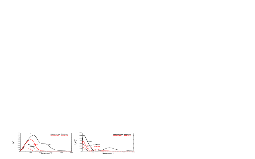
Figure 4: The figures show the values of $\sum_{Y}a_{\ell}^{Y2}$ (left panel) and $\sum_{Y}(a_{\ell}^{Y}b^{*}_{\ell})^{2}$ (right panel) as functions of multipole $\ell$ for the cases with the different $r^{*}$. Here, we have not considered the contaminations from cosmic weak lensing and foreground emissions.

Table 1: Experimental specifications for the mid-cost (EPIC-2m) CMBPol mission and the low-cost (EPIC-LC) CMBPol mission. cmbpol

	Frequency [GHz]	45	70	100	150	220
EPIC-2m	${\rm\theta}_{\rm F}$ [arcmin]	17	11	8	5	3.5
	$\Delta_{T}$ [${\rm\mu K}$-${\rm arcmin}$]	5.85	2.96	2.29	2.21	3.39
	Frequency [GHz]	40	60	90	135	200
EPIC-LC	${\rm\theta}_{\rm F}$ [arcmin]	116	77	52	34	23
	$\Delta_{T}$ [${\rm\mu K}$-${\rm arcmin}$]	15.27	8.23	3.56	3.31	3.48

In this section, we shall discuss the determination of RGWs, when only taking into account the instrumental noises of the CMBPol mission.

For a single frequency channel $i$, we assume Gaussian beams. The noise power spectrum (after deconvolution of the beam window function) is

$$N_{{\rm ins},\ell}^{T}(i)=(\Delta_{T})^{2}\exp\left[\frac{\ell(\ell+1)\theta_{F}^{2}}{8\ln 2}\right],~{}~{}N_{{\rm ins},\ell}^{C}(i)=0,$$ (18)

and

$$N_{{\rm ins},\ell}^{E}(i)=N_{{\rm ins},\ell}^{B}(i)=(\Delta_{P})^{2}\exp\left[\frac{\ell(\ell+1)\theta_{F}^{2}}{8\ln 2}\right],$$ (19)

where $\theta_{\rm F}$ is the full width at half maximum (FWHM) of the beam $i$. $\Delta_{T}$ and $\Delta_{P}$ are the noises for the temperature and polarizations, which relate by $\Delta_{P}=\sqrt{2}\Delta_{T}$. The values of the $\Delta_{T}$ and $\Delta_{P}$ depend on the number of the detectors, the integration time and the survey area.

If the experiment includes several different channels, we need to generalize the above considerations. The optimal channel combination of these channels gives the total effective instrumental noise cmbpol ,

$$[N_{{\rm ins},\ell}^{Y}]^{-1}=\sum_{i}\left[N_{{\rm ins},\ell}^{Y}(i)\right]^{-1},$$ (20)

where $i$ runs though the channels, $N_{{\rm ins},\ell}^{Y}(i)$ is the instrumental noise bias of the channel $\nu_{i}$. In this section, we shall only consider the instrumental noises, i.e.

$$N_{\ell}^{Y}\mapsto N^{Y}_{{\rm ins},\ell}.$$ (21)

Since the precise experimental specifications of CMBPol have not yet been defined, we will consider two different cases (EPIC-2m) and (EPIC-LC) suggested by cmbpol (recently, an EPIC-Intemediate Mission is also suggested by the CMBPol team cmbpol-middle ). The experimental specifications are given in Table 1, where 2-year design life is assumed . In Fig. 2, we plot the polarization noise spectra $N_{{\rm ins},\ell}^{B}$ of EPIC-2m and EPIC-LC, respectively . For EPIC-2m, when $\ell<100$, we find that $N_{{\rm ins},\ell}^{B}\sim 2.7\times 10^{-7}\mu$K², which is nearly $400$ times smaller than that of the Planck mission (7 frequency channels from $30$GHz to $353$GHz and $28$-month surveying time are assumed Planck ). Even for the EPIC-LC, when $\ell<100$, we have $N_{{\rm ins},\ell}^{B}\sim 6.2\times 10^{-7}\mu$K², $200$ times smaller than that of the Planck mission. So comparing with Planck mission, CMBPol is much more sensitive for the detection of CMB polarization. From Fig. 2, we also find that even for the model with quite small $r=0.01$, the value of $N_{{\rm ins},\ell}^{B}$ is smaller than that of $C_{\ell}^{B}$ when $\ell<120$ for EPIC-2m, and when $\ell<80$ for EPIC-LC. So the CMBPol mission provides an excellent opportunity to detailedly observe the peak of $C_{\ell}^{B}$ at $\ell\sim 80$.

Let us discuss the constraints on the gravitational waves by the potential observations of CMBPol mission. We shall discuss the values of the best-pivot scale $k_{t}^{*}$, the signal-to-noise ratio $S/N$ and the uncertainty of the spectral index $\Delta n_{t}$, by considering the CMBPol instrumental noises.

The value of $k_{t}^{*}$ directly relates to the best-pivot multipole $\ell_{t}^{*}$ by Eq.(13), and the value of $\ell_{t}^{*}$ is obtained by solving the equation in (12). By using (21), we obtain the value of $\ell_{t}^{*}$ as a function of the input (or true) value of the tensor-to-scalar ratio $r^{*}$ for EPIC-2m and EPIC-LC, which are plotted in Fig. 3 (left panel). We find that, in both cases, the value of $\ell_{t}^{*}$ becomes larger with the increasing of $r^{*}$. For EPIC-2m, we have $\ell_{t}^{*}=43$ for $r^{*}=0.001$, and $\ell^{*}_{t}=137$ for $r^{*}=0.1$. For EPIC-LC, the value of $\ell_{t}^{*}$ is smaller than that of EPIC-2m, due to the larger noise level and the larger beam FWHM of EPIC-LC. When $r=0.001$, we have $\ell_{t}^{*}=26$, and when $r=0.1$, we have $\ell_{t}^{*}=87$. These reflect that gravitational waves in the frequency range $k\sim 0.01$Mpc^-1 will be best constrained by the future CMBPol observations, unless the value of $r$ is extremely small. This is because the main contribution comes from the observation of the peak of $B$-polarization at $\ell\sim 80$. We should remember that this is different from the Planck case, where $\ell_{t}^{*}\sim 10$, due to the main contribution of the reionization peak of $B$-polarization zbgte ; z ; zb .

The signal-to-noise ratio is calculated by Eq. (15). By using Eq. (21), we get the value of $S/N$ as a function of $r^{*}$ for both EPIC-2m and EPIC-LC, which are shown in Fig. 3 (middle panel). As expected, the signal of RGWs can be very well determined by the CMBPol mission. Even for the model with $r=0.001$, we can have $S/N=19$ for EPIC-2m and $S/N=10$ for EPIC-LC, when only considering the corresponding instrumental noises. When $r=0.1$, we have $S/N=122$ for EPIC-2m and $S/N=81$ for EPIC-LC.

We can also calculate the value of $\Delta n_{t}$ by using Eq. (14) and the value of $\ell_{t}^{*}$ given in left panel of Fig. 3. The results are shown in Fig. 3 (right panel). As expected, the value of $\Delta n_{t}$ decreases with the increasing of $r^{*}$. For EPIC-2m, we have $\Delta n_{t}=0.06$ for the model with $r^{*}=0.001$, and $\Delta n_{t}=0.01$ for the model with $r^{*}=0.1$. This uncertainty is about $20$ times smaller than that given by Planck satellite zb ; zz . This constraint, combining with $\Delta r^{*}$, will give a quite sensitive way to differentiate various inflationary type models. For the EPIC-LC, the uncertainty of $n_{t}$ is about $2$ times larger that of EPIC-2m. When $r=0.001$, we have $\Delta n_{t}=0.10$, and when $r=0.1$, we have $\Delta n_{t}=0.02$.

It is necessary to discuss the contributions of $S/N$ and $\Delta n_{t}$ from every multipole, which can be very easily analyzed by the analytical formulae. From Eqs. (14) and (15), we find these two quantities can be rewritten as follows

$$(S/N)^{2}=\sum_{\ell}\sum_{Y}a_{\ell}^{Y2},~{}~{}~{}(1/\Delta n_{t})^{2}=\sum_{\ell}\sum_{Y}(a_{\ell}^{Y}b_{\ell}^{*})^{2}.$$ (22)

They are the simple sums of the contributions from each multipole $\ell$ and CMB information channel $Y$. We plot the functions of $\sum_{Y}a_{\ell}^{Y2}$ and $\sum_{Y}(a_{\ell}^{Y}b_{\ell}^{*})^{2}$ as a function of $\ell$ for two different models ($r=0.01$ and $r=0.1$). The results are shown in Fig. 4. Left panel shows that all these four lines are peaked at $\ell\sim 100$, which is close to the peak of $B$-polarization. This reflects that when $r>0.01$, the main contribution comes from the observation in the range $\ell\sim 100$, consistent with our previous discussion. This is different from the case of Planck satellite zbgte ; z , where the reionization peak at $\ell\sim 6$ is extremely important. In the CMBPol case, the contribution from the largest scale $\ell<20$ is unimportant due to the cosmic variance, and the contribution from the small scale $\ell>300$ is also unimportant for the large instrumental noises. However, it is important to mention that if $r\ll 0.01$, similar to Planck satellite, the reionization peak at $\ell<10$ again becomes the main contribution for the total $S/N$.

However, it is different for $\sum_{Y}(a_{\ell}^{Y}b_{\ell}^{*})^{2}$, which stands for the individual contribution for $1/\Delta n_{t}$. From the right panel of Fig. 4, we find that this function is sharply peaked at the largest scale $\ell<30$, and the contribution from intermedial scale around the best-pivot multpole is very small. These can be easily understood, the quantity $b_{\ell}^{*}\equiv\ln(\ell/\ell_{t}^{*})$ is zero when $\ell=\ell_{t}^{*}$, which follows that $\sum_{Y}(a_{\ell}^{Y}b_{\ell}^{*})^{2}=0$ at $\ell=\ell_{t}^{*}$. Only if $\ell\ll\ell_{t}^{*}$ or $\ell\gg\ell_{t}^{*}$, $b_{\ell}^{*}$ has a large value, and follows a large $\sum_{Y}(a_{\ell}^{Y}b_{\ell}^{*})^{2}$. Especially, the contribution from $\ell\ll\ell_{t}^{*}$ is very important. For example, when $\ell_{t}^{*}=137$, $b^{*2}_{\ell=2}$ is $30$ times large than $b^{*2}_{\ell=300}$. This reflects that the constraint on the tilt of the primordial gravitational waves power spectrum strongly depends on the observations in a large scale range. The cosmic reionization is very important for the constraint of $n_{t}$, although it might not be so important for the constraint of $r$ for the CMBPol observations.

IV Cosmic weak lensing contamination

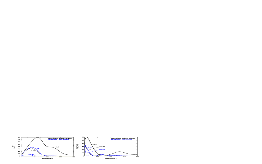
Figure 5: For EPIC-2m, the figures show the values of $\sum_{Y}a_{\ell}^{Y2}$ (left panel) and $\sum_{Y}(a_{\ell}^{Y}b^{*}_{\ell})^{2}$ (right panel) as functions of multipole $\ell$ for the cases with and without the reduced cosmic lensing contamination with the residual factor $\sigma^{\rm lens}=0.5$.

In a8 , it was pointed out that the gravitational waves result in CMB polarization with a $B$-mode, whereas density perturbations do not. Thus, the signal of gravitational waves could not be confused with density perturbations by detecting the $B$-polarization. Although, the amplitude of the $B$-polarization is expected to be quite small, it gives a clear information for gravitational waves. However, when taking into account the second-order effect, the $B$-mode can also arise from the lensing of the $E$-mode by density perturbations along lines-of-sight between the observer and the last-scattering surface lensing0 . The scalar contribution to the $B$-mode power spectrum is shown in Fig. 2 (grey dashed line). When $\ell<200$, it is nearly a white spectrum with the amplitude $C_{{\rm lens},\ell}^{B}\simeq 2\times 10^{-6}\mu$K², which is $7$ times larger than the instrumental noises of EPIC-2m, and $3$ times larger than that of EPIC-LC.

When the instrumental noise of the CMB experiment is sufficiently small, as the CMBPol mission, the gravitational lensing contribution to the large-scale $B$-mode becomes one of the limiting sources of contamination for constraining the RGWs. High-sensitivity measurements of small-scale $B$-modes can reduce this contamination through a lens reconstruction technique, which has been discussed by a number of authors (see for instance lensing1 ; lensing2 ; wuran4 ).

The effect of cosmic lensing contamination for the detection of RGWs can be easily discussed. The reduced lensed $B$-mode polarization can be treated simply as a well-known noise for gravitational waves in the likelihood analysis, i.e.

$$N_{\ell}^{B}\mapsto N_{{\rm ins},\ell}^{B}+C_{{\rm lens},\ell}^{B}\times\sigma^{\rm lens},$$ (23)

where we have defined the residual factor $\sigma^{\rm lens}$ for the lensed $B$-polarization. Note that in the real situation, the lens-induced $B$-modes are non-Gaussian, so we should not behave exactly it as the additional Gaussian noise (see wuran4 and references therein). However, on the scales relevant for $B$-mode detection in this paper, the non-Gaussianity has only a minor effect, which has been ignored in our discussion. In general, we have $\sigma^{\rm lens}\leq 1$, with the equality holding for the lensed $B$-mode is not reduced. The reduction of gravitational lensing contribution strongly depends on the instrumental noise level, the beam FWHM, the foregrounds and the instrumental systematics. In the work cmbpol-lensing , the authors found that, based on the noise level of EPIC-2m, one can expect to have $\sigma^{\rm lens}\sim 0.5$. However, for EPIC-LC, it is very difficult to reduce the cosmic lensing contamination due to the large beam FWHM. We should mention that since the value of $C_{{\rm lens},\ell}^{B}$ is much larger than the instrumental noises of CMBPol mission, in the total effective noise $N_{\ell}^{B}$, the cosmic lensing contamination becomes the dominant portion.

We have calculated the constraints of the gravitational waves by taking into account the cosmic lensing contaminations. The values of $\ell_{t}^{*}$, $S/N$ and $\Delta n_{t}$ are shown in Fig. 3, where $\sigma^{\rm lens}=0.5$ and $\sigma^{\rm lens}=1$ are considered for EPIC-2m, and $\sigma^{\rm lens}=1$ is considered for EPIC-LC. The left panel shows that, the best-pivot multipole is shifted to smaller scale by the lensing contamination. We find the value of $S/N$ is much reduced by the lensing contamination, especially for the case with small tensor-to-scalar ratio. When $r=0.001$, we have $S/N=7$ for EPIC-2m (with $\sigma^{\rm lens}=0.5$) and $S/N=4$ for EPIC-LC, which are much smaller than the corresponding values with only instrumental noises. The uncertainty of $n_{t}$ is also much increased by the cosmic lensing, especially for the case with small $r$. When $r=0.001$, EPIC-2m with $\sigma^{\rm lens}=0.5$ can give $\Delta n_{t}=0.12$, and EPIC-2m with $\sigma^{\rm lens}=1$ can give $\Delta n_{t}=0.16$, which are more than $2$ times larger than those in the case without cosmic lensing, and are fairly loose to differentiate various inflationary models. However, when the tensor-to-scalar ratio is $r=0.1$, we have $\Delta n_{t}=0.02$ for EPIC-2m, which is still a quite tight constraint.

We have also investigated the contribution of every multipole for $S/N$ and $\Delta n_{t}$. The results can be found in Fig. 5, where we have focused on the EPIC-2m mission and $\sigma^{\rm lens}=0.5$ is used for the case with cosmic lensing contamination. We find that the peak in each case is much reduced by the lensing contamination.

It is interesting to mention that for the high-sensitivity detectors the residual lensing noise dominates over the instrumental noises, and place the detection limit for CMB experiments song . In lensing2 , the authors claimed that, for a extreme high-sensitivity detector, a reduction in lensing power by a factor $40$ is possible using approximate iterative maximum-likelihood method. If we consider this residual as the lower limit of the reduced lensing noises, we find that $r>3.7\times 10^{-6}$ can be detected at more than $2$-$\sigma$ level in absence of sky cuts, foregrounds and instrumental systematics zb . This can be treated as the detection limit of the CMB experiments for gravitational waves. This lower limit corresponds to the Hubble parameter $H\simeq 3.1\times 10^{11}$GeV, and the energy scale of inflation $V^{1/4}\simeq 1.5\times 10^{15}$GeV. In this limit case, the uncertainty of spectral index also becomes very small. When $r=0.1$, we have $\Delta n_{t}=0.007$ (see Fig. 2 in zb for details), placing a very tight constraint on the inflationary models.

V Foreground contaminations

Table 2: Assumptions about foreground emissions. cmbpol

Parameter	Synchrotron	Dust
$A_{S,D}$	$4.7\times 10^{-5}$ $\mu$K2	$1.2\times 10^{-4}$ $\mu$K2
$\nu_{0}$	30 GHz	94 GHz
$\ell_{0}$	350	900
$\alpha$	-3	2.2
$\beta^{E}$	-2.6	-1.3
$\beta^{B}$	-2.6	-1.4
$\beta^{C}$	-2.6	-1.95

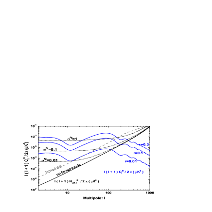
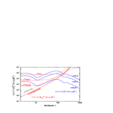
Figure 6: The total effective noise power spectra $N_{{\rm eff},\ell}^{B}$ when considering the foreground contaminations. The left panel is for EPIC-2m and the right panel is for EPIC-LC.

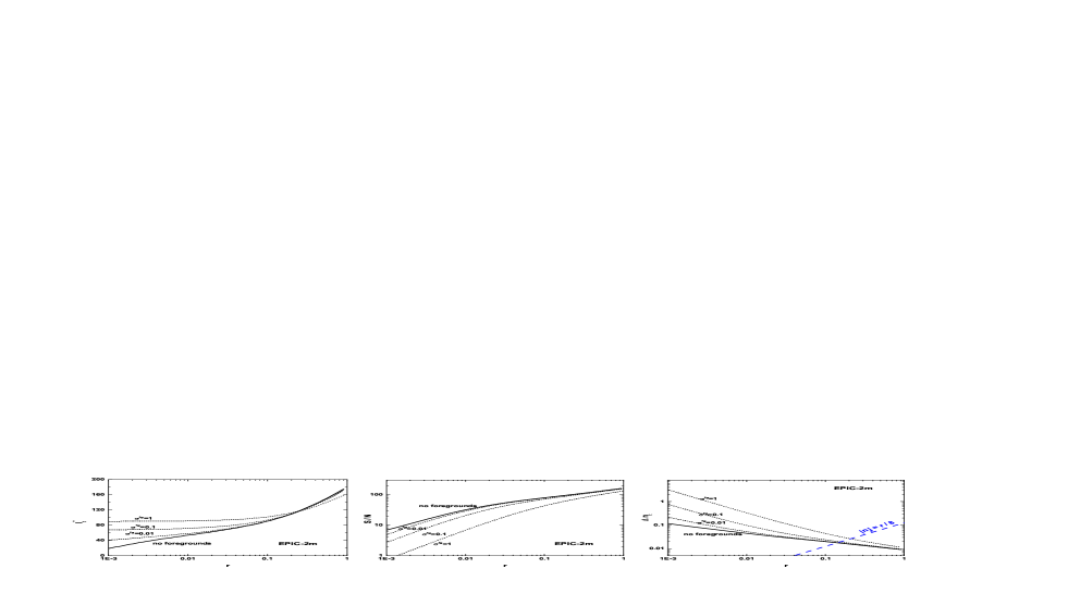
Figure 7: This figure shows the values of $\ell_{t}^{*}$, $S/N$ and $\Delta n_{t}$ depend on the foreground contaminations for EPIC-2m.

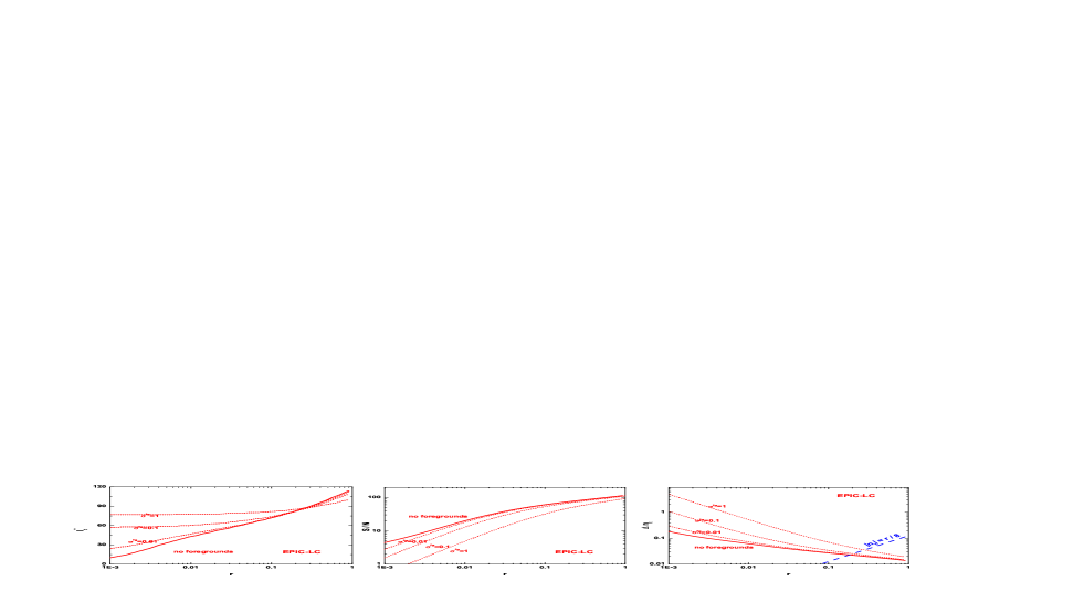
Figure 8: This figure shows the values of $\ell_{t}^{*}$, $S/N$ and $\Delta n_{t}$ depend on the foreground contaminations for EPIC-LC.

Figure 9: The figures show the values of $\sum_{Y}a_{\ell}^{Y2}$ (left panel) and $\sum_{Y}(a_{\ell}^{Y}b^{*}_{\ell})^{2}$ (right panel) as functions of multipole $\ell$ for the cases with different $\sigma^{\rm fg}$.

In this section, besides the instrumental noises and cosmic lensing contaminations, we shall take into account the impact of polarized foregrounds on the future CMBPol mission. In this paper, we shall neglect the effect of foregrounds on the CMB temperature, as the foreground cleaning is expected to leave a negligible contribution in the temperature bennett . CMB polarized foregrounds arise due to free-free, synchrotron, and dust emission, as well as due to extra-galactic sources such as radio sources and dusty galaxies. In this paper, we shall only consider only synchrotron and dust emission, which are expected to be dominant in the CMBPol frequency range cmbpol-fore .

The synchrotron emission results from the acceleration of cosmic-ray electrons in the magnetic field of Galaxy, which has been well measured on large angular scale at 23 GHz by WMAP. Following cmbpol ; verde ; cmbpol-fore , for the frequency $\nu$, the scale-dependence of the synchrotron signal may be parameterized as

$$C_{{\rm S},\ell}^{Y}(\nu)=A_{S}\left(\frac{\nu}{\nu_{0}}\right)^{2\alpha_{S}}\left(\frac{\ell}{\ell_{0}}\right)^{\beta^{Y}_{S}}.$$ (24)

The parameters in this formula for the various power spectra are all listed in Table 2, where $\alpha_{S}=-3$ is assumed, $\beta^{E}$, $\beta^{B}$ and $\beta^{C}$ are the corresponding $\beta^{Y}_{S}$ for synchrotron emissions. This choice matches the synchrotron emission at $23$GHz observed and parameterized by WMAP wmap-fore , and agrees with the DASI measurements dasi-fore .

Galactic emission in the $100-6000$ GHz frequency range is dominated by the thermal emission from warm interstellar dust grains. Our knowledge of polarized dust emission is relatively poor, which is expected to be characterized by the Planck satellite in the near future. In this paper, we shall adopt the parameterized formula for the dust emission at frequency $\nu$ as follows, as suggested by verde ; cmbpol ,

$$C_{{\rm D},\ell}^{Y}(\nu)=p^{2}A_{D}\left(\frac{\nu}{\nu_{0}}\right)^{2\alpha_{D}}\left(\frac{\ell}{\ell_{0}}\right)^{\beta_{D}^{Y}}\left[\frac{e^{h\nu_{0}/kT}-1}{e^{h\nu/kT}-1}\right]^{2},$$ (25)

where $p=5\%$ and $T=18$K. We list the other parameters for the various power spectra in Table 2.

Various methods have been discussed to subtract the foregrounds by their frequency-dependence (see for instance various-fore ). In this paper, we shall not discuss the subtraction of the foreground from the signal. Instead, as the previous works verde ; cmbpol we assume that the foreground substraction can be done correctly down to a given level, and treat these residual foregrounds as a kind of known gaussian noises in the data analysis. However, here we should mention that in this case we have assumed one can model and subtract the power spectra of residuals perfectly, and avoid the possible issues of bias. This might be a huge challenge for the future polarization observation.

If we consider the CMB experiment, including several frequency channels, and the different channels have different noise levels, the optimal channel combination gives the effective noise power spectra verde ; cmbpol

$$[N_{{\rm eff},\ell}^{Y}]^{-1}=\sum_{i}\left[N_{{\rm fg},\ell}^{Y}(i)+N_{{\rm ins},\ell}^{Y}(i)\right]^{-1},$$ (26)

where $i$ runs though the channels. $N_{{\rm ins},\ell}^{Y}(i)$ is the instrumental noise power spectra of channel $\nu_{i}$. $N_{{\rm fg},\ell}^{Y}(i)$ is the residual foreground noises of channel $\nu_{i}$, which is

$$N_{{\rm fg},\ell}^{Y}(i)=\sum_{{\rm fore=S,D}}C_{{\rm fore},\ell}^{Y}(\nu_{i})\sigma^{{\rm fg}}+{\cal N}_{{\rm fg},\ell}^{Y}(\nu_{i}).$$ (27)

Here, $C_{{\rm fore},\ell}^{Y}$ is the model for the power spectrum of the synchrotron and dust signals at the frequency $\nu_{i}$ given by Eqs. (24) and (25), and $\sigma^{{\rm fg}}$ is the assumed residual factor. ${\cal N}_{{\rm fg},\ell}^{Y}(\nu_{i})$ is the noise power spectrum of the foreground template map, as foreground templates are created by effectively taking map differences and thus are somewhat affected by the instrumental noise. This term can be calculated by verde ; cmbpol

$${\cal N}_{{\rm fg},\ell}^{Y}(\nu_{i})=\frac{{N^{\prime}}_{{\rm ins},\ell}^{Y}(\nu_{\rm ref})}{n_{\rm chan}(n_{\rm chan}-1)/4}\left(\frac{\nu_{i}}{\nu_{\rm ref}}\right)^{2\alpha},$$ (28)

where $n_{\rm chan}$ is the total number of channels used, and the reference channel $\nu_{\rm ref}$ is the highest and lowest frequency channel included in the cosmological analysis for dust and synchrotron respectively, i.e., that listed in Table 1. The parameters $\alpha$ for the foregrounds under consideration are defined in Table 2, i.e. $\alpha=-3$ for the synchrotron emissions and $\alpha=2.2$ for the dust emission. The quantity ${N^{\prime}}_{{\rm ins},\ell}^{Y}(\nu_{\rm ref})$ is the white instrumental noise (without the beam window function) of the corresponding template channel verde .

Thus the total noise power spectra, by combining the multipole-frequency instrumental noises and the residual foregrounds, as well as the residual cosmic lensing contamination, are given by

$$N_{\ell}^{X}\mapsto N_{{\rm eff},\ell}^{X}~{}(X=T,C,E),~{}~{}N_{\ell}^{B}\mapsto N_{{\rm eff},\ell}^{B}+C_{{\rm lens},\ell}^{B}\times\sigma^{\rm lens},$$ (29)

where $\sigma^{\rm lens}$ is the residual factor for cosmic lensing contamination. In this and the following sections, we adopt $\sigma^{\rm lens}=0.5$ for EPIC-2m, and $\sigma^{\rm lens}=1$ for EPIC-LC. The effective noise power spectra $N_{{\rm eff},\ell}^{Y}$ strongly depend on the residual factor $\sigma^{\rm fg}$ for the foregrounds. When no foreground subtraction is assumed, we have $\sigma^{\rm fg}=1$. In this paper, we also consider two assumed residual cases, suggested by CMBPol team cmbpol : $\sigma^{\rm fg}=0.01$ for the optimistic case, and $\sigma^{\rm fg}=0.1$ for the pessimistic case. In Fig. 6, we plot the effective noise power spectrum $N_{{\rm eff},\ell}^{B}$ with different $\sigma^{\rm fg}$ for EPIC-2m (left panel) and EPIC-LC (right panel). We find that for both EPIC-2m and EPIC-LC, the foregrounds increase the effective noise power spectrum in all the multipole range when $\sigma^{\rm fg}=1$. However, when the foregrounds can be well subtracted, the residual foregrounds only increase the noise in the large scale. For $\sigma^{\rm fg}=0.1$, the effective noise is increased in the range $\ell<300$, and for $\sigma^{\rm fg}=0.01$, the effective noise is increased in the range $\ell<100$. We find that even if the optimistic case with $\sigma^{\rm fg}=0.01$ is realized, the effective noise is much larger in the reionization peak ($\ell<20$) comparing with the no foreground case. Especially, when $r$ is small, this increased noise is larger than the signal $C_{\ell}^{B}$, and decreases the contribution of the reionizaiton peak. We have emphasized above, the reionization peak is very important for the constraint of spectral index $n_{t}$ for the CMBPol mission, it is predictable that the value of $\Delta n_{t}$ would become much larger due to the foreground contaminations, even if the optimistic case is considered. This will be clearly shown in the following discussion.

By using the total effective noise power spectra in (29), we can calculate the values the best-pivot multipole $\ell_{t}^{*}$, the signal-to-noise ratio $S/N$, and the uncertainty of the spectral index $\Delta n_{t}$. In Fig. 7 and Fig. 8, we show the results for EPIC-2m and EPIC-LC, respectively. We find that so long as $r<0.3$, the value of $\ell_{t}^{*}$ is increased with the increasing of the residual foregrounds. This is because that, the contaminations from foreground are mainly in the low multipole (see Fig. 6). Increasing the foregrounds, the contribution for the detection of RGWs in the low multipoles becomes less and less important, induces an increasing of $\ell_{t}^{*}$.

From Fig. 7 and Fig. 8, we find that when $\sigma^{\rm fg}=0.01$, the optimistic case we considered, the foregrounds decrease the $S/N$ and increase $\Delta n_{t}$, when the tensor-to-scalar ratio $r<0.03$. However, when $r>0.03$, the effect of this residual foregrounds is negligible. This is also easily understood. The residual foregrounds with $\sigma^{\rm fg}=0.01$ only increase the total noise power spectra in the largest scale $\ell<100$. This increased total noises are beyond the signals when $r$ is small. We also find that, when $\sigma^{\rm fg}=0.1$ or $\sigma^{\rm fg}=1$, i.e. the foregrounds are not well subtracted, the effect of the foreground contaminations are quite important, especially for the determination of $n_{t}$. With the decreasing of $r$, the contaminations become more and more important. For the EPIC-2m and the input model with $r=0.1$, when $\sigma^{\rm fg}=0.01$, we have $\Delta n_{t}=0.020$. When $\sigma^{\rm fg}=0.1$, the value becomes $\Delta n_{t}=0.024$, and when $\sigma^{\rm fg}=1$, the value becomes $\Delta n_{t}=0.045$, two times larger than that in the optimistic case. We can investigate another case, for the EPIC-2m and the input model with $r=0.01$, when $\sigma^{\rm fg}=0.01$, we have $\Delta n_{t}=0.054$. When $\sigma^{\rm fg}=0.1$, the value becomes $\Delta n_{t}=0.098$, and when $\sigma^{\rm fg}=1$, the value becomes $\Delta n_{t}=0.330$, six times larger than that in the optimistic case. So we conclude that if the value of $r$ is not too small, such as $r=0.1$, we do not need to remove the foreground to a very high level. The difference between optimistic case and pessimistic is very small. However, if the value of $r$ is smaller than $0.01$, very detailed removal for the foregrounds is very important for the determination of RGWs.

Fig. 7 and Fig. 8 also show that in the optimistic case, EPIC-2m can detect the signal of RGWs with $r=0.001$ at 5-$\sigma$ level, and EPIC-LC can detect it at 3-$\sigma$ level. However, in the pessimistic case, EPIC-2m can only detect this signal at 2.8-$\sigma$ level, and EPIC-LC can detect it at 1.6-$\sigma$ level.

As in the previous sections, we can discuss the contribution to the $S/N$ and $\Delta n_{t}$ from the individual multipole, by investigating the functions $\sum_{Y}a_{\ell}^{Y2}$ and $\sum_{Y}(a_{\ell}^{Y}b_{\ell}^{*})^{2}$. They are plotted in Fig. 9, where we have considered the EPIC-2m, and the model with $r=0.1$. We find that the foreground contamination mainly affects the $S/N$ by decreasing the value of $\sum_{Y}a_{\ell}^{Y2}$ around the peak at $\ell\sim 100$. However, it affects the value of $\Delta n_{t}$ mainly by decreasing of $\sum_{Y}(a_{\ell}^{Y}b_{\ell}^{*})^{2}$ at the largest scale $\ell<50$ and the intermedial range $\ell\sim 200$.

Now, let us investigate the possible application of the CMBPol mission to differentiate the different inflationary models, which plays a role for the future inflation researches. As well known, one of the most important ways to distinguish different classes of inflations is to test the so-called inflationary consistency relations. This testing strongly depends on the determination of the parameters specifying the relic gravitational waves, i.e. the tensor-to-scalar ratio $r$ and the spectral index $n_{t}$. Now, let us focus on the possible testing of the consistency relation for the canonical single-field slow-roll inflationary models liddle . This testing might provide the unique model-independent criteria to confirm or rule out this class of models. The possible testing for other inflationary models by the CMBPol mission and the ideal CMB experiment can be found in the recent work zhao-huang .

The consistency relation for the canonical single-field slow-roll inflationary models can be written as liddle

$$r=-8n_{t}.$$ (30)

We find that this relation only depends on the parameters $r$ and $n_{t}$. Since the absolute value of $n_{t}$ is expected to be one order smaller than that of $r$, and also the measurement of $n_{t}$ is much more difficult than $r$, how well we can measure the spectral index $n_{t}$ plays a crucial role for testing the consistency relation in Eq. (30).

To access whether CMBPol mission might achieve the consistency relation test goal, in Fig. 7 and Fig. 8 (right panels), we compare the values of $|n_{t}|=r/8$ with $\Delta n_{t}$. If $\Delta n_{t}<|n_{t}|$, then the constraint on $n_{t}$ is tight enough to allow for the testing. From Fig. 7, we find that for the EPIC-2m mission, $\Delta n_{t}<|n_{t}|$ is satisfied only if $r>0.14$ for the optimistic case with $\sigma^{\rm fg}=0.01$. In the pessimistic case with $\sigma^{\rm fg}=0.1$, it becomes $r>0.15$. Similar results for the EPIC-LC can be found in Fig. 8. $\Delta n_{t}<|n_{t}|$ is satisfied only if $r>0.18$ for the optimistic case, and $r>0.20$ for the pessimistic case. So we conclude that the testing of the consistency relation for the canonical single-field slow-roll by the CMBPol mission is quite hard. The testing is possible only for some large-field inflationary models. However, we should mention that the situation could become quite promising for the general Lorentz-invariant single-field inflations and the two-field inflations (see zhao-huang for the details).

VI Systematics contaminations

Beyond raw sensitivity requirements for the instrumentals, and the removal of the astrophysical foregrounds, much attention has already been given in the literature to the instrumental systematics for the constraints of the cosmological parameters and the cosmic weak lensing reconstruction sys1 ; sys3 ; keating ; dea . The main goal of this section is to illustrate the effect of the instrumental systematics and systematically study the impact on the gravitational waves detection for the CMBPol mission.

All the effects of the beam systematics are associated with beam imperfections or beam mismatch in dual beam experiments. Several of these effects (e.g. differential gain, differential beam width and the first order pointing error) are reducible with an ideal scanning strategy and otherwise can be cleaned from the data set. Other spurious polarization signals, such as those due to differential ellipticity of the beam, second order pointing errors and the differential rotation, persist even in the case of ideal scanning strategy and perfectly mimic CMB polarization.

The beam systematics due to optical imperfections are dependent of the underlying sky, the properties of the polarimeter and the scanning strategy. If the outputs of two beams with orthogonal polarization-sensitive directions are slightly different, the temperature anisotropy can leak to the polarization or the $E$-mode polarization can leak to the $B$-mode and vice verse. (see keating for the details). For example, if two beams are exactly same but the overall response, this difference of the measured intensity can generate a non-vanishing polarization signal. Another typical example is effect of the beam rotation, which is caused by the uncertainty in the overall beam orientation. This effect mixes the Stokes parameters $Q$ and $U$, and induces a $E$-mode and $B$-mode leakage.

The CMB power spectra $C_{{\rm sys},\ell}^{Y}$ generated by these systematics are discussed in details by a number of authors. In the work keating , the authors discussed these effects separately, and got the simple analytical formulas to calculate the leading order of the generated power spectra, which are listed in Table 3. The formulae in Table 3 separately describe the effects of the following instrumental systematics for experiments with the elliptical gaussian beams: differential gain effect, monopole effect, differential pointing effect, quadrupole effect, differential rotation effect. Differential gain can induce spurious polarization singles from temperature leakage due to beam mismatch. This effect is described by the parameter $g\equiv g_{1}-g_{2}$, where $g_{1}$ and $g_{2}$ refer to the gain factors of first and second beams. The differential rotation effect is due to uncertainty in the overall beam orientation. This mixes the $Q$ and $U$ Stokes parameters and as a result leaks $E$ to $B$ and vice verse. We describe this effect by the parameter $\varepsilon\equiv(\varepsilon_{1}+\varepsilon_{2})/2$, where $\varepsilon_{1}$ and $\varepsilon_{2}$ are rotation errors of first and second beams. We note that these two parameters $g$ and $\varepsilon$ are not related to the beam shape. The monopole effect arises from circular beams with unmatched main-beam full width at half maximum, which is described by the parameter $\mu\equiv(\sigma_{1}-\sigma_{2})/(\sigma_{1}+\sigma_{2})$, where $\sigma_{1}$ and $\sigma_{2}$ are the mean beamwidthes of first and second beams. The quadrupole effects arises from beams with differential ellipticities, and described by the ellipticity parameter ${\rm e}\equiv(\sigma_{x}-\sigma_{y})/(\sigma_{x}+\sigma_{y})$, where $\sigma_{x}$ and $\sigma_{y}$ are the major and minor axes of the beam. Also, differential pointing, i.e. the dipole effect, is described the parameter $\rho\equiv\rho_{1}-\rho_{2}$, where $\rho_{1}$ and $\rho_{2}$ are the circular positions of first and second beams. These three effects can induce future spurious polarization singles from temperature leakage.

In the formulae in Table 3, the functions $f_{1}$, $f_{2}$ and $f_{3}$ are experiment-specific and encapsulate the information about the scanning strategy which couples to the beam mismatch parameters to generate spurious polarization. The exact definitions of $f_{1}$, $f_{2}$ and $f_{3}$ are given in Eq. (27) in keating , i.e.

$$f_{1}=\frac{1}{2}|\tilde{h}_{+}(-1,0)|^{2},~{}~{}f_{2}=\frac{1}{2}|\tilde{h}_{+}(-1,-1)|^{2}+\frac{1}{2}|\tilde{h}_{+}(-1,1)|^{2},~{}~{}f_{3}=\frac{1}{2}\langle\tilde{f}(0,1)\tilde{h}^{*}_{-}(1,-1)\rangle,$$

where

$$f(m,n)\equiv\langle e^{-i(2m+n)\alpha}\rangle,~{}~{}h_{\pm}\equiv\frac{1}{D}[f(m,n)-f(m\pm 2,n)\langle e^{\pm 4i\alpha}\rangle],~{}~{}D\equiv 1-\langle e^{4i\alpha}\rangle\langle e^{-4i\alpha}\rangle.$$

$\tilde{f}(m,n)$ and $\tilde{h}_{\pm}(m,n)$ are the Fourier transformations of $f(m,n)$ and $h_{\pm}(m,n)$. Exact definition of $\alpha$ can be found in keating . Angular brackets represent average over measurements of a single pixel, averaged over time. In general, these functions are spatially-anisotropic but for simplicity, and to obtain a first-order approximation, we consider them constants in general.

In the real data analysis, these generated CMB power spectra may be treated as a part of the signals, as well as the real signals generated by the perturbations fields, i.e.

$$C_{\ell}^{Y}\mapsto C_{\ell}^{Y}+C_{{\rm sys},\ell}^{Y}.$$ (31)

Thus the estimator of this contamination $D_{\ell}^{Y}$ becomes biased for the true power spectra $C_{\ell}^{Y}$, by a term $C_{{\rm sys},\ell}^{Y}$. And this biased estimator will induce the biased estimator for the cosmological parameters in the likelihood analysis. As in general, we can use the $r^{*}_{\rm ML}$ and $n_{t{\rm ML}}$ as the best estimator for the parameters $r^{*}$ and $n_{t}$. Following the previous works dea , we define the bias of the tensor-to-scalar ratio $\delta r$ and the spectral index $\delta n_{t}$ as follows,

$$\delta r\equiv\langle r^{*}_{\rm ML}\rangle-r^{*},~{}~{}\delta n_{t}\equiv\langle n_{t{\rm ML}}\rangle-n_{t}.$$ (32)

Given the beam systematics the bias of the tensor-to-scalar ratio $\delta r$ and the spectral index $\delta n_{t}$ can be calculated by the following formulae (similar to the previous works dea ),

$$\delta r=r^{*}\frac{\sum_{\ell}\sum_{Y}a_{\ell}^{Y}e_{\ell}^{Y}}{\sum_{\ell}\sum_{Y}a_{\ell}^{Y2}},~{}~{}\delta n_{t}=\frac{\sum_{\ell}\sum_{Y}a_{\ell}^{Y}e_{\ell}^{Y}b_{\ell}^{*}}{\sum_{\ell}\sum_{Y}(a_{\ell}^{Y}b_{\ell}^{*})^{2}},$$ (33)

where $e_{\ell}^{Y}\equiv C_{\ell}^{Y}({\rm sys})/\sigma_{D_{\ell}^{Y}}$. Notice that, for the requirement of the beam systematics of CMBPol mission (for instant, the parameter $g$, associated with the differential gains, satisfies $g\ll 0.01\%$ cmbpol-lensing ), the power spectra generated by the beam systematics are expected to be much smaller than those generated by gravitational waves with $r>10^{-3}$ but the very large multipole range, where the noises are dominant. So beam systematics cannot change the value of the best-pivot multipole.

Considering the CMB experiment with multi-frequency channels, the effective combined noise power spectra in Eq. (26) can be extended to the follows, considering the contribution of the systematics,

$$[N_{{\rm eff},\ell}^{Y}]^{-1}=\sum_{i}\left[N_{{\rm fg},\ell}^{Y}(i)+N_{{\rm ins},\ell}^{Y}(i)+C_{{\rm sys},\ell}^{Y}(i)\right]^{-1},$$ (34)

where $i$ runs though the channels. Throughout this section, we shall assume the optimistic foreground removal with the residual factor $\sigma^{\rm fg}=0.01$ for both EPIC-2m and EPIC-LC missions. We should remember that, similar to the previous discussion, the $B$-mode contamination ($\sigma^{\rm lens}=0.5$ for EPIC-2m, and $\sigma^{\rm lens}=1$ for EPIC-LC) by weak lensing effect is also considered throughout this section. The total CMB power spectra generated beam systematics can be calculated by $C_{\ell}^{Y}({\rm sys})=N_{{\rm eff},\ell}^{Y}({\rm with~{}sys})-N_{{\rm eff},\ell}^{Y}({\rm no~{}sys})$. In the simplest case with single frequency channel, this term returns to $C_{\ell}^{Y}({\rm sys})=C_{{\rm sys},\ell}^{Y}$.

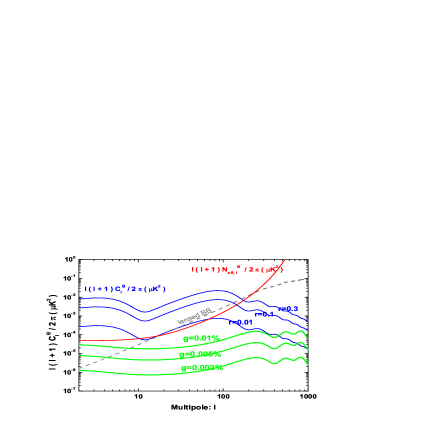
Figure 10: The contribution of differential gain to the $B$-polarization, comparing with the signal of $C_{\ell}^{B}$ for different $r$, the noise of CMBPol mission, and the lensed $B$-polarization. Left panel is for EPIC-2m, and the right panel is for EPIC-LC.

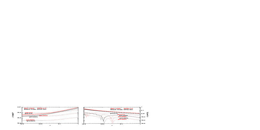
Figure 11: The values of ${\delta}r$ (left panel) and $\delta n_{t}$ (right panel) from the differential gain for different tensor-to-scalar ratio $r$. For the comparison, we plot the corresponding $\Delta r$ and $\Delta n_{t}$ in solid lines in the panels.

Let us separately investigate the five systematical effects. Fig. 10 shows $C_{\ell}^{B}({\rm sys})$ for different values of the parameter $g=0.002\%$, $0.005\%$ and $0.01\%$. In all these figures, $f_{1}=2\pi$ is used as the worst case. The values of $\ell(\ell+1)C_{\ell}^{B}({\rm sys})$ only weekly depends on the multipole $\ell$. As long as $r>0.01$, we find $C_{\ell}^{B}({\rm sys})$ are all smaller than those of the signals $C_{\ell}^{B}$ or the noises $N_{{\rm eff},\ell}^{B}$ in the range $\ell<200$. In Fig. 11, we plot the values of biases $\delta r$ and $\delta n_{t}$ induced by the differential gains. We find that the values of $\delta r$ and $\delta n_{t}$ strongly depends on the value of the parameter $g$. A larger $g$ follows a larger bias. However, the uncertainties $\Delta r$ and $\Delta n_{t}$ are nearly independent of $g$ unless the value of $g$ is too large. We also find that, given the parameter $g$ the value of the ratio $\delta r/\Delta r$ also strongly depend on the tensor-to-scalar ratio $r$. For example, the EPIC-2m experiment with $g=0.01\%$, $\delta r$ is larger than $\Delta r$ when $r<0.04$, the bias is very obvious. However when $r>0.04$, we have $\delta r<\Delta r$, the bias is smaller than the uncertainty.

Similar to the previous work dea , we can define the critical value $g_{c}$, which is the largest value of $g$ as long as the the condition $\delta r/\Delta r<0.1$ is satisfied. In Table 4, we list the critical values of $g_{c}$ for EPIC-2m and EPIC-LC, where $r=0.001$, $0.01$ and $r=0.1$ are considered. Since Fig. 11 shows that for a given $g$ value, both $\Delta r$ and $\delta r$ increase with the increasing of $r$. So the tendency of the critical $g_{c}$ for different input $r$ is not trivial. After analysis, we find that for the assumed $g$ value, with the increasing of $r$, if the increasing of $\Delta r$ is more rapid than that of $\delta r$, thus the case with larger $r$ corresponds to a larger $g_{c}$. This is clearly shown in Table 4. On the other hand, if the increasing of $\delta r$ is more rapid than that of $\Delta r$, thus the case with larger $r$ corresponds to a smaller $g_{c}$. Similar discussion is also applied to the $n_{t}$ case, as well as the cases for the other four systematics contaminations. From Table 4, we find the severest constraints are obtained from the requirement of the small $r$ case. The requirement for EPIC-2m is quite close to that of EPIC-LC.

Let us discuss the effect of beam gain on the determination of spectral index $n_{t}$. From Eq. (33), we find that the bias $e_{\ell}^{Y}$ in the lower multipole range $\ell<\ell_{t}^{*}$ contributes a negative $\delta n_{t}$, and the bias $e_{\ell}^{Y}$ in the high multipole range $\ell>\ell_{t}^{*}$ contributes a positive $\delta n_{t}$. These two components are cancelled by each other and total bias $\delta n_{t}$ is expected to be very small, which is clearly shown in Fig. 11 (right panel). Comparing with the bias of $r$, the bias $\delta n_{t}$ is much smaller than that of $\Delta n_{t}$. So the constraint on $g$ obtained from the requirement of the $n_{t}$ is much larger than that from the parameter $r$.

Now, let us turn to the effect of the differential monopole effect. From the formulae in Table 3 we know the power spectra generated by differential monopole effect strongly depend on the beam size. Larger beam size follows the larger power spectra $C_{{\rm sys},\ell}^{Y}$. This can be seen clearly in Fig. 12. Given $\mu=0.1\%$, the value of $C_{\ell}^{B}({\rm sys})$ is much larger in EPIC-LC than that in EPIC-2m. So in order to achieve a same value of $\delta r/\Delta r=0.1$, the requirement for EPIC-LC is much severer than that for EPIC-2m, which are clearly shown in Table 4. Fig. 13 shows that, for a given $\mu$, a larger $r$ follows a larger ratio value $\delta r/\Delta r$, which is correct for both EPIC-2m and EPIC-LC. In order to keep the tensor-to-scalar ratio in the range $r\in(0.001,0.1)$ unbiased, we should have $\mu_{c}=0.029\%$ for EPIC-2m, and $\mu_{c}=0.005\%$ for EPIC-LC, where $f_{1}=2\pi$ is adopted. we can also discuss the effect of differential monopole on the determination of spectral index $n_{t}$. From Fig. 12, we find that $C_{{\rm sys},\ell}^{Y}$ is sharply peaked at the high multipole, where $\ell>\ell_{t}^{*}$. Thus the total contribution to $\delta n_{t}$ is always positive (see Fig. 13), especially when the value of $\mu$ is not too small, the effect of differential monopole at the small scale is very important, and follows a fairly large bias for spectral index. Let us define the value of $\mu_{c}$, where $\delta n_{t}/\Delta n_{t}=0.1$ is satisfied. From Table 4 we find that the constraint on $\mu$ is a little severer from the parameter $n_{t}$ than that from the parameter $r$. This table shows that, the most severe constraint on $\mu$ is obtained from the requirement of $n_{t}$ in the case of $r=0.1$.

In Figs. 14 and 15, we show the effect of differential pointing on the determination of gravitational waves, where $f_{2}=2\pi$ is adopted. These figures show that similar with the case of differential monopole effect, the function $C_{\ell}^{B}({\rm sys})$ generated by differential pointing is also sharply peaked at the high $\ell$, which follows that the bias of the spectral index $\delta n_{t}$ is positive. Comparing the left panel with the right panel in Fig. 14, we find that for a given $\rho$, the effect of the differential pointing is more important for the EPIC-2m, due to the smaller instrumental noises. So more severe constraint on the differential pointing is followed for the EPIC-2m. In Table 4, we find that for both EPIC-2m and EPIC-LC, the most severe on $\rho$ comes from the requirement of parameter $n_{t}$ at $r=0.1$.

We have also investigated the effect of the differential quadrupole in Figs. 16 and 17. The effects are similar to those of the differential monopole. We find that EPIC-LC needs the much stricter requirement than EPIC-2m. For each experiment, the most severe constraint on the parameter ${\rm e}$ is obtained from the requirement of $n_{t}$ in the case with $r=0.1$.

At last, we shall discuss the effect of the differential rotation, and the results are shown in Figs. 18 and 19. We find that for a given $\varepsilon$, the ratios $\delta r/\Delta r$ and $\delta n_{t}/\Delta n_{t}$ only weakly depend on the tensor-to-scalar ratio. And the ratio for EPIC-2m is a little smaller than that of EPIC-LC. In order to keep the parameters $r$ and $n_{t}$ unbiased, the requirement $\varepsilon<0.09^{o}$ is needed for EPIC-2m, and $\varepsilon<0.15^{o}$ is needed for EPIC-LC.

As a conclusion, by analyzing the effects of the systematics on the determination of gravitational waves, we find that the requirement of $n_{t}$ unbiased follows the similar or even more severe constraints for the beam systematical parameters. For the effects of differential monopole, pointing and quadrupole, a larger $r$ follows a more severe constraint for the systematics. The critical values for the systematical parameters are listed in Table 4, where the bold entries denote the most severe constraint in each case. We also find that comparing with EPIC-2m, the low cost EPIC-LC experiment has a much high requirement for the systematical parameters $\mu$ and ${\rm e}$.

Table 3: The leading order contributions of the systematic effects to the CMB power spectra, assuming the underlying sky is not polarized (except for the rotation signal) keating , where $z\equiv(\ell\sigma)^{2}{\rm e}$ and $\sigma$ is mean beamwidth of the beam, which is calculated by $\sigma=\theta_{F}/\sqrt{8\ln 2}$. $c_{\theta}\equiv\cos(\theta)$, where $\theta$ is the angle between ellipse major axis of the elliptical gaussian beam and the horizontal $x$-axis of the fixed focal plane. $c_{\psi}\equiv\cos(\psi)$ and $s_{\psi}\equiv\sin(\psi)$, where $\psi$ is the angle between the axis of polarization sensitivity and the major axis of the elliptical beam. A clear show of the angles $\theta$ and $\psi$ can be found in Fig. 1 in keating . The definitions of the other parameters can be found in the text, see also keating .

Effect	Parameter	$C_{{\rm sys},\ell}^{C}$	$C_{{\rm sys},\ell}^{E}$	$C_{{\rm sys},\ell}^{B}$
Gain	$g$	0	$g^{2}f_{1}C_{\ell}^{T}$	$g^{2}f_{1}C_{\ell}^{T}$
Monopole	$\mu$	0	$4\mu^{2}(\ell\sigma)^{4}C_{\ell}^{T}f_{1}$	$4\mu^{2}(\ell\sigma)^{4}C_{\ell}^{T}f_{1}$
Pointing	$\rho$	$-c_{\theta}J_{1}^{2}(\ell\rho)C_{\ell}^{T}f_{3}$	$J_{1}^{2}(\ell\rho)C_{\ell}^{T}f_{2}$	$J_{1}^{2}(\ell\rho)C_{\ell}^{T}f_{2}$
Quadrupole	e	$-I_{0}(z)I_{1}(z)c_{\psi}C_{\ell}^{T}$	$I_{1}^{2}(z)c_{\psi}^{2}C_{\ell}^{T}$	$I_{1}^{2}(z)s_{\psi}^{2}C_{\ell}^{T}$
Rotation	$\varepsilon$	0	$4\varepsilon^{2}C_{\ell}^{B}$	$4\varepsilon^{2}C_{\ell}^{E}$

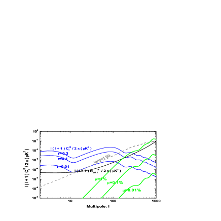
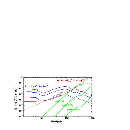
Figure 12: The contribution of monopole effect to the $B$-polarization, comparing with the signal of $C_{\ell}^{B}$ for different $r$, the noise of CMBPol mission, and the lensed $B$-polarization. Left panel is for EPIC-2m, and the right panel is for EPIC-LC.

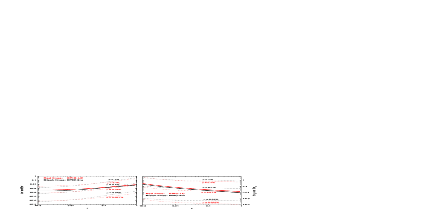
Figure 13: The values of ${\delta}r$ (left panel) and $\delta n_{t}$ (right panel) from the monopole effect for different tensor-to-scalar ratio $r$. For the comparison, we plot the corresponding $\Delta r$ and $\Delta n_{t}$ in solid lines in the panels.

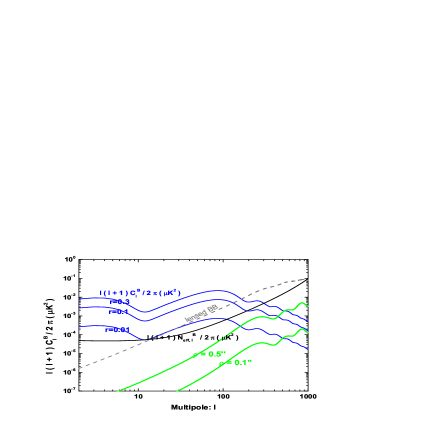
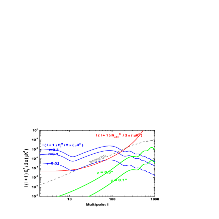
Figure 14: The contribution of differential pointing to the $B$-polarization, comparing with the signal of $C_{\ell}^{B}$ for different $r$, the noise of CMBPol mission, and the lensed $B$-polarization. Left panel is for EPIC-2m, and the right panel is for EPIC-LC.

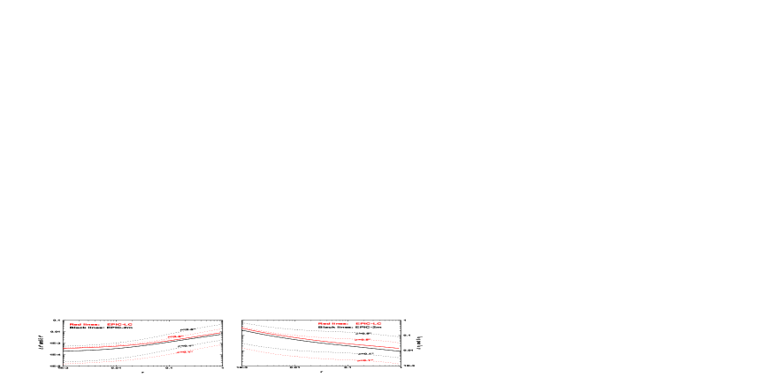
Figure 15: The values of ${\delta}r$ (left panel) and $\delta n_{t}$ (right panel) from the differential pointing for different tensor-to-scalar ratio $r$. For the comparison, we plot the corresponding $\Delta r$ and $\Delta n_{t}$ in solid lines in the panels.

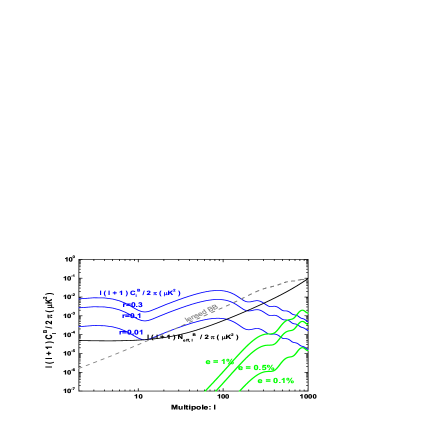
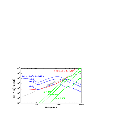
Figure 16: The contribution of quadrupole effect to the $B$-polarization, comparing with the signal of $C_{\ell}^{B}$ for different $r$, the noise of CMBPol mission, and the lensed $B$-polarization. Left panel is for EPIC-2m, and the right panel is for EPIC-LC.

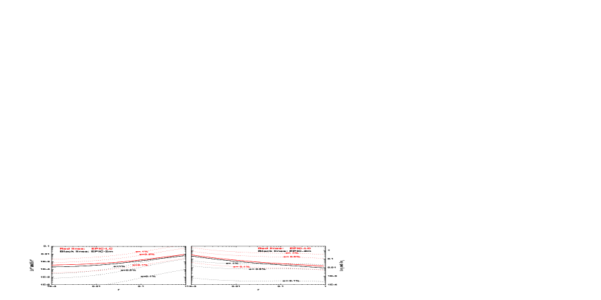
Figure 17: The values of ${\delta}r$ (left panel) and $\delta n_{t}$ (right panel) from the quadrupole effect for different tensor-to-scalar ratio $r$. For the comparison, we plot the corresponding $\Delta r$ and $\Delta n_{t}$ in solid lines in the panels.

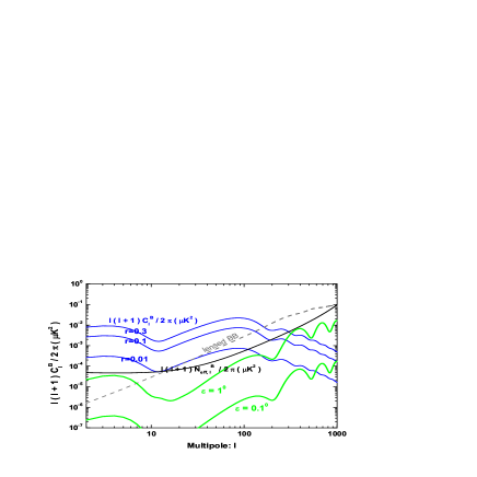
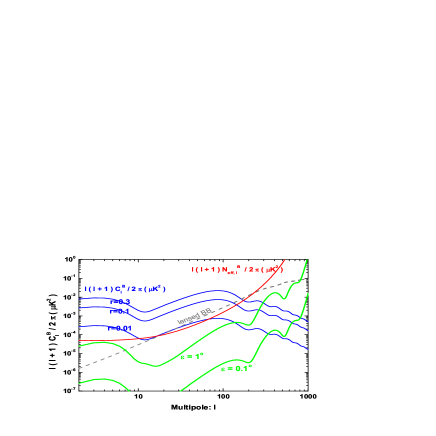
Figure 18: The contribution of differential rotation to the $B$-polarization, comparing with the signal of $C_{\ell}^{B}$ for different $r$, the noise of CMBPol mission, and the lensed $B$-polarization. Left panel is for EPIC-2m, and the right panel is for EPIC-LC.

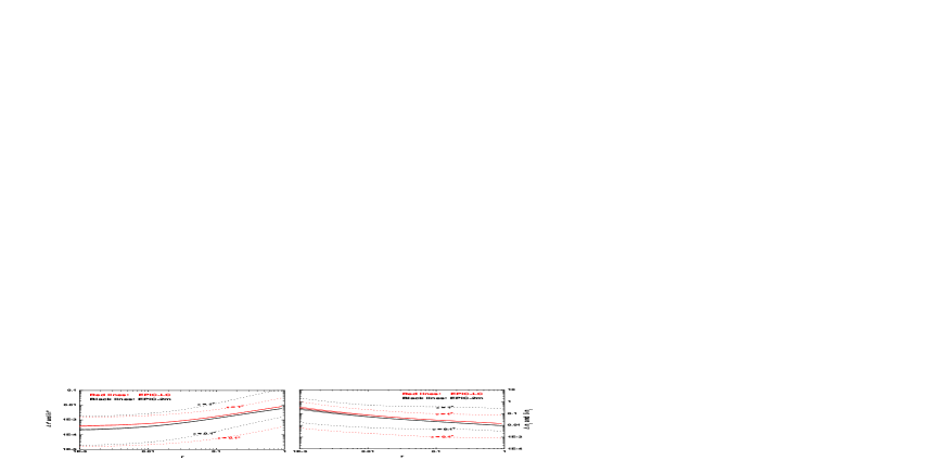
Figure 19: The values of ${\delta}r$ (left panel) and $\delta n_{t}$ (right panel) from the differential rotation for different tensor-to-scalar ratio $r$. For the comparison, we plot the corresponding $\Delta r$ and $\Delta n_{t}$ in solid lines in the panels.

Table 4: Systematics tolerance for EPIC-2m and EPIC-LC, where different nominal values of $r$ are considered. In each box, the left value is for the parameter $r$ and the right value is for the parameter $n_{t}$.

	Nominal value	$\frac{g_{c}}{1\%}\sqrt{\frac{f_{1}}{2\pi}}$	$\frac{\mu_{c}}{1\%}\sqrt{\frac{f_{1}}{2\pi}}$	$\frac{\rho_{c}}{1^{\prime\prime}}\sqrt{\frac{f_{2}}{2\pi}}$	$\frac{\rm e_{c}}{1\%}$	$\varepsilon_{c}$[deg]
	r=0.001	0.0017 & —–	0.061 & 0.042	0.096 & 0.085	0.87 & 0.59	0.11 & 0.21
EPIC-2m	r=0.01	0.0021 & —–	0.049 & 0.030	0.087 & 0.071	0.70 & 0.43	0.11 & 0.14
	r=0.1	0.0031 & —–	0.029 & 0.019	0.068 & 0.054	0.41 & 0.27	0.09 & 0.10
	r=0.001	0.0020 & —–	0.0073 & 0.0061	0.15 & 0.14	0.10 & 0.09	0.15 & 0.22
EPIC-LC	r=0.01	0.0026 & —–	0.0064 & 0.0053	0.14 & 0.13	0.09 & 0.08	0.17 & 0.19
	r=0.1	0.0039 & —–	0.0050 & 0.0040	0.13 & 0.11	0.07 & 0.06	0.18 & 0.16

VII Conclusion

The proposed CMBPol mission is the next generation of the space-based CMB experiment, which will survey the full sky and has the much smaller instrumental noises than Planck satellite. As one the most important tasks of this mission, detecting relic gravitational waves will be achieved if the tensor-to-scalar ratio $r\gtrsim 0.001$, which will provide a great opportunity to study the physics in the early Universe, especially in the inflationary stage.

In this paper, we have detailedly discussed the detection of relic gravitational waves by focusing on the constraints of the parameters $r$ and the spectral index $n_{t}$, which are always used to describe the primordial power spectrum of gravitational waves. In our discussion, we deeply investigate various contaminations for the detection, including the instrumental noises of CMBPol mission, the cosmic lensing contamination, the foreground contaminations, and the effect of various beam systematics. We found that the cosmic lensing becomes the dominant noise sources, comparing the instrumental noises for both EPIC-2m and EPIC-LC projects. Different from Planck satellite, if $r>0.01$, the detection of gravitational waves mostly depends on the observation at multipole $\ell\sim 100$, the peak of the $B$-mode polarization. However, the reionization peak at $\ell\sim 10$ still plays a crucial role for the determination of spectral index $n_{t}$. We also found that if the foreground contaminations cannot be well controlled, the reionization peak may be unobservable, which could deeply increase the uncertainty of $n_{t}$. At the same time, we have investigated the effect of various beam systematics on the detection of gravitational waves, which mainly cause a bias on the cosmological parameters. In order to keep these biases small enough, the requirements for the beam systematical parameters are quite severe, especially for the EPIC-LC mission.

References

- (1) J. Bock et al., Task force on cosmic microwave background research, [arXiv:astro-ph/0604101].
- (2) L. P. Grishchuk, Zh. Eksp. Teor. Fiz. Amplification of gravitational waves in an isotropic universe, 67, 825 (1974) [Sov. Phys. JETP 40, 409 (1975)]; Graviton creation in the early Universe, Ann. NY Acad. Sci. 302, 439 (1977); Primordial gravitons and possibility of their observation, Pis’ma Zh. Eksp. Teor. Fiz. 23, 326 (1976) [JETP Lett. 23, 293 (1976)].
- (3) L. P. Grishchuk, Discovering relic gravitational waves in cosmic microwave background radiation, Chapter in the “General Relativity and Johh Archibald Wheeler”, edited by I. Ciufolini and R. Matzner, (Springer, New York, 2010, pp. 151-199), arXiv:0707.3319.
- (4) A. A. Starobinsky, Spectrum of relict gravitational radiation and the early state of the Universe, JETP Lett. 30, 682 (1979).
- (5) V. A. Rubakov, M. Sazhin and A. Veryaskin, Graviton creation in the inflationary universe and the grand unification scale, Phys. Lett. B 115, 189 (1982).
- (6) S. Sasaki, Large scale quantum fluctuations in the inflationary universe, Prog. Theor. Phys. 76, 1036 (1986).
- (7) V. F. Mukhanov, H. A. Feldman and R. H. Brandenberger, Theory of cosmological perturbations, Phys. Rep. 215, 203 (1992).
- (8) L. P. Grishchuk, Relic gravitational waves and their detection, Lect. Notes Phys. 562, 167 (2001); Y. Zhang, Y. F. Yuan, W. Zhao and Y. T. Chen, Relic gravitational waves in the accelerating Universe, Class. Quant. Grav. 22, 1383 (2005); T. L. Smith, H. V. Peiris and A. Cooray, Deciphering inflation with gravitational waves: Cosmic microwave background polarization vs direct detection with laser interferometers, Phys. Rev. D 73, 123503 (2006); W. Zhao and Y. Zhang, Relic gravitational waves and their detection, Phys. Rev. D 74, 043503 (2006).
- (9) Y. Watanabe and E. Komatsu, Improved calculation of the primordial gravitational wave spectrum in the standard model, Phys. Rev. D 73, 123515 (2006); L. A. Boyle and P. J. Steinhardt, Probing the early universe with inflationary gravitational waves, Phys. Rev. D 77, 063504 (2008); M. Giovannini, Production and detection of relic gravitons in quintessential inflationary models, Phys. Rev. D 60, 123511 (1999), Spikes in the relic graviton background from quintessential inflation, Class. Quant. Grav. 16, 2905 (1999), Stochastic backgrounds of relic gravitons, TCDM paradigm and the stiff ages, Phys. Lett. B 668, 44 (2008), Thermal history of the plasma and high-frequency gravitons, Class. Quant. Grav. 26, 045004 (2009).
- (10) D. H. Lyth and A. Riotto, Particle physics models of inflation and the cosmological density perturbation, Phys. Rep. 314, 1 (1999).
- (11) S. Kachru et al., Towards inflation in string theory, JCAP, 0310, 013 (2003); D. Baumann and L. McAllister, A microscopic limit on gravitational waves from D-brane inflation, Phys. Rev. D 75, 123508 (2007); E. Silverstein and D. Tong, Scalar speed limits and cosmology: Acceleration from D-ceeleration, Phys. Rev. D 70, 103505 (2004); R. Kallosh and A. Liddle, Testing string theory with CMB, JCAP, 0704, 017 (2007).
- (12) A. Polnarev, Polarization and anisotropy induced in the microwave background by cosmological gravitational waves, Sov. Astron. 29, 607 (1985); D. Harari and M. Zaldarriaga, Polarization of the microwave background in inflationary cosmology, Phys. Lett. B 319, 96 (1993); L. P. Grishchuk, Cosmological perturbations of quantum-mechanical origin and anisotropy of the microwave background, Phys. Rev. Lett. 70, 2371 (1993); R. Crittenden, J. R. Bond, R. L. Davis, G. Efstathiou and P. J. Steinhardt, Imprint of gravitational waves on the cosmic microwave background, Phys. Rev. Lett. 71, 324 (1993); R. A. Frewin, A. G. Polnarev and P. Coles, Gravitational waves and the polarization of the cosmic microwave background, Mon. Not. R. Astron. Soc. 266, L21 (1994).
- (13) U. Seljak and M. Zaldarriaga, Signature of gravity waves in the polarization of the microwave background, Phys. Rev. Lett. 78, 2054 (1997); M. Kamionkowski, A. Kosowsky and A. Stebbins, A probe of primordial gravity waves and vorticity, Phys. Rev. Lett. 78, 2058 (1997).
- (14) M. Zaldarriaga and U. Seljak, All-sky analysis of polarization in the microwave background, Phys. Rev. D 55, 1830 (1997).
- (15) J. R. Pritchard and M. Kamionkowski, Cosmic microwave background fluctuations from gravitational waves: An analytic approach, Ann. Phys. (N.Y.) 318, 2 (2005); W. Zhao and Y. Zhang, Analytic approach to the CMB polarization generated by relic gravitational waves, Phys. Rev. D 74, 083006 (2006); D. Baskaran, L. P. Grishchuk and A. G. Polnarev, Imprints of relic gravitational waves in cosmic microwave background radiation, Phys. Rev. D 74, 083008 (2006); T. Y. Xia and Y. Zhang, Analytic spectra of CMB anisotropies and polarization generated by relic gravitational waves with modification due to neutrino free-streaming, Phys. Rev. D 78, 123005 (2008), Approximate analytic spectra of reionized CMB anisotropies and polarization generated by relic gravitational waves, Phys. Rev. D 79, 083002 (2009).
- (16) B. G. Keating, A. G. Polnarev, N. J. Miller and D. Baskaran, The polarization of the cosmic microwave background due to primordial gravitational waves, Int. J. Mod. Phys. A 21, 2459 (2006); R. Flauger and S. Weinberg, Tensor microwave background fluctuations for large multipole order, Phys. Rev. D 75, 123505 (2007); Y. Zhang, W. Zhao, X. Z. Er, H. X. Miao and T. Y. Xia, Relic gravitational waves and CMB polarization in the accelerating Universe, Int. J. Mod. Phys. D 17, 1105 (2008).
- (17) A. G. Polnarev, N. J. Miller and B. G. Keating, CMB temperature polarization correlation and primordial gravitational waves , Mon. Not. R. Astron. Soc. 386, 1053 (2008); N. J. Miller and B. G. Keating and A. G. Polnarev, CMB temperature polarization correlation and primordial gravitational waves II: Wiener filtering and tests based on Monte Carlo simulations, arXiv:0710.3651.
- (18) W. Zhao, D. Baskaran and L. P. Grishchuk, On the road to discovery of relic gravitational waves: The TE and BB correlations in the cosmic microwave background radiation, Phys. Rev. D 79, 023002 (2009).
- (19) E. Komastu et al., Seven-Year Wilkinson Microwave Anisotropy Probe (WMAP) observations: Cosmological interpretation, arXiv:1001.4538.
- (20) W. Zhao, D. Baskaran and L. P. Grishchuk, On the road to discovery of relic gravitational waves: The TE and BB correlations in the cosmic microwave background radiation, Phys. Rev. D 79, 023002 (2009), Stable indications of relic gravitational waves in Wilkinson Microwave Anisotropy Probe data and forecasts for the Planck mission, Phys. Rev. D 80, 083005 (2009), Relic gravitational waves in light of the 7-year Wilkinson Microwave Anisotropy Probe data and improved prospects for the Planck mission, Phys. Rev. D 82, 043003 (2010); W. Zhao and L. P. Grishchuk, Relic gravitational waves: Latest revisions and preparations for new data, Phys. Rev. D 82, 123008 (2010).
- (21) Planck Collaboration, The science programme of Planck, [arXiv:astro-ph/0604069].
- (22) W. Zhao, Detecting relic gravitational waves in the CMB: Comparison of different methods, Phys. Rev. D 79, 063003 (2009).
- (23) Y. Z. Ma, W. Zhao and M. L. Brown, Constraints on standard and non-standard early Universe models from CMB B-mode polarization, JCAP, 1010, 007 (2010).
- (24) W. Zhao and D. Baskaran, Detecting relic gravitational waves in the CMB: Optimal parameters and their constraints, Phys. Rev. D 79, 083003 (2009).
- (25) B. G. Keating et al., BICEP: A large angular scale CMB polarimeter, in Polarimetry in Astronomy, edited by Silvano Fineschi, Proceedings of the SPIE, 4843 (2003); C. Pryke et al., QUaD Collaboration, Second and third season QUaD CMB temperature and polarization power spectra, Astrophys. J. 692, 1247 (2009); A. C. Taylor, Clover Collaboration, Clover - A B-mode polarization experiment, New Astron. Rev. 50, 993 (2006); J. Errard, The new generation CMB B-mode polarization experiment: POLARBEAR, arXiv:1011.0763; http://bolo.berkeley.edu/polarbear/index.html; D. Samtleben, Measuring the cosmic microwave background radiation (CMBR) polarization with QUIET, arXiv:0802.2657; http://quiet.uchicago.edu/; J.A. Rubino-Martin et al., The Quijote CMB Experiment, arXiv:0810.3141; http://www.iac.es/project/cmb/quijote/; http://pole.uchicago.edu/; http://wwwphy.princeton.edu/act/; The QUBIC Collaboration, QUBIC: The QU Bolometric Interferometer for Cosmology, arXiv:1010.0645.
- (26) http://groups.physics.umn.edu/cosmology/ebex/index.html; A. Kogut, et al., PAPPA: Primordial Anisotropy Polarization Pathfinder Array, New Astron. Rev. 50, 1009 (2006); B.P. Crill, et al., SPIDER: A balloon-borne large-scale CMB polarimeter , arXiv:0807.1548.
- (27) W. Zhao and W. Zhang, Detecting relic gravitational waves in the CMB: Comparison of Planck and ground-based experiments, Phys. Lett. B 677, 16 (2009).
- (28) D. Baumann et al., CMBPol mission concept study: Probing inflation with CMB polarization, arXiv:0811.3919.
- (29) B-Pol Collaboration, B-Pol: Detecting primordial gravitational waves generated during inflation, Exper. Astron. 23, 5 (2009); http://www.b-pol.org/index.php.
- (30) http://cmbpol.kek.jp/litebird/.
- (31) L. P. Grishchuk and M. Solokhin, Spectra of relic gravitons and the early history of the Hubble parameter, Phys. Rev. D 43, 2566 (1991); A. Kosowsky and M. S. Turner, CBR anisotropy and the running of the scalar spectral index, Phys. Rev. D 52, 1739 (1995).
- (32) E. D. Stewart and D. H. Lyth, A more accurate analytic calculation of the spectrum of cosmological perturbations produced during inflation, Phys. Lett. B 302, 171 (1993).
- (33) H. V. Peiris et al., First Year Wilkinson Microwave Anisotropy Probe (WMAP) observations: Implications for inflation, Astrophys. J. Suppl. Ser. 148, 213 (2003).
- (34) E. Komatsu et al., Five-Year Wilkinson Microwave Anisotropy Probe (WMAP) observations: Cosmological interpretation, Astrophys. J. Suppl. Ser. 180, 330 (2009).
- (35) A. Lewis, A. Challinor and A. Lasenby, Efficient computation of CMB anisotropies in closed FRW models, Astrophys. J. 538, 473 (2000); http://camb.info/.
- (36) M. J. Mortonson and W. Hu, Model-independent constraints on reionization from large-scale CMB polarization, Astrophys. J. 672, 737 (2008); M. J. Mortonson and W. Hu, Impact of reionization on CMB polarization tests of slow-roll inflation, Phys. Rev. D 77, 043506 (2008); M. J. Mortonson and W. Hu, Reionization constraints from five-year WMAP data, Astrophys. J. 686, L53 (2008).
- (37) S. Hamimeche and A. Lewis, Likelihood analysis of CMB temperature and polarization power spectra, Phys. Rev. D 77, 103013 (2008).
- (38) W. J. Percival and M. L. Brown, Likelihood methods for the combined analysis of CMB temperature and polarisation power spectra, Mon. Not. R. Astron. Soc. 372, 1104 (2006); H. K. Eriksen and I. K. Wehus, Marginal distributions for cosmic variance limited CMB polarization data, Astrophys. J. Suppl. Ser. 180, 30 (2009).
- (39) A. Lewis and S. L. Bridle, Cosmological parameters from CMB and other data: A Monte Carlo approach, Phys. Rev. D 66, 103511 (2002).
- (40) A. Lewis, Harmonic E/B decomposition for CMB polarization maps, Phys. Rev. D 68, 083509 (2003); A. Lewis, A. Challinor and N. Turok, Analysis of CMB polarization on an incomplete sky, Phys. Rev. D 65, 023505 (2001); E. F. Bunn, M. Zaldarriaga, M. Tegmark and A. de Oliveira-Costa, E/B decomposition of finite pixelized CMB maps, Phys. Rev. D 67, 023501 (2003); E. F. Bunn, E/B mode mixing, arXiv:0811.0111; Efficient decomposition of cosmic microwave background polarization maps into pure E, pure B, and ambiguous components, arXiv:1008.0827.
- (41) K. M. Smith, Pseudo-Cl estimators which do not mix E and B modes , Phys. Rev. D 74, 083002 (2006); J. Grain, M. Tristram and R. Stompor, Polarized CMB power spectrum estimation using the pure pseudo-cross-spectrum approach, Phys. Rev. D 79, 123515 (2009); K. M. Smith and M. Zaldarriaga, General solution to the E-B mixing problem, Phys. Rev. D 76, 043001 (2007).
- (42) W. Zhao and D. Baskaran, Separating E and B types of polarization on an incomplete sky, Phys. Rev. D 82, 023001 (2010); J. Kim and P. Naselsky, CMB E/B decomposition of incomplete sky: a pixel space approach, Astronomy and Astrophysics 519, A104 (2010); J. Kim, How to make clean separation of CMB E and B mode from incomplete sky data, arXiv:1010.2636.
- (43) J. Bock et al., Study of the Experimental probe of Inflationary Cosmology (EPIC)-Intemediate mission for NASA’s Einstein Inflation Probe, arXiv:0906.1188.
- (44) M. Zaldarriaga and U. Seljak, Gravitational lensing effect on cosmic microwave background polarization, Phys. Rev. D 58, 023003 (1998).
- (45) W. Hu and T. Okamoto, Mass reconstruction with CMB polarization, Astrophys. J. 574, 566 (2002); T. Okamoto and W. Hu, CMB lensing reconstruction on the full sky, Phys. Rev. D 67, 083002 (2003).
- (46) C. M. Hirata and U. Seljak, Reconstruction of lensing from the cosmic microwave background polarization, Phys. Rev. D 68, 083002 (2003); U. Seljak and C. M. Hirata, Gravitational lensing as a contaminant of the gravity wave signal in the CMB, Phys. Rev. D 69, 043005 (2004).
- (47) A. Lewis and A. Challinor, Weak gravitational lensing of the CMB, Phys. Rep. 429, 1 (2006).
- (48) K. M. Smith et al., CMBPol mission concept study: Gravitational lensing, arXiv:0811.3916.
- (49) L. Knox and Y. S. Song, Limit on the detectability of the energy scale of inflation, Phys. Rev. Lett. 89, 011303 (2002); M. Kesden, A. Cooray and M. Kamionkowski, Separation of gravitational-wave and cosmic-shear contributions to cosmic microwave background polarization, Phys. Rev. Lett. 89, 011304 (2002).
- (50) C. L. Bennett et al., First Year Wilkinson Microwave Anisotropy Probe (WMAP) observations: Foreground emission, Astrophys. J. Suppl. Ser. 148, 97 (2003).
- (51) J. Dunkely et al., CMBPol mission concept study: Prospects for polarized foreground removal, arXiv:0811.3915.
- (52) L. Verde, H. Peiris and R. Jimenez, Considerations in optimizing CMB polarization experiments to constrain inflationary physics, JCAP, 0601, 019 (2006).
- (53) L. Page et al., Three Year Wilkinson Microwave Anisotropy Probe (WMAP) Observations: Polarization Analysis, Astrophys. J. Suppl. Ser. 170, 335 (2007).
- (54) E. M. Finkbeiner et al., Extrapolation of galactic dust emission at 100 microns to CMBR frequencies using FIRAS, Astrophys. J. 624, 10 (2001).
- (55) J. Kim, P. Naselsky and P. R. Christensen, CMB polarization map derived from the WMAP 5 year data through the harmonic internal linear combination method, Phys. Rev. D 79, 023003 (2009); G. Efstathiou, S. Gratton and F. Paci, Impact of galactic polarized emission on B-mode detection at low multipoles, Mon. Not. Roy. Astron. Soc. 397, 1355 (2009).
- (56) W. Zhao and Q. G. Huang, Testing inflationary consistency relations by the potential CMB observations, arXiv:1101.3163.
- (57) W. Hu, M. M. Hedman and M. Zaldarriaga, Benchmark parameters for CMB polarization experiments, Phys. Rev. D 67, 043004 (2003).
- (58) M. Su, A. P. S. Yadav and M. Zaldarriaga, Impact of instrumental systematic contamination on the lensing mass reconstruction using the CMB polarization, Phys. Rev. D 79, 123002 (2009); M. Su, A. P. S. Yadav, M. Shimon and B. G. Keating, Impact of instrumental systematics on the CMB bispectrum, arXiv:1010.1957.
- (59) M. Shimon, B. Keating, N. Ponthieu and E. Hivon, CMB polarization systematics due to beam asymmetry: Impact on inflationary science, Phys. Rev. D 77, 083003 (2008); N. J. Miller, M. Shimon and B. G. Keating, CMB beam systematics: Impact on lensing parameter estimation, Phys. Rev. D 79, 063008 (2009); CMB polarization systematics due to beam asymmetry: Impact on cosmological birefringence, Phys. Rev. D 79, 103002 (2009).
- (60) D. O’Dea, A. Challinor and B. R. Johnson, Systematic errors in cosmic microwave background polarization measurements, Mon. Not. Roy. Astron. Soc. 376, 1767 (2007).