Two real parton contributions to non-singlet kernels for exclusive QCD DGLAP evolution

Abstract

Results for the two real parton differential distributions needed for implementing a next-to-leading order (NLO) parton shower Monte Carlo are presented. They are also integrated over the phase space in order to provide solid numerical control of the MC codes and for the discussion of the differences between the standard $\overline{MS}$ factorization and Monte Carlo implementation at the level of inclusive NLO evolution kernels. Presented results cover the class of non-singlet diagrams entering into NLO kernels. The classic work of Curci-Furmanski-Pertonzio was used as a guide in the calculations.

1 Introduction

With the start of the operation of the Large Hadron Collider (LHC) in CERN and the progress in the analysis of growing data samples for many scattering processes, mastering the precise evaluation of strong interactions effects within perturbative Quantum Chromodynamics (QCD) Gross:1973ju ; Gross:1974cs ; Georgi:1951sr will become quickly more and more important. QCD is a well established theory – testing the validity of QCD is not an open issue any more. Its principal role in the LHC data analysis will be providing precise predictions for rates and distributions of quarks, gluons and hopefully other newly found particles carrying colour charge, being part of either signal process or background.

The most important theoretical tools in perturbative QCD (pQCD) calculations, apart from Feynman diagrams, renormalization, etc. are the so called factorization theorems, see for instance Ellis:1978ty ; Collins:1984kg ; Bodwin:1984hc , which allow to describe any scattering process with a single large mass or transverse momentum scale $\mu_{F}$ (enforcing short distance interaction), in terms of the on-shell hard process matrix element (ME) squared and convoluted with the ladder parts. The hard process is calculated up to a fixed perturbative order. The ladder parts are defined for each colored energetic parton entering (exiting) the hard process. The initial state ladders are conveniently encapsulated in the inclusive parton distribution functions, PDFs.

The logarithmic dependence of the parton distribution functions (PDFs) on the large scale $\mu_{F}$ is described as a DGLAP DGLAP evolution of the PDFs. This evolution was studied for the inclusive PDFs up to NLO level in the early 80’s, see refs. Floratos:1978ny ; Curci:1980uw , and was recently established at the NNLO level Moch:2004pa ; Vogt:2004mw .

Instead of being encapsulated in the inclusive PDF, the multi-parton emission process of the initial state ladder, can be modelled using direct stochastic simulation in terms of four-momenta and other quantum numbers, within the Monte Carlo (MC) parton shower. Here, the baseline works have been done in mid-80’s, see refs. Sjostrand:1985xi ; Webber:1984if , where the leading order (LO) ladder was implemented in parton shower MC (PSMC) programs. Standard LO level PSMCs implement also the process of hadronization of the light quarks and gluons into hadrons and play an important role in the software for all collider experiments because of that.

Fulfilling the challenging requirements on the quality and precision of the pQCD calculations, needed for the experimental data analysis at the LHC, enforces for the first time an urgent solution of the problem of upgrading exclusive PSMC to the complete NLO level, the same level, which was reached for inclusive PDFs two decades ago. This task is highly nontrivial mainly because the classic factorization theorems Ellis:1978ty ; Collins:1984kg ; Bodwin:1984hc were never designed for the exclusive MC implementation, but rather for defining inclusive PDFs and performing fixed order calculations for the hard process, convoluted with these PDFs.

Let us comment briefly on the longer term physics impact of the present work. Remembering that QCD is not any more a new theory, the main impact of this work will be the improvement of calculations of QCD effects, for hadron collider experiments like LHC, with the aim of improving chances of discovering directly or indirectly New Physics and/or better measurement of the Electroweak Standard Model parameters, especially when high statistics, high precision data are accumulated.

More precisely, this work elaborates on pQCD effects in the initial state, which from the perspective of the LHC experiments influence mainly: (A) overall normalization of the hard processes through parton luminosities, (B) distributions of transverse momenta ($k_{T}$) of incoming partons deforming many other important distributions in any hard process, including searches for supersymmetry, etc., (C) and provide one or more jets accompanying hard process.

The longstanding problem in the data analysis is that the above three classes of important QCD effects are addressed by three separate theoretical pQCD calculational tools, based on different incompatible perturbative techniques: (A) strictly collinear NLO PDFs DGLAP , (B) semi-inclusive schemes of infinite order soft gluon $k_{T}$ resummation Collins:1984kg ; Kulesza:1999sg ; Kulesza:2002rh or, alternatively, LO parton shower Monte Carlos Sjostrand:1985xi ; Marchesini:1988cf (C) finite order NLO (NNLO) calculations Altarelli:1979ub ; Anastasiou:2003ds sometimes combined with a LO parton shower MC Frixione:2002ik or collinear PDFs.

In the analysis of experimental data combining these (and other) techniques is not only inconvenient, but also is a serious source of irreducible theoretical (and experimental) uncertainties. This old and well known problem becomes more severe with the increasing precision of the collider data, and will inevitably plague high statistics, high precision LHC data. The ultimate aim of the present work is to provide a basis for designing a single Monte Carlo program addressing all three classes of the above pQCD effects at once, within the same consistent pQCD theoretical framework. However, for this to be realized one has to start with solving one basic difficult problem – the upgrade of the initial state parton shower MC to at least the same level as standard PDFs, that is to the NLO level, in the fully exclusive manner. The present work provides essential building blocks (exclusive kernels) for this critical extension of the parton shower, and analyzes factorization scheme differences with respect to the standard CFP $\overline{MS}$ scheme. While this work focuses on the implementation of NLO corrections to the initial state ladder parts (parton showers), the hard process part at NLO within the same scheme is discussed in ref. Jadach:2011cr .

The critical problems to be solved on the way to NLO PSMC are the following:

1. Violation of four momentum conservation. In the standard collinear factorization four momentum conservation is broken both between the hard process and the ladder as well as between the ladder segments (2PI kernels). The source of this non-conservation in the standard collinear factorization is the introduction of the projection operators, $P_{kin}$ in ref. Ellis:1978ty , operator $\mathbbm{P}$ in ref. Curci:1980uw , or operator $Z$ in ref. Collins:1998rz . These operators are absent in the first step of the separation of the collinear singularities into the ladder parts – they are introduced later on in order to (i) conveniently isolate the lightcone variable integration out of the phase space for analytical integration and (ii) facilitate the order-by-order pQCD calculations separately for the hard process ME and the ladder elements (kernels). This non-conservation happens in the transverse momenta, which are anyway treated inclusively (integrated over), hence this bad feature of collinear factorization goes almost unnoticed. In the traditional LO PSMCs the above non-conservation is repaired “by hand” Sjostrand:1985xi ; Webber:1984if , but in such a way that the NLO effects induced by this reparation are analytically almost uncontrollable. This is not a problem, unless one attempts to complete NLO in the ladder, or to combine an NLO hard process ME with a LO PSMC Frixione:2002ik . A systematic solution of the above problem must involve replacing the projection operator $P_{kin}$ by a more sophisticated operation involving a special parametrization of the entire phase space for the hard process and the ladders. An explicit example of such a solution for the $W/Z$ production process (Drell-Yan process) can be found in ref. Jadach:2011cr .

2. Separation of singularities before phase-space integrations. In the collinear factorization, separation of the LO singular contributions in the form of the leading logarithm $\ln\frac{Q^{2}}{m^{2}}$ or $\frac{1}{\varepsilon}$ poles of dimensional regularization can be done only after the phase space integration. In order to construct an efficient Monte Carlo algorithm this separation has to be done at the very beginning, at the integrand level, before the phase space integration. This requires going beyond the inherently inclusive approach of collinear factorization. The effort of getting the NLO prediction for the semi-inclusive distribution in the phase space of the hard process (like $k_{T}$ and rapidity distributions in $W/Z$ production) started already quite early, see for instance Altarelli:1979ub ; Altarelli:1984pt . More recently, Monte Carlo tools combining NLO ME for the hard process with the LO PSMC were developed in Frixione:2002ik and Nason:2004rx . Studies on redefining PDFs in a partly exclusive form beyond LO (unintegrated PDFs) Collins:1984kg , or in exclusive form (fully unintegrated PDFs) Collins:2007ph are also pursued.

3. Negative “probability distributions”. The NLO corrections in collinear factorization are negative in some regions of phase space and therefore cannot be generated directly in the Monte Carlo, if we insist on the realistic simulation using positive-weight MC events. The reasons for non-positiveness of the NLO corrections is well understood. For instance, in the physical gauge positive squares of the Feynman diagrams are typically more divergent and form the LO approximation, while non-positive interferences are collected in NLO corrections. The use of kinematic projection operators in factorization and related subtractions are another sources. The factorization procedure collects all these non-positive corrections into separate objects and the integration over the phase space is done for each of them separately. Consequently, part of the factorization procedure has to be reversed in order to recombine non-positive NLO distributions with the positive LO distributions, before the MC algorithm is designed. The above defactorization procedure has to be outlined. An example proposal relying on Bose-Einstein symmetrization was formulated in ref. Jadach:2010ew and an even more promissing one is described in ref. Jadach:2010aa (similar to that in ref. yfs:1961 ).

4. Lack of the published exclusive NLO distributions. We have not found exclusive NLO distributions forming the NLO corrections in the ladder part in literature – all published results in the context of the NLO calculations of kernels for evolution of PDFs are integrated over the phase space. The main objective of this paper is to provide such distributions for the non-singlet case.

5. Inclusive treatment of multigluon soft limit. One of the critical issues in any type of collinear factorization is the behavior of many-gluon distributions in the soft limit. In the inclusive approach it is enough to know that the cancellations between real and virtual soft contributions allow us in principle to neglect entire classes of diagrams and/or divergent contributions – they sum up to zero. In the exclusive MC approach these contributions/singularities, instead of being dropped out, have to be modelled precisely to infinite order. The above soft gluon behavior is rather well known, albeit more complicated in QCD than in QED due to the (non-abelian) triple gluon vertex – the eikonal limit and angular ordering are known to govern it khoze-book . In ref. Slawinska:2009gn a detailed analysis of the soft limit for the $C_{F}^{2}$ and $C_{F}C_{A}$ contributions for non-singlet evolution kernels was performed and the well known angular ordering was exposed, both numerically and analytically, for the first time using exact double gluon distributions presented explicitly.

6. Inappropriateness of $\overline{MS}$ factorization scheme. The issue of factorization scheme dependence has to be revisited and one has to decide about the best factorization scheme (FS) for the PSMC implementation. It should not be taken for granted that it will be the $\overline{MS}$ scheme, which is presently the “industry standard” for the inclusive PDFs and in pQCD calculations for the hard process. In the view of the above the following question emerges: Can one stay strictly within the $\overline{MS}$ scheme for the MC implementation of the NLO ladders combined with the NLO hard process ME? In the present work we will addres this question partly, for the MC modelling of the ladder part. It is studied for the hard process ME in ref. Jadach:2011cr . Let us indicate that our answer will be negative: FS of the NLO MC has to differ from $\overline{MS}$ scheme for several reasons. Some of them will be discussed in detail in this paper. The key element defining FS are the so-called soft collinear counterterms. In MC we choose them to be identical with the distribution used in the LO MC, e.g. the LO level PSMC is constructed by means of iterating soft collinear counterterms. This choice on one hand will simplify NLO corrections in the MC, but it will also cause departure from the $\overline{MS}$ FS. The second source of discrepancy will be the fact that in the MC, the factorization scale will be identical to a well defined kinematic variable $Q_{F}$ of the LO MC, replacing the formal parameter $\mu_{F}$ of the $\overline{MS}$ FS. The logarithm of $Q_{F}$ is then used in the MC as an ordered evolution time variable. $Q_{F}$ will typically be maximum transverse momentum, maximum angle, or virtuality of the emitted particles. For the gluonstrahlung, the choice of the maximum transverse momentum results in the MC FS very close to $\overline{MS}$ FS. However, the soft gluon eikonal limit for contributions like gluon pair production or quark-gluon transitions, dictates the use of the variable related to the maximum angle (rapidity) as a factorization scale variable in the MC. Third reason is the presence in the $\overline{MS}$ FS of certain artifacts of dimensional regularization which cannot be implemented in the MC in four dimensions.

7. Constrained evolution. Constrains on the momenta and other quantum numbers imposed by the hard process on the initial state parton shower (ladder), especially important in the presence of the narrow resonances, must be taken into account by the PSMC. The clever and powerfull MC technique of backward evolution of ref. Sjostrand:1985xi is good for the LO PSMC, but for the NLO case one may need something more sophisticated. The dependence of the ladder part (PDF) on the factorization scale is described in pQCD by the integro-differential DGLAP DGLAP evolution equation. Its solution has the form of a time ordered (T.O.) exponential with the ordering in the logarithm of the factorization scale. This T.O. exponential can also be obtained directly from the ladder Feynman diagrams. In the Monte Carlo T.O. exponential is conveniently modelled using a Markovian MC algorithm. However, a Markovian MC algorithm would be highly inefficient for modelling the initial state radiation (ISR) ladder, when hard process selects very narrow range of energies and flavors of the partons incoming into hard process (with narrow W/Z resonances). Here, the backward evolution MC algorithm is a standard solution Sjostrand:1985xi – used in all standard LO PSMCs. It is to be seen whether backward evolution MC is upgradable to NLO PSMC. In the meantime, the constrained MC algorithm of refs. Jadach:2005bf ; Jadach:2005yq offers an interesting alternative. While the backward evolution MC needs pretabulated solutions (PDFs) of the evolution equations, which have to be prepared beforehand using non-MC auxiliary codes, the constrained MC performs evolution on its own.

In this article we mainly addres point 4 in the above list of problems. However also point 6 is discussed in some detail.

Let us now establish precise terminology concerning diagrams and phase space integration. We will elaborate on the diagrams contributing to non-singlet evolution kernels at the NLO level.

Generally, in the calculation of the exclusive/inclusive evolution kernels in this work we will take paper of Curci Furmanski and Petronzio Curci:1980uw (CFP) as the starting point and as the reference in all NLO calculations. For the non-singlet part of the QCD DGLAP evolution we will calculate (or recalculate) both the standard inclusive NLO kernels and the new exclusive (unintegrated) ones, which are needed for constructing NLO PSMC. This work prepares building blocks for NLO PSMC, whereas the actual MC algorithm and all issues related to the factorization scheme used in NLO PSMC will be discussed in a separate paper Jadach:2011cr .

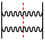
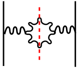
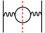
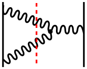
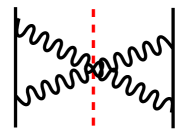
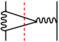
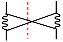
Figure 1: Real contributions to NLO non-singlet DGLAP kernel.

Our main object of interest in the present work are the diagrams depicted in Fig. 1, with two emitted on-shell quarks and/or gluons, that is diagrams with two cut lines. We will call them 2-real, or shortly 2R, contributions. The other diagrams with 1-real and 1-virtual, nicknamed 1V1R, will be also partly considered. Diagrams with 2 virtual (2V) will not be discussed, because they will be treated in the same way as in CFP (deduced from the baryon number conservation rule, which we keep in the Monte Carlo by construction).

The NLO 2PI diagrams feature amplitude-squares, depicted in the upper row in Fig. 1: double gluon emission 1, gluon pair production 1 and fermion pair production 1 as well as interferences, displayed in the lower row in Fig. 1. Interference diagrams enter into the MC kernels for the first time at NLO and their correct incorporation in the MC requires more care. They can potentially make negative contributions to the kernel, spoiling the MC weight. It turns out that the interference diagrams have different statuses in the MC, in the following we explain the reasons for it.

Let us make a simple observation that interferences 1 and 1 together with squares 1 and 1 form the full amplitude square

$$\Bigg{|}~{}~{}\raisebox{-11.0pt}{\includegraphics[height=31.29802pt]{2g_sum.pdf}}\Bigg{|}^{2}.$$

Positiveness of this amplitude square will cause the MC weight introducing these two interferences to be positive. Both interferences 1 and 1 can be implemented in the MC in the 2R group of diagrams.

The interference diagram 1 originates from the following amplitude-squared

$$\Bigg{|}~{}~{}\raisebox{-11.0pt}{\includegraphics[height=31.29802pt]{sumqq.pdf}}\Bigg{|}^{2},$$

where $q\bar{q}$ pair production 1 is already included in the non-singlet class, while $q\bar{q}$ transitions amplitude (squared) belongs to the singlet kernel. Apparently, diagram 1 corrects quark-gluon transitions absent in non-singlet kernel and must be included in the MC together with the singlet contributions.

Similarly, the diagram 1 is the interference part in the amplitude square

$$\Bigg{|}~{}~{}\raisebox{-11.0pt}{\includegraphics[height=31.29802pt]{sum3.pdf}}\Bigg{|}^{2},$$

where both amplitudes representing $q\bar{q}$ transitions essentially belong to the singlet NLO kernel.

In the case of both interferences related to quark-gluon transitions the MC weight is not protected by the Schwartz inequality due to the absence of amplitude squares in the non-singlet kernels. The above problem will naturally disappear when singlet diagrams are included in the game, and we need some temporary fix, while staying in the non-singlet class. In order to keep the fermion number conservation we keep these contributions in the kernel, but add them to the 1R1V class and treat inclusively. In the following such a combination of the 1R1V and integrated subclass of 2R interferences we will call collectively unresolved contribution.

Another important point concerns internal singularities of Feynman diagrams. They are present in graphs of Fig. 1, 1 and 1. The double bremsstrahlung diagram Fig. 1 does not enter into NLO kernel as a whole but only what remains after subtracting soft collinear counterterm of the CFP factorization. On the other hand, diagram of Fig. 1 features internal collinear singularity cancelled by the corresponding virtual (gluon self-energy) diagram. These diagrams may enter into the unresolved part in the MC, or may be modelled in an exclusive manner. In the latter case diagram 1 requires the construction of a dedicated soft-collinear counterterm which encapsulates the above internal singularities and is instrumental in the MC construction. Such a counterterm will be defined in Section 3.6. Diagram 1 can be also modelled in an exclusive way and also needs a dedicated counterterm, see Section 4.3.

Before that, Section 2 presents an overview of calculations illustrated by the example of the LO kernel. Notation and methodology of extracting kernels will be introduced using this simple example. The integration procedure for NLO kernels is reviewed in Sections 3 and 4. The contributions from each appropriate Feynman diagram in the axial gauge are calculated in integrated and unintegrated form needed for the MC. Analytical integration for control will also be done. Discussion of the collinear and soft singularity structure will have the highest priority.

Sections 3 and 4 summarize results of analytical integrations. In contrast to the results presented in Curci:1980uw , 2R contributions will be shown separately instead of the sum of 2R and 1R1V. Section 5 provides final discussions and conclusions.

2 Leading order example

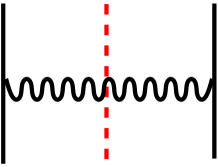
Figure 2: Born level diagram.

Using the LO diagram of Fig. 2 we are going to introduce some basic notation, which will also be useful in the NLO calculations. In addition we will show correspondence between elements of the CFP Curci:1980uw scheme using dimensional regularization ($n=4+2\epsilon$) and calculations in the Monte Carlo ($n=4$) in this simple example.

On one hand, the non-singlet bare PDF of CFP Curci:1980uw , from which the DGLAP kernel is extracted, reads as follows

$$\Gamma^{LO}(x,\epsilon)=\delta(1-x)(1-Z_{F}^{[1]})+\text{PP}\bigg{[}\int d\Psi_{n}(k)\;\mu^{-2\epsilon}\;x\delta\Big{(}x-\frac{qn}{pn}\Big{)}\;C_{F}g^{4}\;W^{LO}(k,\epsilon)\bigg{]},$$ (1)

where PP is the pole part operator, $C_{F}$ is the color factor, $Z_{F}=1+Z^{[1]}+\dots$ is the fermion wave function renormalization factor.

Let us explain step by step the other elements in the above formula. One particle phase space of emitted on-shell gluon (cut line), in $n=4+2\epsilon$ dimensions, reads:

$$d\Psi_{n}(k)=\frac{d^{n}k}{(2\pi)^{n}}(2\pi)\delta^{+}(k^{2})=\frac{1}{2(2\pi)^{3+2\epsilon}}d\alpha\alpha^{1+2\epsilon}d|{\bf{a}}||{\bf{a}}|^{1+2\epsilon}d\Omega_{2+2\epsilon}.$$ (2)

The emitted gluon 4-momentum $k^{\mu}$ is parametrized using Sudakov variables

$$k=\alpha p+\beta n+k_{\perp},$$ (3)

where $p$ is the momentum of the incoming parton and the lightlike vector $n$ defines axial gauge. The conditions $p^{2}=k^{2}=0$ lead to relation $\beta=-\frac{k_{\perp}^{2}}{2\alpha(pn)}$. Non-abelian coherence effects in the soft limit beyond LO are easier to handle if we use the variable

$${\bf{a}}=\frac{{\bf{k}}}{\alpha},$$ (4)

instead of transverse momentum ${\bf{k}}$. Its modulus, $|{\bf{a}}|\equiv a$, will be used to define the factorization scale in the MC – we will refer to it as an angular scale.

Phase space in eq. (1) requires to be closed from the above, at least temporarily. In the CFP scheme this closure plays a marginal role, as $\Gamma(x,\epsilon)$ consists of pure poles. The upper limit merely influences intermediate results, through the parametrization of the phase space, before taking PP and executing all kind of internal infrared (IR) cancellations. On the contrary in the Monte Carlo scheme the variable defining the upper limit of the phase space plays an important role of the factorization scale. Its logarithm is the evolution time variable in the MC algorithm/code. The most popular choices are: maximum angular scale (angular ordering), and maximum transverse momentum of all real emitted partons. Virtuality of the emitter line in the ladder or maximum $k^{-}=k^{0}-k^{3}$ are the other valid but less attractive choices.

The function $W$ is just one simple $\gamma$-trace factor (see Curci:1980uw ):

$$\begin{split}W^{LO}(k,\epsilon)&=\frac{1}{4(qn)}\frac{1}{q^{4}}\text{Tr}[\not{p}\gamma^{\alpha}\not{q}\not{n}\not{q}\gamma^{\beta}]d_{\alpha\beta}(k)=\frac{2}{x}\;\frac{1+(1-\alpha)^{2}+\epsilon\alpha^{2}}{\alpha^{2}}\frac{1}{{\bf{a}}^{2}}.\end{split}$$ (5)

Setting the upper phase space limit for the angular variable, $|{\bf{a}}|\leq Q$, we obtain:

$$\begin{split}&\Gamma^{LO}(x,\epsilon)=\delta_{x=1}(1+Z_{F}^{[1]})+\text{PP}\bigg{\{}\frac{C_{F}}{\mu^{2\epsilon}}\frac{g^{2}}{(2\pi)^{3+2\epsilon}}\int d\Omega_{2+2\epsilon}\int d\alpha\;\delta_{1-x=\alpha}\\ &~{}~{}~{}~{}~{}~{}~{}~{}~{}\times\frac{2-2\alpha+(1+\epsilon)\alpha^{2}}{\alpha^{1-2\epsilon}}\int_{0}^{\infty}d|{\bf{a}}||{\bf{a}}|^{2\epsilon-1}\;\theta_{|{\bf{a}}|\leq Q}\bigg{\}}\\ &=\delta_{x=1}(1+Z_{F}^{[1]})+\text{PP}\bigg{\{}\frac{g^{2}C_{F}}{\mu^{2\epsilon}}\frac{\Omega_{2+2\epsilon}}{(2\pi)^{3+2\epsilon}}\frac{1+x^{2}-\epsilon(1-x)^{2}}{(1-x)^{1-2\epsilon}}\frac{Q^{2\epsilon}}{2\epsilon}\bigg{\}}\\ &=\delta_{x=1}+\frac{1}{2\epsilon}\;\frac{2C_{F}\alpha_{S}}{\pi}\bigg{(}\frac{1+x^{2}}{2(1-x)}\bigg{)}_{+}.\end{split}$$ (6)

In the above $Z_{F}^{[1]}=-\frac{1}{\epsilon}\frac{2C_{F}\alpha_{S}}{\pi}\big{(}\ln\frac{1}{\delta}-\frac{3}{4}\big{)}$ provides proper normalization, with regularization of the IR pole $\frac{1}{1-x}\to\frac{1-x}{(1-x)^{2}+\delta^{2}}$ done exactly as in CFP. The evolution kernel is defined as twice the residue of $\Gamma$ at $\epsilon=0$:

$$P^{LO}_{qq}(\alpha_{S},x)=2\text{Res}_{0}\big{(}\Gamma^{LO}(x,\epsilon)\big{)}=\frac{2C_{F}\alpha_{S}}{\pi}\bigg{(}\frac{1+x^{2}}{2(1-x)}\bigg{)}_{+}.$$ (7)

How does the above compare with the Monte Carlo? In the Monte Carlo the same integral taken in the limits $q_{0}<a<Q$ in $n=4$ looks simpler:

$$\begin{split}&G^{LO}(x,Q)=(1-S_{1}^{[1]})\delta_{x=1}+\int d\Psi_{4}xC_{F}g^{4}W^{LO}(k,\epsilon=0)\delta_{x=1-\alpha}\theta_{Q>a>a_{0}}\\ &=(1-S_{1}^{[1]})\delta_{x=1}+\frac{2C_{F}\alpha_{S}}{\pi^{2}}\!\!\!\!\int\limits_{Q>a>q_{0}}\!\!\!\frac{d^{3}k}{2k_{0}}\frac{1+x^{2}}{2{\bf{k}}^{2}}\delta_{x=1-\alpha}\theta_{\alpha>\delta}=\ln\frac{Q}{q_{0}}\;\frac{2C_{F}\alpha_{S}}{\pi}\bigg{(}\frac{1+x^{2}}{2(1-x)}\bigg{)}_{+},\end{split}$$ (8)

where $S_{1}^{[1]}=\ln\frac{Q}{q_{0}}\frac{2C_{F}\alpha_{S}}{\pi}\big{(}\ln\frac{1}{\delta}-\frac{3}{4}\big{)}$ is the Sudakov formfactor. As we see, the same LO kernel is now the coefficient in front of the collinear logarithm:

$$\mathcal{P}^{LO}_{qq}(\alpha_{S},x)=\frac{\partial}{\partial\ln Q}G^{LO}(x,Q)=\frac{2C_{F}\alpha_{S}}{\pi}\bigg{(}\frac{1+x^{2}}{2(1-x)}\bigg{)}_{+}.$$ (9)

Apparently, $1/\epsilon$ pole of CFP translates into $\ln\frac{Q}{q_{0}}$:

$$\int_{0}^{Q}d|{\bf{a}}||{\bf{a}}|^{2\epsilon-1}=\frac{Q^{2\epsilon}}{2\epsilon}\rightarrow\int_{q_{0}}^{Q}\frac{d|{\bf{a}}|}{|{\bf{a}}|}=\ln\frac{Q}{q_{0}}.$$ (10)

The relation between PDFs and evolution kernels in CFP and Monte Carlo factorization schemes is, however, more complicated beyond LO. This is discussed in more detail in ref. Kusina:2011xh , see also refs. Kusina:2010gp ; Jadach:2011cr . Generally, all differences between MC and CFP factorization schemes will be traced back to diagrams with subtractions, or with internal collinear singularity cancellations.

3 2R contributions to non-singlet NLO kernels

In the following we shall calculate bare PDFs and the resulting inclusive evolution kernels from 2-real phase space of the Feynman diagrams contributing to the non-singlet NLO DGLAP kernels in QCD. Let us stress that our real aim are the distributions over the 2R phase space integration. Analytical integrations will be performed mainly as a crosscheck with the know results and for testing parts of the Monte Carlo code.

We shall start with explaining notation and 2R phase space parametrization used in the calculations. Differential distributions and 2R phase space integrals will be listed for each Feynman diagram separately.

3.1 Kinematics

Sudakov parametrization is introduced for both emitted partons:

$$k_{i}=\alpha_{i}p+\beta_{i}n+k_{i\perp}\quad q_{i}=p-k_{i}\quad\text{for }i=1,2$$ (11)

where $p^{\mu}$ is the momentum of the incoming quark ($p^{2}=0$) and lightlike $n^{\mu}$ is the axial gauge vector. Real on-shell emitted gluon or quark has 4-momentum $k_{i}^{\mu}$, and $q_{i}^{\mu}$ denotes 4-momentum of the virtual (off-shell) emitter parton. We will also denote $k=k_{1}+k_{2},\quad q=p-k.$ 4-dimensional transverse momenta $k_{i\perp}=(0,{\bf{k}}_{i},0)$ for $i=1,2$ will be also used (to be extended to $n=4+2\epsilon$ dimensions wherever necessary). From $k_{1}^{2}=k_{2}^{2}=0$ we obtain

$$\beta_{i}=\frac{{\bf{k}}_{i}^{2}}{2\alpha_{i}(p\cdot n)}.$$ (12)

The lightcone variable decreases from 1 to $x=1-\alpha_{1}-\alpha_{2}$ after two emissions. The angular scale variable

$${\bf{a}}_{i}=\frac{{\bf{k}}_{i}}{\alpha_{i}}$$ (13)

is a preferred choice, instead of transverse momentum. The virtuality of the emitter parton after two emissions (entering its propagator) and the gluon pair effective mass are:

$$\begin{split}&q^{2}=-\alpha_{1}\alpha_{2}\tilde{q}^{2}({\bf{a}}_{1},{\bf{a}}_{2}),\quad\tilde{q}^{2}({\bf{a}}_{1},{\bf{a}}_{2})=\frac{1-\alpha_{2}}{\alpha_{2}}{\bf{a}}_{1}^{2}+\frac{1-\alpha_{1}}{\alpha_{1}}{\bf{a}}_{2}^{2}+2{\bf{a}}_{1}\cdot{\bf{a}}_{2},\\ &k^{2}=\alpha_{1}\alpha_{2}{\bf{a}}^{2}({\bf{a}}_{1},{\bf{a}}_{2}),\quad{\bf{a}}^{2}({\bf{a}}_{1},{\bf{a}}_{2})={\bf{a}}_{1}^{2}+{\bf{a}}_{2}^{2}-2{\bf{a}}_{1}\cdot{\bf{a}}_{2}.\end{split}$$ (14)

3.2 Inclusive evolution kernels, CFP vs. MC

In the CFP scheme, the NLO inclusive kernel is extracted from the second order expression for the bare PDF, which in compact CFP notation reads:

$$\begin{split}&\Gamma=Z_{F}\frac{1}{\mathbbm{1}-\mathbbm{P}K_{0}(1-(1-\mathbbm{P})K_{0})^{-1}}=\mathbbm{1}Z_{F}^{(2)}+(1+Z_{F}^{[1]})\mathbbm{P}K_{0}^{[1]}\\ &~{}~{}~{}~{}~{}~{}~{}~{}~{}~{}~{}+\mathbbm{P}K_{0}^{[2]}+\mathbbm{P}K_{0}^{[1]}((\mathbbm{1}-\mathbbm{P})K_{0}^{[1]})+(\mathbbm{P}K_{0}^{[1]})(\mathbbm{P}K_{0}^{[1]})+{\cal O}(\alpha_{S}^{3})\end{split}$$ (15)

where $Z_{F}^{(2)}=1+Z_{F}^{[1]}+Z_{F}^{[2]}$ is the quark renormalization constant and $K_{0}=K_{0}^{[1]}+K_{0}^{[2]}$ is the 2-particle irreducible kernel (truncated to 2-nd order in perturbative expansion) defined in refs. Ellis:1978sf ; Curci:1980uw . The NLO contributions to the evolution kernels are coming from $\mathbbm{P}K_{0}^{[2]}$ and $\mathbbm{P}K_{0}^{[1]}((\mathbbm{1}-\mathbbm{P})K_{0}^{[1]})$. Diagrams (b-g) in Fig. 1 are in the first class and only diagram (a) is in the second class (with subtraction). The other 2-nd order terms like $(\mathbbm{P}K_{0}^{[1]})(\mathbbm{P}K_{0}^{[1]})$ and $Z_{F}^{[1]}\mathbbm{P}K_{0}^{[1]}$ yield pure $\frac{1}{\epsilon^{2}}$ poles times elements of LO kernels and do not contribute to NLO kernels. The 1-st order $\mathbbm{1}Z_{F}^{[1]}+\mathbbm{P}K_{0}^{[1]}$ was already analyzed in the previous section. From now on we drop flavor indices as all but one diagram contributing to the non-singlet kernel at NLO level describes $qq$ transitions. The $qq$ flavor indices will be understood implicitly if not indicated otherwise. The NLO contribution to the evolution kernel (to bare PDF of CFP) from a given 2R Feynman diagram $X$ in Fig. 1 reads:

$$\begin{split}&P^{X}(x)=2{\rm Res}_{0}\big{(}\Gamma^{X}(x,\epsilon)\big{)},\\ &\Gamma^{X}(x,\epsilon)={\rm PP}\bigg{\{}\frac{1}{\mu^{4\epsilon}}\int d\Psi_{n}(k_{1})d\Psi_{n}(k_{2})\;x\delta\Big{(}x-\frac{qn}{pn}\Big{)}\;Cg^{4}W^{X}(k_{1},k_{2},\epsilon)\;\theta_{Q>s(k_{1},k_{2})}\bigg{\}},\end{split}$$ (16)

where the $\theta$-function limits phase space from the above using variable $s(k_{1},k_{2})=\max\{a_{1},a_{2}\}$ (resulting CFP kernel is independent of this cut-off), $C$ is a color factor of a diagram $X$.

Monte Carlo featuring complete NLO evolution, can be expressed as a time-ordered exponential in the logarithm of its factorization scale $Q$, see Jadach:2010ew . Hence, at the inclusive level, it obeys its own evolution equation in $\ln Q$ with its own inclusive NLO evolution kernel, being the derivative in $\ln Q$ of the MC Jadach:2010ew distribution (truncated to 2-nd order)

$$\frac{\partial}{\partial\ln Q}\int\!d{\rm Lips}\;\delta_{1-x=\sum\alpha_{i}}\;\mathbbm{P}^{\prime}_{Q}\big{\{}^{s}K_{0}\cdot(1-\mathbbm{P}^{\prime}_{s})K_{0}\big{\}}.$$ (17)

Here $K_{0}$ is the same as in CFP and comes from the Feynman diagrams, albeit with real-virtual collinear cancellations executed before taking the derivative – so above formula is finally executed in $n=4$.

For the use of $\mathbbm{P}^{\prime}$ it is enough to apply eqs. (19,20) below. It acts on the integrand, contrary to $\mathbbm{P}$ of CFP acting on the integrals, hence it provides unintegrated NLO distributions for the MC Jadach:2010ew ; Jadach:2011cr . For our purpose (2R diagrams) the above reduces to the following:

$$\mathcal{P}(x)=\frac{\partial}{\partial\ln Q}(G_{b}(Q,x)+G_{a}(Q,x)),$$ (18)

where

$$G_{b}(Q,x)=x\int\!d\Psi_{4}(k_{1})d\Psi_{4}(k_{2})\;\delta_{1-x=\alpha_{1}+\alpha_{2}}\;\mathbbm{P}^{\prime}K_{0}^{[2]}\;\theta_{Q>s(k_{1},k_{2})>q_{0}}$$ (19)

contains two-particle-irreducible diagrams and

$$\begin{split}&G_{a}(Q,x)=x\int\!d\Psi_{4}(k_{1})d\Psi_{4}(k_{2})\;\delta_{1-x=\alpha_{1}+\alpha_{2}}\;\\ &~{}~{}~{}~{}~{}~{}~{}~{}~{}~{}~{}~{}\times\bigg{\{}\mathbbm{P}^{\prime}(K_{0}^{[1]}K_{0}^{[1]})\theta_{Q>s(k_{1},k_{2})>q_{0}}\;-\mathbbm{P}^{\prime}(K_{0}^{[1]})\mathbbm{P}^{\prime}(K_{0}^{[1]})\theta_{Q>s(k_{1})>s(k_{2})>q_{0}}\bigg{\}}\end{split}$$ (20)

contains diagrams requiring soft counterterms. The remaining action of $\mathbbm{P}^{\prime}$ is spin projection, the same way as in CFP. On the other hand, the subtraction term $-\mathbbm{P}^{\prime}(K_{0}^{[1]})\mathbbm{P}^{\prime}(K_{0}^{[1]})$ is identical to the double gluonstrahlung LO distribution of the MC, hence it deviates from CFP. For example interference diagrams contribute

$$G^{X}_{b}(Q,x)=\int\!d\Psi_{4}(k_{1})d\Psi_{4}(k_{2})\;\delta_{1-x=\alpha_{1}+\alpha_{2}}\;xCg^{4}W^{X}(k_{1},k_{2},0)\;\theta_{Q>s(k_{1},k_{2})>q_{0}}\;$$ (21)

and subtracted NLO diagrams contribute

$$\begin{split}&G^{X}_{a}(Q,x)=\int\!d\Psi_{4}(k_{1})d\Psi_{4}(k_{2})\;\delta_{1-x=\alpha_{1}+\alpha_{2}}\;xCg^{4}\\ &~{}~{}~{}~{}~{}~{}~{}~{}~{}~{}~{}~{}~{}\times\bigg{[}W^{X}(k_{1},k_{2},0)\theta_{Q>s(k_{1},k_{2})>q_{0}}\;-W^{ct}(k_{1})W^{ct}(k_{2})\theta_{Q>s(k_{1})>s(k_{2})>q_{0}}\bigg{]}.\end{split}$$ (22)

Since MC distribution $W^{ct}(k_{1})W^{ct}(k_{2})$ encapsulates (by construction) all collinear and soft singularities, subtracted $G^{X}_{a}(Q,x)$ can be evaluated in $n=4$.

Alternative expressions for NLO inclusive kernels of eq. (16) and eq. (18) provide precisely the same results for graphs (d-e) in Fig. 1, which do not have internal divergences nor require subtraction (as in LO case), and are evaluated at $n=4$. For diagrams (a-c) in Fig. 1 we shall see certain small but important differences, which indicate that the MC represents a slightly different factorization scheme than CFP.

3.3 Overview of the 2R phase space integration

It is convenient to introduce slightly differently normalized phase space

$$d\Phi_{n}(k)=\frac{d^{n-1}k}{2k_{0}}\frac{1}{|{\bf{k}}|^{2}}=\frac{d\alpha}{2\alpha}\frac{d|{\bf{k}}|}{|{\bf{k}}|}|{\bf{k}}|^{2\epsilon}d\Omega_{2+2\epsilon}=\frac{d\alpha}{2\alpha}\frac{da}{a}(\alpha a)^{2\epsilon}d\Omega_{2+2\epsilon}=d\Psi_{n}(k)\frac{(2\pi)^{3+2\epsilon}}{a^{2}\alpha^{2}},$$ (23)

which is dimensionless in $n=4$.

Most of the presented differential results will be normalized using the above integration element. For instance in eq. (16) we replace $d\Psi_{n}(k)\to d\Phi_{n}(k)$ and

$$W^{X}\to\tilde{W}^{X}(k_{1},k_{2},\epsilon)=Cg^{4}x\frac{a_{1}^{2}a_{2}^{2}\alpha_{1}^{2}\alpha_{2}^{2}}{(2\pi)^{6+4\epsilon}}W^{X}=\frac{Cx}{(2\pi)^{4\epsilon}}\left(\frac{\alpha_{S}}{2\pi^{2}}\right)^{2}a_{1}^{2}a_{2}^{2}\alpha_{1}^{2}\alpha_{2}^{2}\;W^{X}.$$ (24)

Let us outline the general methodology used in the 2R phase space integrations. It will be described in $n=4$, with some small modifications it will also apply in $n=4+2\epsilon$. The integration procedure consists of the following steps:

1. Using the identity $\Theta_{Q>\max\{a_{1},a_{2}\}}\equiv\int_{0}^{Q}d\tilde{Q}\,\delta_{\tilde{Q}=\max\{a_{1},a_{2}\}}$, the integration variable $\tilde{Q}$ is introduced:

   $$\begin{split}&G^{X}=\int\frac{d\alpha_{1}}{\alpha_{1}}\frac{d\alpha_{2}}{\alpha_{2}}\delta_{1-x=\alpha_{1}+\alpha_{2}}\int\limits_{0}^{Q}d\tilde{Q}\;\delta_{\tilde{Q}=\max\{a_{1},a_{2}\}}\\ &~{}~{}~{}~{}~{}~{}~{}~{}~{}~{}~{}~{}~{}\times\int\frac{da_{1}}{a_{1}}\frac{da_{2}}{a_{2}}\;\frac{1}{2\pi}\int d\phi\;\tilde{W}^{X}(a_{1}/a_{2},\phi,\alpha_{1},\alpha_{2})\;\Theta_{\max\{a_{1},a_{2}\}>q_{0}}.\end{split}$$ (25)

2. Dimensionless variables $y_{i}=a_{i}/\tilde{Q}$, $y_{i}\in[0,1]$ are introduced:

   $$\begin{split}&G^{X}=\int\frac{d\alpha_{1}}{\alpha_{1}}\frac{d\alpha_{2}}{\alpha_{2}}\delta_{1-x=\alpha_{1}+\alpha_{2}}\int\limits_{q_{0}}^{Q}\frac{d\tilde{Q}}{\tilde{Q}}\int_{0}^{1}\frac{dy_{1}}{y_{1}}\frac{dy_{2}}{y_{2}}\;\int\frac{d\phi}{2\pi}\\ &~{}~{}~{}~{}~{}~{}~{}~{}~{}~{}~{}~{}~{}~{}\times\tilde{W}^{X}(y_{1}/y_{2},\phi,\alpha_{1},\alpha_{2})\delta_{1=\max\{y_{1},y_{2}\}}.\end{split}$$ (26)

3. Integration over overall scale $\tilde{Q}$ is performed:

   $$\begin{split}&G^{X}=\ln\frac{Q}{q_{0}}\int\frac{d\alpha_{1}}{\alpha_{1}}\frac{d\alpha_{2}}{\alpha_{2}}\delta(1-x-\alpha_{1}-\alpha_{2})\int_{0}^{1}\frac{dy_{1}}{y_{1}}\frac{dy_{2}}{y_{2}}\;\int\frac{d\phi}{2\pi}\\ &~{}~{}~{}~{}~{}~{}~{}~{}~{}~{}~{}\times\tilde{W}^{X}(y_{1}/y_{2},\phi,\alpha_{1},\alpha_{2})\delta_{1=\max\{y_{1},y_{2}\}}.\end{split}$$ (27)

   In $n=4+2\epsilon$ this integration yields $\int_{0}^{Q}d\tilde{Q}\tilde{Q}^{4\epsilon-1}=\frac{Q^{4\epsilon}}{4\epsilon}$.

4. Nontrivial azimuthal angle dependence enters in the kernels only through the relative angle between 2 partons $\phi=\phi_{1}-\phi_{2}$. Integration over $\phi$ and $\phi_{2}$ is done.

5. Integration over $y_{1}$, $y_{2}$ (eliminating $\delta_{1=\max\{y_{1},y_{2}\}}$) is performed.

6. Integration over lightcone variables $\alpha_{1}$ and $\alpha_{2}$ (eliminating $\delta_{1-x=\alpha_{1}+\alpha_{2}}$) is done using the IR regularization of CFP:

   $$\int_{0}^{1-x}\frac{d\alpha}{\alpha}F(\alpha)\rightarrow\int_{0}^{1-x}\frac{d\alpha\;\alpha}{\alpha^{2}+\delta^{2}}F(\alpha).$$ (28)

3.4 Gluonstrahlung interference diagram - Bx

Let us start with the relatively simple ladder interference diagram Bx of Fig. 1. The expression for 2R dimensionless differential distribution reads

$$\begin{split}\tilde{W}^{Bx}(k_{1},k_{2})&=4\Big{(}C_{F}^{2}-\frac{1}{2}C_{A}C_{F}\Big{)}\left(\frac{\alpha_{S}}{2\pi^{2}}\right)^{2}\\ &\times\frac{{\bf{a}}_{1}^{2}{\bf{a}}_{2}^{2}}{\tilde{q}^{4}(a_{1},a_{2})}\bigg{[}T_{0}^{Bx}+T_{1}^{Bx}\frac{{\bf{a}}_{1}\cdot{\bf{a}}_{2}}{{\bf{a}}_{1}^{2}}+T_{2}^{Bx}\frac{{\bf{a}}_{1}\cdot{\bf{a}}_{2}}{{\bf{a}}_{2}^{2}}+T_{3}^{Bx}\frac{({\bf{a}}_{1}\cdot{\bf{a}}_{2})^{2}}{{\bf{a}}_{1}^{2}{\bf{a}}_{2}^{2}}\bigg{]},\end{split}$$ (29)

where:

$$\begin{split}&T_{0}^{Bx}=2x\frac{1+x^{2}}{1-x}\left(\frac{1}{\alpha_{1}}+\frac{1}{\alpha_{2}}\right)-2x,\quad T_{1}^{Bx}=\frac{1+2x^{2}}{\alpha_{1}}-1+x-x^{2},\\ &T_{2}^{Bx}=\frac{1+2x^{2}}{\alpha_{2}}-1+x-x^{2},\quad T_{3}^{Bx}=2(1+x^{2}).\end{split}$$ (30)

The first order expression for the PDF in the MC (performing scalar products) reads:

$$\begin{split}&G^{Bx}(Q,x)=\int d\Phi_{4}(k_{1})d\Phi_{4}(k_{2})\;\delta_{x=1-\alpha_{1}-\alpha_{2}}\tilde{W}^{Bx}(k_{1},k_{2})\\ &~{}~{}~{}=\int\frac{d\alpha_{1}}{\alpha_{1}}\frac{d\alpha_{2}}{\alpha_{2}}\delta_{1-x=\alpha_{1}+\alpha_{2}}\int\limits_{0}^{\infty}\frac{da_{1}}{a_{1}}\int\limits_{0}^{\infty}\frac{da_{2}}{a_{2}}\int\limits_{0}^{2\pi}\frac{d\phi}{2\pi}\;4\Big{(}C_{F}^{2}-\frac{1}{2}C_{A}C_{F}\Big{)}\left(\frac{\alpha_{S}}{2\pi}\right)^{2}\\ &~{}~{}~{}~{}\times\frac{a_{1}^{2}a_{2}^{2}}{\tilde{q}^{4}(a_{1},a_{2})}\bigg{[}T_{0}^{Bx}+T_{1}^{Bx}\frac{a_{2}}{a_{1}}\cos\phi+T_{2}^{Bx}\frac{a_{1}}{a_{2}}\cos\phi+T_{3}^{Bx}\cos^{2}\phi\bigg{]}\;\theta_{\max\{a_{1},a_{2}\}<Q}.\end{split}$$ (31)

The above includes factors $1/2!$ due to Bose-Einstein (BE) symmetrization as well as 2 multiplying interference diagrams. Following the LO calculation example of Section 3.3, the integration over transverse degrees of freedom is done:

$$\begin{split}G^{Bx}(Q,x)&=\ln\frac{Q}{q_{0}}\;4\Big{(}C_{F}^{2}-\frac{1}{2}C_{A}C_{F}\Big{)}\left(\frac{\alpha_{S}}{2\pi}\right)^{2}\int\frac{d\alpha_{1}}{\alpha_{1}}\frac{d\alpha_{2}}{\alpha_{2}}\delta_{1-x=\alpha_{1}+\alpha_{2}}\\ &\times\bigg{[}T_{0}^{Bx}\frac{\alpha_{1}\alpha_{2}}{2x}-T_{1}^{Bx}\frac{\alpha_{1}^{2}\alpha_{2}}{2x(1-\alpha_{1})}-T_{2}^{Bx}\frac{\alpha_{1}\alpha_{2}^{2}}{2x(1-\alpha_{2})}\\ &~{}~{}~{}~{}~{}~{}~{}~{}~{}~{}~{}~{}~{}~{}~{}~{}~{}~{}~{}~{}~{}~{}+T_{3}^{Bx}\bigg{(}\frac{1}{4}\ln\left(\frac{x}{(1-\alpha_{1})(1-\alpha_{2})}\right)+\frac{\alpha_{1}\alpha_{2}}{2x}\bigg{)}\bigg{]}.\end{split}$$ (32)

Integration over $\alpha$-variables finally provides:

$$\begin{split}&G^{Bx}(Q,x)=\ln\frac{Q}{q_{0}}\;\mathcal{P}^{Bx}(x),\\ &\mathcal{P}^{Bx}(x)=\Big{(}\frac{\alpha_{S}}{2\pi}\Big{)}^{2}\Big{(}C_{F}^{2}-\frac{1}{2}C_{A}C_{F}\Big{)}\;\bigg{[}\frac{1+x^{2}}{1-x}\Big{(}8I_{0}+8\ln(1-x)-2\ln^{2}(x)\Big{)}+4(1+x)\ln(x)\bigg{]}.\end{split}$$ (33)

As already said, $\mathcal{P}^{Bx}(x)$ is the same in CFP and in MC schemes (up to a normalization factor 2), because this diagram has no internal collinear divergence. Uncanceled IR divergences are still present ($I_{0}$ term).

Summarizing, the distribution of eq. (29) will enter into the NLO correction to the MC exclusive kernel contribution. The distribution of eq. (33) will be used for numerical overall tests of the MC at the NLO level.

3.5 Subtracted double bremsstrahlung diagram

The double bremsstrahlung diagram of Fig. 1 (denoted as Br) is not 2PI (it consists of two 2PI LO kernels) and needs a subtraction term (referred to as diagram BrC).

We shall start with a simpler case of integrating Br$-$BrC contribution to evolution kernel in the MC scheme in $n=4$. Next we shall recalculate the same Br$-$BrC contribution to the bare PDF and NLO kernel in the CFP scheme, analyzing all its components and discussing all differences with the MC case in detail.

The differential distributions for two Br diagrams in $n=4+2\epsilon$ read as follows:

$$\begin{split}&\tilde{W}^{Br}(k_{1},k_{2})=\tilde{W}^{Br1}(k_{1},k_{2})+\tilde{W}^{Br1}(k_{2},k_{1}),\\ &\tilde{W}^{Br1}(k_{1},k_{2})=\frac{4C_{F}^{2}}{(2\pi)^{4\epsilon}}\left(\frac{\alpha_{S}}{2\pi^{2}}\right)^{2}\frac{{\bf{a}}_{1}^{2}{\bf{a}}_{2}^{2}}{\tilde{q}^{4}(a_{1},a_{2})}\bigg{[}T_{0}^{Br}+T_{1}^{Br}\frac{{\bf{a}}_{1}\cdot{\bf{a}}_{2}}{{\bf{a}}_{1}^{2}}+T_{2}^{Br}(\epsilon)\frac{{\bf{a}}_{2}^{2}}{{\bf{a}}_{1}^{2}}\bigg{]},\end{split}$$ (34)

where:

$$\begin{split}&T_{0}^{Br}=1+x^{2}+(1-\alpha_{1})^{2},\quad T_{1}^{Br}=2\frac{1-\alpha_{1}}{\alpha_{1}}(1+x^{2}+(1-\alpha_{1})^{2}),\\ &T_{2}^{Br}(\epsilon)=T_{2}^{Br}(0)+\epsilon T^{\prime Br}_{2},\quad T_{2}^{Br}(0)=\frac{1}{\alpha_{1}^{2}}[1+(1-\alpha_{1})^{2}][x^{2}+(1-\alpha_{1})^{2}],\\ &T^{\prime Br}_{2}=\frac{1}{\alpha_{1}^{2}}[\alpha_{1}^{2}(x^{2}+(1-\alpha_{1})^{2})+\alpha_{2}^{2}(1+(1-\alpha_{1})^{2})].\end{split}$$ (35)

The most singular term $\sim T^{Br}_{2}$ can be rewritten (modulo ${\cal O}(\epsilon^{2})$ terms) as a product of two LO kernels:

$$\begin{split}&T_{2}^{Br}(\epsilon)=\frac{\alpha_{2}}{\alpha_{1}}(1-\alpha_{1})P^{(0)}_{qq}(z_{1},\epsilon)P^{(0)}_{qq}(z_{2},\epsilon),\quad\\ &P^{(0)}_{qq}(z,\epsilon)\equiv\frac{1+z^{2}+\epsilon(1-z)^{2}}{1-z}=P^{(0)}_{qq}(z)+\epsilon P^{\prime(0)}_{qq}(z),\end{split}$$ (36)

where $z_{1}=1-\alpha_{1}$ and $z_{2}=(1-\alpha_{1}-\alpha_{2})/(1-\alpha_{1})$. The above term coincides in the MC for the ladder with the following counterterm, being just the LO MC distribution

$$\tilde{K}^{BrC}(k_{1},k_{2})=4C_{F}^{2}\left(\frac{\alpha_{S}}{2\pi^{2}}\right)^{2}\frac{\alpha_{1}^{2}}{(1-\alpha_{1})^{2}}T_{2}^{Br}(0)=4C_{F}^{2}\left(\frac{\alpha_{S}}{2\pi^{2}}\right)^{2}\frac{\alpha_{1}\alpha_{2}}{1-\alpha_{1}}P^{(0)}_{qq}(z_{1})P^{(0)}_{qq}(z_{2}).$$ (37)

It also enters as a subtraction term into the MC weight which implements NLO corrections. The contribution to the inclusive PDF of the NLO MC, including the explicit Bose-Einstein (BE) symmetrization factor $1/2!$, reads:

$$\begin{split}&G^{Br}(Q,x)=\ln\frac{Q}{q_{0}}\;\mathcal{P}^{Br}_{sub}(x)=\frac{1}{2!}\int d\Phi_{4}(k_{1})d\Phi_{4}(k_{2})\;\delta_{x=1-\alpha_{1}-\alpha_{2}}\tilde{W}^{Br}_{sub}\;\theta_{Q>\max\{a1,a2\}>q_{0}},\\ &\tilde{W}^{Br}_{sub}(k_{1},k_{2})=\tilde{W}^{Br1}(k_{1},k_{2})+\tilde{W}^{Br1}(k_{2},k_{1})\\ &~{}~{}~{}~{}~{}~{}~{}~{}~{}~{}~{}~{}~{}~{}~{}-\tilde{K}^{BrC}(k_{1},k_{2})\theta_{Q>a_{2}>a_{1}}-\tilde{K}^{BrC}(k_{2},k_{1})\theta_{Q>a_{1}>a_{2}},\end{split}$$ (38)

where

$$\begin{split}&\mathcal{P}^{Br}_{sub}(x)=\left(\frac{\alpha_{S}}{2\pi}\right)^{2}C_{F}^{2}\bigg{[}\frac{1+x^{2}}{1-x}\Big{(}-8I_{0}-8\ln(1-x)+4\ln^{2}(x)\Big{)}\\ &~{}~{}~{}+6(1-x)-2(1-x)\ln(x)+(1+x)\ln^{2}(x)-2(1+x)\ln(x)\bigg{]},\end{split}$$ (39)

is obtained from analytical phase space integration using the same methodology as in the CFP scheme, see below.

It should be kept in mind that $\mathcal{P}^{Br}_{sub}(x)$ above is obtained for the angular ordering and it would be different if we would have adopted $k^{T}$-ordering – the difference would be $P^{Br}_{Kin}(x)$ of eq. (42) below, see discussion in refs. Kusina:2011xh ; Kusina:2010gp .

Let us now turn to the CFP scheme which provides, for this particular diagram, a 2R contribution to the NLO kernel, different than in the MC scheme. For calculating $\mathbbm{P}K_{0}^{[1]}((\mathbbm{1}-\mathbbm{P})K_{0}^{[1]})$ of the bare PDF of eq. (15) we follow procedure (a-f) of Section 3.3 step by step. After integrating over $\tilde{Q}$, $\phi$ and $\phi_{2}$, at step (e), we deal in the $\mathbbm{P}(K_{0}^{[1]}K_{0}^{[1]})$ part with the singular integral in the variable $y=\max(y_{1},y_{2})$:

$$\bigg{(}\frac{Q^{2}}{\mu_{F}^{2}}\bigg{)}^{2\epsilon}\frac{\Omega^{2}_{2+2\epsilon}}{4\epsilon}\int_{0}^{1}\frac{dy}{y^{1-2\epsilon}}=\bigg{(}\frac{Q^{2}}{\mu_{F}^{2}}\bigg{)}^{2\epsilon}\frac{\Omega^{2}_{2+2\epsilon}}{4\epsilon}\int_{0}^{1}dy\;\bigg{\{}\frac{1}{\epsilon}\delta_{y=0}+\bigg{(}\frac{1}{y}\bigg{)}_{+}+{\cal O}(\epsilon^{1})\bigg{\}}.$$ (40)

The most singular part due to the $\frac{1}{\epsilon}\delta_{y=0}$ term in $\mathbbm{P}(K_{0}^{[1]}K_{0}^{[1]})$ is easily integrated:

$$\Gamma^{Br}\simeq\bigg{[}+\frac{1}{2}\bigg{]}\frac{1}{\epsilon^{2}}\bigg{(}\frac{C_{F}\alpha_{S}}{\pi}\bigg{)}^{2}(P^{(0)}_{qq}\otimes P^{(0)}_{qq})(x)\big{|}_{2R},$$

where $(P^{(0)}_{qq}\otimes P^{(0)}_{qq})(x)\big{|}_{2R}=\frac{1+x^{2}}{1-x}[4\ln\frac{1}{\delta}+4\ln(1-x)]+(1+x)\ln x-2(1-x)$ is just the double convolution of the LO kernel. The counterterm $\mathbbm{P}K_{0}^{[1]}((-\mathbbm{P})K_{0}^{[1]})$ contributes the same expression, but with $(-1)$ in front, and finally $(\mathbbm{P}K_{0}^{[1]})(\mathbbm{P}K_{0}^{[1]})$ adds the same expression with $(+1)$ in front. Altogether, the pattern of building correct exponential structure of the LO in CFP is much more complicated than in the MC, with a lot of over-subtractions, see more discussion in ref. Jadach:2010aa .

Our main aim however is the residue in front of the $\frac{1}{\epsilon}$ pole. Most of it comes from the term $\big{(}\frac{1}{y}\big{)}_{+}$ in eq. (40), which is in close correspondence with the NLO correction in the MC. In addition it gets “fall-out” contributions from $\frac{1}{\epsilon^{2}}\times\epsilon$ terms. In particular $x$-independent terms from the expansion

$$\frac{1}{(2\pi)^{2}}\bigg{(}\frac{Q^{2}}{\mu_{F}^{2}}\bigg{)}^{2\epsilon}\frac{\Omega^{2}_{2+2\epsilon}}{\epsilon}=\frac{1}{\epsilon}+2\ln\bigg{(}\frac{Q^{2}}{\mu_{F}^{2}}\bigg{)}+2\omega_{2}$$

luckily cancel between $\mathbbm{P}(K_{0}^{[1]}K_{0}^{[1]})$ and the collinear counterterm $\mathbbm{P}K_{0}^{[1]}((-\mathbbm{P})K_{0}^{[1]})$. A similar but $x$-dependent contribution from $T^{\prime Br}_{2}$ gives rise to a remnant term

$$\frac{1}{4\epsilon}\int\limits_{0}^{1}dy\;\frac{\delta_{y=0}}{\epsilon}\!\!\!\int\limits_{x=z_{1}z_{2}}\!\!\!dz_{1}dz_{2}\Big{\{}\frac{1}{2!}[\epsilon P^{\prime(0)}_{qq}(z_{2})P^{(0)}_{qq}(z_{1})+P^{(0)}_{qq}(z_{2})\epsilon P^{\prime(0)}_{qq}(z_{1})]-[\epsilon P^{\prime(0)}_{qq}(z_{2})P^{(0)}_{qq}(z_{1})]\Big{\}}.$$

The second bracket $[\dots]$ comes from the counterterm – it lacks $\frac{1}{2!}$ of the true distribution, and one of $P^{\prime(0)}P^{(0)}$ terms gets killed by the PP operation. Altogether, the above spin artifact of CFP (absent in MC) contributes the following:

$$\begin{split}&\Gamma^{Br}_{Sp}=\frac{1}{2\epsilon}P^{Br}_{Sp}(x),\\ &P^{Br}_{Sp}(x)=\left(\frac{\alpha_{S}}{2\pi}\right)^{2}C_{F}^{2}\int dz_{1}dz_{2}\delta_{x=z_{1}z_{2}}\Big{[}-P^{\prime(0)}_{qq}(z_{2})P^{(0)}_{qq}(z_{1})+P^{(0)}_{qq}(z_{2})P^{\prime(0)}_{qq}(z_{1})\Big{]}\\ &~{}~{}~{}~{}~{}~{}~{}~{}~{}=\left(\frac{\alpha_{S}}{2\pi}\right)^{2}C_{F}^{2}\;2(1-x)\ln(x).\end{split}$$ (41)

The last important contribution in the class $\sim\frac{1}{4\epsilon}\frac{\delta_{y=0}}{\epsilon}\times\epsilon$ is due to the $(\alpha_{1}\alpha_{2})^{2\epsilon}$ term in our particular choice of the phase space parametrization. In fact its role is to cancel the dependence on this choice, see also discussion in ref. Kusina:2010gp . It is produced by a similar mechanism of partial cancellation with the counterterm as above, and in the $z$-parametrization reads:

$$\begin{split}&\frac{1}{4\epsilon}\int\limits_{0}^{1}dy\;\frac{\delta_{y=0}}{\epsilon}\!\!\!\int\limits_{x=z_{1}z_{2}}\!\!\!dz_{1}dz_{2}\;\Big{\{}\frac{1}{2!}[2\epsilon\ln(\alpha_{1}\alpha_{2})P^{(0)}_{qq}(z_{2})P^{(0)}_{qq}(z_{1})]-[(2\epsilon\ln\alpha_{2})P^{(0)}_{qq}(z_{2})P^{(0)}_{qq}(z_{1})]\Big{\}}\\ &~{}~{}~{}~{}=\frac{1}{4\epsilon}\int dz_{1}dz_{2}\;\delta_{x=z_{1}z_{2}}\;P^{(0)}_{qq}(z_{2})P^{(0)}_{qq}(z_{1})\ln\frac{1-z_{1}}{z_{1}(1-z_{2})}.\end{split}$$

Its contribution to the bare PDF and NLO kernel is:

$$\Gamma^{Br}_{Kin}(x)=\frac{1}{2\epsilon}P^{Br}_{Kin}(x),\quad P^{Br}_{Kin}(x)=\left(\frac{\alpha_{S}}{2\pi}\right)^{2}C_{F}^{2}\left[2(1-x)\ln(x)-(1+x)\ln^{2}(x)\right].$$ (42)

Finally the real physics is in the term $\big{(}\frac{1}{y}\big{)}_{+}$ in eq. (40), which happens to be exactly the same (up to the normalization factor 2) as the MC contribution of eq. (38). At step (f) of the integration procedure it reads:

$$\begin{split}&\Gamma^{Br}_{sub}=\frac{C_{F}^{2}}{\epsilon}\left(\frac{\alpha_{S}}{2\pi}\right)^{2}\int\frac{d\alpha_{1}}{\alpha_{1}}\frac{d\alpha_{2}}{\alpha_{2}}\delta_{1-x=\alpha_{1}+\alpha_{2}}\bigg{\{}T_{0}^{Br}\frac{\alpha_{1}\alpha_{2}}{2x}-T_{1}^{Br}\frac{\alpha_{1}^{2}\alpha_{2}}{2x(1-\alpha_{1})}\\ &~{}~{}~{}~{}~{}~{}~{}~{}~{}~{}~{}~{}~{}~{}~{}~{}~{}~{}~{}~{}+T_{2}^{Br}\frac{\alpha_{1}^{2}(\alpha_{1}\alpha_{2}-x)}{2x(1-\alpha_{1})^{2}}+T_{2}^{Br}\frac{\alpha_{1}^{2}}{2(1-\alpha_{1})^{2}}\ln\frac{(1-\alpha_{1})^{2}\alpha_{2}}{x\alpha_{1}}\bigg{\}}.\end{split}$$ (43)

After $\alpha$-integrations we obtain

$$\Gamma^{Br}_{sub}=\frac{1}{2\epsilon}P^{Br}_{sub}(x),$$ (44)

where $P^{Br}_{Sub}(x)=\frac{1}{2}\mathcal{P}^{Br}_{Sub}(x)$ of eq. (39).

Altogether, the CFP kernel from the subtracted Br diagram is:

$$\begin{split}P^{Br}(x)&=P^{Br}_{sub}(x)+P^{Br}_{Kin}(x)+P^{Br}_{Sp}(x)\\ &=\left(\frac{\alpha_{S}}{2\pi}\right)^{2}C_{F}^{2}\bigg{(}\frac{1+x^{2}}{1-x}[-4I_{0}-4\ln(1-x)+2\ln^{2}(x)]\\ &-\frac{1}{2}(1+x)\ln^{2}(x)-(1+x)\ln x+3(1-x)\ln x+3(1-x)\bigg{)},\end{split}$$ (45)

reproducing the result of ref. Curci:1980uw .

As noted in ref. Kusina:2010gp $P^{Br}_{Kin}(x)$ is absent in CFP, provided we choose the maximum transverse momentum as factorization scale variable: $s(k_{1},k_{2})=\max(k^{T}_{1},k^{T}_{2})$. It is simply the case because the factor $(\alpha_{1}\alpha_{2})^{2\epsilon}$ is absent. However, an additional contribution exactly equal to $P^{Br}_{Kin}(x)$ would appear from the 2R integral of eq.(38) due to adopting $k^{T}$-ordering, and it would exactly compensate the lack of $P^{Br}_{Kin}(x)$ from $(\alpha_{1}\alpha_{2})^{2\epsilon}$. In a sense, the CFP scheme features an automatic self-correcting mechanism, such that it provides the result for $k^{T}$-ordering, independently of the kinematic parametrization of the phase space actually used.

Summarizing on the subtracted Br diagram, the integrand $\tilde{W}^{Br}_{sub}$ in eq. (38) will enter into the NLO correction to the MC distribution, while eqs. (39) and (45) will be used in the numerical tests of the MC codes. The difference between CFP and MC factorization schemes for the subtracted Br diagram (for Br+Bx as well) at the inclusive kernel is IR finite and reads:

$$\begin{split}&\Delta_{\rm CFP-MC}P^{Br}_{sub}(x)=P^{Br}_{Kin}(x)+P^{Br}_{Sp}(x)=\\ &~{}~{}~{}~{}~{}~{}~{}~{}~{}~{}~{}~{}~{}=\left(\frac{\alpha_{S}}{2\pi}\right)^{2}C_{F}^{2}\left[4(1-x)\ln(x)-(1+x)\ln^{2}(x)\right].\end{split}$$ (46)

Let us also sum up $C_{F}^{2}$ contributions of the Br and Bx diagrams (using only $C_{F}^{2}$ part of Bx) in the 2R phase space. For the MC scheme we obtain:

$$\begin{split}&G^{Brsub+Bx}(Q,x)=\int d\Phi_{4}(k_{1})d\Phi_{4}(k_{2})\;\delta_{x=1-\alpha_{1}-\alpha_{2}}(\tilde{W}^{Br}_{sub}+\tilde{W}^{Bx})\theta_{Q>\max\{a1,a2\}>q_{0}}\\ &~{}~{}~{}~{}~{}~{}~{}~{}~{}~{}~{}~{}~{}~{}~{}=\ln\frac{Q}{q_{0}}\;\mathcal{P}^{Brsub+Bx}(x),\\ &\mathcal{P}^{Brsub+Bx}(x)=\mathcal{P}^{Br}_{sub}(x)+\mathcal{P}^{Bx}(x)\\ &~{}~{}~{}=\left(\frac{\alpha_{S}}{2\pi}\right)^{2}C_{F}^{2}\bigg{[}2\frac{1+x^{2}}{1-x}\ln^{2}(x)+(1+x)\Big{(}2\ln(x)+\ln^{2}(x)\Big{)}+(1-x)\Big{(}6-2\ln(x)\Big{)}\bigg{]}.\end{split}$$ (47)

As we see IR part ($I_{0}$ term) cancels between Br and Bx diagrams. The same phenomenon is also true for the differential distributions, see figures and analytical investigation of the $\alpha_{i}\to 0$ limit in ref. Slawinska:2009gn , which are based on the above results. The above IR cancellations are vital for the stability of the NLO MC weight, see tests of the prototype MC in ref. Jadach:2010ew . It should be stressed that it is not guaranteed and here it is true thanks to a good choice of the multigluon LO MC distributions compatible with the soft (eikonal) limit already at the LO level, see eq. (37).

3.6 Gluon pair production diagram - Vg

Let us investigate now another important 2R NLO contribution from the gluon pair production diagram Vg of Fig. 1. We shall calculate its contribution to inclusive kernels focusing on possible differences between MC implementation and CFP scheme. As we shall see, the 2R gluon distribution from Vg diagram features very different singularity pattern than Br+Bx diagrams discussed previously – it has an internal collinear singularity for the mass of produced pair going to zero, ${\bf{a}}^{2}\to 0$, that is located in $a_{1}\to a_{2}$ (instead of $a_{1}\to 0$). Cancellation of this internal singularity happens without an intervention of $(1-\mathbbm{P})$ operator, simply by adding a virtual diagram (gluon selfenergy). The remaining residual double logarithm (or double pole in $\epsilon$) singularity is related to the running coupling constant.

Mastering the additional soft-gluon sudakovian IR singularities $\alpha_{i}\to 0$ will be again very important for stability of the NLO MC weight. A complete discussion of the soft gluon limit will require introducing the interference diagrams Yg and Bx of Fig. 1 and Fig. 1, hence it will be deferred until the next section.

From the Feynman diagram we obtain:

$$\begin{split}&\tilde{W}^{Vg}=\frac{4C_{A}C_{F}}{(1-x)^{2}}\frac{1}{(2\pi)^{4\epsilon}}\left(\frac{\alpha_{S}}{2\pi^{2}}\right)^{2}\frac{a_{1}^{2}a_{2}^{2}}{\tilde{q}^{4}(a_{1},a_{2})}\\ &~{}~{}~{}~{}~{}~{}~{}~{}\times\bigg{[}T_{0}^{Vg}+T_{+}^{Vg}(\epsilon)\frac{{\bf{a}}_{1}^{2}+{\bf{a}}_{2}^{2}}{{\bf{a}}^{2}}+T_{-}^{Vg}\frac{{\bf{a}}_{1}^{2}-{\bf{a}}_{2}^{2}}{{\bf{a}}^{2}}+T_{3}^{Vg}(\epsilon)\frac{({\bf{a}}_{1}^{2}-{\bf{a}}_{2}^{2})^{2}}{{\bf{a}}^{4}}\bigg{]},\\ &T_{0}^{Vg}=-2\alpha_{1}\alpha_{2}+4(1-x)-(1-x)(2-x+x^{2})\left(\frac{1}{\alpha_{1}}+\frac{1}{\alpha_{2}}\right),\quad T_{3}^{Vg}(\epsilon)=2x(1+\epsilon),\\ &T_{+}^{Vg}(\epsilon)=(1-x)^{2}\bigg{[}(1+x^{2})\Big{(}\frac{1}{\alpha_{1}^{2}}+\frac{1}{\alpha_{2}^{2}}\Big{)}+1\bigg{]}+\epsilon\bigg{[}(1-x)^{4}\Big{(}\frac{1}{\alpha_{1}^{2}}+\frac{1}{\alpha_{2}^{2}}\Big{)}+(1-x)^{2}\bigg{]},\\ &T_{-}^{Vg}=(\alpha_{1}-\alpha_{2})\bigg{[}(1+x)-(2-x+x^{2})\frac{1-x}{\alpha_{1}\alpha_{2}}+(1+x^{2})\frac{(1-x)^{3}}{\alpha_{1}^{2}\alpha_{2}^{2}}\bigg{]}.\end{split}$$ (48)

In the above we have kept only those terms ${\cal O}(\epsilon^{1})$ from the $\gamma$-trace which lead to $\epsilon\frac{1}{\epsilon^{2}}$ poles, because of the extra $\frac{1}{\epsilon}$ from an internal $\frac{1}{a^{2}}$ gluon mass singularity. Using $\frac{({\bf{a}}_{1}^{2}-{\bf{a}}_{2}^{2})^{2}}{{\bf{a}}^{4}}=\frac{{\bf{a}}_{1}^{2}+{\bf{a}}_{2}^{2}}{{\bf{a}}^{2}}+\frac{[({\bf{a}}_{1}+{\bf{a}}_{2})\cdot{\bf{a}}]^{2}-({\bf{a}}_{1}^{2}+{\bf{a}}_{2}^{2}){\bf{a}}^{2}}{{\bf{a}}^{4}}$ the most singular term in eq. (48) is isolated even more clearly:

$$\begin{split}&\tilde{W}^{Vg}=\frac{4C_{A}C_{F}}{(1-x)^{2}}\frac{1}{(2\pi)^{4\epsilon}}\left(\frac{\alpha_{S}}{2\pi^{2}}\right)^{2}\frac{a_{1}^{2}a_{2}^{2}}{\tilde{q}^{4}(a_{1},a_{2})}\bigg{[}T_{0}^{Vg}+T_{2+}^{Vg}(\epsilon)\;\frac{{\bf{a}}_{1}^{2}+{\bf{a}}_{2}^{2}}{{\bf{a}}^{2}}\\ &~{}~{}~{}~{}~{}~{}~{}~{}~{}~{}~{}~{}~{}~{}~{}~{}~{}~{}~{}~{}~{}~{}~{}~{}~{}~{}~{}~{}~{}~{}~{}~{}+T_{-}^{Vg}\frac{{\bf{a}}_{1}^{2}-{\bf{a}}_{2}^{2}}{{\bf{a}}^{2}}+T_{3}^{Vg}(0)\frac{[({\bf{a}}_{1}+{\bf{a}}_{2})\cdot{\bf{a}}]^{2}-({\bf{a}}_{1}^{2}+{\bf{a}}_{2}^{2}){\bf{a}}^{2}}{{\bf{a}}^{4}}\bigg{]}.\end{split}$$ (49)

The term proportional to $T_{2+}^{Vg}(\epsilon)=T_{+}^{Vg}(\epsilon)+T_{3}^{Vg}(\epsilon)$ is the only one contributing the double pole $\frac{1}{\epsilon^{2}}$ and is explicitly proportional to the product of two LO kernels:

$$\begin{split}&T_{2+}^{Vg}(\epsilon)=\frac{(1-x)^{3}}{\alpha_{1}\alpha_{2}}\;\bigg{\{}\frac{1+x^{2}}{1-x}\Big{(}\frac{\alpha_{2}}{\alpha_{1}}+\frac{\alpha_{1}}{\alpha_{2}}+\frac{\alpha_{1}\alpha_{2}}{(1-x)^{2}}\Big{)}\\ &~{}~{}~{}~{}~{}~{}~{}~{}~{}+\epsilon\Big{[}\frac{1+x^{2}}{1-x}\frac{\alpha_{1}\alpha_{2}}{(1-x)^{2}}+(1-x)\Big{(}\frac{\alpha_{2}}{\alpha_{1}}+\frac{\alpha_{1}}{\alpha_{2}}\Big{)}\Big{]}\bigg{\}}=\frac{(1-x)^{3}}{\alpha_{1}\alpha_{2}}P^{[0]}_{qq}(x,\epsilon)P^{[0]}_{gg}(z)+2x\epsilon,\end{split}$$ (50)

where $z=\alpha_{1}/(\alpha_{1}+\alpha_{2})$ and $P^{(0)}_{gg}(z)=\frac{z}{1-z}+\frac{1-z}{z}+z(1-z)$.

What enters into the 2R part of the NLO correction in the MC, see refs. Jadach:2010aa ; Jadach:2010ew , is not the above divergent $\tilde{W}^{Vg}$, but rather the non-divergent difference with the following “soft collinear counterterm” (SCC) representing the distribution used in the LO MC:

$$\tilde{K}^{Vg}=\left(\frac{\alpha_{S}}{2\pi^{2}}\right)^{2}4C_{A}C_{F}\;\frac{2a_{1}^{2}a_{2}^{2}}{a_{\max}^{2}{\bf{a}}^{2}}\frac{\alpha_{1}^{2}\alpha_{2}^{2}}{(1-x)^{4}}\;T_{2+}^{Vg}(0),$$ (51)

where $a_{\max}=\max(a_{1},a_{2})$. It is the result of a slight simplification of the term $\sim T_{2+}^{Vg}$ in eq. (49). Generally, such a SCC is not unique, but complete NLO corrections to observables are insensitive to its choice. What is highly sensitive, however, is the dispersion (and positiveness!) of the MC weight implementing NLO correction. The above choice is unique in this sense, that it encapsulates not only collinear singularity from ${\bf{a}}^{2}\to 0$, but also all soft gluon singularities $\alpha_{i}\to 0$ for all three diagrams Vg+Yg+Bx, see next section. This property ensures good behavior of the NLO MC weight. Moreover, the factor $\frac{P^{[0]}_{gg}(z)}{{\bf{a}}^{2}}$ in eq. (51) can be iterated into a separate final state LO sub-ladder for the gluon emitted from the primary initial state ladder, see refs. Jadach:2010aa ; Jadach:2010ew .

As we are working on the exclusive level we are technically similar to the techniques of hard process subtractions of ref. Catani:1996vz (dipole subtraction) or ref. GehrmannDeRidder:2005cm (antenna subtraction), but not to the subtractions used in the inclusive calculations of NNLO evolution kernels of refs. Moch:2004pa ; Vogt:2004mw .

In view of the above discussion, it is useful to know analytically, for numerical cross-check of the MC code and for discussing complete NLO corrections in the ladder MC, the following subtracted Vg contribution to the NLO PDF calculated in $n=4$ (as usually including BE factor)

$$\begin{split}&G^{Vg}_{sub}(Q,x)=\frac{1}{2!}\int d\Phi_{4}(k_{1})d\Phi_{4}(k_{2})\Big{[}\tilde{W}^{Vg}-\tilde{K}^{Vg}\Big{]}\delta_{1-x=\alpha_{1}+\alpha_{2}}\theta_{Q>a_{max}>q_{0}}\\ &~{}~{}~{}~{}~{}~{}~{}~{}~{}~{}~{}=\ln\frac{Q}{q_{0}}\;\mathcal{P}^{Vg}_{sub}(x),\\ &\mathcal{P}^{Vg}_{sub}(x)=\left(\frac{\alpha_{S}}{2\pi}\right)^{2}\Big{(}\frac{1}{2}C_{A}C_{F}\Big{)}\Bigg{\{}\frac{4}{3}\frac{x}{1-x}+\frac{1+x^{2}}{1-x}\bigg{[}-8I_{1}-8I_{0}+8I_{0}\ln\Big{(}\frac{1-x}{x}\Big{)}\\ &~{}~{}~{}~{}+\frac{22}{3}\ln(x)-8\ln(1-x)+4\ln^{2}(1-x)-8\ln(x)\ln(1-x)\frac{4\pi^{2}}{3}-\frac{68}{9}\bigg{]}\Bigg{\}}.\end{split}$$ (52)

Generally, the presence of the SCC subtraction is a natural element in any MC scheme with soft gluon (photon) resummation, either to the hard process or to the ladders, in order to eliminate possible double counting of the singular term. However, the use of subtractions can also simplify non-MC calculations, like analytical integration of the Vg diagram over the 2R phase space in $n=4+2\epsilon$ dimensions in the CFP scheme, before combining it with the gluon self-energy virtual diagram. Let us comment more on that, venturing a little bit in the area of combining 2R and 1R1V contributions (complete discussion is beyond the scope of this work). In such a case, it is useful to split 2R gluon phase space into $a>\kappa a_{\max}$ and $a<\kappa a_{\max}$, $\kappa\ll 1$, schematically

$$\Gamma^{Vg}=\Gamma^{Vg}_{a>\kappa a_{\max}}+\Gamma^{Vg}_{a<\kappa a_{\max}}$$

and split the Vg contribution into a subtracted one and the SCC. The subtracted part in the decomposition

$$\Gamma^{Vg}=(\Gamma^{Vg}-\Gamma^{CT})+\Gamma^{CT}_{a>\kappa a_{\max}}+\Gamma^{CT}_{a<\kappa a_{\max}}$$

can be evaluated in $n=4$, all over the phase space. On the other hand, the SCC part $\Gamma^{CT}$ is evaluated analytically separately in the “resolved” part $a>\kappa a_{\max}$ in $n=4$, and separately in the $a<\kappa a_{\max}$ part in $n=4+2\epsilon$. This allows to profit from adjusting phase space parametrization to specific complications of the integrand in each part! Finally, one combines all three parts into a formula for the 2R integrated Vg in $n=4+2\epsilon$. The parameter $\kappa$, and even the dependence on the particular choice of SCC drops out in the final result. The other immediate profit from the above methodology is that one may combine 2R from $a<\kappa a_{\max}$ with the 1R1V contribution (gluon self-energy) such that the Sudakovian part of the $\frac{1}{\epsilon^{2}}$ pole gets cancelled.

This kind of calculation for Vg in $n=4+2\epsilon$ is presented in the Appendix using a slightly different choice (for historical reasons) of the SCC:

$$\begin{split}&\tilde{W}^{Vg}_{CT}=\frac{4C_{A}C_{F}}{(1-x)^{2}}\frac{1}{(2\pi)^{4\epsilon}}\left(\frac{\alpha_{S}}{2\pi^{2}}\right)^{2}\frac{a_{1}^{2}a_{2}^{2}}{\tilde{q}^{4}(a_{\max},a_{\max})}\bigg{[}T^{Vg}_{+}(\epsilon)\frac{2a_{\max}^{2}}{{\bf{a}}^{2}}+T_{3}^{Vg}(\epsilon)\frac{({\bf{a}}_{1}^{2}-{\bf{a}}_{2}^{2})^{2}}{{\bf{a}}^{4}}\bigg{]}.\end{split}$$ (53)

Switching from one kind of SCC in the integration to another is relatively simple, see Appendix.

Last but not least, let us discuss the differences between the MC scheme and the CFP scheme for the Vg diagram. In the previous case of Br diagram we have seen that the basic mechanism of producing differences between two schemes is the action of the $1-\mathbbm{P}$ operator. Since this operator is absent for Vg, one generally expects no differences between the two schemes. In particular any effect of the terms proportional to $\epsilon$ from $\gamma$-traces will land in the $\sim\delta({\bf{a}}^{2})$ part, where soft 2R and 1R1V are combined together in the same way in both schemes.

The only subtle point is the term $b_{0}\frac{1}{\epsilon^{2}}$ left over from adding 2R soft and 1R1V contributions. It comes from integrating over the $\ln\frac{q}{\mu_{R}}$ term in the gluon self-energy, and in the MC scheme it builds up an $\alpha_{s}$ dependence for some kinematic variable. Which variable? Changing from one choice of $q$ to another may generate an extra NLO term in the kernel (in MC scheme). Our preliminary study shows that taking transverse momentum as $q$ is compatible with CFP, that is the Vg diagram contribution is then identical in MC and CFP. The contribution from the diagrams Yg and Bx discussed in the next section, will contribute the same way in both schemes, due to the lack of any internal collinear singularities.

3.7 Gluon interference diagram - Yg

The Monte Carlo distribution for the gluon interference diagram of Fig. 1 (Yg) is given by:

$$\begin{split}&\tilde{W}^{Yg}(k_{1},k_{2})=\tilde{W}^{Yg1}(k_{1},k_{2})+\tilde{W}^{Yg1}(k_{2},k_{1}),\\ &\tilde{W}^{Yg1}(k_{1},k_{2})=\frac{2}{1-x}\Big{(}\frac{1}{2}C_{A}C_{F}\Big{)}\left(\frac{\alpha_{S}}{2\pi^{2}}\right)^{2}\frac{{\bf{a}}_{1}^{2}{\bf{a}}_{2}^{2}}{\tilde{q}^{4}(a_{1},a_{2})}\\ &~{}~{}~{}~{}~{}~{}~{}~{}~{}~{}\times\bigg{[}T_{0}^{Yg}+T_{1}^{Yg}\frac{{\bf{a}}_{1}\cdot{\bf{a}}_{2}}{{\bf{a}}_{1}^{2}}+T_{3}^{Yg}\frac{{\bf{a}}_{2}^{2}-{\bf{a}}_{1}^{2}}{{\bf{a}}^{2}}+T_{4}^{Yg}\frac{{\bf{a}}_{2}^{2}({\bf{a}}_{1}\cdot{\bf{a}}_{2})-{\bf{a}}_{1}^{4}}{{\bf{a}}_{1}^{2}{\bf{a}}^{2}}\bigg{]},\end{split}$$ (54)

where:

$$\begin{split}&T_{0}^{Yg}=-2\alpha_{1}^{2}+(5-4x)\alpha_{1}+2(x^{2}+2x-2)+\frac{4x^{3}-2x^{2}+3x-1}{\alpha_{2}}+\frac{x^{2}-x+2}{\alpha_{1}},\\ &T_{1}^{Yg}=2\alpha_{1}^{2}-2(3-x)\alpha_{1}+2(3-x)+\frac{2(x^{3}-x^{2}+2x-2)}{\alpha_{1}},\\ &T_{3}^{Yg}=-4(2-x)+3\alpha_{1}+\frac{3x^{2}-5x+8}{\alpha_{1}}+\frac{2x^{2}+x+1}{\alpha_{2}}+\frac{4(x^{3}-x^{2}+x-1)}{\alpha_{1}^{2}},\\ &T_{4}^{Yg}=2(3-x)-2\alpha_{1}-\frac{2(x^{2}-2x+3)}{\alpha_{1}}-\frac{4(x^{3}-x^{2}+x-1)}{\alpha_{1}^{2}}.\end{split}$$ (55)

The expression for the contribution of the Yg diagram to the NLO kernel is equal to (we include both factors $1/2!$ from BE and 2 due to interference):

$$\begin{split}&G^{Yg}(Q,x)=\int d\Phi_{4}(k_{1})d\Phi_{4}(k_{2})\tilde{W}^{Yg}(k_{1},k_{2})\,\delta_{1-x=\alpha_{1}+\alpha_{2}}\,\theta_{\max\{a_{1},a_{2}\}<a_{\max}}.\end{split}$$ (56)

The integrand only has the familiar scale singularity which can be extraced in standard way as a logarithm. Then the integrals over transverse components take form:

$$\begin{split}&G^{Yg}(Q,x)=\ln\frac{Q}{q_{0}}\frac{4}{1-x}\Big{(}\frac{1}{2}C_{A}C_{F}\Big{)}\left(\frac{\alpha_{S}}{2\pi}\right)^{2}\int\frac{d\alpha_{1}}{\alpha_{1}}\frac{d\alpha_{2}}{\alpha_{2}}\delta(1-x-\alpha_{1}-\alpha_{2})\\ &\;\;\;\times\bigg{\{}T_{0}^{Yg}\frac{\alpha_{1}\alpha_{2}}{2x}-T_{1}^{Yg}\frac{\alpha_{1}^{2}\alpha_{2}}{2x(1-\alpha_{1})}+T_{3}^{Yg}\frac{\alpha_{1}\alpha_{2}(\alpha_{1}-\alpha_{2})}{2x(1-x)}\\ &\;\;\;+T_{4}^{Yg}\bigg{[}-\frac{\alpha_{1}^{2}}{2}\ln\bigg{(}\frac{(1-x)(1-\alpha_{1})}{x\alpha_{1}}\bigg{)}-\frac{\alpha_{1}\alpha_{2}(3\alpha_{1}^{2}-2\alpha_{1}+\alpha_{2})}{2x(1-x)(1-\alpha_{1})}\bigg{]}\bigg{\}}.\end{split}$$ (57)

After the final integration over $\alpha_{i}$ variables we obtain

$$\begin{split}&G^{Yg}(Q,x)=\ln\frac{Q}{q_{0}}\,\mathcal{P}^{Yg}(x),\\ &\mathcal{P}^{Yg}(x)=\left(\frac{\alpha_{S}}{2\pi}\right)^{2}\left(\frac{1}{2}C_{A}C_{F}\right)\bigg{\{}\frac{1+x^{2}}{1-x}\bigg{[}8I_{1}+16I_{0}-8I_{0}\ln\Big{(}\frac{1-x}{x}\Big{)}-2\ln^{2}(x)\\ &~{}~{}~{}-4\ln^{2}(1-x)+4\ln(x)\ln(1-x)-3\ln(x)+16\ln(1-x)-9-4\text{Li}_{2}(x)\bigg{]}\\ &~{}~{}~{}~{}+(1+x)\ln(x)+3(1-x)+\frac{2}{1-x}\bigg{\}}.\end{split}$$ (58)

Gluon interference diagram Yg features both double and single logarithmic IR divergences ($I_{1}$ and $I_{0}$). Of course, they must cancel when all diagrams are added. Cancellations occur for 2R diagrams not only on the inclusive integrated level but already on the exclusive unintegrated level, see Slawinska:2009gn . We can see them explicitly by adding inclusive kernel contributions for gluon interference diagram Yg (58), subtracted gluon pair production diagram Vg (52) and part of gluonstrahlung interference diagram Bx (33) proportional to $\frac{1}{2}C_{A}C_{F}$ colour factor:

$$\begin{split}&\mathcal{P}^{Yg}(x)+\mathcal{P}^{Vg}_{sub}(x)+\mathcal{P}^{Bx}(x)=\left(\frac{\alpha_{S}}{2\pi}\right)^{2}\left(\frac{1}{2}C_{A}C_{F}\right)\\ &~{}~{}~{}~{}~{}\times\bigg{\{}\frac{1+x^{2}}{1-x}\bigg{[}-4\ln(x)\ln(1-x)+\frac{13}{3}\ln(x)+\frac{4\pi^{2}}{3}-\frac{149}{9}-4\text{Li}_{2}(x)\bigg{]}\\ &~{}~{}~{}~{}~{}-3(1+x)\ln(x)+3(1-x)+\frac{2}{1-x}+\frac{4}{3}\frac{x}{1-x}\bigg{\}}.\end{split}$$ (59)

The above expression for the sum of 2R contribution with colour factor equal $\frac{1}{2}C_{A}C_{F}$ is free from double and single logarithmic IR divergences ($I_{1}$ and $I_{0}$), as expected.

4 Other non-singlet diagrams

The contributions to NLO kernels from diagrams displayed in Fig. 1, Fig. 1 and Fig. 1 will be presented in the following. They will be referred to as Vf, Yf and Xf diagrams respectively. As discused in the introduction, before all singlet class diagrams are included, the contributions from the interference diagrams Xf and Yf should enter the MC code in the inclusive form.

4.1 Interference diagram Xf

The crossed-ladder diagram Xf contributes the following distribution

$$\begin{split}\tilde{W}^{Xf}(k_{1},k_{2})&=\Big{(}C_{F}^{2}-\frac{1}{2}C_{A}C_{F}\Big{)}\left(\frac{\alpha_{S}}{2\pi^{2}}\right)^{2}\\ &\times\frac{a_{1}^{2}a_{2}^{2}}{\tilde{q}^{4}(a_{1},a_{2})}\left(T_{0}^{Xf}+T_{12}^{Xf}\cos^{2}\phi+T_{1}^{Xf}\frac{a_{2}}{a_{1}}\cos\phi+T_{2}^{Xf}\frac{a_{1}}{a_{2}}\cos\phi\right)\end{split}$$ (60)

to the quark–antiquark kernel, where:

$$\begin{split}T_{0}^{Xf}=-\frac{(\alpha_{1}-\alpha_{2})^{2}x}{(\alpha_{1}-1)(\alpha_{2}-1)},\quad&T_{12}^{Xf}=2(x^{2}+1)\frac{\alpha_{1}\alpha_{2}}{(\alpha_{1}-1)(\alpha_{2}-1)},\\ T_{1}^{Xf}=(x+1)\frac{\alpha_{2}(\alpha_{1}^{2}+\alpha_{1}\alpha_{2}-\alpha_{1}+\alpha_{2})}{(\alpha_{1}-1)(\alpha_{2}-1)},\quad&T_{2}^{Xf}=(x+1)\frac{\alpha_{1}(\alpha_{2}^{2}+\alpha_{1}\alpha_{2}+\alpha_{1}-\alpha_{2})}{(\alpha_{1}-1)(\alpha_{2}-1)}.\end{split}$$ (61)

The integrated distribution is equal to:

$$\begin{split}\mathcal{P}^{Xf}_{q\bar{q}}(x)=&-\left(\frac{\alpha_{S}}{2\pi}\right)^{2}\left(C_{F}^{2}-\frac{1}{2}C_{A}C_{F}\right)\bigg{[}4(1+x)\ln(x)+8(1-x)\\ &+\frac{1+x^{2}}{1+x}\bigg{(}2\ln^{2}(x)-4\ln(1+x)\ln(x)+4\text{Li}_{2}\bigg{(}\frac{x}{1+x}\bigg{)}-4\text{Li}_{2}\bigg{(}\frac{1}{1+x}\bigg{)}\bigg{)}\bigg{]}\end{split}$$ (62)

and the contribution to the NLO kernel equals:

$$G^{Xf}(Q,x)=\ln\frac{Q}{q_{0}}\mathcal{P}^{Xf}_{q\bar{q}}(x).$$ (63)

The above agrees with Curci:1980uw up to the $-$ sign which is a matter of convention.

4.2 Fermion interference diagram - Yf

The differential distribution for the fermion interference diagram Yf of Fig. 1 reads:

$$\begin{split}&\tilde{W}^{Yf}=\frac{2}{1-x}\Big{(}C_{F}^{2}-\frac{1}{2}C_{A}C_{F}\Big{)}\left(\frac{\alpha_{S}}{2\pi^{2}}\right)^{2}\frac{{\bf{a}}_{1}^{2}{\bf{a}}_{2}^{2}}{\tilde{q}^{4}(a_{1},a_{2})}\\ &\;\;\;\times\bigg{[}T_{0}^{Yf}+T_{1}^{Yf}\frac{{\bf{a}}_{1}\cdot{\bf{a}}_{2}}{{\bf{a}}_{1}^{2}}+T_{3}^{Yf}\frac{{\bf{a}}_{2}^{2}-{\bf{a}}_{1}^{2}}{{\bf{a}}^{2}}+T_{4}^{Yf}\frac{{\bf{a}}_{2}^{2}\,({\bf{a}}_{1}\cdot{\bf{a}}_{2})-{\bf{a}}_{1}^{4}}{{\bf{a}}_{1}^{2}\,{\bf{a}}^{2}}\bigg{]},\end{split}$$ (64)

where:

$$\begin{split}&T_{0}^{Yf}=\frac{1-4\alpha_{1}\alpha_{2}-\alpha_{2}^{2}+2\alpha_{1}\alpha_{2}^{2}}{1-\alpha_{1}},\\ &T_{1}^{Yf}=\frac{2\alpha_{2}\left(1-2\alpha_{1}\alpha_{2}-\alpha_{2}^{2}\right)}{1-\alpha_{1}},\\ &T_{3}^{Yf}=\frac{2\alpha_{2}^{3}+3\alpha_{1}\alpha_{2}^{2}-4\alpha_{2}^{2}+4\alpha_{1}^{2}\alpha_{2}-4\alpha_{1}\alpha_{2}+2\alpha_{2}-2\alpha_{1}^{2}+\alpha_{1}}{(1-\alpha_{1})\alpha_{1}},\\ &T_{4}^{Yf}=\frac{2\alpha_{2}\left(-2\alpha_{1}^{2}+2(1-\alpha_{2})\alpha_{1}-\alpha_{2}^{2}+2\alpha_{2}-1\right)}{(1-\alpha_{1})\alpha_{1}}.\end{split}$$ (65)

The contribution of the Yf interference diagram to the inclusive kernel (bare PDF) is given by (including interference factor 2):

$$\begin{split}&G^{Yf}(Q,x)=\ln\frac{Q}{q_{0}}\,\mathcal{P}^{Yf}(x),\\ &\mathcal{P}^{Yf}(x)=\left(\frac{\alpha_{S}}{2\pi}\right)^{2}\Big{(}C_{F}^{2}-\frac{1}{2}C_{A}C_{F}\Big{)}\\ &\;\;\;\;\;\;\;\;\;\;\;\;\times\bigg{\{}\frac{1+x^{2}}{1-x}\bigg{[}2\ln^{2}(x)-4\ln(x)\ln(1-x)+3\ln(x)+\frac{2\pi^{2}}{3}-4\text{Li}_{2}(x)\bigg{]}\\ &\;\;\;\;\;\;\;\;\;\;\;\;+15(1-x)+(1+x)\left(1+7\ln(x)\right)\bigg{\}}.\end{split}$$ (66)

This result agrees with that of ref. Heinrich:1997kv , the difference in sign can be attributed to a different definition of space dimension ($n=4-2\epsilon$, $\epsilon$ being negative as opposed to CFP).

4.3 Fermion pair production diagram - Vf

The fermion pair production diagram Vf of Fig. 1 features an internal collinear singularity when the mass of the produced pair goes to zero. The kinematical structure of the Vf graph is quite similar to that of the gluon pair production diagram Vg. The $n=4+2\epsilon$ dimensional distribution for the Vf diagram reads:

$$\begin{split}&\tilde{W}^{Vf}=\frac{4}{(1-x)^{2}}\Big{(}\frac{1}{2}N_{F}C_{F}\Big{)}\frac{1}{(2\pi)^{4\epsilon}}\left(\frac{\alpha_{S}}{2\pi^{2}}\right)^{2}\frac{a_{1}^{2}a_{2}^{2}}{\tilde{q}^{4}(a_{1},a_{2})}\\ &~{}~{}~{}~{}~{}~{}~{}~{}~{}~{}~{}\times\bigg{[}T_{0}^{Vf}+T_{1}^{Vf}(\epsilon)\frac{{\bf{a}}_{1}^{2}}{{\bf{a}}^{2}}+T_{2}^{Vf}(\epsilon)\frac{{\bf{a}}_{2}^{2}}{{\bf{a}}^{2}}+T_{3}^{Vf}\frac{({\bf{a}}_{1}^{2}-{\bf{a}}_{2}^{2})^{2}}{{\bf{a}}^{4}}\bigg{]},\end{split}$$ (67)

where:

$$\begin{split}&T_{0}^{Vf}=-2\alpha_{1}^{2}+2(1-x)\alpha_{1}-(1-x)(1+x),\\ &T_{1}^{Vf}(\epsilon)=-2(1+x)\alpha_{1}+2x(1-x)+\frac{(1-x)(1+x^{2})}{\alpha_{2}}+\epsilon\frac{(1-x)^{3}}{\alpha_{2}},\\ &T_{2}^{Vf}(\epsilon)=2(1+x)\alpha_{1}-2(1-x)+\frac{(1-x)(1+x^{2})}{\alpha_{1}}+\epsilon\frac{(1-x)^{3}}{\alpha_{1}},\\ &T_{3}^{Vf}=-2x.\end{split}$$ (68)

The contribution of this diagram integrated in $n=4+2\epsilon$ dimensions reads:

$$\begin{split}&\Gamma^{Vf}=\frac{\frac{1}{2}N_{F}C_{F}}{2\epsilon}\left(\frac{\alpha_{S}}{2\pi}\right)^{2}\frac{1+x^{2}}{1-x}\bigg{[}\frac{2}{3}\bigg{(}\frac{1}{\epsilon}+2\ln\left(\frac{Q^{2}}{4\pi\mu^{2}}\right)+2\gamma\bigg{)}+\frac{8}{3}\ln(1-x)-\frac{2}{3}\ln(x)-\frac{10}{9}\bigg{]}.\end{split}$$ (69)

For exclusive modeling of this diagram we need to deal with its internal collinear singularity in a similar way as for the gluon pair production diagram Vg. The following counterterm

$$\begin{split}\tilde{W}^{Vf}_{CT}&=\frac{4}{(1-x)^{2}}\Big{(}\frac{1}{2}N_{F}C_{F}\Big{)}\frac{1}{(2\pi)^{4\epsilon}}\left(\frac{\alpha_{S}}{2\pi^{2}}\right)^{2}\\ &\times\frac{a_{1}^{2}a_{2}^{2}}{\tilde{q}^{4}(a_{\max},a_{\max})}\bigg{[}(T^{Vf}_{1}(\epsilon)+T^{Vf}_{2}(\epsilon))\frac{a_{\max}^{2}}{{\bf{a}}^{2}}+T_{3}^{Vf}\frac{({\bf{a}}_{1}^{2}-{\bf{a}}_{2}^{2})^{2}}{{\bf{a}}^{4}}\bigg{]}\end{split}$$ (70)

can be used both for the MC purpose in $n=4$ and for combining real and virtual contributions. In the latter case, we decompose the Vf contribution into a part entering Monte Carlo $(\Gamma^{Vf}-\Gamma^{Vf\,CT})+\Gamma^{Vf\,CT}_{a>\kappa a_{\max}}$ and an unresolved part $\Gamma^{Vf\,CT}_{a<\kappa a_{\max}}$ required for the cancellation of double poles from the virtual contributions. For completeness we give the subtracted contribution of the Vf diagram to the NLO PDF:

$$\begin{split}&G^{Vf}_{sub}(Q,x)=\int d\Phi_{4}(k_{1})d\Phi_{4}(k_{2})\Big{[}\tilde{W}^{Vf}-\tilde{W}^{Vf}_{CT}\Big{]}\delta_{1-x=\alpha_{1}+\alpha_{2}}\theta_{Q>a_{max}>q_{0}}=\ln\frac{Q}{q_{0}}\;\mathcal{P}^{Vf}_{sub}(x),\\ &\mathcal{P}^{Vf}_{sub}(x)=\left(\frac{\alpha_{S}}{2\pi}\right)^{2}\left(\frac{1}{2}N_{F}C_{F}\right)\frac{1+x^{2}}{1-x}\bigg{[}\frac{14}{9}-\frac{4}{3}\ln(x)\bigg{]}.\end{split}$$ (71)

5 Summary and outlook

The main result of this work is a complete collection of 2-real parton (quark, gluon) differential (unintegrated) distributions, which enter calculations of the NLO DGLAP non-singlet evolution kernels, in a form ready for the use in the Monte Carlo implementation of the ladder (also referred to as NLO parton shower MC). The distributions are given in eqs. (29), (34), (48), (LABEL:eq:WYg), (60), (64), (LABEL:eq:WVf). These distributions in the fully differential form are not available in the literature.

We also present the differential distribution of the collinear soft counterterms, which are used to subtract internal singularities for some diagrams. These subtractions are also present in the MC weights. The MC collinear soft counterterm distributions are defined in eqs. (37), (51).

Furthermore, we present analytical integration results. They are presented as the contributions to evolution kernels from the same 2-real parton differential distributions listed above, see for example eqs. (47) for all bremsstrahlung diagrams. In case of diagrams with internal collinear singularities, subtractions of the MC collinear counterterms is done. For certain diagrams it was possible to compare the integration with available published results of refs. Curci:1980uw ; Heinrich:1997kv ; Bassetto:1998uv and agreement was found.

The QCD evolution of the NLO ladder implemented in the MC is slightly different from that of standard $\overline{MS}$, as defined and implemented in Curci-Furmanski-Petronzio paper Curci:1980uw . For instace, the differences between MC and CFP schemes are discussed as far as it is possible for the 2-real contributions. They are typically present in the diagrams with internal, collinear divergences, see for instance eq. (46). The complete discussion of this issue is beyond the scope of the present work – it will be completed when diagrams with 1 real and 1 virtual corrections are added into the game in the forthcoming work. Nevertheless, even incomplete results provide us important insight into the differences between NLO (integrated) kernels of MC and CFP $\overline{MS}$ schemes. This analysis will also be a practical outcome of the entire project.

We did not explicitly show results of the numerical cross-checks of the analytical results. Let us only mention that all analytical integration results in the paper were cross-checked (up to 4-digits) by means of the MC numerical integration using FOAM program foam:2002 within the MCdevelop system Slawinska:2010jn .

Summarizing, the present work marks an important step forward on the way to the implementation of the complete NLO DGLAP ladder in the Monte Carlo form.

Appendix A Gluon pair production diagram - Vg

Let us present details of the calculation of the evolution kernel contribution for the Vg diagram. First, we shall show the calculation for Vg subtracted with the counterterm of eq. (53) in $n=4$, then we shall show how to switch to the MC counterterm of eq. (51) and finally we will integrate Vg over the collinear part of the phase space, $a<\kappa a_{\max}$, in $n=4+2\epsilon$ dimensions.

A.1 Vg - subtracted

The difference of Vg and the counterterm of eq. (53) has no collinear divergence and in $n=4$ dimensions reads:

$$\begin{split}&G^{Vg-CT}(Q,x)=\ln\frac{Q}{q_{0}}\frac{4C_{A}C_{F}}{(1-x)^{2}}\left(\frac{\alpha_{S}}{2\pi}\right)^{2}\int\frac{d\alpha_{1}}{\alpha_{1}}\frac{d\alpha_{2}}{\alpha_{2}}\delta_{1-x=\alpha_{1}+\alpha_{2}}\int_{0}^{2\pi}\frac{d\phi}{2\pi}\\ &~{}~{}\times\bigg{\{}\int_{0}^{1}\frac{dy_{1}}{y_{1}}\bigg{[}\frac{y_{1}^{2}}{\tilde{q}^{4}(y_{1},1)}\bigg{(}T_{0}^{Vg}+\frac{T_{1}^{Vg}y_{1}^{2}+T_{2}^{Vg}}{\tilde{a}^{2}(y_{1},1)}+T_{3}^{Vg}\frac{(y_{1}^{2}-1)^{2}}{\tilde{a}^{4}(y_{1},1)}\bigg{)}\\ &~{}~{}~{}~{}~{}~{}~{}~{}~{}~{}~{}~{}~{}~{}~{}~{}~{}~{}~{}~{}~{}~{}~{}~{}~{}~{}~{}~{}~{}~{}~{}~{}~{}~{}~{}~{}~{}~{}~{}-\frac{y_{1}^{2}}{\tilde{q}^{4}(1,1)}\bigg{(}\frac{T_{1}^{Vg}+T_{2}^{Vg}}{\tilde{a}^{2}(y_{1},1)}+T_{3}^{Vg}\frac{(y_{1}^{2}-1^{2})^{2}}{\tilde{a}^{4}(y_{1},1)}\bigg{)}\bigg{]}\\ &~{}~{}~{}~{}~{}+\int_{0}^{1}\frac{dy_{2}}{y_{2}}\bigg{[}\frac{y_{2}^{2}}{\tilde{q}^{4}(1,y_{2})}\bigg{(}T_{0}^{Vg}+\frac{T_{1}^{Vg}+T_{2}^{Vg}y_{2}}{\tilde{a}^{2}(1,y_{2})}+T_{3}^{Vg}\frac{(1-y_{2}^{2})^{2}}{\tilde{a}^{4}(1,y_{2})}\bigg{)}\\ &~{}~{}~{}~{}~{}~{}~{}~{}~{}~{}~{}~{}~{}~{}~{}~{}~{}~{}~{}~{}~{}~{}~{}~{}~{}~{}~{}~{}~{}~{}~{}~{}~{}~{}~{}~{}~{}~{}~{}-\frac{y_{2}^{2}}{\tilde{q}^{4}(1,1)}\bigg{(}\frac{T_{1}^{Vg}+T_{2}^{Vg}}{\tilde{a}^{2}(1,y_{2})}+T_{3}^{Vg}\frac{(1-y_{2}^{2})^{2}}{\tilde{a}^{4}(1,y_{2})}\bigg{)}\bigg{]}\bigg{\}},\end{split}$$ (A.1)

where $\tilde{a}^{2}(y_{1},y_{2})=y_{1}^{2}+y_{2}^{2}-2y_{1}y_{2}\cos\phi_{12}$ is a dimensionless function, $T^{Vg}_{1}=T^{Vg}_{2+}+T^{Vg}_{2-}$ and $T^{Vg}_{2}=T^{Vg}_{2+}-T^{Vg}_{2-}$. Performing integrations over the transverse momenta variables $\phi$, $y_{1}$ and $y_{2}$ yields:

$$\begin{split}G^{Vg-CT}&(Q,x)=\ln\frac{Q}{q_{0}}\frac{4C_{A}C_{F}}{(1-x)^{2}}\left(\frac{\alpha_{S}}{2\pi}\right)^{2}\int\frac{d\alpha_{1}}{\alpha_{1}}\frac{d\alpha_{2}}{\alpha_{2}}\delta_{1-x=\alpha_{1}+\alpha_{2}}\\ &~{}~{}\times\bigg{\{}T_{0}^{Vg}\frac{\alpha_{1}\alpha_{2}}{2x}+T_{1}^{Vg}\bigg{[}\frac{\alpha_{1}^{2}\alpha_{2}^{2}}{2(1-x)^{2}}\bigg{(}\ln\left(\frac{(1-x)^{2}}{x\alpha_{1}\alpha_{2}}\right)-1\bigg{)}+\frac{\alpha_{1}\alpha_{2}^{3}}{2x(1-x)^{2}}\bigg{]}\\ &~{}~{}~{}~{}~{}~{}+T_{2}^{Vg}\bigg{[}\frac{\alpha_{1}^{2}\alpha_{2}^{2}}{2(1-x)^{2}}\bigg{(}\ln\left(\frac{(1-x)^{2}}{x\alpha_{1}\alpha_{2}}\right)-1\bigg{)}+\frac{\alpha_{1}^{3}\alpha_{2}}{2x(1-x)^{2}}\bigg{]}\\ &~{}~{}~{}~{}~{}~{}+T_{3}^{Vg}\bigg{[}\frac{\alpha_{1}\alpha_{2}(\alpha_{1}^{2}+\alpha_{2}^{2})}{2(1-x)}+\frac{\alpha_{1}\alpha_{2}(\alpha_{1}^{3}+\alpha_{1}^{2}\alpha_{2}+\alpha_{1}\alpha_{2}^{2}-2\alpha_{1}\alpha_{2}+\alpha_{2}^{3})}{2x(1-x)}\\ &~{}~{}~{}~{}~{}~{}~{}~{}~{}~{}~{}~{}~{}~{}~{}~{}~{}~{}~{}~{}~{}~{}~{}~{}~{}~{}~{}+\frac{\alpha_{1}\alpha_{2}(\alpha_{1}^{2}+\alpha_{2}^{2})}{2(1-x)^{2}}+\frac{\alpha_{1}^{2}\alpha_{2}^{2}}{(1-x)^{2}}\ln\left(\frac{(1-x)^{2}}{x\alpha_{1}\alpha_{2}}\right)\bigg{]}\bigg{\}}.\end{split}$$ (A.2)

Finally the $\alpha_{i}$ integrations result is:

$$\begin{split}&G^{Vg-CT}(Q,x)=\ln\frac{Q}{q_{0}}C_{A}C_{F}\left(\frac{2\alpha_{S}}{\pi}\right)^{2}\frac{1}{8}\bigg{\{}\frac{1+x^{2}}{1-x}\bigg{[}-2I_{1}-2I_{0}+2I_{0}\ln(1-x)-2I_{0}\ln(x)\\ &~{}~{}~{}~{}~{}~{}+\ln^{2}(1-x)-2\ln(x)\ln(1-x)-2\ln(1-x)+\frac{11}{6}\ln(x)+\frac{\pi^{2}}{3}-\frac{25}{18}\bigg{]}-\frac{1}{2}(1-x)\bigg{\}}.\end{split}$$ (A.3)

A.2 Two counterterms for Vg

Figure 3: The disc represents the region $|{\bf{a}}_{1}|<|{\bf{a}}_{2}|$. The dimensionless ratio of $y=|{\bf{a}}_{1}|/|{\bf{a}}_{2}|$ and $\phi$, the relative angle between ${\bf{a}}_{1}$ and ${\bf{a}}_{2}$, are shown. Alternative variables ($\tilde{a}$, $\theta$) are also shown.

For various purposes it is useful to calculate the contribution from both counterterms of eqs. (53) and (51) in $n=4$ with the cutoff $|{\bf{a}}|>\kappa a_{\max}$ ($\tilde{a}>\kappa$). Let us start with the counterterm of eq. (53). Introducing dimensionless variables $y_{i}=a_{i}/a_{\max}$, $\tilde{a}=|{\bf{a}}|/a_{\max}$ and performing integration over the overall scale $a_{\max}$ we obtain:

$$\begin{split}&G^{CT}_{\tilde{a}>\kappa}=\ln\frac{Q}{q_{0}}\frac{4C_{A}C_{F}}{(1-x)^{2}}\left(\frac{\alpha_{S}}{2\pi}\right)^{2}\int\frac{d\alpha_{1}}{\alpha_{1}}\frac{d\alpha_{2}}{\alpha_{2}}\delta_{1-x=\alpha_{1}+\alpha_{2}}\int\frac{d\phi}{2\pi}\\ &~{}~{}~{}\times\bigg{[}\int_{0}^{1}dy_{1}\frac{y_{1}}{\tilde{q}^{4}(1,1)}\bigg{(}\frac{T^{Vg}_{+}}{\tilde{a}^{2}(y_{1},1)}+T_{3}^{Vg}\frac{(y_{1}^{2}-1)^{2}}{\tilde{a}^{4}(y_{1},1)}\bigg{)}\\ &~{}~{}~{}~{}~{}~{}+\int_{0}^{1}dy_{2}\frac{y_{2}}{\tilde{q}^{4}(1,1)}\bigg{(}\frac{T^{Vg}_{+}}{\tilde{a}^{2}(1,y_{2})}+T_{3}^{Vg}\frac{(1-y_{2}^{2})^{2}}{\tilde{a}^{4}(1,y_{2})}\bigg{)}\bigg{]}\theta_{\tilde{a}>\kappa}.\end{split}$$ (A.4)

We need to remember that the $\kappa$ cutoff is infinitesimal and all terms ${\cal O}(\kappa)$ are neglected. Both $y_{1}$ and $y_{2}$ integrals are equal because $\tilde{a}^{2}(y_{1},y_{2})$ is symmetric and $\tilde{q}^{2}(1,1)=\frac{(1-x)^{2}}{\alpha_{1}\alpha_{2}}$ does not depend on $y_{i}$.

$$\begin{split}&G^{CT}_{\tilde{a}>\kappa}=\ln\frac{Q}{q_{0}}\frac{8C_{A}C_{F}}{(1-x)^{4}}\left(\frac{\alpha_{S}}{2\pi}\right)^{2}\int d\alpha_{1}d\alpha_{2}\alpha_{1}\alpha_{2}\delta_{1-x=\alpha_{1}+\alpha_{2}}\\ &~{}~{}~{}~{}~{}~{}~{}~{}~{}\times\int_{0}^{2\pi}\frac{d\phi}{2\pi}\int dy_{1}y_{1}\bigg{(}\frac{T^{Vg}_{+}}{\tilde{a}^{2}(y_{1},1)}+T_{3}^{Vg}\frac{(y_{1}^{2}-1)^{2}}{\tilde{a}^{4}(y_{1},1)}\bigg{)}\theta_{\tilde{a}>\kappa}.\end{split}$$ (A.5)

The integration over $\alpha$ factorizes from the $y$ and $\phi$ integrals, hence it is performed separately. Moreover, because of the cutoff on $\tilde{a}^{2}$ it is convenient to change variables. Instead of $(y,\phi)$ variables we use $(\tilde{a},\theta)$ depicted in Fig. 3. The jacobian for this transformation is equal to $\tilde{a}/\sqrt{1+\tilde{a}^{2}-2\tilde{a}\cos\theta}$. The two integrals above are calculated separately. Firstly,

$$\begin{split}&\frac{1}{2\pi}\int_{0}^{2\pi}d\phi\int_{0}^{1}dy\frac{y}{1+y^{2}-2y\cos\phi}\;\theta(\tilde{a}>\kappa)=\frac{1}{2\pi}\int_{\kappa}^{2}\frac{d\tilde{a}}{\tilde{a}}\;2\int_{0}^{\arccos(\tilde{a}/2)}d\theta\\ &~{}~{}=\frac{1}{\pi}\int_{\kappa}^{2}d\tilde{a}\frac{\arccos(\tilde{a}/2)}{\tilde{a}}=\frac{1}{2}\ln\frac{1}{\kappa}+{\cal O}(\kappa)\end{split}$$ (A.6)

and next

$$\begin{split}&\frac{1}{2\pi}\int_{0}^{2\pi}d\phi\int_{0}^{1}dy\frac{y(1-y^{2})^{2}}{(1+y^{2}-2y\cos\phi)^{2}}\;\theta(\tilde{a}>\kappa)\\ &~{}~{}=\frac{1}{2\pi}\int_{\kappa}^{2}d\tilde{a}\;2\int_{0}^{\arccos(\tilde{a}/2)}d\theta\left[\tilde{a}-4\cos\theta+\frac{4\cos^{2}\theta}{\tilde{a}}\right]\\ &~{}~{}=\frac{1}{\pi}\int_{\kappa}^{2}d\tilde{a}\left[\tilde{a}\arccos(\tilde{a}/2)-3\sqrt{1-\tilde{a}^{2}/4}+\frac{2}{\tilde{a}}\arccos(\tilde{a}/2)\right]=\ln\frac{1}{\kappa}-1+{\cal O}(\kappa).\end{split}$$ (A.7)

Combining both parts together we obtain:

$$\begin{split}&G^{CT}_{\tilde{a}>\kappa}=\ln\frac{Q}{q_{0}}\;\frac{8C_{A}C_{F}}{(1-x)^{4}}\left(\frac{\alpha_{S}}{2\pi}\right)^{2}\int\limits_{1-x=\alpha_{1}+\alpha_{2}}d\alpha_{1}d\alpha_{2}\;\alpha_{1}\alpha_{2}\bigg{[}T^{Vg}_{+}\frac{1}{2}\ln\frac{1}{\kappa}+T_{3}^{Vg}\left(\ln\frac{1}{\kappa}-1\right)\bigg{]}.\end{split}$$ (A.8)

After performing the $\alpha$-integration the final result for the first counterterm of eq. (53) reads:

$$\begin{split}&G^{CT}_{\tilde{a}>\kappa}=\ln\frac{Q}{q_{0}}\;\mathcal{P}^{CT}_{\tilde{a}>\kappa}(x),\\ &\mathcal{P}^{CT}_{\tilde{a}>\kappa}(x)=\left(\frac{\alpha_{S}}{2\pi}\right)^{2}\left(\frac{1}{2}C_{A}C_{F}\right)\bigg{[}\frac{1+x^{2}}{1-x}\Big{(}4I_{0}+4\ln(1-x)-\frac{11}{3}\Big{)}4\ln\frac{1}{\kappa}\\ &~{}~{}~{}~{}~{}~{}~{}~{}~{}~{}~{}~{}+\frac{4}{3}(1-x)-\frac{4}{3}\frac{1+x^{2}}{1-x}\bigg{]}.\end{split}$$ (A.9)

The integration for the counterterm of eq. (51) representing the double gluon distribution in the Monte Carlo proceeds for the same phase space quite similarly and the final results reads:

$$\mathcal{P}^{K}_{\tilde{a}>\kappa}(x)=\left(\frac{\alpha_{S}}{2\pi}\right)^{2}\left(\frac{1}{2}C_{A}C_{F}\right)\frac{1+x^{2}}{1-x}\bigg{(}4I_{0}+4\ln(1-x)-\frac{11}{3}\bigg{)}4\ln\frac{1}{\kappa},$$ (A.10)

The difference between the two counterterms is, of course, colliner-convergent and it reads

$$\mathcal{P}^{K-CT}(x)=\mathcal{P}^{K}_{\tilde{a}>\kappa}(x)-\mathcal{P}^{CT}_{\tilde{a}>\kappa}(x)=\left(\frac{\alpha_{S}}{2\pi}\right)^{2}\left(\frac{1}{2}C_{A}C_{F}\right)\bigg{[}\frac{4}{3}\frac{1+x^{2}}{1-x}-\frac{4}{3}(1-x)\bigg{]}.$$ (A.11)

The above is used to correct the Vg subtracted result of eq. (A.3) in order to obtain the result of eq. (52).

A.3 2R collinear singularity of Vg in $n$-dimensions

For the purpose of combining the 2R contribution with virtual corrections (gluon self-energy) it is useful to calculate the contribution to $\Gamma$, bare PDF, or PDF of the MC in $n=4+2\epsilon$ dimensions, in the collinear region $|{\bf{a}}|<\kappa a_{\max}$. Let us start from the expression where dimensionless variables $y_{i}=a_{i}/a_{\max}$ are already introduced and the integration over $a_{\max}$ is performed, giving the $\frac{1}{\epsilon}$ factor:

$$\begin{split}&\Gamma^{CT}_{\tilde{a}<\kappa}=\text{PP}\bigg{\{}\frac{4C_{A}C_{F}}{(1-x)^{2}}\frac{Q^{4\epsilon}}{\mu^{4\epsilon}}\frac{1}{4\epsilon}\left(\frac{\alpha_{S}}{2\pi}\right)^{2}\frac{\Omega_{2+2\epsilon}}{(2\pi)^{2+4\epsilon}}\int\frac{d\alpha_{1}}{\alpha_{1}}\frac{d\alpha_{2}}{\alpha_{2}}(\alpha_{1}\alpha_{2})^{2\epsilon}\delta_{1-x=\alpha_{1}+\alpha_{2}}\\ &~{}~{}~{}\times\int d\Omega_{2+2\epsilon}\bigg{[}\int_{0}^{1}dy_{1}\frac{y_{1}}{\tilde{q}^{4}(1,1)}\bigg{(}\frac{T_{+}^{Vg}(\epsilon)}{\tilde{a}^{2}(y_{1},1)}+(1+\epsilon)T_{3}^{Vg}\frac{(y_{1}^{2}-1)^{2}}{\tilde{a}^{4}(y_{1},1)}\bigg{)}\\ &~{}~{}~{}~{}~{}~{}~{}~{}~{}~{}~{}~{}~{}~{}~{}~{}+\int_{0}^{1}dy_{2}\frac{y_{2}}{\tilde{q}^{4}(1,1)}\bigg{(}\frac{T_{+}^{Vg}(\epsilon)}{\tilde{a}^{2}(1,y_{2})}+(1+\epsilon)T_{3}^{Vg}\frac{(1-y_{2}^{2})^{2}}{\tilde{a}^{4}(1,y_{2})}\bigg{)}\bigg{]}\theta_{\tilde{a}<\kappa}\bigg{\}}.\end{split}$$ (A.12)

The two integrals over $y_{1}$ and $y_{2}$ are equal, hence:

$$\begin{split}&\Gamma^{CT}_{\tilde{a}<\kappa}=\text{PP}\bigg{\{}\frac{4C_{A}C_{F}}{(1-x)^{4}}\frac{Q^{4\epsilon}}{\mu^{4\epsilon}}\frac{1}{4\epsilon}\left(\frac{\alpha_{S}}{2\pi}\right)^{2}\frac{\Omega_{2\epsilon}\Omega_{2+2\epsilon}}{(2\pi)^{2+4\epsilon}}\int d\alpha_{1}d\alpha_{2}(\alpha_{1}\alpha_{2})^{1+2\epsilon}\delta_{1-x=\alpha_{1}+\alpha_{2}}\\ &~{}~{}~{}~{}\times 2\int_{0}^{\pi}d\theta(\sin\theta)^{2\epsilon}\int_{0}^{1}dy\;y\bigg{(}\frac{T_{+}^{Vg}(\epsilon)}{\tilde{a}^{2}(y,1)}+(1+\epsilon)T_{3}^{Vg}\frac{(y^{2}-1)^{2}}{\tilde{a}^{4}(y,1)}\bigg{)}\theta_{\tilde{a}<\kappa}\bigg{\}}.\end{split}$$ (A.13)

One more time we see that the $\alpha$ integration factorizes. We start the integration with $y$ and $\phi$ and calculate them separately for the $1/\tilde{a}^{2}$ and $1/\tilde{a}^{4}$ parts. We use the variables $(\tilde{a},\theta)$ introduced before instead of $(y,\phi)$, then:

$$\begin{split}&J_{1}=2\int\limits_{0}^{\pi}d\phi\int\limits_{0}^{1}dy\;\frac{y(\sin\phi)^{2\epsilon}}{\tilde{a}^{2}(y,1)}\theta_{\tilde{a}<\kappa}=2\int\limits_{0}^{\kappa}d\tilde{a}\int\limits_{0}^{\arccos(\tilde{a}/2)}d\theta\;\tilde{a}^{2\epsilon-1}\left(\frac{\sin\theta}{\sqrt{1+\tilde{a}^{2}-2\tilde{a}\cos\theta}}\right)^{2\epsilon}.\end{split}$$ (A.14)

The $\epsilon$ pole is extracted in form of $\tilde{a}^{2\epsilon-1}$ so we can perform the $\epsilon$ expansion of the rest of the above expression. We also use an additional approximation, since $a$ is smaller then the cutoff $\kappa$ and we are only interested in logs of $\kappa$ we can fix the integration limits of the theta integral as $0$ and $\pi/2$, then:

$$J_{1}=2\int_{0}^{\kappa}d\tilde{a}\;\tilde{a}^{2\epsilon-1}\bigg{[}\frac{\pi}{2}+\epsilon\bigg{(}2\tilde{a}-\pi\ln(2)\bigg{)}\bigg{]}=\pi\left(\frac{1}{2\epsilon}+\ln(\kappa)-\ln(2)\right)+{\cal O}(\kappa)+{\cal O}(\epsilon),$$ (A.15)

where we performed expansions in $\epsilon$ and $\kappa$. Performing the same operations for the $1/\tilde{a}^{4}$ term (the same order for expansions and integrations) we obtain:

$$\begin{split}&J_{2}=2\int_{0}^{\pi}d\phi\int_{0}^{1}dy\;\frac{y(1-y^{2})^{2}(\sin\phi)^{2\epsilon}}{\tilde{a}^{4}(y,1)}\theta(\tilde{a}<\kappa)\\ &\;\;\;=2\int_{0}^{\kappa}d\tilde{a}\int_{0}^{\pi/2}d\theta\;\tilde{a}^{2\epsilon-1}(2\cos\theta-\tilde{a})^{2}\left(\frac{\sin\theta}{\sqrt{1+\tilde{a}^{2}-2\tilde{a}\cos\theta}}\right)^{2\epsilon}\\ &\;\;\;=2\pi\left(\frac{1}{2\epsilon}+\ln(\kappa)-\ln(2)-\frac{1}{2}\right)+{\cal O}(\kappa)+{\cal O}(\epsilon).\end{split}$$ (A.16)

Finally, we sum up both contributions and perform the $\alpha$ integration obtaining:

$$\begin{split}&\Gamma^{CT}_{\tilde{a}<\kappa}=\frac{1}{2\epsilon}\left(\frac{\alpha_{S}}{2\pi}\right)^{2}\left(\frac{1}{2}C_{A}C_{F}\right)\\ &~{}~{}~{}\times\bigg{\{}\frac{1+x^{2}}{1-x}\bigg{[}\bigg{(}\frac{1}{2\epsilon}+\ln\left(\frac{Q^{2}}{4\pi\mu^{2}}\right)+\gamma-\ln\frac{1}{\kappa}\bigg{)}2\Big{(}4I_{0}+4\ln(1-x)-\frac{11}{3}\Big{)}\\ &~{}~{}~{}~{}~{}~{}~{}~{}~{}+8I_{1}+8I_{0}\ln(1-x)+12\ln^{2}(1-x)-\frac{44}{3}\ln(1-x)-\frac{4\pi^{2}}{3}+\frac{134}{9}\bigg{]}\\ &~{}~{}~{}~{}~{}~{}~{}~{}~{}+(1-x)\left(4I_{0}+4\ln(1-x)-\frac{11}{3}\right)\bigg{\}}.\end{split}$$ (A.17)

The above result will be useful for combining the 2R contribution from Vg with the virtual corrections.

References

• (1) D. J. Gross and F. Wilczek, Asymptotically Free Gauge Theories. 1, Phys. Rev. D8 (1973) 3633–3652.
• (2) D. J. Gross and F. Wilczek, Asymptotically Free Gauge Theories. 2, Phys. Rev. D9 (1974) 980–993.
• (3) H. Georgi and H. D. Politzer, Electroproduction scaling in an asymptotically free theory of strong interactions, Phys. Rev. D9 (1974) 416–420.
• (4) R. K. Ellis, H. Georgi, M. Machacek, H. D. Politzer, and G. G. Ross, Perturbation Theory and the Parton Model in QCD, Nucl. Phys. B152 (1979) 285.
• (5) J. C. Collins, D. E. Soper, and G. Sterman, Transverse momentum distribution in Drell-Yan pair and W and Z boson production, Nucl. Phys. B250 (1985) 199.
• (6) G. T. Bodwin, Factorization of the Drell-Yan cross-section in perturbation theory, Phys. Rev. D31 (1985) 2616.
• (7) L.N. Lipatov, Sov. J. Nucl. Phys. 20 (1975) 95;
V.N. Gribov and L.N. Lipatov, Sov. J. Nucl. Phys. 15 (1972) 438;
G. Altarelli and G. Parisi, Nucl. Phys. 126 (1977) 298;
Yu. L. Dokshitzer, Sov. Phys. JETP 46 (1977) 64.
• (8) E. G. Floratos, D. A. Ross, and C. T. Sachrajda, Higher order effects in asymptotically free gauge theories. 2. flavor singlet Wilson operators and coefficient functions, Nucl. Phys. B152 (1979) 493.
• (9) G. Curci, W. Furmanski, and R. Petronzio, Evolution of parton densities beyond leading order: The nonsinglet case, Nucl. Phys. B175 (1980) 27.
• (10) A. Vogt, S. Moch, and J. A. M. Vermaseren, The three-loop splitting functions in QCD: The singlet case, Nucl. Phys. B691 (2004) 129–181, [hep-ph/0404111].
• (11) S. Moch, J. A. M. Vermaseren, and A. Vogt, The three-loop splitting functions in QCD: The non-singlet case, Nucl. Phys. B688 (2004) 101–134, [hep-ph/0403192].
• (12) T. Sjostrand, A model for initial state parton showers, Phys. Lett. B157 (1985) 321.
• (13) B. R. Webber, A QCD model for jet fragmentation including soft gluon interference, Nucl. Phys. B238 (1984) 492.
• (14) A. Kulesza and W. J. Stirling, On the resummation of subleading logarithms in the transverse momentum distribution of vector bosons produced at hadron colliders, JHEP 01 (2000) 016, [hep-ph/9909271].
• (15) A. Kulesza, G. F. Sterman, and W. Vogelsang, Joint resummation in electroweak boson production, Phys. Rev. D66 (2002) 014011, [hep-ph/0202251].
• (16) G. Marchesini and B. R. Webber, Monte Carlo simulation of general hard processes with coherent QCD radiation, Nucl. Phys. B310 (1988) 461.
• (17) G. Altarelli, R. K. Ellis, and G. Martinelli, Large Perturbative Corrections to the Drell-Yan Process in QCD, Nucl. Phys. B157 (1979) 461.
• (18) C. Anastasiou, L. J. Dixon, K. Melnikov, and F. Petriello, High-precision QCD at hadron colliders: Electroweak gauge boson rapidity distributions at NNLO, Phys. Rev. D69 (2004) 094008, [hep-ph/0312266].
• (19) S. Frixione and B. R. Webber, Matching NLO QCD computations and parton shower simulations, JHEP 06 (2002) 029, [hep-ph/0204244].
• (20) S. Jadach, A. Kusina, W. Placzek, M. Skrzypek, and M. Slawinska, On the inclusion of the QCD NLO corrections in the quark– gluon Monte Carlo shower, arXiv:1103.5015.
• (21) B. F. L. Ward, IR-Improved DGLAP Theory: Kernels, Parton Distributions, Reduced Cross Sections, Annals Phys. 323 (2008) 2147–2171, [arXiv:0707.3424].
• (22) S. Joseph, S. Majhi, B. F. L. Ward, and S. A. Yost, HERWIRI1.0: MC Realization of IR-Improved DGLAP-CS Parton Showers, Phys. Lett. B685 (2010) 283–292, [arXiv:0906.0788].
• (23) S. Joseph, S. Majhi, B. F. L. Ward, and S. A. Yost, New Approach to Parton Shower MC’s for Precision QCD Theory: HERWIRI1.0(31), Phys. Rev. D81 (2010) 076008, [arXiv:1001.1434].
• (24) J. C. Collins, Hard-scattering factorization with heavy quarks: A general treatment, Phys. Rev. D58 (1998) 094002, [hep-ph/9806259].
• (25) G. Altarelli, R. K. Ellis, M. Greco, and G. Martinelli, Vector Boson Production at Colliders: A Theoretical Reappraisal, Nucl. Phys. B246 (1984) 12.
• (26) P. Nason, A new method for combining NLO QCD with shower Monte Carlo algorithms, JHEP 11 (2004) 040, [hep-ph/0409146].
• (27) J. C. Collins, T. C. Rogers, and A. M. Stasto, Fully Unintegrated Parton Correlation Functions and Factorization in Lowest Order Hard Scattering, Phys. Rev. D77 (2008) 085009, [arXiv:0708.2833].
• (28) S. Jadach, M. Skrzypek, A. Kusina, and M. Slawinska, Exclusive Monte Carlo modelling of NLO DGLAP evolution, PoS RADCOR2009 (2010) 069, [arXiv:1002.0010].
• (29) S. Jadach, A. Kusina, M. Skrzypek, and M. Slawinska, Monte Carlo modelling of NLO DGLAP QCD evolution in the fully unintegrated form, Nucl. Phys. Proc. Suppl. 205-206 (2010) 295–300, [arXiv:1007.2437].
• (30) D. R. Yennie, S. Frautschi, and H. Suura Ann. Phys. (NY) 13 (1961) 379.
• (31) Y. Dokshitzer, V. Khoze, A. Mueller, and S. Troyan, Basics of Perturbative QCD. Editions Frontieres, 1991.
• (32) M. Slawinska and A. Kusina, Non-abelian infra-red cancellations in the unintegrated NLO kernel, Acta Phys. Polon. B40 (2009) 2097–2108, [arXiv:0905.1403].
• (33) A. Kusina, S. Jadach, M. Skrzypek, and M. Slawinska, Properties of inclusive versus exclusive QCD evolution kernels, Acta Phys. Polon. B41 (2010) 1683–1692, [arXiv:1004.4131].
• (34) C. Everett and E. Cashwell, Monte Carlo sampler, 1972. Los Alamos Report: LA–5061-MS.
• (35) S. Jadach and M. Skrzypek, Solving constrained markovian evolution in QCD with the help of the non-markovian Monte Carlo, Comput. Phys. Commun. 175 (2006) 511–527, [hep-ph/0504263].
• (36) S. Jadach and M. Skrzypek, Non-markovian Monte Carlo algorithm for the constrained markovian evolution in QCD, Acta Phys. Polon. B36 (2005) 2979–3022, [hep-ph/0504205].
• (37) A. Kusina, S. Jadach, M. Skrzypek, and M. Slawinska, NLO evolution kernels: Monte Carlo versus MSbar, Acta Phys. Polon. B42 (2011) 1475, arXiv:1106.1787.
• (38) R. K. Ellis, H. Georgi, M. Machacek, H. D. Politzer, and G. G. Ross, Factorization and the parton model in QCD, Phys. Lett. B78 (1978) 281.
• (39) K. Golec-Biernat, S. Jadach, W. Płaczek, and M. Skrzypek, Markovian Monte Carlo solutions of the NLO QCD evolution equations, Acta Phys. Polon. B37 (2006) 1785–1832, [hep-ph/0603031].
• (40) S. Jadach, W. Płaczek, M. Skrzypek, P. Stephens, and Z. Was, Constrained MC for QCD evolution with rapidity ordering and minimum k(t), hep-ph/0703281.
• (41) S. Catani and M. H. Seymour, A general algorithm for calculating jet cross sections in NLO QCD, Nucl. Phys. B485 (1997) 291–419, [hep-ph/9605323].
• (42) A. Gehrmann-De Ridder, T. Gehrmann, and E. W. N. Glover, Antenna Subtraction at NNLO, JHEP 09 (2005) 056, [hep-ph/0505111].
• (43) G. Heinrich and Z. Kunszt, Two-loop anomalous dimension in light-cone gauge with Mandelstam-Leibbrandt prescription, Nucl. Phys. B519 (1998) 405–432, [hep-ph/9708334].
• (44) A. Bassetto, G. Heinrich, Z. Kunszt, and W. Vogelsang, The light-cone gauge and the calculation of the two-loop splitting functions, Phys. Rev. D58 (1998) 094020, [hep-ph/9805283].
• (45) S. Jadach, Foam: A general purpose cellular Monte Carlo event generator, Comput. Phys. Commun. 152 (2003) 55–100, [physics/0203033].
• (46) M. Slawinska and S. Jadach, MCdevelop - the universal framework for Stochastic Simulations, Comput. Phys. Commun. 182 (2011) 748–762, [arXiv:1006.5633].