The structure and evolution of quasi-stars

Abstract

The existence of bright quasars at high redshifts implies that supermassive black holes were able to form in the early Universe. Though a number of mechanisms to achieve this have been proposed, none yet stands out. A recent suggestion is the formation of quasi-stars, initially stellar-mass black holes accreting from hydrostatic giant-like envelopes of gas, formed from the monolithic collapse of pre-galactic gas clouds. In this work, we modify the Cambridge stars stellar evolution package to construct detailed models of the evolution of these objects. We find that, in all of our models, the black hole inside the envelope is able to reach slightly more than one-tenth of the total mass of the system before hydrostatic equilibrium breaks down. This breakdown occurs after a few million years of evolution. We show that the mechanism which causes the hydrostatic evolution to end is present in polytropic models. We also show that the solutions are highly sensitive to the size of the inner boundary radius and that no physical solutions exist if the inner boundary is chosen to be less than about $0.3$ of the Bondi radius.

1 Introduction

Over the last decade, high-redshift surveys have revealed the existence of bright quasars at redshifts $z\ga 6$ (Fan et al., 2006; Jiang et al., 2008; Willott et al., 2010). Such observations imply the existence of supermassive black holes (SMBHs) with masses $M_{\text{BH}}\ga 10^{9}\hbox{$\rm\thinspace\text{M}_{\sun}$}$ less than $10^{9}\rm\thinspace yr$ after the Big Bang. It remains unclear how these objects became so massive so quickly. Substantial and ongoing research has led to various possibilities, each subject to a number of uncertainties (see the recent review by Volonteri, 2010).

One popular possibility is that the SMBHs that power high-redshift quasars grew from smaller seed black holes (BHs) that were the remnants of the first generation of stars. The Big Bang did not produce significant amounts of elements heavier than helium so these first stars are expected to have been composed purely of hydrogen and helium. They have a number of features which distinguish them as a population and are thus termed population III (pop-III) stars (see Bromm & Larson, 2004, for a review).

Pop-III stars are thought to have formed at the centres of smaller dark matter (DM) haloes, with virial temperatures in the range $10^{3}\la T_{\text{vir}}/\rm\thinspace K\la 10^{4}$, in which the gas cooled through molecular hydrogen emission. These stars had masses in the range $100\la M/\hbox{$\rm\thinspace\text{M}_{\sun}$}\la 1000$. Models predict that those with masses of more than about $260\hbox{$\rm\thinspace\text{M}_{\sun}$}$ undergo pair-instability supernovae and leave BH remnants of about half of their progenitor masses (Fryer, Woosley & Heger, 2001). As the DM haloes continue to merge and grow, so the seed BH accretes gas from its surroundings, settles to the centre of the halo and grows in mass.

How long would it take such a seed BH to grow to $10^{9}\hbox{$\rm\thinspace\text{M}_{\sun}$}$? If the BH were able to accrete constantly at its Eddington-limited rate, then a $100\hbox{$\rm\thinspace\text{M}_{\sun}$}$ BH would take about ${7\times 10^{8}\rm\thinspace yr}$ to grow into a $10^{9}\hbox{$\rm\thinspace\text{M}_{\sun}$}$ SMBH for a typical radiative efficiency of the accretion ($\epsilon=0.1$). This is barely the age of the Universe at $z=6$ and already brings the scenario into doubt. In addition, the assumptions of sufficient fuel and constant Eddington accretion are weak. Johnson & Bromm (2007) find that the supernova marking the formation of a BH causes a delay of order $100\rm\thinspace Myr$ before the BH begins to accrete efficiently. Milosavljević, Couch & Bromm (2009) find that the accretion on to a BH from a dense protogalactic cloud is self-limiting and the maximum accretion rate is about 32 per cent of the Eddington-limited rate. King & Pringle (2006) have shown that, if accretion occurs in small, frequent, randomly-aligned episodes, the time constraint is relaxed because the BH spin stays low on average, reducing the radiative efficiency. In the case of monolithic collapse from a protogalactic cloud, it is not clear that the material reaches the centre with random alignments, although this may well be the case for subsequent merger-driven accretion.

It thus appears that pop-III seeds cannot grow sufficiently rapidly to become the BHs that power high-redshift quasars. However, if the first generation of stars pollute the interstellar medium with a sufficient metal content, then the second generation of stars resembles modern populations. During hierarchical mergers, gas builds up in the cores of haloes and undergoes fragmentation, forming dense stellar clusters (Clark, Glover & Klessen, 2008). The dense environment of these stars can lead to frequent stellar collisions and thence either directly to a massive BH or to a massive star which leaves a massive BH as its remnant (Devecchi & Volonteri, 2009).

Spolyar, Freese & Gondolo (2008) suggested that DM annihilation inside pop-III stars can significantly heat them. This could delay the star’s arrival on the main sequence and allow it to grow to a larger mass (Freese et al., 2008). Once the DM is exhausted, normal evolution would proceed but larger seed BH masses are possible than for typical pop-III stars.

A separate branch of possible paths to early SMBH formation stems from the direct collapse of supermassive clouds ($M>10^{5}\hbox{$\rm\thinspace\text{M}_{\sun}$}$) at the centres of DM haloes with $T_{\text{vir}}>10^{4}\rm\thinspace K$. If $\text{H}_{2}$ formation is suppressed, the only coolant for primordial gas is atomic hydrogen. The gas is only able to cool efficiently to about $10^{4}\rm\thinspace K$ (Tegmark et al., 1997) and cosmological simulations show that it condenses into thick, pressure-supported discs that are gravitationally stable (Regan & Haehnelt, 2009; Wise, Turk & Abel, 2008). The cores of such discs are then able to collapse into isolated structures with masses that exceed $10^{4}\hbox{$\rm\thinspace\text{M}_{\sun}$}$.

The formation of these massive objects hinges on the suppression of $\text{H}_{2}$ formation, at least until particle densities around $10^{5}\hbox{$\rm\thinspace cm^{-3}\,$}$ are reached, whereafter collisional dissociation is sufficient to prevent fragmentation (Schleicher, Spaans & Glover, 2010). A popular mechanism for this suppression is photodissociation by an ionizing UV background. Shang, Bryan & Haiman (2010) estimate that the necessary specific intensity exceeds what is expected on average in the relevant epoch. However, Dijkstra et al. (2008) suggest that the inhomogeneous distribution of ionizing sources suppresses $\text{H}_{2}$ formation in a fraction of haloes. Spaans & Silk (2006) argue that the self trapping of Ly$\alpha$ radiation during the collapse keeps the temperature above $10^{4}\rm\thinspace K$. The importance and effect of $\text{H}_{2}$ remains uncertain but the work cited above indicates a number of paths which overcome this hurdle.

The further central collapse of the discs described above requires transport of angular momentum. Lodato & Natarajan (2006) claim that, for haloes with $T_{\text{vir}}/T_{\text{gas}}<1.8$, angular momentum is transported by local gravitational instabilities such that the disc maintains a state of marginal stability. Begelman, Volonteri & Rees (2006) instead argue that, when a critical threshold of rotational support is achieved, the clouds become unstable to the formation of bars, which transport angular momentum outwards and material inwards on dynamical timescales. If the gas remains able to cool, then the process can be repeated and a cascade of bars is formed. This is the bars-within-bars mechanism described by Shlosman, Frank & Begelman (1989) and seen in the simulations of Wise et al. (2008). Begelman & Shlosman (2009) go further to show how it also suppresses fragmentation by maintaining supersonic turbulence and thus relaxes the requirement of the absence of $\text{H}_{2}$.

Ultimately, if a large body of gas is able to condense in the centre of the DM halo, it can take one of two forms. On the one hand it may form a very massive star. If the star is sufficiently massive, it is prone to general-relativistic instabilities and collapses into a BH with 90 per cent of the progenitor mass (Shapiro, 2004). If the total mass of the star exceeds about $10^{5}\hbox{$\rm\thinspace\text{M}_{\sun}$}$ the collapse occurs before the end of the main sequence. If the total mass is smaller but still exceeds $3.4\times 10^{4}\hbox{$\rm\thinspace\text{M}_{\sun}$}$, then it collapses during helium burning (Appenzeller & Fricke, 1971; Bond, Arnett & Carr, 1984). If the total mass is smaller still then the star becomes pair-unstable after core helium burning and leaves a BH of about half the progenitor mass (Ohkubo et al., 2006).

If the rate of mass infall is much higher then the envelope of the star does not reach thermal equilibrium during the lifetime of the star (Begelman, 2010). In this case, the core collapses after hydrogen burning is complete. The structure that remains after core collapse is a stellar-mass BH embedded within a giant-like envelope, or a quasi-star (Begelman et al., 2006). The attractive feature of a quasi-star is that the accretion rate on to the BH is limited by the Eddington rate of the entire object, which is initially much larger than that of the BH alone. The excess energy is carried away by convection.

Quasi-stars are the subject of this paper. Begelman, Rossi & Armitage (2008, hereinafter BRA08) examined their structure using analytic estimates and basic numerical results. We use a fully fledged stellar evolution code to study quasi-stars’ structure and evolution without many of the assumptions made by BRA08.

In Section 2, we describe the Cambridge stars code and the modifications that we have made. In Section 3, we present the results of a fiducial model and make a short theoretical diversion to explain some of the model’s behaviour in Section 4. We then present results with varied parameters in Section 5 and compare our models with some of the estimates made by BRA08 in Section 5.5. We explore the sensitivity of our models to the inner boundary radius in Section 6 before concluding in Section 7.

2 Method

The models that we report on in this paper were computed with a modified version of the Cambridge stars code. The original code was written by Eggleton (1971, 1972, 1973) and it has been substantially updated by Pols et al. (1995) and Eldridge & Tout (2004). The principal modification to the code is the change to the interior boundary conditions. Normally, stellar evolution codes solve for the interior boundary conditions $r,\,m,\,L_{r}=0$, where $r$ is the radial co-ordinate, $m$ is the mass within a radius $r$ and $L_{r}$ is the luminosity through the sphere of radius $r$. We replace these conditions with a prescription for the BH’s interaction with the surrounding gas as described below.

To derive suitable conditions we presume that the pressure in the envelope is dominated by the radiation from the accreting BH. Loeb & Rasio (1994) showed that a radiation-dominated fluid in hydrostatic equilibrium, which is not generating energy, must become convective. Thus the envelope of our quasi-star is approximated by a gas with polytropic index $n=3$. We derive the boundary conditions below under this presumption but in the calculations we use the adiabatic index ($\gamma=(d\log p/d\log\rho)_{S}$) determined self-consistently by the equation-of-state module in the model.

2.1 Radial boundary condition

The radius of the inner boundary of the envelope must be the point at which some presumption of the code breaks down. In particular, we choose a radius within which the gas is no longer expected to be in hydrostatic equilibrium. A reasonable choice is the Bondi radius $r_{\text{B}}$, the radius at which the thermal energy of the fluid particles equals their gravitational potential energy.

$$\frac{1}{2}mc_{s}^{2}=\frac{GmM_{\text{BH}}}{r_{\text{B}}}\text{,}$$ (1)

so

$$r_{\text{B}}=\frac{2GM_{\text{BH}}}{c_{s}^{2}}\text{,}$$ (2)

where $m$ is the mass of a test particle, $c_{s}=\sqrt{\gamma p/\rho}$ is the adiabatic sound speed, $M_{\text{BH}}$ is the mass of the BH and $G$ is the gravitational constant. Inside this boundary we expect the BH’s gravity to overcome the thermal motion of the fluid. The average radial velocity of the fluid is presumed to be inward, although convective motions may result in local motions both towards and away from the BH.

2.2 Mass boundary condition

For the mass boundary condition, consider the mass of the gas inside the cavity defined by the Bondi radius, equation (2). By definition

$$M_{\text{cav}}=\int^{r_{\text{B}}}_{r_{\text{S}}}4\pi r^{2}\rho(r)dr\text{,}$$ (3)

where $r_{\text{S}}$ is the Schwarzschild radius. Using a general relativistic form of the equation introduces terms of order $r_{\text{B}}/r_{\text{S}}$ (Thorne & Żytkow, 1977) which we ignore because all our models have $r_{\text{S}}\ll r_{\text{B}}$.

To determine the mass of gas inside the cavity, we must make some assumption about the density profile of the material therein because the code does not model this region. The quasi-star is supported by radiation pressure and is expected to radiate near its Eddington limit. The Eddington limit for the entire quasi-star is much greater than the same limit for the BH alone and excess flux drives bulk convective motions. The radial density profile of the accretion flow then depends on whether angular momentum is transported outward or inward. In the former case, the radial density profile is proportional to $r^{-\frac{3}{2}}$ whereas, in the latter case, it is proportional to $r^{-\frac{1}{2}}$ (Narayan et al., 2000). We presume that the viscosity due to small scale magnetic fields is sufficiently large to transport angular momentum outwards even if convection transports it inwards and thus take $\rho(r)\propto r^{-\frac{3}{2}}$.

Given the density $\rho(r_{\text{B}})=\rho_{0}$ at the inner boundary, the density profile must be

$$\rho(r)=\rho_{0}\left(\frac{r}{r_{\text{B}}}\right)^{-\frac{3}{2}}\text{.}$$ (4)

We evaluate equation (3), presuming $r_{\text{S}}\ll r_{\text{B}}$, to find

$$M_{\text{cav}}=\frac{8\pi}{3}\rho_{0}r_{\text{B}}^{3}\text{.}$$ (5)

In a radiation-dominated $n=3$ polytrope, the pressure and density are related by

$$P=\left(\frac{k}{\mu m_{\text{H}}}\right)^{\frac{4}{3}}\left(\frac{3(1-\beta)}{a\beta^{4}}\right)^{\frac{1}{3}}\rho^{\frac{4}{3}}=K\rho^{\frac{4}{3}}$$ (6)

(Eddington, 1918), where $k$ is Boltzmann’s constant, $\mu$ is the mean molecular weight of the gas, $m_{\text{H}}$ is the mass of a hydrogen atom and $\beta=P_{\text{g}}/P$ is the ratio of gas pressure to total pressure. Taking the adiabatic sound speed to be $c_{s}=\sqrt{4P/3\rho}$, evaluating the Bondi radius using equation (2) and substituting into equation (5), we obtain

$$M_{\text{cav}}=\frac{8\pi}{3}\left(\frac{3GM_{\text{BH}}}{2K}\right)^{3}\text{,}$$ (7)

which we can use to consider the importance of the mass inside the cavity. Fowler (1964) gives $\beta=4.3(M_{*}/\hbox{$\rm\thinspace\text{M}_{\sun}$})^{-\frac{1}{2}}/\mu$, where $M_{*}$ is the total mass of the object. For a totally ionized mixture of 70 per cent hydrogen and 30 per cent helium, $\mu=0.615$. For a total quasi-star mass of $10^{4}\hbox{$\rm\thinspace\text{M}_{\sun}$}$, as in our fiducial results, we find that $M_{\text{cav}}=M_{\text{BH}}$ when $M_{\text{BH}}\approx 390\hbox{$\rm\thinspace\text{M}_{\sun}$}$. So we must include $M_{\text{cav}}$ in the mass boundary condition.

Thus, we set the boundary condition for the mass co-ordinate to

$$M_{0}=M_{\text{BH}}+M_{\text{cav}}\text{,}$$ (8)

where $M_{\text{cav}}$ is given by equation (5). In general, different accretion modes give different prescriptions for the density inside the cavity and thus different cavity masses. In our fiducial results, we have assumed that the density inside the cavity is as described above. In Section 5.2 we construct a model presuming that $\rho(r)\propto r^{-\frac{1}{2}}$ and find that changing the density profile inside the cavity has little effect.

2.3 Luminosity boundary condition

The final boundary condition that must be included is the luminosity. The luminosity is determined by the mass accretion rate through the relationship

$$L_{\text{BH}}=\epsilon\dot{M}c^{2}\text{,}$$ (9)

where $c$ is the speed of light, $\dot{M}$ is the rate of mass flow across the base of the envelope and $\epsilon$ is the radiative efficiency, the fraction of accreted rest mass that is released as energy. This fraction is lost from the system as radiation so the total mass of the quasi-star decreases over time. The actual rate of accretion on to the BH is $\dot{M}_{\text{BH}}\equiv(1-\epsilon)\dot{M}$, the amount of infalling matter less the radiated energy. The luminosity condition is related to the actual BH accretion by

$$L_{\text{BH}}=\frac{\epsilon}{1-\epsilon}\dot{M}_{\text{BH}}c^{2}=\epsilon^{\prime}\dot{M}_{\text{BH}}c^{2}\text{.}$$ (10)

We thus implicitly assume that the material travels from the base of the envelope to the event horizon within one timestep. The material actually falls inward on a dynamical timescale so this condition is already implied by the presumption of hydrostatic equilibrium.

To specify the mass accretion rate from the inner boundary we begin with the adiabatic Bondi accretion rate (Bondi, 1952),

$$\dot{M}_{\text{Bon}}=4\pi\lambda_{c}\frac{(GM_{\text{BH}})^{2}}{c_{s}^{3}}\rho_{0}\text{,}$$ (11)

where $\lambda_{c}$ is a factor that depends on the adiabatic index $\gamma$ as described by equation (18) of Bondi (1952). For the case of $\gamma=4/3$, $\lambda_{c}=1/\sqrt{2}$. Almost all of this flux is carried away from the BH by convection. BRA08 point out that the maximum convective flux in the material is $pc_{s}$ so that the maximum luminosity is

$$L_{\text{con,max}} =4\pi r_{\text{B}}^{2}pc_{s}$$ (12)

$$=\frac{4}{\gamma}\pi r_{\text{B}}^{2}c_{s}^{3}\rho$$ (13)

$$=\frac{1}{\gamma\lambda_{c}}\dot{M}_{\text{Bon}}c_{s}^{2}\text{.}$$ (14)

In order to limit the luminosity to the convective maximum, the accretion rate is reduced by a factor $c_{s}^{2}/\gamma\lambda_{c}\epsilon^{\prime}c^{2}$. We presume that the actual convective flux is some fraction of the maximum computed above and thus implement the mass accretion rate

$$\dot{M}_{\text{BH}}=4\pi\frac{\eta}{\epsilon^{\prime}\gamma}\frac{(GM_{\text{BH}})^{2}}{c_{s}c^{2}}\rho\text{,}$$ (15)

where $\eta$ represents the convective efficiency. For the fiducial run, we take $\eta=\epsilon=0.1$.

2.4 Further assumptions

We conclude this section with a brief discussion of the remaining presumptions in the code. The temperatures and densities at the base of the envelope are generally too low for meaningful energy generation from nuclear reactions to take place, so we did not solve the chemical evolution equations in the results presented here. To confirm that our approximation is sound, preliminary runs were performed with nuclear reactions included. No discernible difference was found in the results.

This does not immediately exclude the possibility of nuclear reactions occurring inside the hydrodynamic region. Using a temperature profile $T\propto r^{-1}$ (Narayan et al., 2000), we estimated the composition changes due to the pp-chains presuming complete mixing down to $10^{-4}\,r_{\text{B}}$. We found no significant change to the H and He abundances and conclude that the associated energy generation is also negligible. Although the temperatures in these regions are well over $10^{8}\rm\thinspace K$, the densities in the region inside $r_{\text{B}}$ are typically only a few $\rm\thinspace g\rm\thinspace cm^{-3}\,$.

We have not performed detailed calculations that consider the CNO-cycle. Prior to its collapse to a BH, the stellar core is expected to synthesize sufficient CNO to maintain hydrostatic equilibrium through the hydrogen-burning phase (Begelman, 2010). Most of these metals fall on to the black hole unless convection is established with the envelope quickly at core collapse. If the core abundance is mixed, it is largely diluted by the pristine material in the envelope.

Our model of the interior also neglects any loss of heat via neutrino emission. To establish whether this is reasonable, we estimated the total neutrino loss rate using the analytic estimates of Itoh et al. (1996) and integrated them over the interior region for the models in the fiducial run. If the flow extends all the way to the innermost stable circular orbit (ISCO) of a non-rotating BH, $r_{\text{ISCO}}=6r_{\text{S}}$, we find the neutrino losses are at most 6 per cent of the total luminosity. If the flow is truncated at $2r_{\text{ISCO}}$, the neutrino losses come to less than 0.02 per cent. Such losses would effectively decrease the radiative efficiency but the accretion rate is principally determined by the convective efficiency. We thus believe our model envelopes remain stable against catastrophic neutrino losses.

If the advection of material across the event horizon is faster than the time taken by radiation to diffuse out, then energy can be lost to the BH. Such radiation trapping reduces the support for the infalling material and enhances the accretion rate. Begelman (1978) determined an approximate expression for this increase which is supported by the numerical results of Flammang (1984). We recomputed the fiducial run with the appropriate factor included and found no difference in the results.

For now, we have not included non-spherical effects of rotation inside the hydrodynamic region. Such effects may be important. Convection-dominated accretion flows are expected to have moderate angular dependence but do not support mass ejection. If convection maintains constant specific angular momentum then even Keplerian rotation at a few hundred $r_{\text{S}}$ becomes dynamically insignificant at $r_{\text{B}}$. We expect any outflows to be impeded by the material at or near the base of the envelope and that convective turbulence preserves approximate spherical symmetry in the vicinity of the inner radius. We intend to introduce an approximate treatment of rotation to the envelope models in future work.

The stars code includes a detailed equation-of-state package (Eggleton et al., 1973; Pols et al., 1995) which computes the ionization states of H and He and the contribution of $\text{H}_{2}$. The gas is everywhere approximated well by a sum of radiation pressure and the ideal gas law but the ionization state of the material has a substantial effect on the structure of the envelope.

3 Fiducial results

We begin the exposition of our results by selecting a run which we shall use to demonstrate the qualitative features of a quasi-star envelope’s structure and evolution. We subsequently experiment with various properties of the model to indicate how the behaviour is affected by such changes.

The results presented in this section describe a model quasi-star with initial total mass (BH, cavity gas and envelope) $M_{*}=10^{4}\hbox{$\rm\thinspace\text{M}_{\sun}$}$. The BH initially has mass $0.0005M_{*}=5\hbox{$\rm\thinspace\text{M}_{\sun}$}$ but the evolution does not depend on this fraction. The gas is uniformly composed of 0.7 hydrogen and 0.3 helium by mass. The envelope is allowed to relax to thermal equilibrium before the BH begins accreting.

Table 1: Properties of the fiducial model for increasing values of $M_{\text{BH}}$. The first and last entries correspond to the initial and final models in the run, respectively. Density profiles are plotted in Fig. 1.

$t$	$M_{\text{BH}}$	$\dot{M}_{\text{BH}}$	$M_{\text{cav}}$		$L_{*}$	$\rho_{0}$	$T_{0}$		$T_{\text{eff}}$		$r_{\text{B}}$		$R_{*}$
/$10^{6}\rm\thinspace yr$	/$\rm\thinspace\text{M}_{\sun}$	/$10^{-4}\hbox{$\hbox{$\rm\thinspace\text{M}_{\sun}$}\rm\thinspace yr^{-1}\,$}$	/$\rm\thinspace\text{M}_{\sun}$		/$10^{8}\hbox{$\rm\thinspace L_{\sun}$}$	/$\rm\thinspace g\rm\thinspace cm^{-3}\,$	/$10^{5}\rm\thinspace K$		/$10^{3}\rm\thinspace K$		/$100\hbox{$\rm\thinspace\text{R}_{\sun}$}$		/$10^{4}\hbox{$\rm\thinspace\text{R}_{\sun}$}$
0.00	5	2.13	0	.00	3.48	$8.71\times 10^{-5}$	40	.8	14	.3	0	.0166	0	.303
0.51	100	1.79	3	.83	2.92	$5.47\times 10^{-8}$	3	.54	5	.22	3	.66	2	.09
1.03	200	2.08	24	.9	3.40	$1.30\times 10^{-8}$	2	.23	4	.77	11	.1	2	.70
2.23	500	2.96	241		4.83	$2.42\times 10^{-9}$	1	.33	4	.55	41	.2	3	.54
3.70	1000	3.70	1359		6.05	$6.49\times 10^{-10}$	0	.88	4	.49	113		4	.07
4.23	1194	3.53	3360		5.81	$3.71\times 10^{-10}$	0	.71	4	.51	185		3	.96

3.1 Structure

Figure 1: Plot of density against radius for models in the fiducial run with $M_{\text{BH}}/\hbox{$\rm\thinspace\text{M}_{\sun}$}=5,100,200,500,1000$ and $1194$ (see Table 1). At the base of the envelope the density profile steepens because of the steeper pressure gradient required to balance the BH gravity. In the outer layers the density is inverted, as discussed by BRA08. Note that the initial model has inner radius of $1.66\hbox{$\rm\thinspace\text{R}_{\sun}$}$ which is too small to be seen.

In the model, the luminosity is approximately equal to the Eddington luminosity at the boundary of the innermost convective layer. The accretion rate varies between about $1.8\times 10^{-4}$ and $3.7\times 10^{-4}\hbox{$\hbox{$\rm\thinspace\text{M}_{\sun}$}\rm\thinspace yr^{-1}\,$}$ as the convective boundary moves. The details of the variation are described in Section 3.2. A corollary of the self-limiting behaviour is that the only major effect of changing the material composition is to change its opacity. This in turn changes the Eddington limit and therefore the accretion rate but the envelope structure remains almost entirely unchanged. In the convective regions, the envelope has an adiabatic index of about $1.34$ (corresponding to a polytropic index $n\approx 2.90$) confirming the expectation that the envelope is approximated by an $n=3$ polytrope. The boundaries of the convective regions depend on the ionization state of the gas but, for most of the evolution, all but the outermost few $10\hbox{$\rm\thinspace\text{M}_{\sun}$}$ are convective.

Fig. 1 shows a sequence of density profiles of the envelope when $M_{\text{BH}}/\hbox{$\rm\thinspace\text{M}_{\sun}$}=5$, $100$, $200$, $500$, $1000$ and $1194$ (further parameters are listed in Table 1). These profiles demonstrate two features of the envelope structure. The first is the central condensation which can be seen from the slight rise in the density at the innermost radii. This feature is clearer at smaller BH masses. It is caused by the lack of pressure support at the inner boundary. In order to remain in hydrostatic equilibrium, the equations require

$$\left.{\frac{dP}{dr}}\right|_{r_{\text{B}}}=-\frac{G\rho M_{0}}{r_{\text{B}}^{2}}$$ (16)

at the boundary, so the pressure gradient steepens and the density gradient follows. Huntley & Saslaw (1975) called such structures loaded polytropes.

The second feature, apparent in all but the first density profile in Fig. 1, is the density inversion in the outer layers. It appears once the photospheric temperature $T_{\text{surf}}$ drops below about $8000\rm\thinspace K$. From then, the surface opacity increases owing to hydrogen recombination. The Eddington luminosity falls and the star’s luminosity apparently exceeds the Eddington limit. It is well known that hydrostatic models can sustain this super-Eddington luminosity through a density inversion (Langer, 1997). As an additional check, we calculated the volume-weighted average of $3\gamma-4$ and found it to be positive, indicating dynamical (but not pulsational) stability (Cox & Giuli, 1968, Section 27.3b).

3.2 Evolution

The sequence of density profiles in Fig. 1 shows the interior density decreasing over time. If we consider equation (15), ignoring constants and using $P\propto\rho^{\gamma}$, then

$$\dot{M}_{\text{BH}}\propto M_{\text{BH}}^{2}\rho^{\frac{3-\gamma}{2}}\text{.}$$ (17)

The accretion rate $\dot{M}_{\text{BH}}$ is held approximately constant by the Eddington limit and $M_{\text{BH}}$ is always increasing. Thus, for any reasonable adiabatic index ($\gamma<3$), $\rho$ decreases at the inner boundary. Initially, the density decreases relatively rapidly and the envelope expands. The expansion occurs owing to the opacity peak at the surface due to hydrogen. The rate of change of the surface radius is at most about $0.1\hbox{$\rm\thinspace\text{R}_{\sun}$}\rm\thinspace yr^{-1}$ which is five orders of magnitude smaller than the free-fall velocity. These models are thus still in hydrostatic equilibrium.

Fig. 2 shows the accretion rate on to the BH as a function of its mass. Fig. 3 shows the locations of convective boundaries as a function of BH mass and demonstrates how the rapid changes of the BH accretion rate while $M_{\text{BH}}<120\hbox{$\rm\thinspace\text{M}_{\sun}$}$ coincide with the disappearance of radiative regions. The disappearance is due to the decreasing density throughout the envelope.

Before the end of the evolution the accretion rate achieves a local maximum. At the same time, the photospheric temperature reaches a local minimum and the envelope radius a maximum (see Fig. 3). We do not have a simple explanation for this but some insight is offered in Section 4.2. Evolution beyond the results shown here is impossible. The code reduces the timestep below the dynamical timescale indicating that it cannot construct further models that satisfy the structure equations.

3.3 Termination of the run and subsequent evolution

For the fiducial run, the evolution terminates when $M_{\text{BH}}=1194\hbox{$\rm\thinspace\text{M}_{\sun}$}$. The physical reason for this upper limit remains elusive but we have made some progress in understanding it using a modified version of the Lane-Emden equation (see Section 4). The existence of the limit is certainly robust as it is does not depend on the total mass of the quasi-star over at least two orders of magnitude (see Section 5.4) nor on whether the envelope mass changes in time (see Section 5.3). At the end of the run the cavity contains a further $3360\hbox{$\rm\thinspace\text{M}_{\sun}$}$. Under our assumptions, some of this material is already moving towards the BH and may become part of it. If the BH accretes all the mass in the cavity, its final mass would be $M_{\text{BH}}\approx 4554\hbox{$\rm\thinspace\text{M}_{\sun}$}$, nearly half of the total mass of the original quasi-star. Presuming the BH accretes at its Eddington-limited rate, this growth would take about $57\rm\thinspace Myr$.

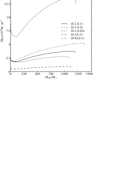
Figure 2: Plot of BH accretion rate $\dot{M}_{\text{BH}}$ against BH mass $M_{\text{BH}}$ for various pairs of values of the radiative and convective efficiencies ($\epsilon,\eta$). The fiducial values ($0.1,0.1$) correspond to the solid line. As expected, changing the radiative efficiency changes $\dot{M}_{\text{BH}}$ but leaves the overall structure unaffected. Decreasing $\eta$ causes the envelope to be hotter and denser in order to achieve the same luminosity shifting the discontinuities in the gradient of the accretion rate to later times.

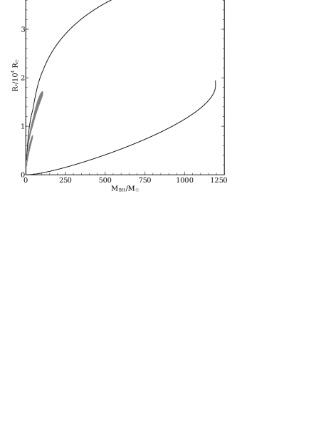
Figure 3: Radial location of convective boundaries and the Bondi radius for the fiducial run. The shaded regions are the radiative parts of the envelope. The outer solid lines show the extent of the hydrostatic envelope. The qualitative change in the locations of convective boundaries causes the discontinuities in the gradient of the accretion rate that are seen in Fig. 2. The outermost layer of the envelope is radiative (as it should be) but it is too narrow to be seen here.

What actually happens to the material in the cavity after the end of the hydrostatic evolution? Because we do not model it, we can only speculate. It appears that the entire envelope might be swallowed but it is not certain that this should be the case. The accretion flow is convective so there must be a combination of inward and outward flowing material within the Bondi radius. In the theoretical limit for a purely convective flow, the accretion rate is zero (Quataert & Gruzinov, 2000) and about half of the material is moving inward and half outward. If the flow is sustained then we might expect at least half of the cavity mass to be accreted. On the other hand the flow structure might change completely. The infalling material could settle into a disc and drive disc winds or jets so that the overall gain in mass is relatively small. The envelope is also convective and we expect equal masses of gas to be moving inward and outward. Hydrostatic equilibrium is presumably failing so the dynamics might change drastically here, too. Recently, Johnson et al. (2011) modeled the accretion on to massive BHs formed through direct collapse. They assumed that the BH accretes from a multi-colour black body disc after its quasi-star phase and found that, once the BH mass exceeds about $10^{4}\hbox{$\rm\thinspace\text{M}_{\sun}$}$, the accretion rate decreases due to radiative feedback. This result supports the case for a substantial decrease in the BH growth rate if a thin disc forms after the quasi-star phase but additional growth can occur during the transition to a new structure.

4 Final BH mass limit

We have not yet found a simple explanation for the existence of the upper limit to the BH mass in a quasi-star. In this section, we explore some theory that confirms the existence of such a limit and points towards possible mechanisms.

4.1 Loaded polytropes

Consider the equations of hydrostatic equilibrium and mass conservation truncated at some radius $r_{0}$ and loaded with some mass $M_{0}$ interior to that point. The equations are

$${\frac{dP}{dr}}=-\frac{Gm\rho(r)}{r^{2}}$$ (18)

and

$${\frac{dm}{dr}}=4\pi r^{2}\rho(r)$$ (19)

with the central boundary conditions $\left.m\right|_{r_{0}}=M_{0}$, where $r_{0}$ and $M_{0}$ are fixed. We scale the pressure and density using the usual polytropic assumptions

$$P=K\rho^{1+\frac{1}{n}}$$ (20)

and

$$\rho=\rho_{0}\theta^{n}\text{.}$$ (21)

We define the dimensionless radius by

$$r=\alpha\xi\text{,}$$ (22)

where

$$\alpha^{2}=\frac{(n+1)K}{4\pi G}\rho_{0}^{\frac{1}{n}-1}\text{.}$$ (23)

We scale the mass interior to a sphere of radius $r$ by defining

$$\phi(\xi)=\frac{m}{4\pi\rho_{0}\alpha^{3}}$$ (24)

(Huntley & Saslaw, 1975). The non-dimensional form of the equations is then

$${\frac{d\theta}{d\xi}}=-\frac{1}{\xi^{2}}\phi$$ (25)

and

$${\frac{d\phi}{d\xi}}=\xi^{2}\theta^{n}$$ (26)

with boundary conditions $\theta(\xi_{0})=1$ and $\phi(\xi_{0})=\phi_{0}$ (where, by definition, $\xi_{0}=r_{0}/\alpha$).

We can express $\phi_{\text{BH}}$ (the scaled BH mass) in terms of the inner radius by rescaling equation (2) as follows.

$$\xi_{0}=\frac{r_{0}}{\alpha} =\frac{2G}{\alpha}\frac{M_{\text{BH}}}{c_{s}^{2}}$$ (27)

$$=\frac{2G}{\alpha}4\pi\rho_{0}\alpha^{3}\phi_{\text{BH}}\frac{n}{(n+1)K\rho_{0}^{\frac{1}{n}}}$$ (28)

$$=2n\alpha^{2}\phi_{\text{BH}}\frac{4\pi G}{(n+1)K\rho_{0}^{\frac{1}{n}-1}}$$ (29)

$$=2n\phi_{\text{BH}}\text{.}$$ (30)

Similarly, we can derive the following relation for $M_{\text{cav}}$ from equation (5).

$$\phi_{\text{cav}} =\frac{\frac{8\pi}{3}\rho_{0}(\alpha\xi_{0})^{3}}{4\pi\rho_{0}\alpha^{3}}$$ (31)

$$=\frac{2}{3}\xi_{0}^{3}\text{.}$$ (32)

The scaled mass and radius boundary conditions are now related by

$$\phi_{0}\equiv\phi(\xi_{0})=\frac{1}{2n}\xi_{0}+\frac{2}{3}\xi_{0}^{3}\text{.}$$ (33)

Thus, for a given polytropic index $n$, we can choose a value $\xi_{0}$ and integrate the equations.

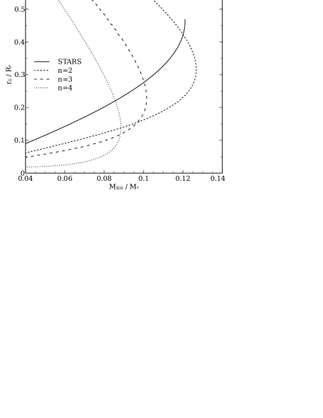
Figure 4: Plot of the ratio of BH mass against total mass against inner envelope radius to outer envelope radius. The double-valued curves correspond to polytropic solutions (with $n=2,3$ and $4$). The monotonic curve (solid line) represents the fiducial results. The polytropic models show the existence of an upper limit to the BH mass ratio. The fiducial results reach a similar limit, but the mass ratio cannot decrease, so the evolution terminates.

We integrated a sequence of solutions for $n=3$ and found that there exists a maximum value of $\phi_{\text{BH}}/\phi_{*}=0.102$, where $\phi_{*}$ is the scaled total mass of the quasi-star. The maximum occurs when $\xi_{0}=0.995$. We investigated polytropic indices between $2$ and $4$ and found a similar limit in all cases. For $n=2$ we found a maximum $\phi_{\text{BH}}/\phi_{*}=0.127$ when $\xi_{0}=1.012$ and for $n=4$ the maximum was $\phi_{\text{BH}}/\phi_{*}=0.089$ at $\xi_{0}=0.968$. Fig. 4 shows plots of the curves of the ratio of inner to outer envelope radius ($\xi_{0}/\xi_{*}$ in scaled variables, where $\xi_{*}$ is the outer radius of the envelope) against the BH fractional mass ($\phi_{\text{BH}}/\phi_{*}$ in scaled variables) for $n=2$, $3$ and $4$ together with our results for the fiducial model. The maximum mass ratio is clear in each curve. In principle, further hydrostatic solutions probably exist along the sequence computed by stars but they require that the BH mass decreases.

The conclusion we draw is that the models produced by the code come to a halt because no further realistic hydrostatic solutions can be found along the sequence. The discussion in this section, even though it does not immediately offer an explanation of why, thus indicates that such a limit does truly exist. The limit is robust in the sense that it exists at approximately the same ratio for all masses and does not depend on details such as opacity or energy transport (as long as the envelope is convective). The main dependence in real models is due to variation in the polytropic index.

4.2 The $U$–$V$ plane

It is known that (see Chandrasekhar, 1939, Section 4.8), if one has determined a solution $\theta(\xi)$ to the Lane-Emden equation, then $\theta^{\prime}(\xi^{\prime})\equiv C^{\frac{2}{n-1}}\theta(C\xi)$ is also a solution for an arbitrary constant $C$. By selecting appropriate variables that are invariant to such a transformation, one can find all the related solutions in a single calculation. Though a number of appropriate variables exist, many authors (such as Kimura, 1981; Horedt, 1987) use $U$ and $V$, defined below. Converting to the new variables also allows the analysis of solutions of the polytropic equation that do not extend to $\xi=0$ or contain the entire mass of the envelope. Physical solutions are restricted to positive $U$ and $V$. The first quadrant of the plane that they form is a useful tool for analyzing the behaviour of solutions.

We begin by defining

$$U=\frac{\xi^{3}\theta^{n}}{\phi}$$ (34)

and

$$V=\frac{\phi}{\xi\theta}\text{.}$$ (35)

Let us differentiate the logarithms of these variables with respect to $\xi$.

$$\frac{1}{U}{\frac{dU}{d\xi}} =\frac{3}{\xi}+\frac{n}{\theta}{\frac{d\theta}{d\xi}}-\frac{1}{\phi}{\frac{d\phi}{d\xi}}$$ (36)

$$=\frac{3}{\xi}-\frac{n\phi}{\theta\xi^{2}}-\frac{\xi^{2}\theta^{n}}{\phi}$$ (37)

$$=\frac{1}{\xi}(3-nV-U)$$ (38)

and

$$\frac{1}{V}{\frac{dV}{d\xi}} =-\frac{1}{\xi}-\frac{1}{\theta}{\frac{d\theta}{d\xi}}+\frac{1}{\phi}{\frac{d\phi}{d\xi}}$$ (39)

$$=-\frac{1}{\xi}+\frac{\phi}{\theta\xi^{2}}+\frac{\xi^{2}\theta^{n}}{\phi}$$ (40)

$$=\frac{1}{\xi}(-1+U+V)\text{.}$$ (41)

Dividing these two equations eliminates $\xi$ and allows us to write the first-order equation

$${\frac{dV}{dU}}=-\frac{V}{U}\left(\frac{U+V-1}{U+nV-3}\right)\text{.}$$ (42)

Polytropes that have zero mass and non-zero density at $\xi=0$ begin at $(U,V)=(3,0)$.

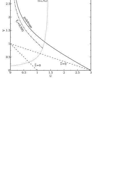
Figure 5: Some features of the $U$–$V$ plane for $n=3$. The dashed lines correspond to limiting values of $dV/dU$, as indicated on the plot. The dotted line shows the curve of central boundary conditions for the loaded polytropes described in Section 4.1, with BH mass increasing towards the top and right. The solid line shows the standard $n=3$ polytrope. The dash-dotted line is the loaded polytrope corresponding to the largest BH-envelope mass ratio. The intersection of the $dU/dV=0$ line and the curve of initial values corresponds well with the maximum accretion rate in in Fig. 2. It is interesting that the final model takes initial values approximately halfway between this point and the intersection with the $n=3$ polytrope.

Using the scaled boundary conditions in the previous section, we can determine the curve in the $U$–$V$ plane which corresponds to the interior values of our models. The relevant initial points are given by

$$U_{0}=\frac{\xi_{0}^{3}\theta_{0}^{n}}{\phi_{0}}=\xi_{0}^{2}\left(\frac{1}{2n}+\frac{2}{3}\xi_{0}^{2}\right)^{-1}$$ (43)

and

$$V_{0}=\frac{\phi_{0}}{\xi_{0}\theta_{0}}=\frac{1}{2n}+\frac{2}{3}\xi_{0}^{2}\text{.}$$ (44)

We can eliminate $\xi_{0}$ to give the curve of initial points in the $U$–$V$ plane.

$$V_{0}=\frac{3}{2n}\left(3-2U_{0}\right)^{-1}\text{.}$$ (45)

Different BH masses correspond to different points along this curve. A solution for a particular BH mass is then a curve going from the relevant point on the $(U_{0},V_{0})$ curve towards $U=0$.

Fig. 5 shows a number of features in the $U$–$V$ plane for $n=3$. Along the $dV/dU=0$ or $dU/dV=0$ lines, the solutions are horizontal or vertical, respectively, in the $U$–$V$ plane. All solutions bounded below by the $dU/dV=0$ have decreasing $U$ and increasing $V$ everywhere.

How do the points of interest correspond to our models? The intersection of the $dU/dV=0$ line and the $(U_{0},V_{0})$ curve corresponds to $\xi_{0}=0.835$, for which the BH-envelope mass ratio is $0.0953$. This appears to correspond to the point at which the accretion rate achieves its final local maximum. The dash-dotted line indicates the solution to the equations in Section 4.1 that has the largest BH-envelope mass ratio. The curve’s initial point appears to be about halfway between the intersections of the $(U_{0},V_{0})$ curve with the $dU/dV=0$ and with the polytropic solution. Though the mechanism behind the mass limit is not yet known, the analysis in this section shows that the limit is reproduced in the polytropic approximation, so the relevant physics is contained within mass conservation and hydrostatic equilibrium.

5 Further results

In Section 3, we established the basic qualitative structure and evolution of the quasi-star envelope. In this section, we explore their dependence on some of the parameters of the model.

5.1 Radiative and convective efficiencies

We first vary the accretion rate by adjusting the parameters $\epsilon$ and $\eta$. Fig. 2 shows the accretion history against BH mass for a number of parameter choices. Because the luminosity always settles on the same convection-limited rate, changing $\epsilon$ only rescales the accretion rate through equation (9) and has no effect on the structure. The final BH mass and intermediate properties are the same. The only difference is that the evolution takes longer for larger values of $\epsilon$.

Increasing the convective efficiency $\eta$ allows a greater flux to be radiated. Because it is a limiting factor, a larger value of $\eta$ allows a larger accretion rate for given interior conditions. In order to establish the same overall luminosity, the envelope must be less dense. This explains the different times at which the discontinuities in the gradient of the accretion rate appear.

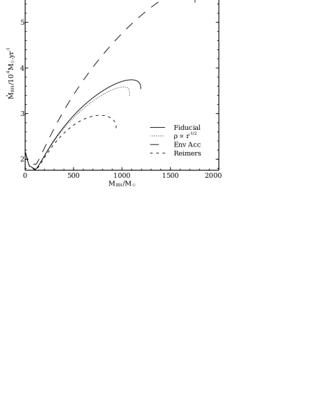
Figure 6: Plot of BH accretion rate $\dot{M}_{\text{BH}}$ against BH mass $M_{\text{BH}}$ for the fiducial run, a run with constant accretion on to the surface of the star (“Env Acc”), a run with a Reimers (1975) mass loss rate (“Reimers”) and a run with a shallower radial dependence of the interior density (“$\rho\propto r^{-1/2}$”). The Reimers rate leaves an envelope of about $7750\hbox{$\rm\thinspace\text{M}_{\sun}$}$ and the BH is proportionally smaller. The accreting envelope also leaves a proportionally scaled BH. A shallower radial dependence of the interior density leads to a smaller cavity mass and therefore a smaller interior density and accretion rate.

5.2 Cavity properties

The second property we adjust is the radial profile of the density inside the cavity. If the inward transport of angular momentum by advection and convection is greater than the outward transport by magnetic fields and other sources of viscosity, then the density profile tends towards $\rho(r)\propto r^{-\frac{1}{2}}$. Recomputing the cavity mass from equation (3) gives

$$M_{\text{cav}}=\frac{8\pi}{5}\rho_{0}r_{\text{B}}^{3}\text{.}$$ (46)

The quasi-star evolution is shown in Fig. 6. The smaller interior mass leads to a less evident density spike at all times. The decreased interior mass is subject to a lower mass limit for the BH. The final BH mass is $1077\hbox{$\rm\thinspace\text{M}_{\sun}$}$.

Although the change to the cavity properties affects the numerical results, there is no qualitative change to the quasi-star evolution. The evolution terminates owing to the same physical mechanism as is analysed in Section 4.

5.3 Envelope mass loss and gain

To illustrate the effect of a net accretion rate on to the surface of the envelope, Fig. 6 shows the evolution of the fiducial run if the envelope is accreting at a constant rate of $2\times 10^{-3}\hbox{$\hbox{$\rm\thinspace\text{M}_{\sun}$}\rm\thinspace yr^{-1}\,$}$. Although this rate initially exceeds the quasi-star’s Eddington limit, such rapid infall is believed to occur as long as the bars-within-bars mechanism is transporting material towards the centre of the pregalactic cloud. Once the surface temperature of the quasi-star decreases below about $8000\rm\thinspace K$, the Eddington limit becomes much larger owing to the decreasing opacity. The accreted mass is simply added to the surface value of the mass co-ordinate and no additions are made to any other equations. In particular, we do not include a ram pressure at the surface. The only qualitative change to the evolution is that it takes longer than if the total mass had been held constant at the same final value of $17\,540\hbox{$\rm\thinspace\text{M}_{\sun}$}$. The final BH mass is subject to the same ratio limit so a larger final envelope permits a larger final BH.

To investigate the effect of mass loss we use a Reimers rate (Reimers, 1975). It is an empirical relation to describe mass loss in red giants. The mass-loss rate is

$$\dot{M}_{\text{loss}}=4\times 10^{-13}\frac{L_{*}R_{*}}{M_{*}}\frac{\hbox{$\rm\thinspace\text{M}_{\sun}$}}{\hbox{$\rm\thinspace L_{\sun}$}\hbox{$\rm\thinspace\text{R}_{\sun}$}}\text{.}$$ (47)

Fig. 6 shows the evolution for quasi-star envelopes with this prescription. The mass loss is significant but, again, no qualitative change in the results is seen. The limit holds and the BH is slightly smaller, precisely in proportion with the decrease in the mass of the envelope.

5.4 Initial envelope mass

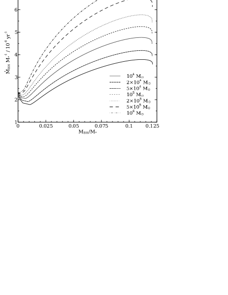
Figure 7: Plot of the evolution of quasi-stars of different total masses. The BH mass and accretion rates have been divided by the total quasi-star mass to illustrate the consistency of the upper mass ratio limit of $0.119$ and the slight dependence of the accretion rate with quasi-star mass. Because larger quasi-stars permit greater scaled accretion rates, they have shorter hydrostatic lifetimes.

The structure of the envelope appears to be chiefly dependent on the ratio of envelope mass to BH mass. We constructed a set of models with initial total masses $M_{*}/\hbox{$\rm\thinspace\text{M}_{\sun}$}=10^{4},2\times 10^{4},5\times 10^{4},10^{5},2\times 10^{5},5\times 10^{5}$, and $10^{6}$ to confirm this and explore how the temporal evolution of the envelopes is affected by total mass.

Fig. 7 shows the evolution of the various envelopes with the BH mass and accretion rate divided by the quasi-star masses. We note that the fractional upper BH mass limit holds for all the quasi-star masses in this range. Also, the temperature profiles by mass of the envelopes depend almost exclusively on the BH-envelope mass ratio. The variation in inner or surface temperature, for a given mass ratio, with respect to the total mass of the quasi-star is less than 0.05 per factor of ten in the total mass.

The density and radius profiles are more strongly dependent on the mass of the envelope. We find that, for a given mass ratio and once the entire envelope has become convective, the following approximate relations hold for the properties of two quasi-stars of different masses (denoted by subscripts 1 and 2).

$$\left(\frac{R_{*,1}}{R_{*,2}}\right)=\left(\frac{M_{*,1}}{M_{*,2}}\right)^{0.54}\text{,}$$ (48)

$$\left(\frac{\rho_{0,1}}{\rho_{0,2}}\right)=\left(\frac{M_{*,1}}{M_{*,2}}\right)^{-0.66}\text{,}$$ (49)

and

$$\left(\frac{\dot{M}_{\text{BH},1}}{\dot{M}_{\text{BH},2}}\right)=\left(\frac{M_{*,1}}{M_{*,2}}\right)^{1.14}\text{.}$$ (50)

For example, compared to a quasi-star of mass $10^{4}\hbox{$\rm\thinspace\text{M}_{\sun}$}$ at the same BH-envelope mass ratio, a $10^{5}\hbox{$\rm\thinspace\text{M}_{\sun}$}$ quasi-star will have an outer radius that is $10^{0.54}=3.47$ times greater, an interior density that is $10^{0.66}=4.57$ times smaller and a mass accretion rate that is $10^{1.14}=13.8$ times greater.

The final relation implies that the lifetime of a quasi-star scales as $\tau_{\text{QS}}\propto M_{*}^{-0.14}$ so larger quasi-stars have slightly shorter hydrostatic lifetimes. Fig. 7 shows how the BH-envelope mass ratio for which the entire envelope is convective also depends on the envelope mass. This has a small effect on the lifetime of the quasi-stars. By fitting a straight line to the $\log\tau_{\text{QS}}$–$\log M_{*}$ relation for the seven models here, we find that the lifetimes scale as $\tau_{\text{QS}}\propto M_{*}^{-0.13}$. More precisely, we find

$$\log_{10}\tau_{\text{QS}}=-0.126\log_{10}M_{*}+7.12$$ (51)

Note that $M_{*}$ here denotes the initial mass of the quasi-star. In all other relations $M_{*}$ slowly decreases during the quasi-star’s evolution owing to the mass-energy lost as radiation.

5.5 Comparison with Begelman et al. (2008)

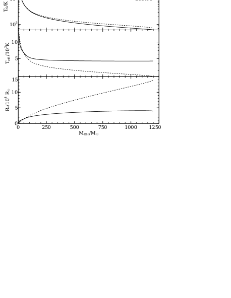
Figure 8: Comparison of analytic estimates of BRA08 (dashed lines) against results for our fiducial run (solid lines) for interior temperature (top), surface temperature (middle) and envelope radius (bottom). BRA08’s estimate of the interior temperature is accurate but those for the photospheric temperature and envelope radius become increasingly inaccurate as the BH grows.

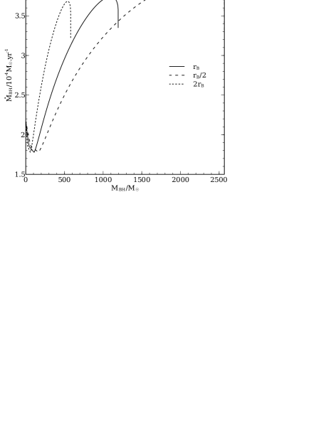
Figure 9: Plot of BH accretion rate $\dot{M}_{\text{BH}}$ against BH mass $M_{\text{BH}}$ for different choices of the inner boundary radius. The various values of $r_{0}$ lead to qualitatively similar results but the quantitative evolution is strongly affected.

BRA08 have estimated some envelope properties presuming that the envelope is described by an $n=3$ polytrope. Their estimates are made in terms of an overall accretion efficiency parameter $\alpha_{\text{BRA}}$ which is determined by numerical factors in the accretion rate including the radiative efficiency, convective efficiency and adiabatic index. Because our adiabatic index is not fixed, we have calibrated $\alpha_{\text{BRA}}$ using the BH luminosity (equation 3 of BRA08). To compare the fiducial run, we selected $\alpha_{\text{BRA}}\approx 0.257$ which makes their analytical BH luminosity accurate to within 0.2 per cent over the entire evolution.

We compare the following estimates for the inner temperature, photospheric temperature and envelope radius (equations 7, 11 and 10 of BRA08, respectively).

$$T_{0}=1.4\times 10^{4}\left(\frac{L}{L_{\text{Edd}}}\right)^{\frac{2}{5}}\left(\alpha_{\text{BRA}}\frac{M_{\text{BH}}^{2}}{\mathrm{M}_{\odot}^{2}}\right)^{-\frac{2}{5}}\left(\frac{M_{*}}{\hbox{$\rm\thinspace\text{M}_{\sun}$}}\right)^{\frac{7}{10}}\rm\thinspace K\text{,}$$ (52)

$$T_{\text{eff}}=1.0\times 10^{3}\left(\frac{L}{L_{\text{Edd}}}\right)^{\frac{9}{20}}\left(\alpha_{\text{BRA}}\frac{M_{\text{BH}}^{2}}{\mathrm{M}_{\odot}^{2}}\right)^{-\frac{1}{5}}\left(\frac{M_{*}}{\hbox{$\rm\thinspace\text{M}_{\sun}$}}\right)^{\frac{7}{20}}\rm\thinspace K$$ (53)

and

$$R_{*}=4.3\times 10^{14}\left(\frac{L}{L_{\text{Edd}}}\right)^{-\frac{2}{5}}\left(\alpha_{\text{BRA}}\frac{M_{\text{BH}}^{2}}{\mathrm{M}_{\odot}^{2}}\right)^{\frac{2}{5}}\left(\frac{M_{*}}{\hbox{$\rm\thinspace\text{M}_{\sun}$}}\right)^{\frac{1}{5}}\rm\thinspace cm\text{.}$$ (54)

Here, $L_{\text{Edd}}=4\pi GcM/\kappa$ is the Eddington luminosity. BRA08 computed this using the opacity at the boundary of the convective zone but such estimates differ by a factor of the order of $\kappa/\kappa_{\text{es}}$ when compared with our results. Our comparison is made using the Eddington limit with opacity $\kappa_{\text{es}}=0.34\hbox{$\rm\thinspace cm^{2}\,$}\hbox{$\rm\thinspace g^{-1}\,$}$.

In Fig. 8, we plot the three estimates against the results from our fiducial run. The estimate for the interior temperature is accurate to within 20 per cent. The deviation grows as the approximation of the envelope to an $n=3$ polytrope becomes increasingly less accurate.

The estimate for the photospheric temperature is highly inaccurate. At the end of the run the estimated photospheric temperature is about $2400\rm\thinspace K$ compared to the model result of about $4500\rm\thinspace K$. Because the BH luminosity estimate is very accurate, it then follows that the envelope radius is inaccurate. The surface luminosity must be related by $L_{*}=\pi acR_{*}^{2}T_{\text{eff}}^{4}$. This is confirmed in the bottom panel of Fig. 8.

BRA08 argue that quasi-star evolution terminates owing to the opacity at the edge of the convection zone increasing. The increased opacity causes the envelope to expand and the opacity increases further. The envelope then expands further and the process is claimed to run away. BRA08 refer to this process as the opacity crisis. Our results do not terminate for this reason. Similar behaviour does occur at the beginning of the evolution while the photospheric temperature is greater than $10^{4}\rm\thinspace K$ but it does not disperse the quasi-star. For most of a quasi-star’s evolution, the opacity at the convective boundary is already beyond the H-ionization peak and is decreasing as the BH grows.

6 Sensitivity to the inner boundary

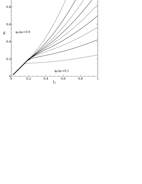
Figure 10: Contours of $\phi_{0}/\phi_{*}$ for the models calculated for each pair of initial conditions $(\xi_{0},\phi_{0})$ in the plane. There is a clear boundary along $\phi_{0}=\xi_{0}$ near the origin. Solutions above this line must have negligibly small envelopes by mass.

Besides the physical parameters of the models, we have also considered the effect of changing the inner boundary radius. Fig. 9 shows the evolution of quasi-stars where the inner radius was changed to half and twice the Bondi radius. The final BH mass is strongly affected although the evolution is qualitatively similar. The results of our polytropic analysis in Section 4 are also affected in a consistent manner. Although reasonable, our choice of inner radius is somewhat arbitrary and critical in deciding the quantitative evolution of the quasi-star. A self-consistent model to determine the appropriate value of $r_{0}$ is thus highly desirable but none is yet available. We continue to seek a suitable resolution to this issue.

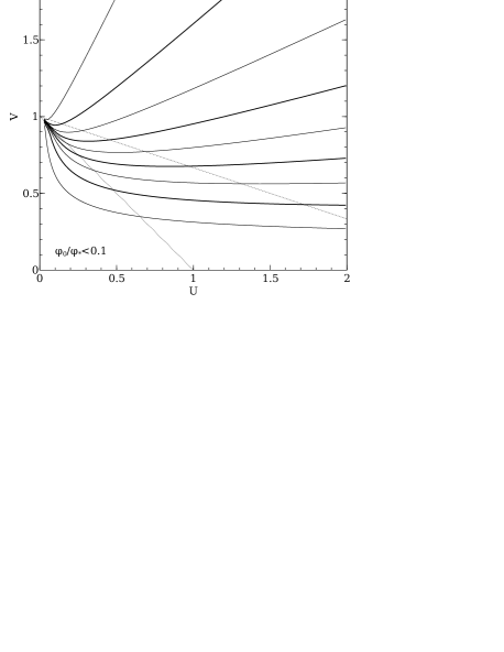
Figure 11: Contours of $\phi_{0}/\phi_{*}$ for the models calculated for each pair of initial conditions $(U_{0},V_{0})$ in the plane. The boundary in Fig. 10 corresponds to the critical point (0,1).

The sensitivity of the models to the inner boundary precipitated further interesting results. We note that the final BH mass is scaled by approximately the same factor as the inner radius. That is, if $r_{0}$ is doubled, the BH reaches about half the final mass that it reached before. If the material properties at the inner boundary were largely unchanged, this would imply that the inner radius at the termination of the runs is approximately the same. The output from the models indicates that $r_{0}/\hbox{$\rm\thinspace\text{R}_{\sun}$}$ in the final reliable model of each run in Fig. 9 is approximately $2.05\times 10^{4}$, $1.94\times 10^{4}$ and $1.79\times 10^{4}$ for $r_{0}=2r_{\text{B}}$, $r_{\text{B}}$ and $r_{\text{B}}/2$. This indicates that the limit determined for the polytropic models in Section 4 may be related more strongly to the ratio of inner to outer radius than the ratio of interior to total mass.

It may appear from Fig. 4 that the limiting radius ratios for the STARS output and the polytropic models are inconsistent. The discrepancy is due to the ionization zones inside the envelope. It is also difficult to identify the appropriate values because the inner and outer radii are changing most rapidly at the end of the evolution. Using the last models in each run of Section 5.4 that have converged in thermal equilibrium, the limit is approximately $r_{0}/R_{*}\approx 0.460$.

We additionally found that we could not construct model envelopes for $r_{0}\la 0.3r_{\text{B}}$ and find that this is reflected in the polytropic models. To construct Fig. 10 we have calculated the ratio $\phi_{0}/\phi_{*}$ for each $(\xi_{0},\phi_{0})$ pair in the plane and plotted contours from $0$ to $1$ in steps of $0.1$. Near the origin, there is a clear boundary along the line $\phi_{0}=\xi_{0}$. The boundary softens for larger values of $\phi_{0}$ and $\xi_{0}$. For small $\xi_{0}$, models above the boundary necessarily have $\phi_{0}/\phi_{*}\approx 1$. In other words, any model with a sufficiently small inner boundary must have an appropriately small envelope.

The limit becomes clearer when plotted in the $U$–$V$ plane discussed in Section 4.2. We have done so in Fig. 11. The contours are divided across the point (0,1). This is a critical point in the $U$–$V$ plane for all polytropic indices. It is neutrally stable in the direction (1,-1) and unstable along the $V$-axis i.e. (0,1).

The present analysis thus provides several important results. First, the choice of inner radius is crucial to determining the evolution of the envelopes. The Bondi radius is a reasonable choice but there is no evidence to confirm that it is the correct one. Secondly, the limit determined in Section 4 seems more strongly related to the radius ratio than the mass ratio. This was not obvious at first because there was no apparent reason to modify the inner radius. Thirdly, there is a limit to the smallest value that can be chosen for the inner radius.

7 Conclusion

We have modified the Cambridge stars stellar evolution code to model the evolution of quasi-star envelopes. Our first new result is the existence of a robust upper limit on the ratio of inner BH mass to the total mass, equal to about $0.119$, of the system in hydrostatic equilibrium. The limit is reflected in solutions of the Lane-Emden equation, modified for the presence of a point mass interior to some specific boundaries. After considering variation of the inner radius, this limit is possibly better interpreted as a limit to the ratio of inner radius to envelope radius. The value of the limit from the STARS output is about $0.46$.

All the evolutionary runs here terminate once the limit is reached. It is difficult to say what happens to the BH and envelope after the hydrostatic evolution ends. Some of the material within the Bondi radius has begun accelerating towards the BH so we expect that it can be captured by the BH. The remaining material may be accreted or expelled, depending on the liberation of energy from the material that does fall inwards. After the BH has evolved through the quasi-star phase, it is probably limited to accreting at less than the Eddington limit for the BH.

The models presented are crucially sensitive to the choice of inner boundary radius and the results should be treated with due caution. While the Bondi radius used here is reasonable, we continue to seek a less arbitrary set of boundary conditions.

In light of these results, it appears that quasi-stars produce BHs that are on the order of at least $0.1$ of the mass of the quasi-star and around $0.5$ if all the material within the inner radius is accreted. For conservative parameters, this growth occurs within a few million years after the BH initially forms. Realistic variations in the parameters (e.g. larger initial mass, lower radiative efficiency) lead to shorter lifetimes. Such BHs could easily reach masses exceeding $10^{9}\hbox{$\rm\thinspace\text{M}_{\sun}$}$ early enough in the Universe to power high-redshift quasars.

References

- Appenzeller & Fricke (1971) Appenzeller I., Fricke K., 1971, A&A, 12, 488
- Begelman (1978) Begelman M. C., 1978, MNRAS, 184, 53
- Begelman (2010) Begelman M. C., 2010, MNRAS, 402, 673
- Begelman & Shlosman (2009) Begelman M. C., Shlosman I., 2009, ApJL, 702, L5
- Begelman et al. (2006) Begelman M. C., Volonteri M., Rees M. J., 2006, MNRAS, 370, 289
- Begelman et al. (2008) Begelman M. C., Rossi E. M., Armitage P. J., 2008, MNRAS, 387, 1649 (BRA08)
- Bond et al. (1984) Bond J. R., Arnett W. D., Carr B. J., 1984, ApJ, 280, 825
- Bondi (1952) Bondi H., 1952, MNRAS, 112, 195
- Bromm & Larson (2004) Bromm V., Larson R. B., 2004, ARA&A, 42, 79
- Chandrasekhar (1939) Chandrasekhar S., 1939, An Introduction to the Study of Stellar Structure. Chicago Univ. Press, Chicago
- Clark et al. (2008) Clark P. C., Glover S. C. O., Klessen R. S., 2008, ApJ, 672, 757
- Cox & Giuli (1968) Cox J. P., Giuli R. T., 1968, Principles of Stellar Structure. Gordon & Breach, New York
- Devecchi & Volonteri (2009) Devecchi B., Volonteri M., 2009, ApJ, 694, 302
- Dijkstra et al. (2008) Dijkstra M., Haiman Z., Mesinger A., Wyithe J. S. B., 2008, MNRAS, 391, 1961
- Eddington (1918) Eddington A. S., 1918, ApJ, 48, 205
- Eggleton (1971) Eggleton P. P., 1971, MNRAS, 151, 351
- Eggleton (1972) Eggleton P. P., 1972, MNRAS, 156, 361
- Eggleton (1973) Eggleton P. P., 1973, MNRAS, 163, 279
- Eggleton et al. (1973) Eggleton P. P., Faulkner J., Flannery B. P., 1973, A&A, 23, 325
- Eldridge & Tout (2004) Eldridge J. J., Tout C. A., 2004, MNRAS, 348, 201
- Fan et al. (2006) Fan X. et al., 2006, AJ, 131, 1203
- Flammang (1984) Flammang R. A., 1984, MNRAS, 206, 589
- Fowler (1964) Fowler W. A., 1964, Rev. Modern Phys., 36, 545
- Freese et al. (2008) Freese K., Bodenheimer P., Spolyar D., Gondolo P., 2008, ApJL, 685, L101
- Fryer et al. (2001) Fryer C. L., Woosley S. E., Heger A., 2001, ApJ, 550, 372
- Horedt (1987) Horedt G. P., 1987, A&A, 177, 117
- Huntley & Saslaw (1975) Huntley J. M., Saslaw W. C., 1975, ApJ, 199, 328
- Itoh et al. (1996) Itoh N., Hayashi H., Nishikawa A., Kohyama Y., 1996, ApJS, 102, 411
- Jiang et al. (2008) Jiang L. et al., 2008, AJ, 135, 1057
- Johnson & Bromm (2007) Johnson J. L., Bromm V., 2007, MNRAS, 374, 1557
- Johnson et al. (2011) Johnson J. L., Khochfar S., Greif T. H., Durier F., 2011, MNRAS, 410, 919
- Kimura (1981) Kimura H., 1981, PASJ, 33, 273
- King & Pringle (2006) King A. R., Pringle J. E., 2006, MNRAS, 373, L90
- Langer (1997) Langer N., 1997, in Nota A., Lamers H., eds, ASP Conf. Ser., Vol. 120, Luminous Blue Variables: Massive Stars in Transition. p. 83
- Lodato & Natarajan (2006) Lodato G., Natarajan P., 2006, MNRAS, 371, 1813
- Loeb & Rasio (1994) Loeb A., Rasio F. A., 1994, ApJ, 432, 52
- Milosavljević et al. (2009) Milosavljević M., Couch S. M., Bromm V., 2009, ApJL, 696, L146
- Narayan et al. (2000) Narayan R., Igumenshchev I. V., Abramowicz M. A., 2000, ApJ, 539, 798
- Ohkubo et al. (2006) Ohkubo T., Umeda H., Maeda K., Nomoto K., Suzuki T., Tsuruta S., Rees M. J., 2006, ApJ, 645, 1352
- Pols et al. (1995) Pols O. R., Tout C. A., Eggleton P. P., Han Z., 1995, MNRAS, 274, 964
- Quataert & Gruzinov (2000) Quataert E., Gruzinov A., 2000, ApJ, 539, 809
- Regan & Haehnelt (2009) Regan J. A., Haehnelt M. G., 2009, MNRAS, 393, 858
- Reimers (1975) Reimers D., 1975, Mem. Soc. R. Sci. Liege, 8, 369
- Schleicher et al. (2010) Schleicher D. R. G., Spaans M., Glover S. C. O., 2010, ApJL, 712, L69
- Shang et al. (2010) Shang C., Bryan G. L., Haiman Z., 2010, MNRAS, 402, 1249
- Shapiro (2004) Shapiro S. L., 2004, in Ho, L. C., ed., Carnegie Observatories Astroph. Ser., Coevolution of Black Holes and Galaxies. Cambridge Univ. Press, Cambridge, p. 103
- Shlosman et al. (1989) Shlosman I., Frank J., Begelman M. C., 1989, Nat, 338, 45
- Spaans & Silk (2006) Spaans M., Silk J., 2006, ApJ, 652, 902
- Spolyar et al. (2008) Spolyar D., Freese K., Gondolo P., 2008, Phys. Rev. Lett., 100, 051101
- Tegmark et al. (1997) Tegmark M., Silk J., Rees M. J., Blanchard A., Abel T., Palla F., 1997, ApJ, 474, 1
- Thorne & Żytkow (1977) Thorne K. S., Żytkow A. N., 1977, ApJ, 212, 832
- Volonteri (2010) Volonteri M., 2010, A&AR, 18, 279
- Willott et al. (2010) Willott C. J. et al., 2010, AJ, 139, 906
- Wise et al. (2008) Wise J. H., Turk M. J., Abel T., 2008, ApJ, 682, 745