Permutation orbifolds of heterotic Gepner models

Abstract

We study orbifolds by permutations of two identical N=2 minimal models within the Gepner construction of four dimensional heterotic strings. This is done using the new N=2 supersymmetric permutation orbifold building blocks we have recently developed. We compare our results with the old method of modding out the full string partition function. The overlap between these two approaches is surprisingly small, but whenever a comparison can be made we find complete agreement. The use of permutation building blocks allows us to use the complete arsenal of simple current techniques that is available for standard Gepner models, vastly extending what could previously be done for permutation orbifolds. In particular, we consider $(0,2)$ models, breaking of $SO(10)$ to subgroups, weight-lifting for the minimal models and B-L lifting. Some previously observed phenomena, for example concerning family number quantization, extend to this new class as well, and in the lifted models three family models occur with abundance comparable to two or four.

                                                                                                       NIKHEF/2011-004

1 Introduction

Heterotic string theory [1] is the oldest approach towards the construction of the standard model in string theory. It owes its success to the fact that the gross features of the standard model appear to come out nearly automatically: families of chiral fermions in representations that are structured as in $SO(10)$-based GUT models. Presumably we know only a very small piece of this landscape of perturbative heterotic strings. Several computational methods are available, based either on space-time geometry or world-sheet conformal field theory. The latter category can be further subdivided into free and interacting field theory methods. But all these methods have obvious but inestimable limitations, making it difficult to determine how much of the heterotic landscape has really been explored so far.

In the case of the conformal field theory (CFT) methods [2], these limitations are due to the constraints imposed by world-sheet supersymmetry and modular invariance, for which we only know some classes of special solutions. A general heterotic CFT consists of a right-moving sector that has $N=2$ world-sheet supersymmetry and a non-supersymmetric left-moving sector. Most existing work has been limited either to free CFTs (bosons, fermions or orbifolds) for these two sectors, or to interacting CFTs where the bosonic sector is essentially a copy of the fermionic one. Furthermore the interacting CFTs themselves have mostly been limited to tensor products of $N=2$ minimal models [3, 4].

Already in the late eighties of last century ideas were implemented to reduce some of these limitations of interacting CFTs. Instead of minimal models, Kazama-Suzuki models were used [5]. Another extension was to consider permutation orbifolds of $N=2$ minimal models [6, 7]. But both of these ideas could only be analyzed in a very limited way themselves. The real power of interacting CFT construction comes from the use of simple current invariants [8, 9, 10, 11, 12], which greatly enhance the number and scope of the possible constructions. In particular the left-right symmetry of the original Gepner models could be broken by considering asymmetric simple current invariants [13], allowing for example a breaking of the canonical $E_{6}$ subgroup to $SO(10)$, $SU(5)$, Pati-Salam models or even just the standard model (with some additional factors in the gauge group). However, precisely this powerful tool is not available at present in either Kazama-Suzuki models or permutation orbifolds. The original computations were limited to diagonal invariants, where with a combination of a variety of tricks the spectrum could be obtained. Up to now, all that is available in the literature is a very short list of Hodge numbers and singlets for $(2,2)$ spectra with $E_{6}$ gauge groups [6, 7, 14, 15]. To use the full power of simple current methods we need to know the exact CFT spectrum and the fusion rules of the primary fields of the building blocks. The former has never been worked out for Kazama-Suzuki models, and the latter was not available for permutation orbifolds until last year. Using pioneering work by Borisov, Halpern and Schweigert [16] and an extension of these results to fixed point resolution matrices [17, 18, 19] we have constructed the $\mathbb{Z}_{2}$ permutation orbifolds of $N=2$ minimal models [20]. These can now be used as building blocks in heterotic CFT constructions, on equal footing, and in combination with all other building blocks, such as the minimal models themselves and free fermions. Furthermore we can now for the first time apply the full simple current machinery in exactly the same way as for the minimal models.

Meanwhile, another method was added to this toolbox, allowing us to advance a bit more deeply into the heterotic landscape, and away from free or symmetric CFTs. This is called “heterotic weight lifting” [21], a replacement of $N=2$ building blocks in the bosonic sector by isomorphic (in the sense of the modular group) $N=0$ building blocks (more precisely, replacing $N=2$ building blocks together with the extra $E_{8}$ factor). This method requires knowledge of the exact CFT spectrum, which indeed we have. A variant of this idea is the replacement of the $U(1)_{B-L}$ factor ($\times E_{8}$) by an isomorphic CFT. This has been called “B-L lifting”.

In a series of papers [22, 23, 24, 25], all combinations of the aforementioned tools were applied to Gepner models. The focus of this work was on three important features of the spectra of these models: do the chiral fermions really form standard model families, do the non-chiral fermions respect standard model charge quantization, and do three families occur reasonably often. The answers to these questions can be summarized as “sometimes, no, and yes”. A substantial fraction of the chiral spectra with broken GUT symmetry is organized in standard model families, but the rest has chiral exotics. In the exact spectrum there are almost always vector-like states which violate the charge quantization rules of the standard model and hence would lead to light fractionally charged particles, unless they are lifted by moving into moduli space, away from the special RCFT points. The conclusion on the number of families was a bit more optimistic. Despite the difficulties of standard Gepner models to yield three families, this problem disappears if one moves away from symmetric CFTs. Just using asymmetric MIPFs is not sufficient, but if one really makes the left and right CFTs distinct by using heterotic weight lifting or B-L lifting one obtains a normal, more or less exponential distribution $\propto e^{-\alpha N}$ with $\alpha$ in the range $.2-.3$, where $N$ is the number of families. The number three is not strongly suppressed in these distributions, and occurs for a total of about $15\%$ of the $N$-family models.

The purpose of this paper is to put all these ingredients together using permutation orbifolds of $N=2$ minimal models as building blocks in combination with minimal models. We want to do this for the following reasons:

• Check the consistency of the permutation orbifold CFTs we presented in [20]. Chiral heterotic spectra are very sensitive to the correctness of conformal weights and ground state dimensions of the CFT, as well as the correctness of the simple current orbits. This is especially true for weight-lifted spectra, because they have non-trivial Green-Schwarz anomaly cancellations.

• Compare our results with those of previous work on permutation orbifolds [6, 7]. These results were obtained using a rather different method, by applying permutations directly to complete heterotic string spectra.

• Check if the aforementioned trends on fractional charged and family number are confirmed also in the class of permutation orbifolds.

• Add a few more items to the growing list of potentially interesting three-family interacting CFT models.

The key ingredient of the present work is is our previous paper [20], where we studied permutations, together with extensions in all possible order, and found very interesting novelties. For example, we determined how to construct a supersymmetric permutation of minimal models: in particular, the world-sheet-supersymmetry current in the supersymmetric orbifold turns out to be related to the anti-symmetric representation of the world-sheet-supersymmetry current of the original minimal model. When the symmetric representation is used, instead, one ends up with a conformal field theory, which is isomorphic to the supersymmetric orbifold, but it is not supersymmetric itself.

In the extended permuted orbifolds so-called exceptional simple currents appear, which originate from off-diagonal representations. Generically, there are many of them, depending on the particular model under consideration, and they do not have fixed points. However, when and only when the “level” is equal to $k=2$ mod $4$, four of all these exceptional currents do admit fixed points. As a consequence, in those cases the knowledge of the modular $S$ matrix is plagued by the existence of non-trivial and unknown $S^{J}$ matrices (one $S^{J}$ matrix for each exceptional current $J$). The full set of $S^{J}$ matrices is available for standard $\mathbb{Z}_{2}$ orbifolds (see [17, 18, 19]), but not for their (non)supersymmetric extensions, due to these four exceptional currents with fixed points. This is known as the fixed point resolution problem [26, 27, 28, 29, 30, 31]. The knowledge of the full set of the $S^{J}$ matrices is more important in orientifold models [32, 33, 34] than in heterotic strings, because in the former case one cannot even compute spectra if these matrices are not known.

In this paper we consider permutations in Gepner models. One starts with Gepner’s standard construction where the internal CFT is a product of $N=2$ minimal models. Sometimes there are (at least) two $N=2$ identical factors in the tensor product. When it is the case, we can replace these two factors with their permutation orbifold. Moreover, one also has to impose space-time and world-sheet supersymmetry, which is achieved by suitable simple-current extensions.

The plan of the paper is as follows. In section 2 we start reviewing the permutation orbifold, which is the main idea used in this paper. In section 3 we review the standard constructions of Heterotic Gepner models. In section 4 we review the main ingredients and the most relevant results of $\mathbb{Z}_{2}$ permutation orbifolds when applied to $N=2$ minimal models. In section 5 we describe the heterotic weight lifting and the B-L lifting procedures, which allow us to replace the trivial $E_{8}$ factor plus either one $N=2$ minimal model or the $U(1)_{B-L}$ with a different CFT, which has identical modular properties, in the bosonic (left) sector. In section 6 we compare our results on (2,2) spectra with the known literature. In section 7 we present our phenomenological results concerning the family number distributions, gauge groups, fractional charges and other relevant data. In appendix A we derive a few facts about simple current invariants. Appendix A.2 contains tables summarizing the main results for the four cases (standard Gepner models and the three kinds of lifts).

2 Permutation orbifold

In this section let us recall a few properties of the generic permutation orbifold [16], restricted to the $\mathbb{Z}_{2}$ case:

$$\mathcal{A}_{\rm perm}\equiv\mathcal{A}\times\mathcal{A}/\mathbb{Z}_{2}\,.$$ (2.1)

If $c$ is the central charge of $\mathcal{A}$, then the central charge of $\mathcal{A}_{\rm perm}$ is $2c$. The typical weights of the fields are:

• $h_{(i,\xi)}=2h_{i}$

• $h_{\langle i,j\rangle}=h_{i}+h_{j}$

• $h\widehat{(i,\xi)}=\frac{h_{i}}{2}+\frac{c}{16}+\frac{\xi}{2}$

for diagonal, off-diagonal and twisted representations. Sometimes it can happen that the naive ground state has dimension zero: then one must go to its first non-vanishing descendant whose weight is incremented by integers.

The permutation orbifold characters $X$ are related to the characters $\chi$ of the mother theory $\mathcal{A}$ in the following way [16]:

$$X_{\langle i,j\rangle}(\tau) = \chi_{i}(\tau)\cdot\chi_{j}(\tau)$$ (2.2a)

$$X_{(i,\xi)}(\tau) = \frac{1}{2}\chi_{i}^{2}(\tau)+e^{i\pi\xi}\frac{1}{2}\chi_{i}(2\tau)$$ (2.2b)

$$X_{\widehat{(i,\xi)}}(\tau) = \frac{1}{2}\chi_{i}(\frac{\tau}{2})+e^{-i\pi\xi}\,T_{i}^{-\frac{1}{2}}\,\frac{1}{2}\chi_{i}(\frac{\tau+1}{2})$$ (2.2c)

where $T_{i}^{-\frac{1}{2}}=e^{-i\pi(h_{i}-\frac{c}{24})}$. The character expansion:

$$\chi(\tau)=q^{h_{\chi}-\frac{c}{24}}\,\sum_{n=0}^{\infty}d_{n}q^{n}\qquad\qquad({\rm with}\,\,q=e^{2i\pi\tau})$$ (2.3)

(the $d_{n}$’s are non-negative integers) implies a similar expansion for the $X$:

$$X(\tau)=q^{h_{X}-\frac{c}{12}}\,\sum_{n=0}^{\infty}D_{n}q^{n}$$ (2.4)

where the $D_{n}$’s are expressed in terms of the $d_{n}$’s as follows:

$$D^{\langle i,j\rangle}_{k} = \sum_{n=0}^{k}d_{n}^{(i)}\,d_{k-n}^{(j)}$$ (2.5a)

$$D^{(i,\xi)}_{k} = \frac{1}{2}\sum_{n=0}^{k}d_{n}^{(i)}\,d_{k-n}^{(i)}+\left\{\begin{array}[]{lr}0&{\rm if}\,\,k={\rm odd}\\ \frac{1}{2}\,e^{i\pi\xi}\,d_{\frac{k}{2}}^{(i)}&{\rm if}\,\,k={\rm even}\end{array}\right.$$ (2.5d)

$$D^{\widehat{(i,\xi)}}_{k} = d_{2k+\xi}^{(i)}$$ (2.5e)

Using these characters, one can compute their modular transformation and find the orbifold $S$ matrix. It was determined in [16] and will be referred to as $S^{BHS}$. In theories where the permutation orbifold is extended by means of simple currents, one has to face the problem of fixed point resolution, namely one has to determine a set of “$S^{J}$ matrices”, one for each simple current $J$ [27]. For standard permutation orbifolds, it was shown in [17] that the simple currents can be only of diagonal type, i.e. $(J,\psi)$ where $J$ is a simple current of the mother theory and $\psi=0$ or $1$ for $\mathbb{Z}_{2}$ orbifolds. This set of matrices was determined in [19]. This fixed point resolution plays a crucial rôle in determining the fusion rules of the supersymmetric permutation orbifold, as explained in [20]. However, we will not need the explicit formulas for the fixed point resolution matrices in the present paper, and therefore we will not present them here.

3 Heterotic Gepner models

In this section we review the construction of four-dimensional heterotic string theory. The starting point is a set of bosons $X^{\mu}$ ($\mu=0,\dots,3$) for both the right and left movers, a right-moving set of NSR fermions $\psi^{\mu}$, plus corresponding ghosts, and an internal CFT with central charges $(c_{L},c_{R})=(22,9)$, that we denote by $\mathscr{C}_{22,9}=\mathscr{C}_{22}\times\mathscr{C}_{9}$. Observe that the right-moving superconformal field theory $(X,\psi)$+ghosts has central charge $c=3$. Equivalently, one can think of it as the conformal field theory of two bosons $X^{i}$ and their fermionic superpartners $\psi^{i}$ in light-cone gauge, which form an $SO(2)_{1}$ abelian algebra, with central charge $c=1$.

The next step is to replace the NSR $SO(2)_{1}$ fermions by a set of $13$ bosonic fields living in the maximal torus of an $(E_{8})_{1}\times SO(10)_{1}$ affine Lie algebra. This is the bosonic string map [35], which transforms the fermionic CFT into a bosonic one with same modular properties. The total right-moving CFT has now central charge equal to $c_{R}=2+9+13=24$, as the left-moving bosonic theory. Hence, all four-dimensional heterotic strings correspond to all compactified bosonic strings with an internal sector:

$$\mathscr{C}_{22,9}\times\left((E_{8})_{1}\times SO(10)_{1}\right)_{R}\,.$$ (3.1)

To summarize:

Left-moving $$(X^{\mu},{\rm ghost})\times\mathscr{C}_{22}$$

Right-moving $$(X^{\mu},{\rm ghost})\times\mathscr{C}_{9}\times(E_{8})_{1}\times SO(10)_{1}$$

with $\mu=0,\dots,3$. Equivalently, in light-cone gauge one uses $X^{i}$ instead of $(X^{\mu},{\rm ghost})$.

In the right-moving sector all CFT building blocks have $N=2$ worldsheet supersymmetry. This implies the existence of two operators with simple current fusion rules: the worldsheet supercurrent $T_{F}$ and the spectra flow operator $S_{F}$. In general, the internal CFT in the fermionic sector is itself built out of $N=2$ building blocks, that have such currents as well.

In order to preserve right-moving world-sheet supersymmetry, the total supercurrent $T^{\rm st}_{F}+T_{F}^{\rm int}$ must have a well-defined periodicity, since it couples to the gravitino. Here, $T^{\rm st}_{F}=\psi^{\mu}\partial X_{\mu}$ is the world-sheet supercurrent in space-time and $T_{F}^{\rm int}$ is the supercurrent of the internal sector. Hence the allowed states will have the same spin structure in all the subsectors of the tensor product, namely the R (NS) sector of $SO(10)_{1}$ must be coupled to the R (NS) sector of the internal CFT. This result is achieved by an integer-spin simple current extension of the full right-moving algebra by the current given by the product of the supercurrents $T^{\rm st}_{F}\cdot T_{F}^{\rm int}$: it corresponds to projecting out all the combinations of mixed spin structures. When the internal CFT is a product of many sub-theories, as in the case of Gepner models, each with its own world-sheet supercurrent $T_{F,i}$, then one has to extend the full right-moving algebra by all the currents $T^{\rm st}_{F}\cdot T_{F,i}$. In simple current language this means that we extend the chiral algebra by all currents

$$W_{i}=(0,\ldots,0,T_{F,i},0,\ldots,0;V)\ ,$$ (3.2)

where we use a semi-colon to separate the internal and space-time part, and we use the standard notation $0,V,S,C$ for $SO(10)_{1}$ simple currents (or conjugacy classes).

A sufficient and necessary condition for space-time supersymmetry is the presence of a right-moving spin-$1$ chiral current transforming as an $SO(10)_{1}$ spinor. Hence this current must be equal to the product of the spinor $S$ of the $SO(10)_{1}$, which has spin $h=\frac{5}{8}$, times an operator $S^{\rm int}$ from the Ramond sector of the internal CFT $\mathscr{C}_{9}$, which must then have spin $h=\frac{3}{8}$. This last value saturates the chiral bound $h\geq\frac{c}{24}$ for the internal right-moving CFT which has central charge $c=9$, hence $S^{\rm int}$ corresponds to a Ramond ground state.

Among the Ramond ground states, one is very special. $N=2$ supersymmetry possesses a one-parameter continuous automorphism of the algebra, known as spectral flow, which, when restricted to half-integer values of the parameter, changes the spin structures and maps Ramond fields to NS fields, hence uniquely relating fermionic to bosonic fields. In particular, under spectral flow, the NS field corresponding to the identity is mapped to a Ramond ground state which has $h=\frac{c}{24}$ and is called the spectral-flow operator. Not surprisingly, the spectral flow operator is related to the $N=1$ space-time supersymmetry charge. We will denote it as $S_{F}$.

In our set-up of four dimensional heterotic string theories, $N=1$ space-time supersymmetry is achieved again by a simple current extension. The current in question is the product of the space-time spin field $S_{F}^{\rm st}$ with $S_{F}^{\rm int}$, where $S_{F}^{\rm int}$ is the spectral-flow operator. If the internal CFT is built out of many factors, then $S_{F}^{\rm int}=\bigotimes_{i}S_{F,i}$, where $S_{F,i}$ is the spectral-flow operator in each factor. In simple current language, the space-time supersymmetry condition amounts to extending the chiral algebra of the CFT by the simple current

$$S_{\rm susy}=(S_{F,1},\ldots,S_{F,r};S)\ ,$$ (3.3)

where $r$ denotes the number of factors. Obviously these simple current extensions must be closed under fusion, in combination with all world-sheet supersymmetry extensions discussed above. Modular invariance of the final theory is then guaranteed by the simple current construction.

So far everything holds for any combination of superconformal $N=2$ building blocks. The only ones available in practice (prior to this paper) are suitable combinations of free bosons and/or fermions, and $N=2$ minimal models. These are unitary finite-dimensional representations of the $N=2$ superconformal algebra, which exist only for $c\leq 3$. They are labelled by an integer $k$, in terms of which the central charge is

$$c=\frac{3k}{k+2}\,.$$ (3.4)

It is not a coincidence that $c$ is equal to the central charge of the $SU(2)_{k}$ affine Lie algebra. In fact, the $N=2$ minimal models admit a description in terms of the coset

$$\frac{SU(2)_{k}\times U(1)_{4}}{U(1)_{2(k+2)}}\,.$$ (3.5)

According to this decompositions, $N=2$ primary fields are products of parafermionic representations (which are primaries of the $\frac{SU(2)}{U(1)}$ algebra) times a bosonic exponential and the $S$ matrix is a product of the matrices $S^{SU(2)_{k}}$, $S^{U(1)_{4}}$ and $\left(S^{U(1)_{2(k+2)}}\right)^{-1}$. Representations are labelled by three integers $(l,m,s)$, where $l$ is an $SU(2)_{k}$ quantum number and $m$ and $s$ are $U(1)$ labels, satisfying the constraint $l+m+s=$even. The range is: $l=0,\dots,k$, $m=-k-1,\dots,k+2$, $s=-1,\dots,2$ ($s=0,2$ for NS sector, $s=\pm 1$ for R sector). Moreover, fields are pairwise identified according to:

$$\phi_{l,m,s}\sim\phi_{k-l,m+k+2,s+2}\,,$$ (3.6)

which is realized as a formal simple current extension.

Now consider the right-moving algebra of the heterotic string. The internal CFT $\mathscr{C}_{9}$ can be realized as a product of a sufficient number of $N=2$ minimal models such that

$$\sum_{i}^{r}\frac{3k_{i}}{k_{i}+2}=9\,,$$ (3.7)

so the full algebra is

$$\bigotimes_{i}(N=2)_{i}\otimes(E_{8})_{1}\otimes SO(10)_{1}$$ (3.8)

and representations are labelled by

$$\bigotimes_{i}(l_{i},m_{i},s_{i})\otimes(1)\otimes(s_{0})\,.$$ (3.9)

Observe that the $(E_{8})_{1}$ algebra has only one representation, i.e. the identity, and it is often omitted in the product. Here $s_{0}$ denotes one of the four $SO(10)_{1}$ representations, $s_{0}=O,V,S,C$. As discussed above, we impose world-sheet and space-time supersymmetry by simple-current extensions. The world-sheet supercurrent for each $N=2$ minimal model is labelled by $T_{F,i}=(0,0,2)$ and the spectral-flow operator is $S_{F,i}=(0,1,1)$. These are used in the world-sheet and space-time chiral algebra extensions (3.2) and (3.3).

These chiral algebra extensions are mandatory only in the fermionic sector. However, modular invariance does not allow an extension in just one chiral sector. The most common way of dealing with this is to use exactly the same CFT in the left-moving sector, with exactly the same extensions. Of course any $N=2$ CFT is a special example of an $N=0$ CFT. This construction leads to $(2,2)$ theories, with spectra analogous to Calabi-Yau compactifications, characterized by Hodge number pairs and with a certain number of families in the $(27)$ of $E_{6}$. On the other hand, modular invariance is blind to most features of the CFT spectrum. It only sees the modular group representations. This makes it possible to use in the left, bosonic, sector a different set of extension currents than on the right. In particular one can replace the image of the space-time current by something else, thus breaking $E_{6}$ to $SO(10)$. Furthermore one can break world-sheet supersymmetry in the bosonic sector. One can even go a step further and break $SO(10)$ and $E_{8}$ to any subgroup, as long as this breaking can be restored by means of simple currents. Those currents are then mandatory in the fermionic sector (since otherwise the bosonic string map cannot be used), but can be replaced by isomorphic alternatives in the left sector. In general, we will call this class $(0,2)$ models.

All the aforementioned possibilities will be considered in this paper, except $E_{8}$ breaking. The $SO(10)$ breaking we consider is to $SU(3)\times SU(2)\times U(1)_{30}\times U(1)_{20}$, where the first three factors are the standard model gauge groups with the standard $SU(5)$-GUT normalization for the $U(1)$. The fourth factor corresponds in certain cases to $B-L$.

4 Permutation orbifold of $N=2$ minimal models

In [20] the permutation orbifold of $N=2$ minimal models was studied. Extensions and permutations were performed in all possible orders and a nice structure was seen to arise, together with exceptional off-diagonal simple currents appearing in the extended orbifolds. In this section we recall the procedure of how to build a supersymmetric permutation orbifolds starting from $N=2$ minimal models. We will restrict ourselves to $\mathbb{Z}_{2}$ permutations, because a formalism to build permutation orbifold CFTs for higher cyclic orders is not yet available.

Consider the internal CFT $\mathscr{C}_{9}$ to be a tensor product of $r$ minimal models such that the total central charge is equal to $9$. We denote such a theory as

$$(k_{1},k_{2},k_{3}\dots,k_{r})\,,$$ (4.1)

each $k_{i}$ parametrizing the $i^{\rm th}$ minimal model. Suppose that two of the $k_{i}$’s are equal: then the two corresponding minimal models are also identical and one can apply the orbifold mechanism to interchange them. We will label with brackets the block corresponding to the orbifold CFT: e.g. if $k_{2}=k_{3}$, then the permutation orbifold will be denoted by

$$(k_{1},\langle k_{2},k_{3}\rangle\dots,k_{r})\,.$$ (4.2)

Multiple permutations are of course also possible. For convenience, we will follow the standard notation, used extensively in literature, of ordering the minimal models according to increasing level, namely $k_{i}\leq k_{i+1}$. Consequently, identical factors will always appear next to each other. The orbifolded theory has the same central charge of the original one, namely $\sum_{i}^{r}c_{i}=9$, and hence can be used to build four dimensional string theories.

Note that by $\langle k,k\rangle$ we mean the supersymmetric permutation orbifold, which, as explained in [20], is obtained from the minimal model with level $k$ by first constructing the non-supersymmetric BHS orbifold (which we will denote as $[k,k]$), extending this CFT by the anti-symmetric combination of the world-sheet supercurrent $(T_{F},1)$, and resolving the fixed points occurring as a result of that extension. This fixed point resolution promotes some fields to simple currents. All these simple currents will be used to build MIPFs, using the general formalism presented in [12].

Fixed point resolution enters the discussion at various points, and to prevent confusion we summarize here some relevant facts. In the following we consider chains of extensions of the chiral algebra of a CFT, and denote them as $({\rm CFT})_{n}$. Here $({\rm CFT})_{0}$ is the original CFT, $({\rm CFT})_{1}$ a first extension, $({\rm CFT})_{2}$ a second extension etc. In this process the chiral algebra is enlarged in each step. The number of primary fields can decrease because some are projected out and others are combined into new representations, but it can also increase due to fixed point resolution (apart from some special cases the decrease usually wins over the increase). We are not assuming that each extension is itself “indecomposable” (i.e. not the result of several smaller extensions), but in practice the case of most interest will be a chain of extensions of order 2. The following facts are important.

• Simple currents $J$ are characterized by the identity $S_{0J}=S_{00}$, where $S$ is the modular transformation matrix. For all other fields $i$, $S_{0i}>S_{00}$.

• In an extension by a simple current of order $N$, the matrix elements $S_{0f}$ of fixed point fields are reduced by a factor of $N$. For this reason a fixed point field of $({\rm CFT})_{n}$ can be a simple current of $({\rm CFT})_{n+1}$. We will call these “exceptional simple currents”.

• Exceptional simple currents can be used to build new MIPFs in $({\rm CFT})_{n+1}$, but such MIPFs are not simple current MIPFs of $({\rm CFT})_{n}$. They are exceptional MIPFs.

• If the fixed point resolution matrices of $({\rm CFT})_{n}$ are known, we can promote the exceptional simple currents of $({\rm CFT})_{n+1}$ to ordinary ones . This makes it possible to treat them on equal footing with all other simple currents of $({\rm CFT})_{n+1}$.

• Obviously, this process can be iterated: exceptional simple currents of $({\rm CFT})_{n+1}$ can themselves have fixed points, which can become simple currents of $({\rm CFT})_{n+2}$.

• If we know the fixed point resolution matrices of $({\rm CFT})_{n}$, we also know all the fixed point resolution matrices of the ordinary simple currents of $({\rm CFT})_{n+1}$, but if the exceptional simple currents have fixed points, there is currently no formalism available to determine their fixed point resolution matrices.

In [17, 18, 19] we have developed a formalism for all fixed point resolution matrices of the BHS permutation orbifolds. This plays the rôle of $({\rm CFT})_{0}$ in the foregoing. The supersymmetric permutation orbifold $\langle k,k\rangle$ is $({\rm CFT})_{1}$. It always has exceptional simple currents, but only for $k=2~{}\hbox{mod}~{}4$ they have fixed points. As explained above, we cannot resolve these fixed points, but in heterotic spectrum computations this is not necessary. This would be necessary if we want to go beyond spectrum computations to determine couplings. In spectrum computations, fixed point fields $f$ appear in the partition function as character combinations of the form

$$N\bar{\chi}_{f}(\bar{\tau})\chi_{f}(\tau),\ \ \ \ \ N>1,$$ (4.3)

which is resolved into a certain number of distinct representations $(f,x)$ that contribute to the partition function as

$$\sum_{x}\bar{\chi}_{f,x}(\bar{\tau})\chi_{f,x}(\tau),\ \ \ \ \chi_{f,x}(\tau)=m_{x}\chi_{f}(\tau)\ ,\ \ \ \ \ \sum_{x}(m_{x})^{2}=N\ .$$ (4.4)

Note that for $N\geq 4$ the last condition has several solutions, and to find out which one is the right one the twist on the stabilizer of the fixed point must be determined [28]. However, here we merely want to add up the values of $N$ for a left-right combination of interest, and the individual values of $m_{x}$ do not matter.

A few fields of the supersymmetric orbifold will be relevant in the following, all of untwisted type. They are:

• The symmetric representation of the spectral flow operator $(S_{F},0)$, with $S_{F}=(0,1,1)$. It will be relevant to make the whole theory supersymmetric;

• The world-sheet supercurrent of the supersymmetric orbifold, that we denote by $\langle 0,T_{F}\rangle$;

• The anti-symmetric representation of the identity, denoted by $(0,1)$. We will call it the “un-orbifold current” since the extension by this current undoes the orbifold, giving back the original tensor product.

The un-orbifold current exists in the BHS orbifold $[k,k]$ as well as in the supersymmetric orbifold $\langle k,k\rangle$. Denoting extension currents by means of a subscript, we have the following CFT relations

$$(k,k) =[k,k]_{\rm unorb}$$

$$(k,k)_{(T_{F},T_{F})} =\langle k,k\rangle_{\rm unorb}$$

In general, the full set of simple current MIPFs obtained from the permutation orbifold CFT $(k_{1},\langle k_{2},k_{3}\rangle\dots,k_{r})$ will have a partial overlap with those of straight tensor product $(k_{1},k_{2},k_{3},\ldots,k_{r})$. Since the set of simple currents of $(k_{1},\langle k_{2},k_{3}\rangle\dots,k_{r})$ includes the un-orbifold current one might expect that the latter set is entirely included in the former. However, this is not quire correct, since the supersymmetric permutation orbifold has fewer simple currents than the tensor product from which it originates, as explained above. In the extension chain, $\langle k,k\rangle_{\rm unorb}$ is $({\rm CFT})_{2}$. In both steps in the chain

$$\hfill({\rm CFT})_{0} = [k,k]$$

$$\downarrow$$

$$({\rm CFT})_{1} = \langle k,k\rangle$$

$$\downarrow$$

$$({\rm CFT})_{2} = \langle k,k\rangle_{\rm unorb}=(k,k)_{(T_{F},T_{F})}$$

exceptional simple currents appear. Those of the first step are promoted to ordinary simple currents using fixed point resolution in the BHS orbifold. We then work directly with $\langle k,k\rangle$ as a building block, but by doing so we cannot use the exceptional simple currents emerging in the second step. In this case the exceptional simple currents could be used by working with $(k,k)_{(T_{F},T_{F})}$ directly, but then we are back in the unpermuted theory. So the point is not that these MIPFs are unreachable, just that they cannot be reached using the simple currents of $\langle k,k\rangle$. Obviously, if we were to use a different exceptional simple current in the second extension, such that $({\rm CFT})_{2}$ is a new, not previously known CFT with exceptional simple currents, some of its MIPFs cannot be reached using simple current methods neither from $({\rm CFT})_{1}$ nor from $({\rm CFT})_{2}$. In all cases, one can try to derive such MIPFs explicitly as exceptional invariants, and they can then be taken into account in heterotic spectrum computations, but this requires tedious and strongly case-dependent calculations. But in this paper we only consider simple current invariants, without any claim regarding completeness of the set of MIPFs we obtain.

The phenomenon of exceptional simple currents is nothing new, and occurs for example in the D-invariant of $A_{1,4}$ (which is isomorphic to $A_{2,3}$), or the extension of the tensor products of two Ising models extended by the product of the fermions (turning it into a free boson).

The simplest explicit example occurs for $k=1$. In this case the discussion can be made a bit more explicit, since the permutation orbifold is itself a minimal model, namely the one with $k=4$:

$$\langle 1,1\rangle = (4)$$

$$(1,1)_{(T_{F},T_{F})} = (4)_{\rm unorb}=(4)_{D}$$

The minimal $k=1$ model has 12 simple currents, and hence the tensor product $(1,1)$ has 144. To make the tensor product world-sheet supersymmetric we have to extend it by $(T_{F},T_{F})$, reducing the number of simple currents by a factor of four to 36. The $k=4$ minimal model has 24 simple currents. If we extend the $k=4$ minimal model by the un-orbifold current (which can be identified as such in the $\langle 1,1\rangle$ interpretation), these 24 original simple currents are reduced to 12. Since the resulting CFT is isomorphic to $(1,1)_{(T_{F},T_{F})}$ there must be 24 additional simple currents. Indeed there are, but they are exceptional. They are related to the aforementioned exceptional currents in the D-invariant of $A_{1,4}$. This is also the only example of exceptional simple currents in $N=2$ minimal models, and clearly in this case no MIPFs are missed, since we can explicitly consider $(1,1)$ as well as $(4)_{D}$. There might exist additional examples of exceptional simple currents in tensor products of $N=2$ minimal models.

If the chiral algebra contains the un-orbifold current of a permutation orbifold, we obviously get nothing new. Therefore we demand that this current is not in the chiral algebra. In general, it would be possible to forbid it in either the left or the right chiral algebra. This is already sufficient to find new cases. We do this, for example, with the $SU(5)$ extension currents of the standard model, which are required in the right (fermionic string) chiral algebra, but not in the left one. However, it turns out that the un-orbifold current is local with respect to all other simple currents.

In appendix A we prove a small theorem about simple current invariants. Consider a simple current modular invariant partition function

$$Z(\tau,\bar{\tau})=\sum_{k,\,l}\bar{\chi}_{k}(\bar{\tau})M_{kl}\chi_{l}(\tau)\,.$$ (4.5)

In the theorem it is shown that: if a current $J$ that is local with respect to all currents used to construct the modular invariant appears on the right hand side (holomorphic sector) of the algebra, then it will also appear on the left hand side (anti-holomorphic sector):

$$M_{0J}\neq 0\qquad\Leftrightarrow\qquad M_{J0}\neq 0\,.$$ (4.6)

Furthermore we show that the un-orbifold current is local with respect to all other currents. Therefore the existence of the un-orbifold current on one side implies its existence also on the other side. Hence it is sufficient to forbid its occurrence in either the left or the right sector.

However, there are a few cases where it cannot be forbidden at all, because it is generated by combinations of world-sheet and space-time supersymmetry in the right (fermionic) sector, where such chiral algebra extensions are required. In general, a tensor product is extended by the currents $S_{\rm susy}$ and $W_{i}$, as explained in the previous section.

If $k$ is even, the un-orbifold current does not appear on the orbit of the Ramond spinor current $S_{F}$, and hence can never be generated. For arbitrary $k$ we have in the supersymmetric permutation orbifold

$$(S_{F},0)^{2(k+2)}=\left\{\begin{array}[]{lc}(0,0)&{\rm if}\,\,k\,\,{\rm even}\\ (0,1)&{\rm if}\,\,k\,\,{\rm odd}\end{array}\right.\,,$$ (4.7)

so that for $k$ odd one can obtain the un-orbifold current as a power of $S_{F}$. Note that instead of $2(k+2)$ one could use any odd multiple of $2(k+2)$. In the tensor product $S_{F}$ is combined with the spinor currents of all the other factors, which will be raised to the same power. Now note that in minimal models of level $k$ the following is true

$$(S_{F})^{2(k+2)}=\left\{\begin{array}[]{lc}0&{\rm if}\,\,k\,\,{\rm even}\\ T_{F}&{\rm if}\,\,k\,\,{\rm odd}\end{array}\right.\,.$$ (4.8)

Furthermore, the value $2(k+2)$ is the first non-trivial power for which either the identity or the world-sheet supercurrent is reached. It follows that if the tensor product contains a factor with $k_{i}$ even, the complete susy current $(S_{F,1},\ldots,S_{F,r},S)$ must be raised to a power that is a multiple of four in order to reach either the identity or a world-sheet supercurrent. This is true for minimal model factors as well as supersymmetric permutation orbifolds $\langle k_{i},k_{i}\rangle$.

Consider then a tensor product $(k_{1},\ldots,k_{m-1},\langle k_{m},k_{m}\rangle,k_{m+1},\ldots,k_{r})$. Take the susy current

$$(S_{F,1},\ldots,S_{F,m-1},(S_{F},0),S_{F,m+1},\ldots S_{F,r};S)$$

to the power $2M$, where $M$ is the smallest common multiple of $k_{i}+2$, for all $i$ (including $i=m$). If all $k_{i}$ are odd, this yields

$$(T_{F,1},\ldots,T_{F,m-1},(0,1),T_{F,m-1},\ldots T_{F,r};V)$$ (4.9)

Since this is a power of an integer spin current, the susy current, it must have integer spin. Therefore the number of $T_{F,i}$ must be odd. Indeed, it is not hard to show that eqn. (3.7) can only be satisfied with all $k_{i}$ odd if the total number of factors, $r$, is odd. It then follows that all entries $T_{F,i}$ as well as the representation $V$ of $SO(10)_{1}$ can be nullified by world-sheet supersymmetry. Hence it follows that the un-orbifold current of $\langle k_{m},k_{m}\rangle$ is automatically in the chiral algebra. It also follows that if one of the $k_{i}$ is even the un-orbifold current is not in the chiral algebra generated by $S_{\rm susy}$ and $W_{i}$. The same reasoning can be applied to tensor products containing more than one permutation orbifold. The conclusion is that the un-orbifold currents of each factor separately are not generated by $S_{\rm susy}$ and $W_{i}$, but if all $k_{i}$ (in minimal models as well as the permutation orbifolds) are odd, the combination $(0,\ldots,(0,1),\ldots,(0,1),\ldots,0;0)$, with an un-orbifold component in each permutation orbifold, will automatically appear. Obviously, if there is more than one permutation orbifold factor this does not undo the permutation.

The set of tensor combinations with only odd factors is rather limited, namely

$$(1,1,1,1,1,1,1,1,1)$$

$$(3,3,3,3,3)$$

$$(1,3,3,3,13)$$

$$(1,1,7,7,7)$$

$$(1,1,5,5,19)$$

$$(1,1,3,13,13)$$

We will not consider permutations of $k=1$, because $\langle 1,1\rangle=4$, and hence nothing new can be found by allowing $\langle 1,1\rangle$. Furthermore there is no need to consider any single permutations in the foregoing tensor products. However, we do expect the combinations $(3,\langle 3,3\rangle,\langle 3,3\rangle)$, $(4,\langle 7,7\rangle,7)$ and $(4,\langle 5,5\rangle,19)$ to yield something new.

For technical reasons in this paper we consider only permutations of minimal models having level $k\leq 10$: computing time and memory use become just too large for large $k$. Nevertheless, the interval $k\in[2,10]$ still covers almost all the standard Gepner models where at least two factors can be permuted.

4.1 Permutations of permutations

An additional thing that one can try to do (and which we can in principle do with our formalism, since we know all the relevant data that are needed) is to consider permutations of permutations. Permutations of permutations are possible only for a few Gepner models, because one would need to have a number of factors in the tensor product which is larger than four and with at least four identical minimal models. Out of the 168 possibilities, there are only a few combinations that have these properties. They are:

$$(6,6,6,6)$$

$$(1,4,4,4,4)$$

$$(3,3,3,3,3)$$

$$(1,2,2,2,2,4)$$

$$(2,2,2,2,2,2)$$ (4.10)

As before we restrict the $k>1$. Observe that the maximal level is $k=6$, so these cases are actually all the possibilities that one can consider and one can relax here our previous restriction to $k\leq 10$.

The approach one should take is the following. Consider a block of four identical minimal models. As before we can permute the factors pairwise and obtain a tensor product of two larger blocks, but again identical. Hence we can permute them again and end up with only one big block which replaces the four ones that we started with:

Although straightforward, we will not perform this calculation in this paper. There are only very few cases to analyze, namely the five listed above, but, on the one hand, it is a pretty lengthy computation and on the other hand we do not expect drastically different spectra in comparison with normal permutations.

5 Lifts

In [21] the authors describe a new method for constructing heterotic Gepner-like four-dimensional string theories out of $N=2$ minimal models. The method consists of replacing one $N=2$ minimal model together with the $E_{8}$ factor by a non-supersymmetric CFT with identical modular properties. Generically this method produces a spectrum with fewer massless states. Surprisingly, it is possible to get chiral spectra and gauge groups such as $SO(10)$, $SU(5)$ and other subgroups including the Standard Model. However, the most interesting feature is probably the abundant appearance of three-family models, which are very rare in standard Gepner models [22]. Let us review how it is done in more detail, at least in the simplest case.

Start from the coset representation of the minimal model:

$$\frac{SU(2)_{k}\times U(1)_{4}}{U(1)_{2(k+2)}}\,,$$ (5.1)

subject to field identification by the simple current $(J,2,k+2)$. Here $J$ is the simple current of the $SU(2)_{k}$ factor and the $U_{N}$ fields are labelled by their charges as $0,\dots,N-1$. The product of the $N=2$ minimal model and the $E_{8}$ factor is then

$$\left(\frac{SU(2)_{k}\times U(1)_{4}}{U(1)_{2(k+2)}}\right)_{(J,2,k+2)}\times E_{8}\,,$$ (5.2)

where the brackets denote this identification. The next step is to remove the identification and mod out $E_{8}$ by $U(1)_{2(k+2)}$: the new CFT is then

$$SU(2)_{k}\times U(1)_{4}\times\frac{E_{8}}{U(1)_{2(k+2)}}\,.$$ (5.3)

Finally we restore the identification by a standard order-2 current extension of the resulting CFT. This procedure works provided we can embed the $U(1)_{2(k+2)}$ factor into $E_{8}$. Some examples of how to embed $U(1)_{2(k+2)}$ into $E_{8}$ are given in [21]. Finally, one can check explicitly that the modular $S$ and $T$ matrices are the same as for the $N=2$ minimal model times $E_{8}$, as they must be by construction. The resulting CFT is $SU(2)_{k}\times U(1)_{4}\times X_{7}$, where $X_{7}$ is the reminder of $E_{8}$ after dividing out $U(1)_{2(k+2)}$. $X_{7}$ has central charge $7$ and modular matrices $S$ and $T$ given by the complex conjugates of those of $U(1)_{2(k+2)}$ (since the ones of $E_{8}$ are trivial). Generically, this procedure raises the weights of the primaries in the new CFT, hence the name “weight lifting”.

As it appears from above, the lifting of Gepner models is achieved by only a slight modification of standard Gepner models. All one has to do is to shift the weights of some fields in the left-moving CFT by a certain integer, and replace the ground state dimensions by another, usually larger, value. In [21] a list of possible lifts is given for $N=2$ minimal models at level $k$. Not for any level there exists a lift and sometimes for fixed $k$ there are more lifts. When applied to standard Gepner models, a lot of new “lifted” Gepner models are generated. Notationally, if a Gepner model is denoted by $(k_{1},\dots,k_{i},\dots,k_{r})$, the corresponding lifted model will be denoted by $(k_{1},\dots,\hat{k}_{i},\dots,k_{r})$, where the lift is done on the $i^{\rm th}$ $N=2$ factor. If for a given $k$ there exists more than one lift, we use a tilde to denote it.

In [24] a different class of lifts was considered, the so called B-L lifts. In this case one replaces the $U(1)_{20}$ (with 20 primaries), that is the remainder of $SU(3)\times SU(2)\times U(1)$ embedded in $SO(10)$. In the Standard Model the abelian factor is the $U(1)_{Y}$ hypercharge (denoted also as $U(1)_{30}$, with 30 primaries). The $U(1)_{20}$ that we replace here corresponds to $B-L$, hence the name “B-L lifting”.

It is not possible to simply replace the $U(1)_{20}$ by an isomorphic CFT with 20 primaries, central charge $c=1$ and same modular $S$ and $T$ matrices, since all the $c=1$ CFTs are classified. Again, what one can do is to add the $E_{8}$ factor and replace the $E_{8}\times U(1)_{20}$ block, which has central charge $c=9$. As it turns out, there are only two possible B-L lifts, that we denote by $A$ and $B$. In terms of compactifications from ten dimensions these possibilities can be distinguished as follows. If one compactifies the $E_{8}\times E_{8}$ heterotic string one gets $SO(10)\times E_{8}$ in four dimensions. The standard model can be embedded in $SO(10)$ (trivial lift, i.e. standard, unlifted $B-L$) or $E_{8}$ (lift A). If one compactifies the $SO(32)/\mathbb{Z}_{2}$ heterotic string, one gets $SO(26)$, in which the standard model can then be embedded via an $SO(10)$ subgroup; this yields lift B. As explained in [24] both lift A and lift B yield, perhaps counter-intuitively, chiral spectra. In the unlifted case, the number of families is typically a multiple of 6, and sometimes 2; for lift A, the family number quantization unit was found to be usually 1, whereas for lift B it was usually 2.

In this paper we will apply all these kinds of lifts to permuted Gepner models. This means that we make, when possible, all sorts of known lifts (namely, standard weight lifting and B-L lifting) for the $N=2$ factors that do not belong to the sub-block(s) of the permutation orbifold. Note that permutations and lifting act independently: a given minimal model factor is either unchanged, or lifted, or interchanged with another, identical factor. It may well be possible to construct lifted CFTs for the permutation orbifolds themselves, but no examples are known, and they are in any case not obtainable by the methods of [21], because there only a single minimal model factor is lifted. There is one exception to this: there is one known simultaneous lift of two minimal model factors with $k=1$. Conceivably one could apply a permutation to those two identical factors in combination with this lift. We have however not investigated this possibility.

6 Comparison with known results

To compare our results with previous ones on permutation orbifolds [6, 7], it is important to understand the differences in these approaches. These authors first construct the basic Gepner model with all world-sheet and space-time supersymmetry projections already in place in the left- as well as the right-moving sector.

They start from either the diagonal (A-type) invariants of all the minimal models, or the D and E-type (exceptional) invariants. They then apply a cyclic permutation to the minimal model factors that are identical. They allow for additional phase symmetries occurring in combination with the permutations. This combined operation is applied to the full partition function.

By contrast, we first build an $N=2$ permutation orbifold, then tensor it with other building blocks (either minimal models or other $N=2$ permutation orbifolds), then impose world-sheet and space-time supersymmetry, but only on the fermionic sector, and consider general simple current modular invariants.

So the differences can be summarized as follows

• In [6, 7] general cyclic $\mathbb{Z}_{L}$ permutations are considered, while our results are limited to $L=2$.

• In [6, 7] extra phases are modded out in combination with the permutations.

• In [6, 7] permutations of D and E-invariants are considered.

• We only consider permutations of factors with $2\leq k\leq 10$.

• We consider general simple current invariants.

• We consider not only $(2,2)$ but also $(0,2)$ invariants and breaking of $SO(10)$.

In order to make a comparison we will ignore the last point and focus on $(2,2)$ models. Since simple current invariants include D-invariants as special cases, and because they involve monodromy phases of currents with respect to fields, one might expect that at least part of the limitations in the second and third point are overcome. Exceptional invariants can be taken into account in our method by multiplying the simple current modular matrix with an explicit exceptional modular matrix. Indeed, in standard Gepner models we have taken them into account, and analysed the class of $(1,16^{*},16^{*},16^{*})$ three-family models [36]. In the present case one could easily use exceptional invariants in those factors that are not permuted. To use permutations of exceptional invariants we would first have to construct the exceptional MIPF explicitly in the permutation orbifold CFT, which can be done in principle with a tedious computation. The first point is, however, much harder to overcome, because it would involve extending the BHS construction to higher cyclic orders.

Now let us see how the comparison works out in practice. In [7] a table is presented with all models where cyclic permutations, phase symmetries and cyclic permutations together with phase symmetries have been modded out. For each model the authors give the number of generations $\rm n_{27}$, anti-generations $\rm n_{\overline{27}}$ and singlets $\rm n_{1}$. The first two numbers are equal to Hodge numbers of Calabi-Yau manifolds, namely $h_{21}=\rm n_{27}$ and $h_{11}=\rm n_{\overline{27}}$. These quantities are first obtained by using modular invariance of the partition function of the cyclically-orbifolded Gepner models and are then compared with the same quantities derived by using topological arguments applied to the smooth Calabi-Yau manifold after that the singularities have been resolved. The number of families is specified by $\rm n_{gen}=n_{27}-n_{\overline{27}}$. The total number of singlets is strongly dependent on the multiplicities of the (descendants) states of the $N=2$ minimal models, which can be read off directly from the character expansions. The singlet number $\rm n_{1}$ turns out to be crucial for differentiating different models with equal $\rm n_{27}$ and $\rm n_{\overline{27}}$. Our comparison is based on these three numbers. In table (LABEL:HodgeNumbers) we list the values we obtained for these three numbers in the cases we considered. Note that these are the numbers obtained without any simple current extensions or automorphisms. The cases marked with a $*$ are $K_{3}\times T_{2}$ type compactifications with an $E_{7}$ spectrum; the numbers that are indicated are the ones obtained after decomposing $E_{7}$ to $E_{6}$.

In comparing the A-type invariants without phase symmetries, we get agreement, but in a somewhat unexpected way. In [7] one-permutation models are not considered, because the authors argue that they always produce the same spectra as unpermuted Gepner models. However, in this paper we do manage to build one-permutation models as explained in section 4. The only Gepner combinations for which the one-permutation models yield nothing new are the purely-odd combinations. Furthermore, the one-permutation orbifolds do indeed yield new results. For example, for the combinations $(2,2,2,2,\langle 2,2\rangle)$ the three numbers are $(90,0,284)$ as opposed to $(90,0,285)$ for the unpermuted case; for $(6,6,\langle 6,6\rangle)$ we find $(106,2,364)$ as opposed to $(149,1,503)$; for $(\langle 3,3\rangle,10,58)$ we get $(75,27,392)$ as opposed to $(85,25,425)$. These three example illustrate three distinct situations. In the first example, the only difference with the unpermuted case is that the number of singlets is reduced by one. In the second example, the Hodge pair $(106,2)$ does occur for a non-trivial simple current invariant of the tensor product $(6,6,6,6)$, namely $(6_{A},6_{A},6_{A},6_{D})$, but with 365 singlets instead of 364. In the last example the Hodge pair $(75,27)$ does not occur for any simple current MIPF of $(3,3,10,58)$ (the only other combination that occurs is $(53,41,401)$ plus the mirrors, so that even the Euler number of the permutation orbifold is new).

In order to make a non-trivial comparison between our spectra and those of [7] we have to look at Gepner models with two permutations. It turns out that our spectra (specified by $\rm n_{27}$, $\rm n_{\overline{27}}$ and $\rm n_{1}$) do agree with those of [7]. However, to get the full match, we always have to extend the model by one current. This current is (see section 4) the double un-orbifold current, which has the un-orbifold current in each of the two factors corresponding to the permutation orbifold and the identity current in the remaining factors. Also in this case we already get new spectra even if we do not extend by this current. Consider for example $(\langle 6,6\rangle,\langle 6,6\rangle)$. As mentioned above, the $(6,6,6,6)$ gives $(149,1,503)$; the completely unextended spectrum we get for the $(\langle 6,6\rangle,\langle 6,6\rangle)$ yields $(77,1,269)$; if we extend the two permutation orbifold CFTs by the current combination $((0,1),(0,1))$ (where $(0,1)$ is the un-orbifold current) we find $(83,3,301)$, which is precisely the result quoted in [7] for the permutation orbifold. It is noteworthy that [7] lists a triplet $(77,1,271)$ for the combination $(6_{D},6_{D},6_{A},6_{A})$, which from our perspective is a simple current invariant of $(6,6,6,6)$. Again we see two spectra with a minor difference only in the number of singlets, which we will comment on below. In one case we could not make a comparison, because in [7] no result is listed for $(2,2,\langle 2,2\rangle,\langle 2,2\rangle)$ without extra phases. In all other cases our results agree with [7]. The need for extending by a combination of un-orbifold currents suggests that such currents are automatically generated or implicitly present in the formalism used in [7], for reasons we do not fully understand, but which are presumably related to an interchange in the order of two operations: permutation and simple current extension. This is also consistent with the fact that these authors find no new results for single permutations: if an un-orbifold current is automatically present in that case, one inevitably returns to the unpermuted case. Note that for $(3,\langle 3,3\rangle,\langle 3,3\rangle)$ we have seen before that the separate un-orbifold current of each permutation orbifold is automatically present in the chiral algebra, and hence so is the combination of the two. Therefore in this case we do not have to extend by $(0,(0,1),(0,1))$ to find agreement with [7] because the extension is already automatically present.

Let us now compare the cases with extra phase symmetries. In almost all cases, using the simple-current formalism, we recover for a given suitably-extended model the same Hodge numbers and the same singlet number as in those spectra where both the phase symmetry and the permutation symmetry have been modded out. In a sense, these phase symmetries correspond to simple current extensions or automorphisms. The only two exceptions, out of the many successful instances, both coming from the $2^{6}$ Gepner model (nr. 21 of Table II in [7]) with two permutations and phase symmetries, are

• (21)(43)56, 111100 ($\rm n_{27}=21$, $\rm n_{\overline{27}}=21$, $\rm n_{1}=180$, $\chi=0$),

• (21)3(54)6, 333111 ($\rm n_{27}=44$, $\rm n_{\overline{27}}=8$, $\rm n_{1}=199$, $\chi=-72$),

where the first entry is the permutation orbifold and the second one is the phase symmetry. We were not able to find these two cases using our procedure.

There are a few other cases that we do not have, but for reasons that are easy to understand. Consider model nr. 168 in the same table. It correspond to the $6^{4}$ Gepner model. The double permutation that we reproduce is the one labelled as

• $6_{A}6_{A}6_{A}6_{A}$: (21)(43) ($\rm n_{27}=83$, $\rm n_{\overline{27}}=3$, $\rm n_{1}=301$, $\chi=-160$).

The other two, with D invariants

• $6_{A}6_{A}6_{D}6_{D}$: (21)(43) ($\rm n_{27}=45$, $\rm n_{\overline{27}}=1$, $\rm n_{1}=181$, $\chi=-88$),

• $6_{D}6_{D}6_{D}6_{D}$: (21)(43) ($\rm n_{27}=35$, $\rm n_{\overline{27}}=3$, $\rm n_{1}=154$, $\chi=-64$),

are not present. However these are not comparable with our $6^{4}$ since they come out of a different construction. In fact, the D invariant is obtained as a simple current automorphism of the $k=6$ Gepner models by the $SU(2)_{k}$ current $(k,0,0)$ (with $k=6$). This current has spin $h=\frac{k}{4}=\frac{3}{2}$. In [7] the authors consider the permutation of two such $k=6$ models, each with such a simple current automorphism. This is different from what happens in this paper. Here, we immediately replace the block by its permutation orbifold; moreover, when we extend it by the current $(T_{F},1)$ to build the supersymmetric permutation orbifold, the off-diagonal field $\langle(0,0,0)(6,0,0)\rangle$ with spin $h=\frac{3}{2}$ (the obvious candidate for creating the automorphism invariant) is not a simple current. We expect that the permutation orbifold of two $6_{D}$ models is present as an exceptional invariant of $\langle 6,6\rangle$.

The spectra mentioned in the last two paragraphs, that were present in [7] but absent in our results, might also be understood as follows. As explained in 4, one may consider simple current extension chains of the form

$${\rm(CFT)}_{0}\rightarrow{\rm(CFT)}_{1}\rightarrow{\rm(CFT)}_{2}\rightarrow\ldots$$

In this chain, the supersymmetric permutation orbifold is ${\rm(CFT)}_{1}$. We can use all its simple currents to build MIPFs, and in particular we find all simple current extensions ${\rm(CFT)}_{2}$. However there are situations where ${\rm(CFT)}_{2}$ itself has new simple currents that are exceptional, and whose orbits cannot be fully resolved because we do not have the complete fixed point resolution formalism for ${\rm(CFT)}_{1}$ available. Therefore MIPFs generated by such second order exceptional simple currents cannot be obtained. At best, one could try to get them by explicit computation as exceptional MIPFs of ${\rm(CFT)}_{1}$. The problem of unresolvable fixed points occurs precisely for supersymmetric permutation orbifolds when $k=2\mod 4$, and therefore might be relevant precisely in these examples.

Table 1: Hodge data for permutation orbifolds of Gepner models.

Tensor product	$h_{21}$	$h_{11}$	Singlets
$(1,1,1,1,1,1,\langle 2,2\rangle)$	$23^{*}$	$23^{*}$	177
$(1,1,1,1,1,\langle 4,4\rangle)$	84	0	249
$(1,1,1,1,\langle 10,10\rangle)$	57	9	248
$(1,1,1,1,\langle 2,2\rangle,4)$	35	11	229
$(1,1,1,\langle 2,2\rangle,2,2)$	$23^{*}$	$23^{*}$	175
$(1,1,1,2,\langle 6,6\rangle)$	$23^{*}$	$23^{*}$	173
$(1,1,1,\langle 4,4\rangle,4)$	73	1	242
$(1,1,1,\langle 3,3\rangle,8)$	$23^{*}$	$23^{*}$	173
$(1,1,1,\langle 2,2\rangle,\langle 2,2\rangle)$	$23^{*}$	$23^{*}$	173
$(1,1,2,2,\langle 4,4\rangle)$	35	11	211
$(1,1,\langle 2,2\rangle,2,10)$	46	10	234
$(1,1,4,\langle 10,10\rangle)$	75	3	279
$(1,1,\langle 6,6\rangle,10)$	37	13	211
$(1,1,\langle 2,2\rangle,4,4)$	51	3	250
$(1,1,\langle 2,2\rangle,\langle 4,4\rangle)$	35	11	209
$(1,2,2,\langle 10,10\rangle)$	61	1	251
$(1,\langle 2,2\rangle,2,2,4)$	61	1	260
$(1,2,4,\langle 6,6\rangle)$	51	3	235
$(1,2,\langle 4,4\rangle,10)$	62	2	241
$(1,2,\langle 3,3\rangle,58)$	41	17	273
$(1,\langle 4,4\rangle,4,4)$	84	0	279
$(1,\langle 2,2\rangle,10,10)$	89	5	343
$(1,\langle 3,3\rangle,4,8)$	41	5	219
$(1,\langle 2,2\rangle,5,40)$	35	35	329
$(1,\langle 2,2\rangle,6,22)$	68	8	297
$(1,\langle 2,2\rangle,7,16)$	43	19	289
$(1,\langle 2,2\rangle,8,13)$	27	27	249
$(1,\langle 2,2\rangle,\langle 2,2\rangle,4)$	61	1	259
$(\langle 2,2\rangle,2,2,2,2)$	90	0	284
$(2,2,2,\langle 6,6\rangle)$	73	1	251
$(2,2,\langle 4,4\rangle,4)$	51	3	242
$(2,2,\langle 3,3\rangle,8)$	41	5	218
$(2,2,\langle 2,2\rangle,\langle 2,2\rangle)$	90	0	283
$(2,\langle 10,10\rangle,10)$	105	3	380
$(2,\langle 8,8\rangle,18)$	79	7	322
$(\langle 2,2\rangle,2,3,18)$	65	5	279
$(2,\langle 7,7\rangle,34)$	63	15	312
$(\langle 2,2\rangle,2,4,10)$	69	3	265
$(\langle 2,2\rangle,2,6,6)$	86	2	297
$(2,\langle 2,2\rangle,\langle 6,6\rangle)$	73	1	250
$(3,\langle 6,6\rangle,18)$	51	11	254
$(3,\langle 5,5\rangle,68)$	53	29	328
$(3,\langle 8,8\rangle,8)$	99	3	346
$(3,\langle 3,3\rangle,\langle 3,3\rangle)$	59	3	228
$(4,4,\langle 10,10\rangle)$	94	4	334
$(4,\langle 6,6\rangle,10)$	55	7	238
$(4,\langle 5,5\rangle,19)$	41	17	238
$(4,\langle 7,7\rangle,7)$	66	6	270
$(\langle 5,5\rangle,5,12)$	83	5	308
$(\langle 6,6\rangle,6,6)$	106	2	364
$(\langle 4,4\rangle,10,10)$	101	5	370
$(\langle 3,3\rangle,10,58)$	75	27	392
$(\langle 3,3\rangle,12,33)$	47	31	306
$(\langle 3,3\rangle,13,28)$	97	13	404
$(\langle 3,3\rangle,18,18)$	125	9	490
$(\langle 2,2\rangle,3,3,8)$	39	15	249
$(\langle 2,2\rangle,4,4,4)$	60	6	285
$(\langle 4,4\rangle,5,40)$	65	17	334
$(\langle 4,4\rangle,6,22)$	70	10	304
$(\langle 4,4\rangle,7,16)$	79	7	308
$(\langle 4,4\rangle,8,13)$	48	12	242
$(\langle 3,3\rangle,9,108)$	69	49	466
$(\langle 6,6\rangle,\langle 6,6\rangle)$	77	1	269
$(\langle 2,2\rangle,\langle 4,4\rangle,4)$	51	3	240
$(\langle 2,2\rangle,\langle 3,3\rangle,8)$	41	5	216
$(\langle 2,2\rangle,\langle 2,2\rangle,\langle 2,2\rangle)$	90	0	282
$(1,\langle 2,2\rangle,\langle 10,10\rangle)$	61	1	250
$(\langle 4,4\rangle,\langle 10,10\rangle)$	75	3	273
$(1,\langle 4,4\rangle,\langle 4,4\rangle)$	73	1	234

As already mentioned, the list of Hodge numbers and singlets in table (LABEL:HodgeNumbers) is obtained without any simple current extensions other than those required to get a $(2,2)$ model. The complete list obtained with arbitrary simple currents will be posted on the website of one of us [37].

Although the results in table (LABEL:HodgeNumbers) are for $(2,2)$ models, the focus of the present paper was on $(0,2)$ models. We can compare the results with those of [22] and ask what permutation orbifolds add. Consider first the set of $(0,2)$ models closest to $(2,2)$ models, namely those with an $E_{6}$ gauge symmetry. They are characterized by the same three numbers ${\rm n}_{27},{\rm n}_{\overline{27}}$ and ${\rm n}_{1}$, but since there is not necessarily a world-sheet supersymmetry in the bosonic sector they may not have a Calabi-Yau interpretation. For simplicity we will refer to these as “pseudo Hodge pairs” and “pseudo Hodge triplets”. In the complete set of standard Gepner models without exceptional invariants we obtained a total of 1418 different pseudo Hodge pairs and 9604 different pseudo Hodge triplets. For the genuine permutation orbifolds (without extensions by un-orbifold currents) these numbers are respectively 498 and 3830. Note that some permutation orbifolds with $k>10$ were not considered. How many of the permutation orbifold numbers are new? If we combine the data for pseudo Hodge pairs and remove identical ones, we obtain a total of 1447 pseudo Hodge pairs, so that the total has increased by a mere 29. But if we look at pseudo Hodge triplets, the increase is much more substantial. This number increases from 9604 to 12145, an increase of 2541 or about $26\%$. We tentatively conclude that permutation orbifolds mainly give new points in existing moduli spaces. The following observation is further evidence in that direction.

One remarkable feature of the permutation orbifold spectra is the occurrence of identical Hodge numbers and a number of singlets that is almost the same. For example, in the set of permutation orbifolds obtained from the $(2,2,2,2,2,2)$ tensor product we find spectra with (genuine) Hodge numbers $(90,0)$, and either 282, 283, 284 or 285 singlets. A closer look at the spectrum reveals what is going on here. We also compute the number of massless vector bosons in these spectra, and it turns out that this is respectively 2,3,4 and 5 (in addition to those of $E_{6}$) in these cases. This is consistent with the occurrence of a Higgs mechanism that has made one or more of the vector bosons heavy by absorbing the corresponding number of singlets. So apparently we are finding points in the same moduli space, but with a vev for certain moduli fields so that some of the $U(1)$’s are removed. This is expected to occur in Gepner models, but it is nice to see this happen entirely within RCFT. The same observation was made in [7]. The reduction of the number of $U(1)$’s by itself has a straightforward reason: each $N=2$ model has an intrinsic $U(1)$, and replacing two minimal models by a permutation reduces the number of $U(1)$’s by 1. Hence the $(2,2,2,2,2,2)$ model generically has five $U(1)$’s (six, minus one combination that becomes an $E_{6}$ Cartan-subalgebra generator), and $(\langle 2,2\rangle,\langle 2,2\rangle,\langle 2,2\rangle)$ generically has only two. However, the number of vector bosons can be larger than that because the simple current MIPFs add extra generators to the chiral algebra. Indeed, among the MIPFs of $(\langle 2,2\rangle,\langle 2,2\rangle,\langle 2,2\rangle)$ we do not only find $(90,0,282,2)$ (where the last entry is the number of $U(1)$’s), but also $(90,0,283,3)$ and $(90,0,284,4)$.

7 Results

The CFT approach, based on simple currents extensions, turns out to be extremely powerful. Although we have considered in this paper only order-two permutations, the number of new modular invariant partition functions or, equivalently, the number of new spectra for each model is huge, in the order of a few thousands. Simple currents allow us to generate a huge number of four dimensional spectra.

Here we discuss the more phenomenological aspects of our results. Conceptually this is very similar to work on unpermuted Gepner models presented in [22, 23, 24], to which we refer for more detailed descriptions. In these papers several, mostly empirical, observations were made regarding the resulting spectra. The main question of interest here is if these observations continue to hold as we extend the scope of RCFTs considered.

7.1 Gauge groups

We allow as gauge groups $SO(10)$ and seven rank 5 subgroups, namely the Pati-Salam group $SU(4)\times SU(2)\times SU(2)$, the Georgi-Glashow GUT group $SU(5)\times U(1)$, two global realizations of left-right symmetric algebra $SU(3)\times SU(2)\times SU(2)\times U(1)$, and three global realizations of the standard model algebra $SU(3)\times SU(2)\times U(1)\times U(1)$. Counted as Lie-algebras there are just five of them, but the last two come in several varieties when we describe them as CFT chiral algebras. These are distinguished by the fractionally charged (here “charge” refers to unconfined electric charge) representations that are allowed. For the left-right algebra this can be either $\frac{1}{3}$ or $\frac{1}{6}$, (we call these “LR, Q=1/3” and “LR, Q=1/6” respectively) and for the standard model this can be $\frac{1}{2}$, $\frac{1}{3}$ or $\frac{1}{6}$ (SM, Q=1/2, 1/3 or 1/6). In the string chiral algebra these different global realizations are distinguished by the presence of certain integer spin currents. If these currents have conformal weight one, they manifest themselves in the massless spectrum as extra gauge bosons. This happens in particular for the highly desirable global group corresponding to the standard model with only integer unconfined electric charge. In this class of heterotic strings this necessarily implies an extension of the standard model to (at least) $SU(5)$. Furthermore, if the standard model gauge group is extended to $SU(5)$, this group cannot be broken by a field-theoretic Higgs mechanism, because the required Higgs scalar, a $(24)$, cannot be massless in the heterotic string spectrum. A heterotic string spectrum contains either these massless vector bosons, or fractionally charged states that forbid the former because they are non-local with respect to them [38] (see also [39, 40]).

These eight gauge groups are obtained as extensions of the affine Lie algebra $SU(3)_{1}\times SU(2)_{1}\times U_{30}$, with a $U(1)$ normalization that gives rise to $SU(5)$-GUT type unification. In general, there is an additional $U(1)$ factor that corresponds to a gauged $B-L$ symmetry in certain cases. In B-L lifted spectra this $U(1)$ is replaced by a non-abelian group. In addition, the gauge group consists out of a $U(1)$ factor for each superconformal building block, which sometimes is extended to a larger group, depending on the MIPF considered. There may also be extensions of the standard model gauge group outside $SO(10)$, such as $E_{6}$ or trinification, $SU(3)^{3}$. In standard Gepner models there is furthermore an unbroken $E_{8}$ factor, which in lifted Gepner models is replaced by certain combinations of abelian and non-abelian groups. In scanning spectra we focus only on the aforementioned eight (extended) standard model groups. To identify their contribution in the figures we use the same color-coding as in [23], and the same names. These codes and names are shown in each figure.

7.2 MIPF scanning

Since it is essentially impossible to construct the complete set of distinct MIPFs, we use a random scan. This is done by choosing 10.000 randomly chosen simple current subgroups ${\cal H}$ (see appendix A) generated by at most three simple currents. Furthermore, if the number of distinct torsion matrices $X$ is larger than 100, we make 100 random choices. The entire set is guaranteed to be mirror symmetric, because for every given spectrum one can always construct a mirror by multiplying the MIPF with a simple current MIPF of $SO(10)_{1}$ that flips the chirality of all spinors. Note that this does not imply anything about mirror symmetry of an underlying geometrical interpretation. It is a trivial operation on the spectrum that can however be used to get some idea on the completeness of the scan.

7.3 Fractional Charges

Fractional charges can appear either in the form of chiral particles, or as vector-like particles (where “vector-like” is defined with respect to the standard model gauge group) or only as massive particles, with masses of order the string scale. If a spectrum has chiral fractionally charged particles, we reject it after counting it. In nearly all remaining cases the spectrum contains massless vector-like fractional charges (unless there is GUT unification). We regard such spectra as acceptable at this stage. Since no evidence for fractionally charged particles exists in nature, with a limit of less than $10^{-20}$ in matter [41], clearly these vector-like particles will have to acquire a mass. Furthermore this will almost certainly have to be a huge (GUT scale or string scale) mass, since otherwise their abundance cannot be credibly expected to be below the experimental limit. This can in principle happen if the vector-like particles couple to moduli that get a vev. An analysis of existence of couplings is in principle doable in this class of models, although there may be some technical complications in those cases where no fixed point resolution procedure is available at present (namely the permutation orbifolds with $k=2\ {\rm mod}\ 4$). However, this analysis is beyond the scope of this paper, and we treat spectra with vector-like fractional charges as valid candidates, for the time being. Just as in previous work [22, 23, 24, 42], there are extremely rare occurrences of spectra without any massless fractionally charged particles at all, but we only found examples with an even number of families. Examples with three families were found in [42] by scanning part of the free-fermion landscape. In the context of orbifold models and Calabi-Yau compactifications, it is known that GUT breaking by modding out freely acting discrete symmetries leads to spectra without massless fractional charges ([43]; see [44] for a recent implementation of this idea in the context of the “heterotic mini-landscape” [45, 46, 47]). While these models do fit the data on fractional charges, the question remains for which fundamental reasons such vacua are preferred over all others, especially if they are much rarer.

In table (2) we display how often four mutually exclusive types of spectra occur in the total sample, before distinguishing MIPFs. The types are: spectra with chiral, fractionally charged exotics, chiral spectra with a GUT gauge group $SU(5)$ or $SO(10)$, non-chiral spectra (no exotics and no families), spectra with $N$ families and, massless $SU(5)$ vector bosons and vector-like fractionally charged exotics, and the same without massless fractionally charged exotics. For comparison, we include some results based on the data of [22, 23, 24]. All lines refer to Gepner models, except the one labelled “free fermions”. The results on free fermions are based on a special class that can be analysed with simple current in a way analogous to Gepner models, as explained in [22]. It does not represent the entire class of free fermionic models. For other work on this kind of construction, including three family models, see [48, 42] and references therein.

Type	Chiral Exotics	GUT	Non-chiral	$N>0$ fam.	No frac.
Standard∗	37.4%	32.7%	20.5 %	9.3%	0
Standard, perm.	29.7%	33.4 %	27.9 %	8.9%	0
Free fermionic	1.5%	2.9%	94.4%	1.1%	0.072%
Lifted	28.3%	18.7%	51.9%	1.1%	0.00051%
Lifted, perm.	26.8%	8.9%	62.7 %	1.6%	0.00078%
$({\hbox{B-L}})_{\hbox{\footnotesize Type-A}}^{*}$	21.3%	28.0%	50.4 %	0.3%	0.00017%
$({\hbox{B-L}})_{\hbox{\footnotesize Type-A}}$, perm.	22.8%	8.1 %	69.1 %	0.03%	0
$({\hbox{B-L}})_{\hbox{\footnotesize Type-B}}^{*}$	38.5%	8.7%	52.1%	0.6%	0
$({\hbox{B-L}})_{\hbox{\footnotesize Type-B}}$, perm.	27.6%	7.3 %	65.0 %	0.1%	0

Table 2: Relative frequency of various types of spectra. An asterisk indicates that exceptional minimal model MIPFs are included.

In table (3) we specify the absolute number of distinct MIPFs (more precisely, distinct spectra, based on the criteria spelled out in [22, 23, 24]) with non-chirally-exotic spectra. The column marked “Total” specifies the total number of distinct spectra without chiral exotics, the third column lists the number of distinct 3-family spectra and the last column the number of distinct $N$-family spectra, in both cases regardless of gauge group and without modding out mirror symmetry.

Type	Total	3-family	$N$ family, $N>0$
Standard∗	927.100	1.220	369.089
Standard, perm.	245.821	0	64.085
Free fermionic	504.312	0	19.655
Lifted	3.177.493	85.864	537.581
Lifted, perm.	601.452	4.702	54.926
$({\hbox{B-L}})_{\hbox{\footnotesize Type-A}}^{*}$	445.978	24.203	155.425
$({\hbox{B-L}})_{\hbox{\footnotesize Type-A}}$, perm.	155.784	778	6.758
$({\hbox{B-L}})_{\hbox{\footnotesize Type-B}}^{*}$	206949	0	55917
$({\hbox{B-L}})_{\hbox{\footnotesize Type-B}}$, perm.	156.309	0	6.861

Table 3: Total numbers of distinct spectra.

7.4 Family number

In this subsection we would like to say something about the distributions of the number of families emerging from the spectra of permuted Gepner models. The common features of all the different cases is that an even number of families is always more favourable than an odd one and these distributions decrease exponentially when the number of families increases.

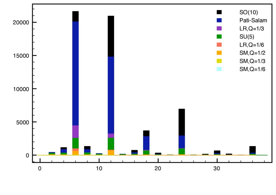
Figure 1: Distribution of the number of families for permutation orbifolds of standard Gepner Models.

Figure 1 shows the distribution of the number of families for permutation orbifolds of standard Gepner Models. All family numbers are even, as is the case for unpermuted Gepner models (we did not include exceptional MIPFs, which provides the only way to get three families in standard Gepner models). The greatest common denominator $\Delta$ of the number of families for a given tensor combination displays a similar behavior as observed in [22]. Two classes can be distinguished. Either $\Delta=6$ (or in a few cases a multiple of $6$), or $\Delta=2$ (sometimes 4), but there are no MIPFs with a number of families that is a multiple of three. In other words, the set of family numbers occurring in these two classes have no overlap whatsoever. It follows that in the second class there are no spectra with zero families. An interesting example is $(3,\langle 6,6\rangle,18)$. It has no spectra with chiral exotics, all spectra are chiral and have 4, 8, 16, 20, 28, 32, 40 or 56 families, of types $SO(10)$, Pati-Salam, $SU(5)\times U(1)$ or $SM,Q=1/2$. If we compare this with the unpermuted Gepner model we find some striking differences. In that case the same group types occur, but now there are spectra with chiral exotics, and the family quantization is in units of 2, not 4. In [22] an intriguing observation was made regarding the occurrence of these two classes. The second class was found to occur if all values $k_{i}$ of the factors in the tensor product are divisible by 3. This observation also holds for permutation orbifolds, if one uses the values of $k_{i}$ of the unpermuted theory.

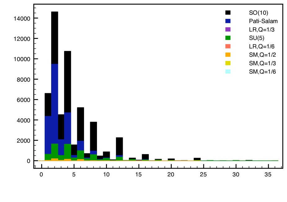
Figure 2: Distribution of the number of families for permutation orbifolds of lifted Gepner Models.

In figure 2 we show the family distribution for lifted Gepner models. As expected, this distribution looks a lot more favourable for three family models. The number three appears with more or less the same order of magnitude as two or four. However, there are some clear peaks at even family numbers, which were not visible in the analogous distribution for unpermuted Gepner models presented in [23]. For this reason three families are still suppressed by a factor of 3 to 4 with respect to 2 or 4 families, which is however a lot less than the two to three orders of magnitude observed in orientifold models [49].

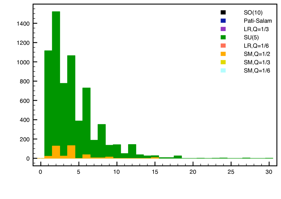
Figure 3: Distribution of the number of families for permutation orbifolds of B-L lifted (lift A) Gepner Models.

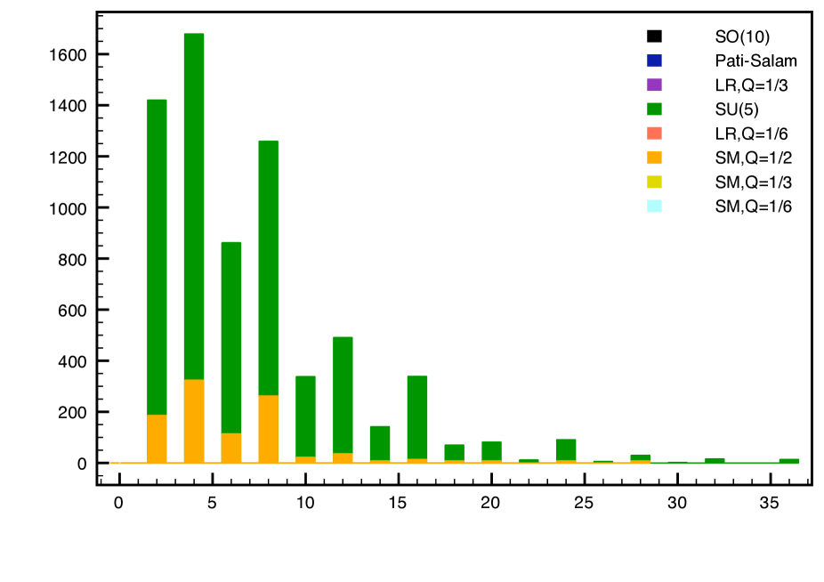
Figure 4: Distribution of the number of families for permutation orbifolds of B-L lifted (lift B) Gepner Models.

B-L lifts give similar results to those presented in [24]. Figure 3 contains the distribution of the number of families for permutation orbifolds of B-L lifted (lift A) Gepner models. Figure 4 contains the same, but for the lift B. Here, odd numbers are completely absent. Note that certain group types (namely those without a “$B-L$” type $U(1)$ factor) cannot occur in chiral spectra in these models, and that in the type that do occur the $U(1)$ is replaced by a non-abelian group.

8 Conclusions

In this paper we have considered $\mathbb{Z}_{2}$ permutation orbifolds of heterotic Gepner models. This should be viewed as an application of our previous paper [20] where $\mathbb{Z}_{2}$ permutations were studied for $N=2$ minimal models, which are the building blocks in Gepner construction.

Our main conclusion is that these new building blocks work as they should. They can be used on completely equal footing with all other available ones, which are the $N=2$ minimal models and some free-fermionic building blocks. We have checked the combination with minimal models and found full agreement with previous results on permutation orbifolds whenever they were available. The comparison did bring a few surprises, especially the fact that we were able to get new spectra for single permutations, where the old method of [7] gave nothing new.

We were able to go far beyond the old approach by finding many more $(2,2)$ models, as well as new $(0,2)$ models with $SO(10)$ breaking. We combined all this with heterotic weight lifting and B-L lifting. The main conclusion is that in most respects all observations concerning family number and fractional charges made for minimal models continue to hold in this new class. Also in this case weight lifting greatly enhances the set of three family models in comparison to neighboring numbers. Although this appears to give some entirely new models (Hodge number pairs that were not seen before), we found additional evidence for the observation of [7] that many of these models look like additional rational points in existing moduli spaces.

A next step in the exploration of these models is the study of couplings. An important problem to address is the possibility of lifting the vector-like states, especially the omnipresent fractionally charged ones, by giving vevs to moduli. In some cases, namely the permutation orbifolds with $k=2\mod 4$, one may run into the problem of unresolved fixed points for certain couplings. This problem did not arise here because we only studied spectra. But there are plenty of cases where this restriction does not apply. The fact that all building blocks with $k\not=\!2\mod 4$ are on equal footing with minimal models even with respect to fixed points should make it possible to develop an algorithm for determining couplings all at once for all cases. This is certainly a problem we intend to study in the near future.

Another application of our permutation orbifold CFTs could be to study the case of orientifold models. However, there we will face the same problem with fixed point resolution at an earlier stage, since the fixed point resolution matrices enter in the formula for boundary coefficients. We hope to address this issue in the future.

Appendix A Simple current invariants

Consider a simple current $J$ or order $N$, i.e. $J^{N}=1$. Define the monodromy parameter $r$ as

$$h_{J}=\frac{r(N-1)}{2N}\quad{\rm mod}\,\,\mathbb{Z}\,.$$ (A.1)

Also, define the monodromy charge $Q_{J}(\Phi)$ of $\Phi$ w.r.t. $J$ as

$$Q_{J}(\Phi)=h_{J}+h_{\Phi}-h_{J\phi}\quad{\rm mod}\,\,\mathbb{Z}\,.$$ (A.2)

The monodromy charge takes values $t/N$, with $t\in\mathbb{Z}$. The current $J$ organizes fields into orbits $(\Phi,J\Phi,\dots,J^{d}\Phi)$, where $d$ (not necessarily equal to $N$) is a divisor of $N$. On each orbit the monodromy charge is

$$Q_{J}(J^{n}\Phi)=\frac{t+rn}{N}\quad{\rm mod}\,\,\mathbb{Z}\,.$$ (A.3)

If a simple current $J$ exists in a (rational) CFT, and if it satisfies the condition that $N$ times its conformal weight is an integer, then it is known how to associate a modular invariant partition function to it. Suppose that the current $J$ has integer spin and order $N$. Then a MIPF is given by

$$Z(\tau,\bar{\tau})=\sum_{k,\,l}\bar{\chi}_{k}(\bar{\tau})M_{kl}(J)\chi_{l}(\tau)\,.$$ (A.4)

One way of expressing $M_{kl}(J)$ is [12, 13]:

$$M_{kl}(J)=\sum_{p=1}^{N}\delta(\Phi_{k},J^{p}\Phi_{l})\cdot\delta^{1}(\hat{Q}_{J}(\Phi_{k})+\hat{Q}_{J}(\Phi_{l}))\,$$ (A.5)

where $\delta^{1}(x)=1$ for $x=0$ mod $\mathbb{Z}$ and $\hat{Q}$ is defined on $J$-orbits as

$$\hat{Q}_{J}(J^{n}\Phi)=\frac{(t+rn)}{2N}\quad{\rm mod}\,\,\mathbb{Z}\,.$$ (A.6)

Morally speaking, $\hat{Q}$ is half the monodromy charge. Formula (A.5) defines a modular invariant partition functions, since it commutes with the $S$ and $T$ modular matrices, as shown in [9]. The set of all the simple currents forms an abelian group $\mathcal{G}$ under fusion multiplication. It is always a product of cyclic factors generated by a (conventionally chosen) complete subset of independent simple currents.

The foregoing associates a modular invariant partition function with a single simple current. One can construct even more of them by multiplying the matrices $M$. The most general simple current MIPF associated with a given subgroup of $\mathcal{G}$ can be obtained as follows [12, 22]. Choose a subgroup of $\mathcal{G}$ denoted $\mathcal{H}$, such that each element satisfies the effective center condition $Nh_{J}\in\mathbb{Z}$. Its generators are simple currents $J_{s}$, $s=1,\dots,k$ for some $k$. They have relative monodromies $Q_{J_{s}}(J_{t})=R_{st}$. Take any matrix $X$ that satisfies the equation

$$X+X^{T}=R\,.$$ (A.7)

The matrix $X$ (called the torsion matrix) determines the multiplicities $M_{ij}$ according to

$$M_{ij}(\mathcal{H},X)={\rm nr.\,\,of\,\,solutions}\,\,K\,\,{\rm to\,\,the\,\,conditions:}$$ (A.8)

• $j=Ki$, $K\in\mathcal{H}$.

• $Q_{M}(i)+X(M,K)=0$ mod 1 for all $M\in\mathcal{H}$ .

Here $X(K,J)$ is defined in terms of the generating current $J_{s}$ as

$$X(K,J)\equiv\sum_{s,t}n_{s}m_{t}X_{st}\,,$$ (A.9)

with $K=(J_{1})^{n_{1}}\dots(J_{k})^{n_{k}}$ and $J=(J_{1})^{m_{1}}\dots(J_{k})^{m_{k}}$.

A.1 A small theorem

In this subsection we prove the following theorem.

Theorem A.1.

The following statements are true.
i) If a simple current $J$ is local w.r.t. any other current $K$, i.e. $Q_{K}(J)=0$ (mod $\mathbb{Z}$), then $M_{JJ}(K)\neq 0$.
ii) For a simple current $J$, which is local w.r.t. any other current $K$, $M_{J0}(K)=M_{0J}(K)$. In particular, if $M_{J0}(K)\neq 0$, then also $M_{0J}(K)\neq 0$.

Proof.

For the proof we use the statement (A.8).
Let us start with i) and consider $M_{JJ}(K,X)$. The first condition in (A.8) has only one solution, namely $K=0$. The second condition reads

$$Q_{M}(J)+X(M,0)=0\qquad\forall M$$ (A.10)

and is always true, because the two terms vanish separately. This proves that $M_{JJ}(K)\neq 0$.

Point ii) goes as follows. Consider $M_{0J^{c}}(K,X)$. There is again only one solution to the first condition, namely $K=J^{c}$. The second condition reads

$$Q_{M}(0)+X(M,J^{c})=0\,.$$ (A.11)

The first term vanishes by hypothesis, while the second is either zero (in which case $M_{0J^{c}}(K,X)\neq 0$) or non-zero (in which case $M_{0J^{c}}(K,X)=0$).
Similarly, look at $M_{J0}(K,X)$. There is again only one solution to the first condition, namely $K=J^{c}$. The second condition reads

$$Q_{M}(0)+X(M,J^{c})=0\,.$$ (A.12)

The first term vanishes by hypothesis, while the second is either zero or non-zero. In any case, the same condition holds for both $M_{0J^{c}}(K,X)$ and $M_{J0}(K,X)$. This implies that $M_{J0}(K,X)=M_{0J^{c}}(K,X)$ (note that these matrix elements can only be 0 or 1). By closure of the algebra, and because $J^{c}$ is always a power of $J$, we may replace $J^{c}$ by $J$ in this relation. ∎

Consider now the permutation orbifold. This theorem applies in particular to the un-orbifold current $J=(0,1)$ when coupled to any other current $K$, which is either a standard (diagonal) or an exceptional (off-diagonal) one. In fact, using the same procedure as we did in [17] to compute the simple current and fixed point structure of the permutation orbifold, one can show that

$$N_{(J,\psi)\langle pq\rangle}^{\phantom{(J,\psi)\langle pq\rangle}\langle p^{\prime}q^{\prime}\rangle} = N_{Jp}^{\phantom{Jp}p^{\prime}}N_{Jq}^{\phantom{Jq}q^{\prime}}+N_{Jp}^{\phantom{Jp}q^{\prime}}N_{Jq}^{\phantom{Jq}p^{\prime}}\,,$$

$$N_{(J,\psi)(i,\chi)}^{\phantom{(J,\psi)(i,\chi)}(i^{\prime},\chi^{\prime})} = \frac{1}{2}N_{Ji}^{\phantom{Ji}i^{\prime}}(N_{Ji}^{\phantom{Ji}i^{\prime}}+e^{i\pi(\psi+\chi-\chi^{\prime})})\,.$$

Hence, for the current $(J,\psi)=(0,1)$, we have

$$N_{(0,1)\langle pq\rangle}^{\phantom{(0,1)\langle pq\rangle}\langle p^{\prime}q^{\prime}\rangle}=\delta_{p}^{p^{\prime}}\delta_{q}^{q^{\prime}}+\delta_{p}^{q^{\prime}}\delta_{q}^{p^{\prime}}=\delta_{p}^{p^{\prime}}\delta_{q}^{q^{\prime}}\,,$$

namely $\langle pq\rangle$ must be fixed by $(0,1)$ in order for this to be non-zero (recall that $p<q$ and $p^{\prime}<q^{\prime}$), and

$$N_{(0,1)(i,\chi)}^{\phantom{(0,1)(i,\chi)}(i^{\prime},\chi^{\prime})}=\frac{1}{2}\delta_{i}^{i^{\prime}}(\delta_{i}^{i^{\prime}}-e^{i\pi(\chi-\chi^{\prime})})\,$$

which is non-zero only if $i=i^{\prime}$ and $\chi\neq\chi^{\prime}$ (recall that we can think of $\chi$ as defined mod $2$). Equivalently, in the fusion language:

$$(0,1)\cdot\langle pq\rangle=\langle pq\rangle\quad,\qquad(0,1)\cdot(i,\chi)=(i,\chi+1)\,.$$ (A.13)

This implies that $(0,1)$ has zero monodromy charge w.r.t. any other current, since

$$Q_{\langle pq\rangle}\big{(}(0,1)\big{)} = h_{\langle pq\rangle}+h_{(0,1)}-h_{\langle pq\rangle}=0\quad{\rm mod}\,\,\mathbb{Z}\,,$$

$$Q_{(i,\chi)}\big{(}(0,1)\big{)} = h_{(i,\chi)}+h_{(0,1)}-h_{(i,\chi+1)}=0\quad{\rm mod}\,\,\mathbb{Z}\,.$$

Now, the un-orbifold current $(0,1)$ has order two, hence $J^{c}=J$ and $M_{J0}(K,X)=M_{0J}(K,X)$. This also implies that its existence on left-moving sector is guaranteed by its existence on the right-moving sector (and vice-versa).

A.2 Summary of results

Here we present four tables summarizing the results on the number of families for the standard, heterotic weight lifted, B-L lifted (lift A) and B-L lifted (lift B) cases. These tables contain information about spectra in which the un-orbifold current is not allowed in the chiral algebra. This means that these are genuine permutation orbifold spectra. By inspection, we do indeed find that these spectra are usually different than those obtained in the unpermuted case. In the columns we specify respectively the tensor combination the greatest common divisor $\Delta$ of the number of families for all MIPFs of the tensor product and the maximal net number of families encountered. In the next column we indicate which of the seven $SO(10)$ subgroups occur, with the labelling

• 0: SM, Q=1/6

• 1: SM, Q=1/3

• 2: SM, Q=1/2

• 3: LR, Q=1/6

• 4: $SU(5)\times U(1)$

• 5: LR, Q=1/3

• 6: Pati-Salam.

Since $SO(10)$ can always occur there is no need to indicate it. In [22] a simple criterion was derived to determine which subgroups can occur in each standard Gepner model. The allowed subgroups for permutation orbifolds of Gepner models are a subset of these. In some cases, such as $(\langle 5,5\rangle,5,12)$ some of the subgroups cannot be realized. In the column labelled “Exotics” we indicate if, for a given tensor product, spectra with chiral exotics occur. Note that in most cases the absence of such spectra is a consequence of the fact that only GUT gauge groups occur. In the next columns we list the number of distinct three family and in column 6 the number of distinct $N$-family $(N>0)$ spectra. In these tables only cases with $\Delta>0$ are shown. If a permutation orbifold seems to be missing, than either it is a permutation for $k>10$, or it is a purely odd tensor product for which all permutations are trivial, or it has only non-chiral spectra and hence $\Delta=0$ and there are no chiral exotics. In column 1 of the second table, $\langle\cal{A},\cal{A}\rangle$ denotes the permutation orbifold of CFT ${\cal A}$, a hat indicates the lifted CFT, and a tilde indicates the second lift of a CFT. It turns out that in the only permutation orbifold with two distinct lifts of the same factor, $(\hat{5},\langle 5,5\rangle,12)$ and $(\tilde{5},\langle 5,5\rangle,12)$, $\Delta=0$ in both cases, which is why a tilde never occurs in the tables. The last column indicates which percentage of the spectra has no mirror. Since mirror symmetry is exact in the full set, this gives an indication of how close our random scan is to a full enumeration.

Table 4: Results for standard Gepner models

model	$\Delta$	Max.	Groups	Exotics	3 family	$N$ fam.	Missing
$(1,1,1,1,1,\langle 4,4\rangle)$	6	84	3,5,6	Yes	0	342	6.14%
$(1,1,1,1,\langle 10,10\rangle)$	6	48	3,5,6	Yes	0	124	4.84%
$(1,1,1,1,\langle 2,2\rangle,4)$	6	48	3,5,6	Yes	0	75	6.67%
$(1,1,1,\langle 4,4\rangle,4)$	6	84	3,5,6	Yes	0	2717	22.89%
$(1,1,2,2,\langle 4,4\rangle)$	6	24	3,5,6	Yes	0	106	0.00%
$(1,1,\langle 2,2\rangle,2,10)$	6	48	3,5,6	Yes	0	662	7.70%
$(1,1,4,\langle 10,10\rangle)$	6	72	3,5,6	Yes	0	493	7.10%
$(1,1,\langle 6,6\rangle,10)$	12	24	3,5,6	Yes	0	63	0.00%
$(1,1,\langle 2,2\rangle,4,4)$	6	48	3,5,6	Yes	0	226	6.19%
$(1,1,\langle 2,2\rangle,\langle 4,4\rangle)$	12	24	3,5,6	Yes	0	73	6.85%
$(1,2,2,\langle 10,10\rangle)$	6	60	3,5,6	Yes	0	191	4.71%
$(1,\langle 2,2\rangle,2,2,4)$	12	60	3,5,6	Yes	0	363	3.31%
$(1,2,4,\langle 6,6\rangle)$	12	48	3,5,6	Yes	0	57	3.51%
$(1,2,\langle 4,4\rangle,10)$	6	60	3,5,6	Yes	0	1605	14.08%
$(1,2,\langle 3,3\rangle,58)$	6	24	0,1,2,3,4,5,6	Yes	0	102	0.00%
$(1,\langle 4,4\rangle,4,4)$	6	84	3,5,6	Yes	0	5605	6.57%
$(1,\langle 2,2\rangle,10,10)$	6	84	3,5,6	Yes	0	989	6.47%
$(1,\langle 3,3\rangle,4,8)$	6	36	0,1,2,3,4,5,6	Yes	0	37	0.00%
$(1,\langle 2,2\rangle,6,22)$	6	60	3,5,6	Yes	0	985	3.25%
$(1,\langle 2,2\rangle,7,16)$	12	48	3,5,6	Yes	0	41	0.00%
$(1,\langle 2,2\rangle,\langle 2,2\rangle,4)$	12	60	3,5,6	Yes	0	165	0.61%
$(\langle 2,2\rangle,2,2,2,2)$	6	90	6	Yes	0	1849	5.19%
$(2,2,2,\langle 6,6\rangle)$	12	72	6	Yes	0	245	0.00%
$(2,2,\langle 4,4\rangle,4)$	6	48	3,5,6	Yes	0	250	0.00%
$(2,2,\langle 3,3\rangle,8)$	6	36	2,4,6	Yes	0	55	0.00%
$(2,2,\langle 2,2\rangle,\langle 2,2\rangle)$	6	90	6	Yes	0	1580	1.58%
$(2,\langle 10,10\rangle,10)$	6	102	3,5,6	Yes	0	328	0.00%
$(2,\langle 8,8\rangle,18)$	6	72	2,4,6	Yes	0	316	0.00%
$(\langle 2,2\rangle,2,3,18)$	6	60	2,4,6	Yes	0	780	4.36%
$(2,\langle 7,7\rangle,34)$	12	48	3,5,6	Yes	0	9	0.00%
$(\langle 2,2\rangle,2,4,10)$	6	66	3,5,6	Yes	0	1550	3.81%
$(\langle 2,2\rangle,2,6,6)$	6	84	6	Yes	0	1735	3.80%
$(2,\langle 2,2\rangle,\langle 6,6\rangle)$	12	72	$SO(10)$ only	No	0	219	0.00%
$(3,\langle 6,6\rangle,18)$	4	56	2,4,6	No	0	232	0.00%
$(3,\langle 5,5\rangle,68)$	24	24	4	No	0	18	0.00%
$(3,\langle 8,8\rangle,8)$	6	96	2,4,6	Yes	0	1909	1.41%
$(3,\langle 3,3\rangle,\langle 3,3\rangle)$	2	56	4	No	0	126	0.00%
$(4,4,\langle 10,10\rangle)$	6	90	5	Yes	0	188	0.00%
$(4,\langle 6,6\rangle,10)$	12	48	5	Yes	0	70	0.00%
$(4,\langle 5,5\rangle,19)$	12	24	5	Yes	0	6	0.00%
$(4,\langle 7,7\rangle,7)$	12	60	5	Yes	0	11	0.00%
$(\langle 5,5\rangle,5,12)$	6	78	$SO(10)$ only	No	0	44	0.00%
$(\langle 6,6\rangle,6,6)$	2	104	6	Yes	0	1230	0.00%
$(\langle 4,4\rangle,10,10)$	6	96	3,5,6	Yes	0	693	0.72%
$(\langle 3,3\rangle,10,58)$	6	60	0,1,2,3,4,5,6	Yes	0	97	0.00%
$(\langle 3,3\rangle,12,33)$	2	20	4	No	0	30	0.00%
$(\langle 3,3\rangle,13,28)$	6	84	1,4,5	Yes	0	587	0.00%
$(\langle 3,3\rangle,18,18)$	2	116	2,4,6	Yes	0	681	0.00%
$(\langle 2,2\rangle,3,3,8)$	6	48	2,4,6	Yes	0	332	3.61%
$(\langle 2,2\rangle,4,4,4)$	6	54	5	Yes	0	75	0.00%
$(\langle 4,4\rangle,5,40)$	6	48	3,5,6	Yes	0	98	0.00%
$(\langle 4,4\rangle,6,22)$	6	60	3,5,6	Yes	0	440	0.00%
$(\langle 4,4\rangle,7,16)$	6	72	3,5,6	Yes	0	271	0.00%
$(\langle 4,4\rangle,8,13)$	6	48	0,1,2,3,4,5,6	Yes	0	180	0.00%
$(\langle 3,3\rangle,9,108)$	2	28	4	No	0	30	0.00%
$(\langle 6,6\rangle,\langle 6,6\rangle)$	4	80	$SO(10)$ only	No	0	152	0.00%
$(\langle 2,2\rangle,\langle 4,4\rangle,4)$	6	48	5	Yes	0	103	0.00%
$(\langle 2,2\rangle,\langle 3,3\rangle,8)$	6	36	4	No	0	37	0.00%
$(\langle 2,2\rangle,\langle 2,2\rangle,\langle 2,2\rangle)$	6	90	$SO(10)$ only	No	0	224	1.34%
$(1,\langle 2,2\rangle,\langle 10,10\rangle)$	12	60	3,5,6	Yes	0	155	0.00%
$(\langle 4,4\rangle,\langle 10,10\rangle)$	6	72	5	Yes	0	142	0.00%
$(1,\langle 4,4\rangle,\langle 4,4\rangle)$	6	84	3,5,6	Yes	0	848	0.83%

Table 5: Results for lifted Gepner models

model	$\Delta$	Max.	Groups	Exotics	3 family	$N$ fam.	Missing
$(\widehat{1},1,1,1,1,\langle 4,4\rangle)$	3	33	3,5,6	Yes	45	205	16.10%
$(\widehat{1},1,1,1,\langle 10,10\rangle)$	3	24	3,5,6	Yes	0	39	2.56%
$(\widehat{1},1,1,1,\langle 2,2\rangle,4)$	3	18	3,5,6	Yes	16	50	14.00%
$(\widehat{1},1,1,\langle 4,4\rangle,4)$	3	33	3,5,6	Yes	549	1016	28.54%
$(\widehat{1},1,2,2,\langle 4,4\rangle)$	3	12	3,5,6	Yes	17	60	0.00%
$(\widehat{1},1,\langle 2,2\rangle,2,10)$	3	24	3,5,6	Yes	123	283	7.42%
$(\widehat{1},1,4,\langle 10,10\rangle)$	3	24	3,5,6	Yes	33	206	7.77%
$(\widehat{1},1,\langle 6,6\rangle,10)$	6	6	3,5,6	Yes	0	15	0.00%
$(\widehat{1},1,\langle 2,2\rangle,4,4)$	3	24	3,5,6	Yes	34	237	4.64%
$(\widehat{1},1,\langle 2,2\rangle,\langle 4,4\rangle)$	6	12	3,5,6	Yes	0	38	0.00%
$(\widehat{1},2,2,\langle 10,10\rangle)$	12	24	3,5,6	Yes	0	18	0.00%
$(\widehat{1},\langle 2,2\rangle,2,2,4)$	6	24	3,5,6	Yes	0	71	7.04%
$(\widehat{1},2,\langle 3,3\rangle,58)$	1	8	0,1,2,3,4,5,6	Yes	2	40	0.00%
$(\widehat{1},\langle 2,2\rangle,10,10)$	6	24	3,5,6	Yes	0	105	5.71%
$(\widehat{1},\langle 3,3\rangle,4,8)$	2	8	0,1,2,3,4,5,6	Yes	0	23	0.00%
$(\widehat{1},\langle 2,2\rangle,6,22)$	3	24	3,5,6	Yes	58	281	5.69%
$(\widehat{1},\langle 2,2\rangle,7,16)$	6	12	3,5,6	Yes	0	13	0.00%
$(\widehat{2},\langle 2,2\rangle,2,2,2)$	1	36	6	Yes	587	10481	6.91%
$(\widehat{2},2,2,\langle 6,6\rangle)$	2	36	6	Yes	0	595	0.17%
$(\widehat{2},2,\langle 3,3\rangle,8)$	1	10	2,4,6	Yes	3	51	0.00%
$(\widehat{2},2,\langle 2,2\rangle,\langle 2,2\rangle)$	2	24	6	Yes	0	807	1.73%
$(\widehat{2},\langle 10,10\rangle,10)$	4	8	3,5,6	Yes	0	24	0.00%
$(\widehat{2},\langle 8,8\rangle,18)$	1	12	2,4,6	Yes	6	85	0.00%
$(\widehat{2},\langle 2,2\rangle,3,18)$	1	24	2,4,6	Yes	26	225	4.00%
$(\widehat{2},\langle 2,2\rangle,4,10)$	2	24	3,5,6	Yes	0	89	3.37%
$(\widehat{2},\langle 2,2\rangle,6,6)$	1	24	6	Yes	9	305	1.97%
$(\widehat{3},\langle 6,6\rangle,18)$	2	20	2,4,6	No	0	85	0.00%
$(\widehat{3},\langle 5,5\rangle,68)$	12	12	4	No	0	4	0.00%
$(\widehat{3},\langle 8,8\rangle,8)$	1	48	2,4,6	Yes	146	1709	0.06%
$(\widehat{3},\langle 3,3\rangle,\langle 3,3\rangle)$	1	28	4	No	11	80	0.00%
$(\widehat{4},4,\langle 10,10\rangle)$	2	16	5	Yes	0	47	0.00%
$(\widehat{4},\langle 7,7\rangle,7)$	1	3	5	Yes	2	6	0.00%
$(\widehat{6},\langle 6,6\rangle,6)$	1	8	6	Yes	7	85	0.00%
$(\langle 3,3\rangle,10,\widehat{58})$	1	6	0,1,2,3,4,5,6	Yes	2	11	0.00%
$(\langle 3,3\rangle,\widehat{12},33)$	2	6	4	No	0	5	0.00%
$(\langle 3,3\rangle,\widehat{13},28)$	1	30	1,4,5	Yes	29	170	0.00%
$(\langle 2,2\rangle,\widehat{3},3,8)$	1	24	2,4,6	Yes	14	479	4.38%
$(\langle 2,2\rangle,\widehat{4},4,4)$	2	24	5	Yes	0	111	0.90%
$(\langle 4,4\rangle,\widehat{6},22)$	8	8	3,5,6	Yes	0	5	0.00%
$(\langle 4,4\rangle,\widehat{8},13)$	4	16	0,1,2,3,4,5,6	Yes	0	17	0.00%
$(\langle 3,3\rangle,\widehat{9},108)$	2	6	4	No	0	6	0.00%
$(\widehat{4},\langle 2,2\rangle,\langle 4,4\rangle)$	4	20	5	Yes	0	53	0.00%
$(\langle 2,2\rangle,\langle 3,3\rangle,\widehat{8})$	2	6	4	No	0	11	0.00%
$(1,1,1,\widehat{4},\langle 4,4\rangle)$	1	24	3,5,6	Yes	78	859	20.84%
$(1,1,\widehat{2},2,\langle 4,4\rangle)$	1	6	3,5,6	Yes	0	75	4.00%
$(1,1,\widehat{2},\langle 2,2\rangle,10)$	1	24	3,5,6	Yes	20	323	8.05%
$(1,1,\widehat{4},\langle 10,10\rangle)$	2	16	3,5,6	Yes	0	191	4.71%
$(1,1,\langle 2,2\rangle,\widehat{4},4)$	2	32	3,5,6	Yes	0	297	5.05%
$(1,\widehat{2},2,\langle 10,10\rangle)$	1	16	3,5,6	Yes	28	262	0.00%
$(1,\langle 2,2\rangle,2,2,\widehat{4})$	4	32	3,5,6	Yes	0	118	8.47%
$(1,\widehat{2},4,\langle 6,6\rangle)$	2	24	3,5,6	Yes	0	77	0.00%
$(1,\widehat{2},\langle 4,4\rangle,10)$	1	16	3,5,6	Yes	147	1160	8.71%
$(1,\widehat{2},\langle 3,3\rangle,58)$	1	8	0,1,2,3,4,5,6	Yes	3	56	0.00%
$(1,\widehat{4},\langle 4,4\rangle,4)$	1	24	3,5,6	Yes	425	3219	6.28%
$(1,\langle 3,3\rangle,\widehat{4},8)$	2	10	0,1,2,3,4,5,6	Yes	0	27	0.00%
$(1,\langle 2,2\rangle,\widehat{6},22)$	1	48	3,5,6	Yes	46	645	3.41%
$(2,2,\widehat{4},\langle 4,4\rangle)$	4	20	3,5,6	Yes	0	93	0.00%
$(2,2,\langle 3,3\rangle,\widehat{8})$	2	8	2,4,6	Yes	0	29	0.00%
$(\langle 2,2\rangle,2,\widehat{3},18)$	2	30	2,4,6	Yes	0	380	2.63%
$(\langle 2,2\rangle,2,\widehat{4},10)$	4	24	3,5,6	Yes	0	107	0.93%
$(\langle 2,2\rangle,2,\widehat{6},6)$	2	48	6	Yes	0	477	2.73%
$(3,\widehat{8},\langle 8,8\rangle)$	1	32	2,4,6	Yes	24	480	0.00%
$(\langle 5,5\rangle,5,\widehat{12})$	1	6	$SO(10)$ only	No	2	8	0.00%
$(\langle 2,2\rangle,3,3,\widehat{8})$	1	18	2,4,6	Yes	6	116	0.00%
$(\langle 4,4\rangle,8,\widehat{13})$	2	14	0,1,2,3,4,5,6	Yes	0	20	0.00%
$(1,\widehat{2},\langle 2,2\rangle,2,4)$	2	24	3,5,6	Yes	0	1092	4.85%
$(1,2,\langle 3,3\rangle,\widehat{58})$	2	12	0,1,2,3,4,5,6	Yes	0	11	0.00%
$(1,\langle 3,3\rangle,4,\widehat{8})$	2	6	0,1,2,3,4,5,6	Yes	0	10	0.00%

Table 6: Results for B-L lifted (lift A) Gepner models

model	$\Delta$	Max.	Groups	Exotics	3 family	$N$ fam.	Missing
$(1,2,\langle 3,3\rangle,58)$	1	6	0,1,2,3,4,5,6	Yes	4	33	0.00%
$(1,\langle 3,3\rangle,4,8)$	2	6	0,1,2,3,4,5,6	Yes	0	12	0.00%
$(2,2,\langle 3,3\rangle,8)$	2	8	2,4,6	Yes	0	25	0.00%
$(2,\langle 8,8\rangle,18)$	1	12	2,4,6	Yes	14	90	0.00%
$(\langle 2,2\rangle,2,3,18)$	2	18	2,4,6	Yes	0	364	3.85%
$(3,\langle 6,6\rangle,18)$	2	14	2,4,6	No	0	84	0.00%
$(3,\langle 5,5\rangle,68)$	6	6	4	No	0	12	0.00%
$(3,\langle 8,8\rangle,8)$	1	30	2,4,6	Yes	238	1799	0.11%
$(3,\langle 3,3\rangle,\langle 3,3\rangle)$	1	18	4	No	15	84	0.00%
$(\langle 3,3\rangle,10,58)$	1	10	0,1,2,3,4,5,6	Yes	1	19	0.00%
$(\langle 3,3\rangle,12,33)$	2	4	4	No	0	6	0.00%
$(\langle 3,3\rangle,13,28)$	1	9	1,4,5	Yes	57	346	0.00%
$(\langle 3,3\rangle,18,18)$	1	14	2,4,6	Yes	30	200	0.00%
$(\langle 2,2\rangle,3,3,8)$	1	12	2,4,6	Yes	30	246	0.00%
$(\langle 4,4\rangle,8,13)$	2	8	0,1,2,3,4,5,6	Yes	0	49	0.00%
$(\langle 3,3\rangle,9,108)$	2	4	4	No	0	6	0.00%
$(\langle 2,2\rangle,\langle 3,3\rangle,8)$	2	6	4	No	0	12	0.00%

Table 7: Results for B-L lifted Gepner (lift B) models

model	$\Delta$	Max.	Groups	Exotics	3 family	$N$ fam.	Missing
$(1,2,\langle 3,3\rangle,58)$	2	10	0,1,2,3,4,5,6	Yes	0	32	0.00%
$(1,\langle 3,3\rangle,4,8)$	2	10	0,1,2,3,4,5,6	Yes	0	10	0.00%
$(2,2,\langle 3,3\rangle,8)$	2	14	2,4,6	Yes	0	34	0.00%
$(2,\langle 8,8\rangle,18)$	2	16	2,4,6	Yes	0	108	0.00%
$(\langle 2,2\rangle,2,3,18)$	2	36	2,4,6	Yes	0	476	3.99%
$(3,\langle 6,6\rangle,18)$	4	28	2,4,6	No	0	82	0.00%
$(3,\langle 5,5\rangle,68)$	8	16	4	No	0	12	0.00%
$(3,\langle 8,8\rangle,8)$	2	56	2,4,6	Yes	0	1781	0.00%
$(3,\langle 3,3\rangle,\langle 3,3\rangle)$	2	32	4	No	0	81	0.00%
$(\langle 3,3\rangle,10,58)$	2	18	0,1,2,3,4,5,6	Yes	0	18	0.00%
$(\langle 3,3\rangle,12,33)$	2	8	4	No	0	6	0.00%
$(\langle 3,3\rangle,13,28)$	2	18	1,4,5	Yes	0	322	0.00%
$(\langle 3,3\rangle,18,18)$	2	26	2,4,6	Yes	0	191	0.00%
$(\langle 2,2\rangle,3,3,8)$	2	24	2,4,6	Yes	0	226	0.00%
$(\langle 4,4\rangle,8,13)$	4	16	0,1,2,3,4,5,6	Yes	0	45	0.00%
$(\langle 3,3\rangle,9,108)$	2	10	4	No	0	6	0.00%
$(\langle 2,2\rangle,\langle 3,3\rangle,8)$	2	10	4	No	0	10	0.00%

References

- [1] D. J. Gross, J. A. Harvey, E. J. Martinec, R. Rohm, “The Heterotic String”, Phys. Rev. Lett. 54 (1985) 502-505.
- [2] A. A. Belavin, A. M. Polyakov and A. B. Zamolodchikov, “Infinite conformal symmetry in two-dimensional quantum field theory,” Nucl. Phys. B 241 (1984) 333.
- [3] D. Gepner, “Space-Time Supersymmetry in Compactified String Theory and Superconformal Models,” Nucl. Phys. B 296 (1988) 757.
- [4] D. Gepner, “Exactly Solvable String Compactifications on Manifolds of SU(N) Holonomy,” Phys. Lett. B 199 (1987) 380.
- [5] Y. Kazama and H. Suzuki, “New N=2 Superconformal Field Theories and Superstring Compactification,” Nucl. Phys. B 321 (1989) 232.
- [6] A. Klemm and M. G. Schmidt, “Orbifolds by cyclic permutations of tensor product conformal field theories,” Phys. Lett. B 245 (1990) 53.
- [7] J. Fuchs, A. Klemm and M. G. Schmidt, “Orbifolds by cyclic permutations in Gepner type superstrings and in the corresponding Calabi-Yau manifolds,” Annals Phys. 214 (1992) 221.
- [8] A. N. Schellekens and S. Yankielowicz, “Extended Chiral Algebras and Modular Invariant Partition Functions” Nucl. Phys. B 327 (1989) 673.
- [9] A. N. Schellekens and S. Yankielowicz, “Modular invariants from simple currents: an explicit proof,” Phys. Lett. B 227 (1989) 387.
- [10] K. A. Intriligator, “Bonus Symmetry in Conformal Field Theory” Nucl. Phys. B 332 (1990) 541.
- [11] B. Gato-Rivera and A. N. Schellekens, “Complete classification of simple current modular invariants for (Z(p))**k”, Commun. Math. Phys. 145 (1992) 85.
- [12] M. Kreuzer and A. N. Schellekens, “Simple currents versus orbifolds with discrete torsion: A Complete classification,” Nucl. Phys. B 411 (1994) 97 [arXiv:hep-th/9306145].
- [13] A. N. Schellekens and S. Yankielowicz, “New Modular Invariants for N=2 Tensor Products and Four-Dimensional Strings,” Nucl. Phys. B 330 (1990) 103.
- [14] A. Font, L. E. Ibanez, F. Quevedo, “String Compactifications And N=2 Superconformal Coset Constructions,” Phys. Lett. B224 (1989) 79.
- [15] A. N. Schellekens, “Field identification fixed points in N=2 coset theories,” Nucl. Phys. B 366 (1991) 27.
- [16] L. Borisov, M. B. Halpern and C. Schweigert, “Systematic approach to cyclic orbifolds,” Int. J. Mod. Phys. A 13 (1998) 125 [arXiv:hep-th/9701061].
- [17] M. Maio and A. N. Schellekens, “Fixed Point Resolution in Extensions of Permutation Orbifolds,” Nucl. Phys. B 821 (2009) 577 [arXiv:0905.1632 [hep-th]].
- [18] M. Maio and A. N. Schellekens, “Complete Analysis of Extensions of Permutation Orbifolds,” arXiv:0907.3053 [hep-th].
- [19] M. Maio and A. N. Schellekens, “Formula for Fixed Point Resolution Matrix of Permutation Orbifolds,” Nucl. Phys. B 830 (2010) 116 [arXiv:0911.1901 [hep-th]].
- [20] M. Maio and A. N. Schellekens, “Permutation Orbifold of N=2 Supersymmetric Minimal Models,” arXiv:1011.0934 [hep-th].
- [21] B. Gato-Rivera and A. N. Schellekens, “Heterotic Weight Lifting,” Nucl. Phys. B 828 (2010) 375 [arXiv:0910.1526 [hep-th]].
- [22] B. Gato-Rivera and A. N. Schellekens, “Asymmetric Gepner Models (Revisited),” Nucl. Phys. B 841 (2010) 100 [arXiv:1003.6075 [hep-th]].
- [23] B. Gato-Rivera, A. N. Schellekens and A. N. Schellekens, “Asymmetric Gepner Models II. Heterotic Weight Lifting,” arXiv:1009.1320 [hep-th].
- [24] B. Gato-Rivera and A. N. Schellekens, “Asymmetric Gepner Models III. B-L Lifting,” arXiv:1012.0796 [hep-th].
- [25] B. Gato-Rivera, A. N. Schellekens, “Asymmetric Gepner Models IV. E8 breaking,” (to appear).
- [26] A. N. Schellekens and S. Yankielowicz, “Field identification fixed points in the coset construction,” Nucl. Phys. B 334 (1990) 67.
- [27] A. N. Schellekens and S. Yankielowicz, “Simple currents, modular invariants and fixed points,” Int. J. Mod. Phys. A 5 (1990) 2903.
- [28] J. Fuchs, A. N. Schellekens and C. Schweigert, “A matrix S for all simple current extensions,” Nucl. Phys. B 473 (1996) 323 [arXiv:hep-th/9601078].
- [29] J. Fuchs, B. Schellekens and C. Schweigert, “From Dynkin diagram symmetries to fixed point structures,” Commun. Math. Phys. 180 (1996) 39 [arXiv:hep-th/9506135].
- [30] A. N. Schellekens, “Fixed point resolution in extended WZW-models,” Nucl. Phys. B 558 (1999) 484 [arXiv:math/9905153].
- [31] J. Fuchs, B. Schellekens, C. Schweigert, “The resolution of field identification fixed points in diagonal coset theories,” Nucl. Phys. B461 (1996) 371-406. [hep-th/9509105].
- [32] G. Pradisi, A. Sagnotti, Y. .S. Stanev, “Completeness conditions for boundary operators in 2-D conformal field theory”, Phys. Lett. B381 (1996) 97-104. [hep-th/9603097].
- [33] G. Pradisi, A. Sagnotti, Y. .S. Stanev, “The Open descendants of nondiagonal SU(2) WZW models”, Phys. Lett. B356 (1995) 230-238. [hep-th/9506014].
- [34] J. Fuchs, L. R. Huiszoon, A. N. Schellekens, C. Schweigert, J. Walcher, “Boundaries, crosscaps and simple currents”, Phys. Lett. B495 (2000) 427-434. [hep-th/0007174].
- [35] W. Lerche, D. Lüst and A. N. Schellekens, “Chiral Four-Dimensional Heterotic Strings From Selfdual Lattices”, Nucl. Phys. B 287 (1987) 477.
- [36] D. Gepner, “String Theory On Calabi-Yau Manifolds: The Three Generations Case”, arXiv:hep-th/9301089.
- [37] www.nikhef.nl/t58, page “Hodge numbers”
- [38] A. N. Schellekens, “Electric charge quantization in String Theory”, Phys. Lett. B 237 (1990) 363.
- [39] X. G. Wen and E. Witten, “Electric And Magnetic Charges In Superstring Models”, Nucl. Phys. B 261 (1985) 651.
- [40] G. G. Athanasiu, J. J. Atick, M. Dine and W. Fischler, “Remarks on Wilson line, Modular Invariance and Possible String Relics in Calabi-Yau Compactifications”, Phys. Lett. B 214 (1988) 55.
- [41] M. L. Perl, E. R. Lee and D. Loomba, “Searches For Fractionally Charged Particles”, Ann. Rev. Nucl. Part. Sci. 59 (2009) 47.
-
[42]
B. Assel, K. Christodoulides, A. E. Faraggi, C. Kounnas and J. Rizos,
“Exophobic Quasi-Realistic Heterotic String Vacua,”
Phys. Lett. B 683, 306 (2010)
[arXiv:0910.3697 [hep-th]].
J. Rizos, “The ’landscape’ of Pati–Salam heterotic superstring vacua,” arXiv:1003.0458 [hep-th].
B. Assel, K. Christodoulides, A. E. Faraggi, C. Kounnas and J. Rizos, “Classification of Heterotic Pati-Salam Models,” arXiv:1007.2268 [hep-th]. - [43] E. Witten, “Symmetry Breaking Patterns in Superstring Models”, Nucl. Phys. B258 (1985) 75.
- [44] M. Blaszczyk, S. G. Nibbelink, M. Ratz, F. Ruehle, M. Trapletti, P. K. S. Vaudrevange, “A Z2xZ2 standard model”, Phys. Lett. B683 (2010) 340-348. [arXiv:0911.4905 [hep-th]].
- [45] W. Buchmuller, K. Hamaguchi, O. Lebedev and M. Ratz, “Supersymmetric standard model from the heterotic string”, Phys. Rev. Lett. 96 (2006) 121602 [arXiv:hep-ph/0511035].
- [46] O. Lebedev, H. P. Nilles, S. Raby, S. Ramos-Sanchez, M. Ratz, P. K. S. Vaudrevange and A. Wingerter, “A mini-landscape of exact MSSM spectra in heterotic orbifolds”, Phys. Lett. B 645 (2007) 88 [arXiv:hep-th/0611095].
- [47] O. Lebedev, H. P. Nilles, S. Ramos-Sanchez, M. Ratz and P. K. S. Vaudrevange, “Heterotic mini-landscape (II): completing the search for MSSM vacua in a orbifold”, Phys. Lett. B 668 (2008) 331 [arXiv:0807.4384 [hep-th]].
- [48] A. E. Faraggi, C. Kounnas and J. Rizos, “Chiral family classification of fermionic Z(2) x Z(2) heterotic orbifold models,” Phys. Lett. B 648 (2007) 84 [arXiv:hep-th/0606144].
-
[49]
T. P. T. Dijkstra, L. R. Huiszoon and A. N. ,
“Chiral supersymmetric Standard Model spectra from orientifolds of Gepner models,”
Phys. Lett. B 609 (2005) 408;
“Supersymmetric Standard Model spectra from RCFT orientifolds,” Nucl. Phys. B 710 (2005) 3.