Viscoelastic response of contractile filament bundles

Abstract

The actin cytoskeleton of adherent tissue cells often condenses into filament bundles contracted by myosin motors, so-called stress fibers, which play a crucial role in the mechanical interaction of cells with their environment. Stress fibers are usually attached to their environment at the endpoints, but possibly also along their whole length. We introduce a theoretical model for such contractile filament bundles which combines passive viscoelasticity with active contractility. The model equations are solved analytically for two different types of boundary conditions. A free boundary corresponds to stress fiber contraction dynamics after laser surgery and results in good agreement with experimental data. Imposing cyclic varying boundary forces allows us to calculate the complex modulus of a single stress fiber.

I Introduction

The actin cytoskeleton is a dynamic filament system used by cells to achieve mechanical strength and to generate forces. In response to biochemical or mechanical signals, it switches rapidly between different morphologies, including isotropic networks and contractile filament bundles. The isotropic state of crosslinked passive actin networks has been studied experimentally in great detail, for example with microrheology Gittes et al. (1997); Gardel et al. (2004). Similar approaches have been applied to actively contracting actin networks Mizuno et al. (2007); Koenderink et al. (2009) and live cells Fabry et al. (2001); Fernández et al. (2006). However, less attention has been paid to the mechanical response of the other prominent morphology of the actin cytoskeleton, namely the contractile actin bundles, which in mature adhesion appear as so-called stress fibers. During recent years, it has become clear that stress fibers play a crucial role not only for cell mechanics, but also for the way adherent tissue cells sense the mechanical properties of their environment Discher et al. (2005); Vogel and Sheetz (2006); Geiger et al. (2009). Thus it is important to understand how passive viscoelasticity and active contractility conspire in stress fibers.

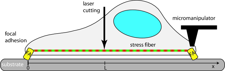
Figure 1: (Color online) Contractile filament bundles are very prominent in cell adhesion. Stress fibers typically connect two focal adhesions and through their contraction, the cell can probe the mechanical properties of the substrate. The viscoelastic properties of stress fibers can be probed by laser cutting or by cyclic loading through a micromanipulator.

Stress fibers are often mechanically anchored to sites of cell-matrix adhesion, are contracted by non-muscle myosin II motors and have a sarcomeric structure similar to muscle Pellegrin and Mellor (2007); Peterson et al. (2004), as shown schematically in Fig. 1. However, their detailed molecular structure is much less ordered than in muscle. In particular, stress fibers in live cells continuously grow out of the focal adhesions Endlich et al. (2007) and tend to tear themselves apart under the self-generated stress Smith et al. (2010). Up to now, the mechanical response of stress fibers has been measured mainly isolated from cells Katoh et al. (1998); Deguchi et al. (2006); Matsui et al. (2009). Recently, pulsed lasers have been employed to disrupt single stress fibers in living cells Kumar et al. (2006); Colombelli et al. (2009); Tanner et al. (2010). By using the intrinsic sarcomeric pattern or an artificial pattern bleached into the fluorescently labeled stress fibers, the contraction dynamics of dissected actin stress fibers has been resolved with high spatial and temporal resolution along their whole length Colombelli et al. (2009). These experiments showed that dissected stress fibers contract non-uniformly and that the total contraction length saturates for long fibers, suggesting that stress fibers in adherent cells are not only attached at their endpoints, but also along their whole length. In the same study, cyclic forces have been applied to stress fibers by an AFM cantilever, mimicking physiological conditions like in heart, vasculature or gut. Fig. 1 shows schematically how laser cutting and micromanipulation are applied to an adherent cell.

Early theory work on stress fibers focused on the dynamics of self-assembly leading to a stable contractile state Kruse and Julicher (2000); Kruse and Julicher (2003). Later more detailed mechanical models have been developed and parametrized by experimental data Besser and Schwarz (2007); Stachowiak and O’Shaughnessy (2008); Luo et al. (2008); Colombelli et al. (2009); Stachowiak and O’Shaughnessy (2009); Russell et al. (2009); Besser and Schwarz (2010). Here we investigate a generic continuum model for the mechanics of contractile filament bundles and show that it can be solved analytically for the boundary conditions corresponding to stress fiber laser nanosurgery and cyclic pulling experiments. Our analytical results can be easily used for analyzing experimental data. For relaxation dynamics after laser cutting, our model predicts unexpected oscillations. We reevaluate data obtained earlier from laser cutting experiments Colombelli et al. (2009) and indeed find evidence for the predicted oscillations.

This paper is organized as follows. In Sec. II we introduce our continuum model, including the central stress fiber equation, Eq. (4). The stress fiber equation is a partial differential equation with mixed spatial and temporal derivatives. In order to solve it analytically, in Sec. III we discretize this equation in space. This results in a system of ordinary differential equations, which can be solved in closed form by an eigenvalue analysis. In Sec. IV, we take the continuum limit of this solution, thus arriving at the general solution of the continuum model. This general solution is given in Eq. (40), with the corresponding spectrum of retardation times given in Eq. (38). In Sec. V and Sec. VI, we specify and discuss the general solution for the boundary conditions appropriate for laser cutting and cyclic loading, respectively. In Sec. VII, we close with a discussion.

II Model definition and solution

We model the effectively one-dimensional stress fiber as a viscoelastic material which is subject to active myosin contraction forces and which interacts viscoelasticly with its surrounding. In the framework of continuum mechanics, the fiber internal viscoelastic stress is given by the viscoelastic constitutive equation Pipkin (1986):

$$\sigma(t)=\int_{-\infty}^{t}G_{int}(t-t^{\prime})\dot{\epsilon}(t^{\prime})dt^{\prime}\ ,$$ (1)

where $\sigma=\sigma_{xx}$ and $\epsilon=\epsilon_{xx}=\partial_{x}u$ denote the relevant components of the stress and strain tensors, respectively. $u(x,t)$ denotes the displacement along the fiber and $G_{int}$ is the internal stress relaxation function. In addition to the viscoelastic stress, the fiber is subject to myosin contractile stress $\sigma_{m}$, which we characterize by a linear stress-strain rate relation ${\sigma_{m}=\sigma_{s}(1+\partial_{x}\dot{u}/\dot{\epsilon}_{0})}$. $\dot{\epsilon}_{0}$ denotes the strain rate of an unloaded fiber and $\sigma_{s}$ is the maximal stress that the molecular motors generate under stalling conditions. In addition to the fiber internal stresses, viscoelastic interactions with the surrounding lead to body forces, $f_{ext}$, that act over a characteristic length $a$ along the fiber and resist the fiber movement:

$$f_{ext}=-\frac{1}{a}\int_{-\infty}^{t}G_{ext}(t-t^{\prime})\dot{u}(t^{\prime})dt^{\prime}\ .$$ (2)

Here, $G_{ext}$ is the external stress relaxation function. In the following we assume that both internal and external stress relaxation functions have the characteristics of a Kelvin-Voigt material:

$$G(t)=K\theta(t)+2\eta\delta(t)$$ (3)

where $K$ and $\eta$ are elastic and viscous parameters, respectively, and $\theta(t)$ and $\delta(t)$ denote the Heaviside step and Dirac delta function, respectively. The chosen Kelvin-Voigt model is the simplest model for a viscoelastic solid that can carry load at constant deformation over a long time. Note that $K_{ext}$ represents the elastic foundation of the stress fibers revealed by the laser cutting experiments Colombelli et al. (2009), while $\eta_{ext}$ represents dissipative interactions between the moving fiber and the cytoplasm.

Our central equation (the stress fiber equation) follows from mechanical equilibrium, $\partial_{x}\left(\sigma+\sigma_{m}\right)+f_{ext}=0$, which results in the following partial differential equation:

$$\partial_{x}^{2}\dot{u}+\partial_{x}^{2}u-\Gamma\dot{u}-\kappa u=0\ .$$ (4)

This equation has been written in non-dimensional form using the typical length scale $a$, the time scale $\tau=\eta_{int}/K_{int}+\sigma_{s}/(\dot{\epsilon}_{0}K_{int})$, the force scale $f_{0}=K_{int}$, the non-dimensional ratio of viscosities $\Gamma=a\eta_{ext}/(\eta_{int}+\sigma_{s}/\dot{\epsilon}_{0})$ and the non-dimensional ratio of stiffnesses $\kappa=aK_{ext}/K_{int}$. Eq. (4) has been derived before via a different route, namely as the continuum limit of a discrete model representing the force balance in each sarcomeric element of a discrete model Besser and Schwarz (2007); Colombelli et al. (2009); Besser and Schwarz (2010). However, the pure continuum viewpoint taken here seems at least equally valid, because stress fibers are more disordered than muscle and because the interactions with the environment represented by $K_{ext}$ and $\eta_{ext}$ are expected to be continuous along the stress fiber. In general, the stress fiber equation (4) can be solved numerically with finite element techniques Besser and Schwarz (2010). In this paper, we show that it also can be solved analytically.

In order to solve the stress fiber equation, we have to impose boundary and initial conditions. We impose the boundary conditions that the fiber is firmly attached at its left end at $x=0$, and is pulled with a certain boundary force $f_{b}(t)$ at its right end at $x=L/a=l$:

$$u(0,t)=0\,\,\,\,\,\,\textrm{and}\,\,\,\,\,\,{\partial_{x}}\dot{u}(l,t)+{\partial_{x}}u(l,t)+f_{s}=f_{b}(t)\ .$$ (5)

The boundary condition for $x=l$ describes the balance of forces at the right end of the fiber where $f(t):=f_{s}-f_{b}(t)$ is the difference between the myosin stall force $f_{s}=\sigma_{s}/f_{0}$ and the externally applied boundary force $f_{b}(t)$. As initial condition, we simply use $u(x,0)=0$, that is vanishing displacement.

Before we derive the general model solution, we briefly discuss the special case $\kappa=\Gamma$. This case can be easily solved and gives first insight into the solution for the displacement field $u(x,t)$. With the definition $h=\dot{u}+u$, the partial differential equation Eq. (4) becomes a homogeneous linear ordinary differential equation:

$$\partial_{x}^{2}h-\kappa h=0$$ (6)

with the boundary conditions $h(0)=0$ and $\partial_{x}h(l)+f(t)=0$. It can be solved by an exponential ansatz and thus leads to a inhomogeneous linear ordinary differential equation $\dot{u}+u=h$ for $u$, with the initial condition $u(x,0)=0$. The final solution reads

$$u(x,t)=-\frac{\sinh(x\sqrt{\kappa})}{\sqrt{\kappa}\cosh(l\sqrt{\kappa})}\int_{0}^{t}f(t^{\prime})e^{-(t-t^{\prime})}dt^{\prime}\ .$$ (7)

Laser cutting experiments correspond to the situation where the externally applied boundary forces vanish, that is $f(t)=f_{s}=\textrm{const}$. Then the integral in Eq. (7) is trivial and thus the special case $\kappa=\Gamma$ leads to a retardation process with a single retardation time $\tau$. The largest, always negative displacement given by $-\frac{f_{s}}{\sqrt{\kappa}}$ occurs at $x=l$, where the fiber was released by the laser cut. The magnitude of the displacement decreases exponentially with increasing distance from this point and the typical length scale of this decay is given by $a/\sqrt{\kappa}$.

III Solution of the discretized model

In order to find a closed analytical solution for the general stress fiber equation, Eq. (4), we discretize our model in space. In order to implement the correct boundary conditions at $x=0$, it is convenient to symmetrize the system. Thus we consider a doubled model with $2N$ units and $2N+1$ nodes as shown in Fig. 2. Like in the continuum model, internal and external stress relaxation are modeled as Kelvin-Voigt-like, that is ($k_{int}$, $\gamma_{int}$) and ($k_{ext}$, $\gamma_{ext}$) are the spring stiffness and the viscosity of the internal and external Kelvin-Voigt elements, respectively. Each internal Kelvin-Voigt body is also subject to the contractile actomyosin force $F_{m_{n}}$ modeled by a linearized force-velocity relationship Howard (2001):

$$F_{m_{n}}=F_{s}(1-\frac{v_{n}}{v_{0}})=F_{s}+\frac{F_{s}}{v_{0}}(\dot{u}_{n}-\dot{u}_{n-1})\ .$$ (8)

$F_{m_{n}}$ is the force exerted by the $n$-th motor moving with velocity $v_{n}$. $v_{0}$ is the zero-load or maximum motor velocity and $F_{s}$ is the stall force of the motor. In the final relation we have used that the contraction velocity of the $n$-th motor, $v_{n}$, can be related to the rate of elongation of the n-th sarcomeric unit as $v_{n}=-(\dot{u}_{n}-\dot{u}_{n-1})$.

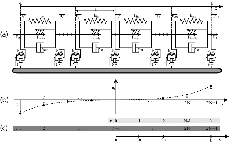
Figure 2: Discretized model. (a) The filament bundle is modeled as a linear chain of Kelvin-Voigt bodies, each characterized by a spring of stiffness $k_{int}$, a dashpot of viscosity $\gamma_{int}$ and a linear extension $a$. Actomyosin contractility is described by a contractile element with contraction force $F_{m}$ added to each Kelvin-Voigt body in parallel. Viscoelastic interactions between fiber elements and their surrounding are described by an additional set of external Kelvin-Voigt bodies with stiffness $k_{ext}$ and viscosity $\gamma_{ext}$. The total fiber length is $L$. $u_{n}$ denotes the displacement of the $n$-th node. (b) Schematic drawing of the solution for the node displacements assuming that both ends are pulled by an external force $F_{b}>F_{s}$. Since both terminating nodes are pulled outward, the solution for the displacements is antisymmetric with respect to the center node at $n=0$, which therefore does not move. Thus we obtain the boundary conditions of interest, clamped at $n=0$ and pulled by $F_{b}$ at $n=N$. (c) The index $n$ starts counting at the center node. The index $j$ starts counting at the node which terminates the fiber at the left.

Our model resembles the Kargin-Slonimsky-Rouse (KSR) model for viscoelastic polymers Kargin and Slonimsky (1948, 1949); Rouse (1953); Vinogradov and Malkin (1980), although it is more complicated due to the presence of active stresses and the elastic coupling to the environment. The main course of our derivation of the solution for the discrete model follows a similar treatment given before for the KSR-model Gotlib and Volkenshtein (1953). The force balance at each node ${j=1,\ldots,2N+1}$ of the fiber as shown in Fig. 2 reads

$$\begin{array}[]{lc}\textrm{For~{}}j=1\textrm{:}&(\dot{u}_{2}-\dot{u}_{1})-\Gamma\dot{u}_{1}+(u_{2}-u_{1})-\kappa u_{1}=-f(t)\\ \textrm{For~{}}j=2,\ldots,2N\textrm{:}&(\dot{u}_{j+1}-2\dot{u}_{j}+\dot{u}_{j-1})-\Gamma\dot{u}_{j}+(u_{j+1}-2u_{j}+u_{j-1})-\kappa u_{j}=0\\ \textrm{For~{}}j=2N+1\textrm{:}&-(\dot{u}_{2N+1}-\dot{u}_{2N})-\Gamma\dot{u}_{2N+1}-(u_{2N+1}-u_{2N})-\kappa u_{2N+1}=f(t)\ .\\ \end{array}$$ (9)

We non-dimensionalized time using the time scale $\tau$, introduced the non-dimensional parameters ($\kappa$, $\Gamma$) and combine all inhomogeneous boundary terms in the function $f(t)$:

$$\tau=~{}\frac{v_{0}\gamma_{int}+F_{s}}{v_{0}k_{int}},\hskip 28.45274pt\kappa=\frac{k_{ext}}{k_{int}}~{},\hskip 28.45274pt\Gamma=\frac{v_{0}\gamma_{ext}}{v_{0}\gamma_{int}+F_{s}}~{},\hskip 28.45274ptf(t)=\frac{F_{s}-F_{b}(t)}{k_{int}}\ .$$ (10)

It is important to note that Eq. (9) is not made non-dimensional in regard to space; this will be done later when the continuum limit is performed.

By taking the difference of subsequent equations in Eq. (9) and by introducing the relative coordinates $y_{j}=u_{j+1}-u_{j}$, we can write

$$\emph{{M}}_{visc}\dot{\vec{y}}+\emph{{M}}_{elas}\vec{y}=\vec{f}(t)$$ (11)

with the $2N\times 2N$ matrix:

$$\emph{{M}}_{visc}=\left(\begin{array}[]{cccl}2+\Gamma&-1&0&\cdots\\ -1&2+\Gamma&-1&\cdots\\ 0&-1&2+\Gamma&\cdots\\ \vdots&\vdots&\vdots&\ddots\\ \end{array}\right)\ .$$ (12)

The matrix $\emph{{M}}_{elas}$ has the same form as $\emph{{M}}_{visc}$, except that $\kappa$ replaces $\Gamma$. In addition we have defined the $2N$-dimensional vectors:

$$\vec{y}(t)=\left(\begin{array}[]{c}y_{1}\\ y_{2}\\ \vdots\\ y_{2N-1}\\ y_{2N}\\ \end{array}\right)\hskip 14.22636pt\text{and}\hskip 14.22636pt\vec{f}(t)=\left(\begin{array}[]{c}-f(t)\\ 0\\ \vdots\\ 0\\ -f(t)\\ \end{array}\right)\ .$$ (13)

We first solve the homogeneous equation. Let $\lambda_{l}$ be an eigenvalue and let $\vec{v}_{l}$ be the associated eigenvector that solves the eigenvalue problem:

$$(\emph{{M}}_{elas}-\lambda_{l}\emph{{M}}_{visc})\vec{v}_{l}=0\ .$$ (14)

Then the general solution of the homogeneous equation is given by:

$$\vec{y}(t)=\sum_{l=1}^{2N}c_{l}\vec{y}_{l}(t)=\sum_{l=1}^{2N}c_{l}\vec{v}_{l}e^{-\lambda_{l}t}$$ (15)

with the eigenvalues and eigenvectors

$$\lambda_{l}=\frac{\kappa+4\sin^{2}(\frac{\pi l}{2(2N+1)})}{\Gamma+4\sin^{2}(\frac{\pi l}{2(2N+1))}}\hskip 8.5359pt\text{and}\hskip 8.5359pt\vec{v}_{l}=\left(\begin{array}[]{c}\sin(\frac{\pi l}{2N+1})\\[11.38092pt] \sin(\frac{\pi 2l}{2N+1})\\[11.38092pt] \sin(\frac{\pi 3l}{2N+1})\\ \vdots\\ \sin(\frac{\pi 2Nl}{2N+1})\\ \end{array}\right)\ .$$ (16)

It is straight forward to check that Eq. (16) is indeed the solution to the eigenvalue problem defined by Eq. (14), see the appendix. There we also prove that the $2N$ eigenvalues are distinct, positive and non-zero, and that the eigenvectors are orthogonal and their length is given by $v_{l}=\sqrt{(2N+1)/2}$. These results validate the form of the homogeneous solution given in Eq. (15).

In order to determine the solution of the inhomogeneous equation, Eq. (11), we use variation of the coefficients:

$$\vec{y}(t)=\sum_{l=1}^{2N}c_{l}(t)\vec{v}_{l}e^{-\lambda_{l}t}\ .$$ (17)

Inserting this ansatz into the inhomogeneous Eq. (11) and using the homogeneous solution yields $2N$ conditions defining the coefficients $c_{l}(t)$:

$$\sum_{l}\dot{c}_{l}(t)\emph{{M}}_{visc}\vec{v}_{l}e^{-\lambda_{l}t}=\vec{f}(t)\ .$$ (18)

Evaluation of the product $\emph{{M}}_{visc}\vec{v}_{l}$, rewriting the $2N$ equations by components, and applying appropriate addition theorems yields

$$\sum_{l=1}^{2N}\dot{c}_{l}(t)\sin(\frac{\pi lj}{2N+1})\left(\Gamma+4\sin^{2}(\frac{\pi l}{2(2N+1)})\right)e^{-\lambda_{l}t}=f_{j}(t)\ .$$ (19)

Here the first sinus term is simply the $j$-th component of the $l$-th eigenvector. We define a new $2N\times 2N$ matrix

$$\textbf{U}_{j,l}=\sqrt{\frac{2}{2N+1}}\sin(\frac{\pi lj}{2N+1})$$ (20)

and a new $2N$-dimensional vector $\vec{b}$

$$b_{l}(t)=\sqrt{\frac{2N+1}{2}}\dot{c}_{l}(t)\left(\Gamma+4\sin^{2}(\frac{\pi l}{2(2N+1)})\right)e^{-\lambda_{l}t}\ .$$ (21)

With these definitions, Eq. (19) can be rewritten as:

$$\emph{{U}}\,\vec{b}(t)=\vec{f}(t)\ .$$ (22)

Because U is built up by the normalized and orthogonal eigenvectors, $\emph{{U}}^{T}\emph{{U}}=I$. Moreover it is symmetric, thus $\emph{{U}}=\emph{{U}}^{T}=\emph{{U}}^{-1}$. Therefore

$$\vec{b}(t)=\emph{{U}}\vec{f}(t)$$ (23)

The only non-zero components of $\vec{f}(t)$ are $f_{1}=f_{2N}=-f(t)$. Therefore the solution for $\vec{b}$ is given by:

$$\begin{array}[]{rcl}\displaystyle b_{l}(t)&\displaystyle=&\displaystyle-f(t)\sqrt{\frac{2}{2N+1}}\left(\sin(\frac{\pi l}{2N+1})+\sin(\frac{\pi 2Nl}{2N+1})\right)\\[14.22636pt] &\displaystyle=&\displaystyle-f(t)\sqrt{\frac{2}{2N+1}}\left(1+(-1)^{l+1}\right)\sin(\frac{\pi l}{2N+1})\ .\end{array}$$ (24)

We conclude that all even-numbered components of $\vec{b}$ vanish. The coefficients $c_{l}(t)$ are obtained by using Eq. (24) and integrating Eq. (21):

$$c_{l}(t)=\left\{\begin{array}[]{cl}0&\,\,\,\,\,\,\,\,\text{if}\,\,\,l\,\,\text{even}\\[17.07182pt] \displaystyle-\frac{4}{2N+1}\,\frac{\sin(\frac{\pi l}{2N+1})}{\Gamma+4\sin^{2}(\frac{\pi l}{2(2N+1)})}\int_{0}^{t}f(t^{\prime})e^{\lambda_{l}t^{\prime}}dt^{\prime}&\,\,\,\,\,\,\,\,\text{if}\,\,\,l\,\,\text{odd}\end{array}\right.$$ (25)

The solution for the relative coordinates follows from Eq. (17):

$$y_{j}(t)=-\frac{4}{2N+1}\sum_{l=1,3,5,\ldots}^{2N}\frac{\sin(\frac{\pi l}{2N+1})\sin(\frac{\pi lj}{2N+1})}{\gamma_{ext}+4\tilde{\gamma}_{int}\sin^{2}(\frac{\pi l}{2(2N+1)})}\int_{0}^{t}f(t^{\prime})e^{-\lambda_{l}(t-t^{\prime})}dt^{\prime}\ .$$ (26)

The actual displacements $u_{j}(t)$ are recovered from the relative coordinates by evaluating the telescoping sum:

$$\begin{array}[]{rcccccccc}u_{2N+1}-u_{1}&=&\underbrace{(u_{2N+1}-u_{2N})}&+&\underbrace{(u_{2N}-u_{2N-1})}&+&\ldots&+&\underbrace{(u_{2}-u_{1})}\\ &=&y_{2N}&+&y_{2N-1}&+&\ldots&+&y_{1}\\[11.38092pt] &=&\displaystyle\sum_{j=1}^{2N}y_{j}\ .\end{array}$$ (27)

Since the solution has to be antisymmetric with respect to the center node at $j=N+1$, compare Fig. 2, it must hold true that $u_{2N+1}=-u_{1}$ and more generally $u_{2N+1-k}=-u_{1+k}$, such that for $k=0,\ldots,N-1$, the displacements are given by:

$$\begin{array}[]{rcl}\displaystyle u_{2N+1-k}&\displaystyle=&\displaystyle\frac{1}{2}\sum_{j=1+k}^{2N-k}y_{j}\\[19.91684pt] &\displaystyle=&\displaystyle\frac{1}{2}\sum_{j=1}^{2N-k}y_{j}-\frac{1}{2}\sum_{j=1}^{k}y_{j}\\[19.91684pt] &\displaystyle=&\displaystyle\frac{1}{2}\sum_{l=1,3,5,\ldots}^{2N}c_{l}(t)e^{-\lambda_{l}t}\left(\sum_{j=1}^{2N-k}\sin(\frac{\pi jl}{2N+1})-\sum_{j=1}^{k}\sin(\frac{\pi jl}{2N+1})\right)\ .\\[19.91684pt] \end{array}$$ (28)

In the last step, we used the solution for the relative coordinates given by Eq. (26) and have subsequently reversed the order of summation in both terms. The two sums in parenthesis can be further simplified by using the identity

$$\sum_{j=0}^{n}\sin(j\alpha)=\frac{1}{2}\left(\cot(\alpha/2)-\frac{\cos(\alpha(n+1/2))}{\sin(\alpha/2)}\right)\ .$$ (29)

Rewriting the result to the index $1\leq n\leq N$, see Fig. 2, we obtain the desired solution of the discrete model:

$$u_{n}(t)=-\frac{2}{2N+1}\sum_{m=1}^{N}\frac{(-1)^{m-1}}{\sin\frac{\pi(2m-1)}{2(2N+1)}}\,\,\frac{\sin\frac{\pi n(2m-1)}{2N+1}\sin\frac{\pi(2m-1)}{2N+1}}{\Gamma+4\sin^{2}\frac{\pi(2m-1)}{2(2N+1)}}\int_{0}^{t}f(t^{\prime})e^{-\frac{t-t^{\prime}}{\tau_{m,N}}}dt^{\prime}$$ (30)

with the retardation times:

$$\tau_{m,N}=\frac{1}{\lambda_{2m-1,N}}=\frac{\Gamma+4\sin^{2}\frac{\pi(2m-1)}{2(2N+1)}}{\kappa+4\sin^{2}\frac{\pi(2m-1)}{2(2N+1)}}\ .$$ (31)

Note that Eq. (30) gives the correct result $u_{0}=0$ for the left boundary. For this reason, we can extend the range of validity of Eq. (30) to $0\leq n\leq N$. We also note that the retardation times depend on the number of units $N$ because the solution describes the movement of a fiber with $N$ units which is attached at its left end $n=0$ and is pulled at its right end $n=N$ with boundary force $f_{b}(t)$. It is straight forward to confirm the validity of the derived discrete solution, Eq. (30) and Eq. (31), by inserting it into the discrete model equation, Eq. (9).

IV Continuum limit of the discretized model

The discrete stress fiber model can be transformed to a continuum equation by considering the limit $N\rightarrow\infty$ while the length $L$ of the fiber is kept constant. In this process, the stress fiber length $L$ is subdivided into incremental smaller pieces of length $a_{N}=L/N$. Thereby it has to be ensured that the effective viscoelastic properties of the whole fiber are conserved. This is accomplished by re-scaling all viscoelastic constants in each iteration step with the appropriate scaling factor $\phi_{N}=\frac{a}{a_{N}}=\frac{Na}{L}$ according to:

$$\begin{array}[]{ccccccc}k_{N,int}&=&\phi_{N}k_{int}&\,\,\,\,\,\,\text{and}&\gamma_{N,int}&=&\phi_{N}\gamma_{int}\\[5.69046pt] k_{N,ext}&=&{\displaystyle\phi_{N}^{-1}k_{ext}}&\,\,\,\,\,\,\text{and}&\gamma_{N,ext}&=&{\displaystyle\phi_{N}^{-1}\gamma_{ext}}\end{array}$$ (32)

To further clarify this procedure consider a single harmonic spring of resting length $a$ and stiffness $k$. This spring is equivalent to two springs of length $a/2$ and stiffness $2k$ that are connected in series. Here, the scaling factor is $\phi_{2}=\frac{a}{a_{2}}=2$. Thus, the stiffness $k_{N,int}$ in Eq. (32) represents the stiffness of a fiber fragment of length $a_{N}$ and increases linearly with the number of partitions $N$, whereas $k_{int}$ is the reference stiffness of a fiber fragment of length $a$. A typical value for the length scale $a$ would be $a=1\,\mu\textrm{m}$, the typical length of sarcomeric units in stress fibers Colombelli et al. (2009). While $k_{N,int}$ increases linearly with the number of partitions, $k_{N,ext}$ decreases according to $1/N$. Similarly it follows that the viscous parameter $\gamma_{N,int}$ and $\gamma_{N,ext}$ scale as $k_{N,int}$ and $k_{N,ext}$, respectively. The non-dimensional parameters and the boundary force scale like:

$$\Gamma_{N}=\phi_{N}^{-2}\Gamma,\hskip 28.45274pt\kappa_{N}=\phi_{N}^{-2}\kappa,\hskip 28.45274ptf_{N}(t)=\phi_{N}^{-1}f(t)\ .$$ (33)

We begin the limiting procedure by introducing the continuous spatial variable $x=na_{N}$, denoting the position of the $n$-th node within the discrete chain with $N$ units. Then Eq. (9) yields (also compare Fig. 2):

$$\begin{array}[]{l}\textrm{For~{}}n=0:\\ u(0)=0\\[8.5359pt] \textrm{For~{}}n=1,\ldots,N\textrm{:}\\ \dot{u}(x+a_{N})-2\dot{u}(x)+\dot{u}(x-a_{N})-\Gamma_{N}\dot{u}(x)+u(x+a_{N})-2u(x)+u(x-a_{N})-\kappa_{N}u=0\\[8.5359pt] \textrm{For~{}}n=N\textrm{:}\\ \dot{u}(L)-\dot{u}(L-a_{N})+\Gamma_{N}\dot{u}(L)+u(L)-u(L-a_{N})+\kappa_{N}u(L)+f_{N}(t)=0\\ \end{array}$$ (34)

Using the scaling relations for the viscoelastic parameters given in Eq. (33) and conducting the limit $N\rightarrow\infty$ yields for $n=1,\ldots,N$:

$$\begin{array}[]{lcl}\displaystyle a^{2}\lim_{N\rightarrow\infty}\left(\frac{\dot{u}(x+a_{N})-2\dot{u}(x)+\dot{u}(x-a_{N})}{{a_{N}}^{2}}\right)-\Gamma\dot{u}(x)&\displaystyle+\ldots&\\[19.91684pt] \displaystyle a^{2}\lim_{N\rightarrow\infty}\left(\frac{u(x+a_{N})-2u(x)+u(x-a_{N})}{{a_{N}}^{2}}\right)-\kappa u(x)&\displaystyle=&\displaystyle 0\end{array}$$ (35)

Since $a_{N}$ is a sequence which converges to zero, the limits define the second derivative of $u$ with respect to $x$. The continuum limit of the upper equation results in a partial differential equation for the displacement $u(x,t)$. The highest order term will contain mixed derivatives in $x$ and $t$, namely, $\partial_{x}^{2}\dot{u}$. Similarly, the limiting process can be performed for the boundary condition at the right end. Note that at this point the spatial variable evaluates to $x=Na_{N}=L$:

$$\begin{array}[]{ll}\displaystyle a\lim_{N\rightarrow\infty}\left(\frac{\dot{u}(L)-\dot{u}(L-a_{N})}{a_{N}}\right)+\Gamma\lim_{N\rightarrow\infty}\frac{a_{N}}{a}\dot{u}(L)+\ldots&\\[19.91684pt] \displaystyle a\lim_{N\rightarrow\infty}\left(\frac{u(L)-u(L-a_{N})}{a_{N}}\right)+\kappa\lim_{N\rightarrow\infty}\frac{a_{N}}{a}u(L)+f(t)=&\displaystyle 0\end{array}$$ (36)

In each line of the equation, the first limit gives the first derivative of $u$ with respect to $x$ evaluated at $x=L$ and the second limit in each line vanishes as $a_{N}$ converges to zero. Consequently, in the continuum representation, the stresses which originate from shearing the environment cannot contribute to the boundary condition. Our continuum model for stress fibers defined by Eq. (4) and Eq. (5) is recovered after non-dimensionalizing $x,L,u,f$ using the typical length scale $a$.

To obtain a closed solution for the continuous model, we apply the continuum limit to the discrete model solution. The limiting procedure is first performed on the retardation times of the discrete model given by Eq. (31):

$$\tau_{m,N}=\frac{\Gamma_{N}+4\sin^{2}\frac{\pi(2m-1)}{2(2N+1)}}{\kappa_{N}+4\sin^{2}\frac{\pi(2m-1)}{2(2N+1)}}=\frac{\Gamma l^{2}+4N^{2}\sin^{2}\frac{\pi(2m-1)}{2(2N+1)}}{\kappa l^{2}+4N^{2}\sin^{2}\frac{\pi(2m-1)}{2(2N+1)}}\ .$$ (37)

Performing the limit $N\rightarrow\infty$ yields the retardation times of the continuum model:

$$\tau_{m}=\frac{4\Gamma l^{2}+\pi^{2}(2m-1)^{2}}{4\kappa l^{2}+\pi^{2}(2m-1)^{2}}\ .$$ (38)

Since $1\leq m\leq\infty$, the upper relation defines infinitely many discrete retardation times, non-dimensionalized by $\tau$. From Eq. (38) we deduce that the retardation times are bounded by the extreme values $\tau_{1}$ and $\tau_{\infty}$ according to:

$$1\leq\tau_{m}\leq\frac{4\Gamma l^{2}+\pi^{2}}{4\kappa l^{2}+\pi^{2}}\,\,\,\,\,\,\text{or}\,\,\,\,\,\,\frac{4\Gamma l^{2}+\pi^{2}}{4\kappa l^{2}+\pi^{2}}\leq\tau_{m}\leq 1\ .$$ (39)

The first relation holds if $\kappa\leq\Gamma$, whereas the second holds if $\kappa\geq\Gamma$. In the special case $\kappa=\Gamma$ the finite range of possible values collapses to the single retardation time $\tau$ which leads to a very simple form of the analytical solution as shown above with Eq. (7).

The limiting procedure applied in Eq. (37) can be carried out similarly on the remaining $N$-dependent terms of the discrete solution given by Eq. (30). This yields our central result, i.e. the solution for the continuous boundary value problem defined by Eq. (4) and Eq. (5):

$$u(x,t)\displaystyle=\displaystyle 8l\sum_{m=1}^{\infty}\frac{(-1)^{m+1}\sin\frac{\pi x(2m-1)}{2l}}{4\Gamma l^{2}+\pi^{2}(2m-1)^{2}}\int_{0}^{t}(f_{b}(t^{\prime})-f_{s})e^{-\frac{t-t^{\prime}}{\tau_{m}}}dt^{\prime}$$ (40)

Eq. (40) in combination with Eq. (38) is the general solution of our continuum model. We successfully checked the validity of our analytical solution by comparision with a numerical solution of Eq. (4). One big advantage of the analytical solution is that it can be easily used to evaluate experimental data. In the following, we will discuss its consequences for the two special cases of laser cutting and cyclic loading.

V Laser cutting

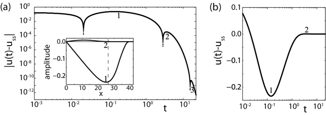
Figure 3: First oscillation. (a) If $\Gamma<\kappa$, the displacements of inner fiber segments exhibit damped oscillations around their final steady state $u_{ss}(x)$. Here we show a log-log-plot of the time course of the absolute difference $|u(x,t)-u_{ss}(x)|$ calculated from Eq. (41) for the position $x=26.4$, which is close to the position with maximal amplitude and corresponds to the band $n=7$ in Fig. 6. The inset gives the amplitudes of the first and second oscillation along the fiber, with maxima $236\,\textrm{nm}$ and 9 nm, respectively. The position $x=26.4$ used here is highlighted as dashed line. (b) The difference $u(x,t)-u_{ss}$ at the position $x=26.4$ is shown on a linear scale. Numbering of the extremal values are included for comparison with (a). Parameters for (a) and (b) are as in Fig. 6: $(\kappa,f_{s},\Gamma)=(0.028,0.39,0)$ and $l=42.2$, ${a=1\,\mu\textrm{m}}$.

If a fiber is cut by a train of laser pulses, then there are no external forces acting anymore on the free fiber end and $f_{b}(t)$ vanishes. Then Eq. (40) can be written as:

$$u(x,t)=\sum_{m=1}^{\infty}S_{m}(x)\left(1-e^{-\frac{t}{\tau_{m}}}\right)\ .$$ (41)

The solution for the displacement can be understood as a retardation process with infinitely many discrete retardation times $\tau_{m}$ given by Eq. (38) and associated, spatially dependent amplitudes $S_{m}(x)$. The amplitudes are given by:

$$S_{m}(x)=8f_{s}l\frac{(-1)^{m}\sin\frac{\pi x(2m-1)}{2l}}{4\kappa l^{2}+\pi^{2}(2m-1)^{2}}\ .$$ (42)

The solution for the displacement at $x=l$, the position of the cut, is particularly simple. At this special position, the amplitudes have a linear relation to the corresponding retardation times:

$$S_{m}(l)=-\frac{2f_{s}}{l}\frac{1-\tau_{m}}{\kappa-\Gamma}\ .$$ (43)

Since the range of possible retardation times is bounded according to Eq. (39), it follows that the spectrum at $x=l$ has only negative amplitudes and the resulting solution for the displacement at $x=l$ is always a monotonically decreasing function. However, this is not true for arbitrary $x$. Inspection of Eq. (42) yields that negative as well as positive amplitudes appear simultaneously. Since $x=l$ evaluates the numerator in Eq. (42) at its maximum, the resulting spectrum constitutes a lower bound for the negative amplitudes of the spectra with $x\neq l$. Similarly, the absolute value of Eq. (43) gives an upper bound for all positive amplitudes. Thus, the retardation spectra with $x\neq l$ oscillate around zero within an envelope for the amplitudes that decays linearly toward zero. This can lead to damped oscillations in the displacement of inner fiber bands about their stationary value. An representative time course is shown in Fig. 3. The emergence of these oscillations is particularly interesting since the stress fiber is modeled in the overdamped limit, that is, inertia terms are neglected. We find that these damped oscillations in this inertia-free system occur only for $\Gamma/\kappa<1$, but then for all positions $x\neq l$. The amplitude of these oscillations reach their maximum at distinct positions along the fiber, as shown by the inset to Fig. 3. The location of the maxima moves further away from the cut (toward smaller $x$-values) with increasing order of the oscillation. Fig. 3 shows the time course of the displacement at $x=26.4$ which is close to the position where the first oscillation reaches its maximum. Using the same parameters as in Fig. 3, we show in Fig. 4 the time course of the displacement at $x=11.0$ where the second oscillation reaches its maximum. Since the oscillations are strongly damped, the maximum amplitude of the oscillations also decreases with the order. While the maximal amplitude of the first oscillation can reach hundreds of nanometers ($236\,\textrm{nm}$ at $x=24.9$, see inset to Fig. 3), the maximal amplitude of the second oscillation is already much smaller and only of the order of tens of nanometers ($9\,\textrm{nm}$ at $x=11.0$, see Fig. 4). Thus, in order to detect the oscillations in experiments, it is essential to measure close to where the oscillations reach their respective maximum amplitude. We demonstrate this by showing predicted time courses of the difference $u(x,t)-u_{ss}$ at the two positions in Fig. 3 (b) and Fig. 4 (b), respectively. While the first oscillation is most prominent in Fig. 3 (b), the second oscillations is not detectable at this position. In contrast, the amplitude of the first oscillation in Fig. 4 (b) is reduced compared to Fig. 3 (b) but the amplitude of the second oscillation is much larger and becomes detectable.

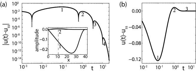
Figure 4: Second oscillation. (a) Time course of the absolute difference $|u(x,t)-u_{ss}|$ on a log-log-scale at the position $x=11.0$, where the amplitude of the second oscillation attains its maximum. The inset again shows the maximum amplitude of the first and second oscillation along the fiber, but now the position $x=11.0$ is highlighted as dashed line. (b) The difference $u(x,t)-u_{ss}$ at the position $x=11.0$ is shown on a linear scale. Numbering of the extremal values are included for comparison with (a). Parameters used for (a) and (b) are the same as in Fig. 3 and Fig. 6.

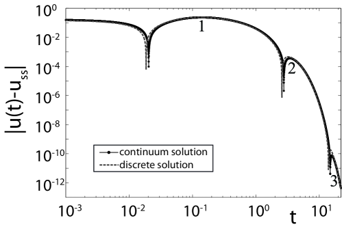
Figure 5: Comparision of $|u(x,t)-u_{ss}(x)|$ for the continuum model (solid) and for the discrete model (dashed). The continuum solution is calculated for a fiber of length $l=42$ at position $x=26$. The discrete solution is calculated for a fiber with $N=42$ subunits at node $n=26$. Both solutions were calculated for the same parameters $(\kappa,\Gamma,f_{s})=(0.028,0,0.39)$ as extracted from experimental data. The two solutions agree well with each other and both models predict oscillations.

To show that the oscillations are not an artifact introduced by the continuum limit, we have compared solutions of corresponding continuous and discrete models. Results are shown in Fig. 5 where we have used the same parameters as for Fig. 3 and Fig. 4. To facilitate comparison between continuum and discrete model, solutions are calculated for integer fiber lengths and integer positions. We find that continuum and discrete solution agree very well and, most importantly, both predict oscillations when $\Gamma<\kappa$.

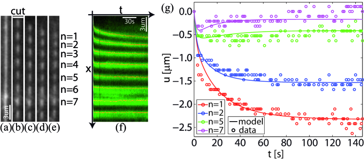
Figure 6: (Color online) Experimental results. (a) GFP-actin stress fiber prior to patterning by photo bleaching, scale bar: $3~{}\mu\textrm{m}$. (b) Fiber bleached with stripe pattern. (c-e) Stress fiber $1\,\textrm{s}$, $30\,\textrm{s}$ and $140\,\textrm{s}$ after laser cutting. (f) Time-space kymograph reconstructed from fluorescence intensity profiles along the stress fiber. Band positions are extracted by edge-detection (solid lines), scale bars: $30~{}\textrm{s}$ and $3~{}\mu\textrm{m}$. (g) Model fit to the displacement data of shown bands (n increasing from bottom to top) with initial positions $x_{n=1,2,5,7}=(42.2,39.7,31.8,26.4)\mu\textrm{m}$ yields $(\kappa,f_{s},\tau,\Gamma)=(0.028,0.39,34\,\textrm{s},0.0)$ with $a=1.0\,\mu\textrm{m}$. Note that $\Gamma/\kappa\ll 1$ and that the experimental data provide evidence for the predicted oscillations, because the curves for n=5 and 7 show dips at 8s and 5s after cutting, respectively.

Because of the analytical solution Eq. (41), we can easily apply our model to evaluate experimental data for stress fiber contraction dynamics induced by laser nano-surgery Colombelli et al. (2009). Briefly, Ptk-2 cells were tranfected with GFP-actin and a stripe pattern was bleached into their stress fibers. 10 s later the stress fibers were cut with a laser and their retraction was recorded over several minutes. Kymographs were constructed and for each band, the retraction trace was extracted by edge detection. Least-square fitting of the theoretical predictions to four selected bands simultaneously was used to estimate the four model parameters ($\kappa,f_{s},\tau,\Gamma$). An representative example for the outcome of this procedure is shown in Fig. 6 (more examples and the details of our experiments are provided in the supplementary material). We find that $\Gamma=(0.52\pm 0.23)\cdot 10^{-3}\ll 1$ and $\Gamma/\kappa=0.013\pm 0.021\ll 1$ (mean $\pm$ std, $N=6$). This means that in our experiments the second relation of Eq. (39) applies and that the oscillations demonstrated by Fig. 3 are predicted for this experimental system. For the positions corresponding to bands $n=5$ and $n=7$ our model predicts minima at $8\,\textrm{s}$ and $5\,\textrm{s}$, respectively. Indeed these minima appear as dips in the experimental data shown in Fig. 6(g).

VI Cyclic loading

The response of stress fibers to cyclic loading is characterized by the complex modulus which we derive from the general solution Eq. (40) by assuming a cyclic boundary force $f_{b}(t)=f_{s}+f_{0}e^{i\omega t}$, with a constant offset compensating the stall force of the molecular motors. Evaluation of the resulting integral in Eq. (40) yields:

$$u(x,t)=8lf_{0}\sum_{m=1}^{\infty}\frac{(-1)^{m+1}\sin\frac{\pi x(2m-1)}{2l}}{4\kappa l^{2}+\pi^{2}(2m-1)^{2}}\,\frac{1}{i\omega\tau_{m}+1}\left(e^{i\omega t}-e^{-\frac{t}{\tau_{m}}}\right)\ .$$ (44)

Inspection of the time-dependent terms yields that the solution for the displacements approaches a harmonic oscillation. The deviations decay exponentially in time, according to $e^{-t/\tau_{m}}$. As a consequence, in the limit for large times, the fiber displacements also oscillate with the same frequency $\omega$ as the force input, but the stationary phase shift between displacements $u(x,t)$ and $f_{b}(t)$ might vary spatially along the fiber. In the following, we are only interested in the response of the fiber as a whole, i.e. we focus on the displacement at $x=l$. With the above arguments, we find in the limit for large times:

$$\begin{array}[]{rcc}\displaystyle u(l,t)=&\displaystyle\underbrace{\sum_{m=1}^{\infty}\frac{8l}{4\kappa l^{2}+\pi^{2}(2m-1)^{2}}\,\frac{1}{i\omega\tau_{m}+1}}\cdot&\displaystyle f_{0}e^{i\omega t}\ .\\[14.22636pt] &\displaystyle=1/\mathcal{G}^{*}(\omega)&\\ \end{array}$$ (45)

The complex modulus, non-dimensionalized by $K_{int}$, can be deduced from Eq. (45) by noting that the cyclic force input $f_{0}e^{i\omega t}$ and the creep response of the fiber $u(l,t)$ are connected by the inverse of the complex modulus Pipkin (1986). The expression for the complex modulus can be separated into its real and imaginary part, the storage and the loss modulus, respectively:

$$\begin{array}[]{rcc}\displaystyle\mathcal{G}^{*}(\omega)=&\displaystyle\underbrace{\frac{p(\omega)}{p^{2}(\omega)+q^{2}(\omega)}}+&\displaystyle i\underbrace{\frac{q(\omega)}{p^{2}(\omega)+q^{2}(\omega)}}\\[14.22636pt] &\displaystyle=\mathcal{G}^{\prime}(\omega)&\displaystyle=\mathcal{G}^{\prime\prime}(\omega)\\ \end{array}$$ (46)

with

$$\begin{array}[]{rl}p(\omega)=&\displaystyle 8l\sum_{m=1}^{\infty}\frac{1}{4\kappa l^{2}+\pi^{2}(2m-1)^{2}}\,\frac{1}{\omega^{2}\tau^{2}_{m}+1}\ ,\\[19.91684pt] q(\omega)=&\displaystyle 8l\sum_{m=1}^{\infty}\frac{1}{4\kappa l^{2}+\pi^{2}(2m-1)^{2}}\,\frac{\omega\tau_{m}}{\omega^{2}\tau^{2}_{m}+1}\ .\\ \end{array}$$ (47)

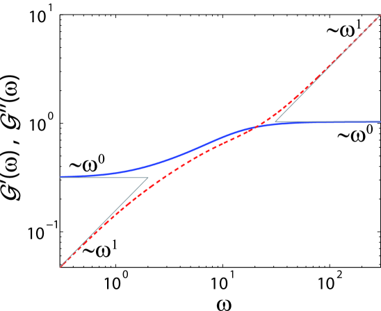
Figure 7: (Color online) Log-log plot of storage modulus (solid) and loss modulus (dashed). Scaling at low and high frequencies is shown for both storage and loss modulus. Used parameters are $(\kappa,\Gamma)=(0.1,0)$ and $l=30$.

An alternative, more concise expression for the complex modulus can be derived by solving the Laplace-transformed model equation for the situation of a sudden force application, $f_{b}(t)=f_{s}+f_{0}\theta(t)$, where $\theta(t)$ is the unit step function. Solution of this Laplace-transformed boundary value problem for $\bar{u}(l,s)=\int_{0}^{\infty}u(l,t)e^{-st}$, with $s=\gamma+i\omega$, directly yields the Laplace-transformed creep compliance, $\bar{J}(s)=\bar{u}(l,s)/f_{0}$. It is connected to the complex modulus by:

$$\mathcal{G}^{*}(\omega)=\lim_{\gamma\rightarrow 0}\frac{1}{s\bar{J}(s)}=\frac{\sqrt{1+i\omega}\sqrt{i\Gamma\omega+\kappa}}{\tanh\left(l\frac{\sqrt{i\Gamma\omega+\kappa}}{\sqrt{1+i\omega}}\right)}\ .$$ (48)

Eq. (46) or Eq. (48) are equivalent expressions for the complex modulus of the stress fiber model. To further study its frequency dependence we use Eq. (48). In the special case $\Gamma/\kappa=1$, it simplifies to $\mathcal{G}^{*}(\omega)=(1+i\omega)\sqrt{\kappa}/\tanh(l\sqrt{\kappa})$. The storage modulus becomes a constant, and the loss modulus is linearly dependent on the frequency. These are the characteristics of a Kelvin-Voigt body. The more the ratio $\Gamma/\kappa$ differs from unity, the larger are the deviations from these simple characteristics. To study the general case $\Gamma/\kappa\neq 1$, consider the limits $\omega\rightarrow 0$ and $\omega\rightarrow\infty$. In both limits, the stress fiber model again exhibits the characteristics of a Kelvin-Voigt body. The explicit values for the limit $\omega\rightarrow 0$ are:

$$\begin{array}[]{rl}\displaystyle\mathcal{G}_{0}^{\prime}=&\displaystyle\sqrt{\kappa}\coth(l\sqrt{\kappa})\\[14.22636pt] \displaystyle\mathcal{G}_{0}^{\prime\prime}(\omega)=&\displaystyle\frac{1}{4\kappa}\operatorname{csch}^{2}(l\sqrt{\kappa})\left(2l\kappa(\kappa-\Gamma)+\sqrt{\kappa}(\kappa+\Gamma)\sinh(2l\sqrt{\kappa})\right)\omega.\\ \end{array}$$ (49)

Similarly, in the limit $\omega\rightarrow\infty$, we find:

$$\begin{array}[]{rl}\displaystyle\mathcal{G}_{\infty}^{\prime}=&\displaystyle\frac{1}{4\Gamma}\operatorname{csch}^{2}(l\sqrt{\Gamma})\left(2l\Gamma(\Gamma-\kappa)+\sqrt{\Gamma}(\Gamma+\kappa)\sinh(2l\sqrt{\Gamma})\right)\\[14.22636pt] \displaystyle\mathcal{G}_{\infty}^{\prime\prime}(\omega)=&\displaystyle\sqrt{\Gamma}\coth(l\sqrt{\Gamma})\omega.\\ \end{array}$$ (50)

It holds that $\mathcal{G}_{\infty}^{\prime}/\mathcal{G}_{0}^{\prime}\geq 1$, with equality for $\Gamma=\kappa$. A similar relation holds for the slope of the loss modulus at high and low frequencies. Fig. 7 shows the predicted frequency dependences of $\mathcal{G}^{\prime}$ and $\mathcal{G}^{\prime\prime}$.

VII Discussion

Here we have presented a complete analytical solution of a generic continuum model for the viscoelastic properties of actively contracting filament bundles. Our model contains the most important basic features which are known to be involved in the function of stress fibers, namely internal viscoelasticity, active contractility by molecular motors, and viscous and elastic coupling to the environment. The resulting stress fiber equation, Eq. (4), can be solved with numerical methods for partial differential equations. In this paper, we have shown that a general solution can be derived by first discretizing the equation in space. In order to implement the correct boundary conditions, the system is symmetrized by doubling its size. The resulting system of ordinary differential equations leads to an eigenvalue problem which can be solved exactly, leading to Eq. (30). A continuum limit needs to take care of the appropriate rescaling of the viscoelastic parameters and finally leads to the general solution Eq. (40) for the stress fiber equation. The validity of our analytical solution has been successfully checked by comparing it with both the discrete and numerical solutions.

Due to their analytical nature, our results can be easily used to evaluate experimental data. Here we have demonstrated this for the case of laser cutting of stress fibers. In an earlier experimental study Colombelli et al. (2009), we focused on the movement of the first three bands ($n=1,2,3$) of the stress fiber. These bands are within less than $10~{}\mu\textrm{m}$ from the fiber tip and thus we did not report the oscillatory feature of bands farther away from the cut. After prediction of these oscillations by our analytical results, we evaluated the experimental data in this respect and indeed found evidence for their occurance (Fig. 6 and supplementary material). This was possible with conventional light microscopy because the amplitude of the first oscillation can reach hundreds of nanometers. The amplitude of the second oscillation, however, is predicted to be typically on the order of tens of nanometers, which is below our resolution limit. In the future, super-resolution microscopy or single particle tracking might allow a nanometer-precise validation of our theoretical predictions.

The extracted parameter values suggest that the frictional coupling between stress fiber and cytoplasm, quantified by $\Gamma$, is not relevant in our experiments, and that the retraction dynamics is dominated by the elastic foundation quantified by $\kappa$ Colombelli et al. (2009). However, the elastic coupling to the environment might depend on cell type and substrate coating. In fact our findings differ from the results of an earlier study, which neglected elastic, but predicted high frictional coupling Stachowiak and O’Shaughnessy (2009). In our model, high frictional coupling corresponds to $\Gamma/\kappa>1$ and thus no oscillations are expected in this case. It would be interesting to cut stress fibers in cells grown on micro-patterned surfaces that prevent substrate attachment along the fiber. We then would expect not only the transition from elastic to viscous coupling, but also the disappearance of the oscillations.

As a second application of our theoretical results, we suggest to measure the viscoelastic response function $G(\omega)$ of single stress fibers. This could be done with AFM or similar setups either on live cells Colombelli et al. (2009) or on single stress fibers extracted from cells Katoh et al. (1998); Deguchi et al. (2006); Matsui et al. (2009). In this case, our model could provide a valuable basis for evaluating changes in the viscoelastic properties of stress fibers induced by changes in motor regulation, e.g. by calcium concentration or pharmacological compounds.

In summary, our analytical results of a generic model open up the perspective of quantitatively evaluating the physical properties for any kind of contractile filament bundle. In order to apply this approach to more complicated cellular or biomimetic systems, it would be interesting to go beyond the one-dimensional geometry of bundles and to also consider higher dimensional arrangements of contractile elements Gittes et al. (1997); Gardel et al. (2004); Mizuno et al. (2007); Koenderink et al. (2009); Fabry et al. (2001); Fernández et al. (2006), which could be modeled for example by appropriately modified two- and three-dimensional networks Coughlin and Stamenovic (2003); Paul et al. (2008); Bischofs et al. (2008).

VIII Acknowledgments

EHKS and USS are members of the Heidelberg cluster of excellence CellNetworks. USS was supported by the Karlsruhe cluster of excellence Center for Functional Nanostructures (CFN) and by the MechanoSys-grant from the Federal Ministry of Education and Research (BMBF) of Germany. AB was supported by the NIH Grant R01 GM071868 and by the German Research Foundation (DFG) through fellowship BE4547/1-1.

IX Appendix: Proofs for eigenvalues and eigenvectors

In the main text we have used the eigenvalues and eigenvectors given by Eq. (16) without proving that this system indeed solves the eigenvalue problem defined by Eq. (14). Here, we verify the solution to the eigenvalue problem and prove the following properties of the eigenvalues and eigenvectors:

1. The eigenvalues are distinct, positive and non-zero.

2. The eigenvectors are orthogonal and their length is given by $v_{l}=\sqrt{(2N+1)/2}$

In order to verify the given eigenvalues and eigenvectors, we first rewrite the matrix $\emph{{M}}_{elas}-\lambda_{l}\emph{{M}}_{visc}$ as:

$$\emph{{M}}_{elas}-\lambda_{l}\emph{{M}}_{visc}=\left(\begin{array}[]{cccl}2B-A&-B&0&\cdots\\ -B&2B-A&-B&\cdots\\ 0&-B&2B-A&\cdots\\ \vdots&\vdots&\vdots&\ddots\\ \end{array}\right)$$ (51)

Where $B=1-\lambda_{l}$ and $A=-\kappa+\lambda_{l}\Gamma$. By using Eq. (16) one can express $A$ in terms of $B$:

$$A=4B\sin^{2}\frac{\pi l}{2(2N+1)}$$ (52)

Substitution of this relation into Eq. (51) and the application of the addition theorem $\cos 2\alpha=1-2\sin^{2}\alpha$ yields:

$$\begin{array}[]{lcl}\emph{{M}}_{elas}-\lambda_{l}\emph{{M}}_{visc}=&B\left(\begin{array}[]{cccl}2\cos\left(\frac{\pi l}{2N+1}\right)&-1&0&\cdots\\ -1&2\cos\left(\frac{\pi l}{2N+1}\right)&-1&\cdots\\ 0&-1&2\cos\left(\frac{\pi l}{2N+1}\right)&\cdots\\ \vdots&\vdots&\vdots&\ddots\\ \end{array}\right)&=:B\emph{{M}}_{l}\end{array}$$ (53)

To prove Eq. (14) it has to be shown that the product $\emph{{M}}_{l}\vec{v}_{l}$ vanishes for all $l=1,\ldots,2N$. The $m$-th component of the vector which results from this product is given below. It simplifies to zero after application of the addition theorem $2\cos\alpha\,\sin\beta=\sin(\alpha+\beta)+\sin(\beta-\alpha)$:

$$-\sin\left(\frac{\pi(m-1)l}{2N+1}\right)+2\cos\left(\frac{\pi l}{2N+1}\right)\sin\left(\frac{\pi ml}{2N+1}\right)-\sin\left(\frac{\pi(m+1)l}{2N+1}\right)=0$$ (54)

Thus we have shown that the system of eigenvalues and eigenvector Eq. (16) indeed solves the eigenvalue problem Eq. (14).

Next we show that the eigenvalues are distinct, positive and non-zero. The fact that the eigenvalues are positive and non-zero follows directly by inspection of Eq. (16) and by noting that all viscoelastic constants are positive. It remains to be shown that there are no multiple eigenvalues. This can be seen after reformulating the expression for the eigenvalues as:

$$\lambda_{l}=1+\frac{\kappa-\Gamma}{\Gamma+4\sin^{2}\frac{\pi l}{2(2N+1)}}$$ (55)

Since $1\leq l\leq 2N$, it holds for the argument of the $\sin$-function that $0<\frac{\pi l}{2(2N+1)}<\frac{\pi}{2}$. In this interval, the $\sin$-function increases monotonically and is single-valued. For this reason, the eigenvalues, $\lambda_{l}$, are also single-valued. The eigenvalues increase monotonically with $l$ if $\kappa<\Gamma$ and decrease monotonically for increasing $l$ if the opposite inequality holds.

Next we show that the eigenvectors are orthogonal and their length is given by $v_{l}=\sqrt{(2N+1)/2}$. Consider the matrix of normalized eigenvectors, U, defined in the main text Eq. (20). By means of this matrix, the statement to be shown can be recapitulated as $\emph{{U}}^{T}\emph{{U}}=I\Leftrightarrow(\emph{{U}}\emph{{U}})_{k,m}=\delta_{k,m}$. The second relation follows since U is obviously symmetric. In the following we will evaluate the square of the matrix U by components:

$$\begin{array}[]{rl}\displaystyle(\emph{{U}}\emph{{U}})_{k,m}&\displaystyle=\sum_{j=1}^{2N}\emph{{U}}_{k,j}\emph{{U}}_{j,m}\\[14.22636pt] &\displaystyle=\frac{2}{2N+1}\sum_{j=1}^{2N}\sin\frac{\pi kj}{2N+1}\sin\frac{\pi jm}{2N+1}\\[14.22636pt] &\displaystyle=\displaystyle\frac{1}{2N+1}\sum_{j=1}^{2N}\left(\cos\frac{\pi j(k-m)}{2N+1}-\cos\frac{\pi j(k+m)}{2N+1}\right)\\[14.22636pt] \end{array}$$ (56)

The finite sums over the $\cos$-functions can be evaluated by expressing it in terms of exponential functions. The used identity is:

$$\begin{array}[]{rcl}\displaystyle\sum_{j=0}^{n}\cos(j\alpha)&\displaystyle=&\displaystyle\frac{1}{2}\left(1+\frac{\sin(\alpha(n+1/2))}{\sin(\alpha/2)}\right)\\[14.22636pt] \end{array}$$ (57)

Application of Eq. (57) in order to simplify Eq. (56) finally yields:

$$\begin{array}[]{rl}\displaystyle(\emph{{U}}\emph{{U}})_{k,m}&\displaystyle=\frac{1}{2(2N+1)}\left(\sin\left((k-m)\pi\right)\cot\frac{(k-m)\pi}{2(2N+1)}\right.\\[14.22636pt] &\displaystyle\left.\hskip 8.5359pt-\sin((k+m)\pi)\cot\frac{(k+m)\pi}{2(2N+1)}\right.\\[14.22636pt] &\displaystyle\left.\hskip 8.5359pt+\cos((k+m)\pi)-\cos((k-m)\pi)\right)\end{array}$$ (58)

There are two cases, namely $k=m$ and $k\neq m$, that have to be considered.

First assume that $k=m$. In this case, the last two terms in Eq. (58) just cancel out each other. The $\sin$-function in the second term evaluates to zero while the cotangent gives a finite value: since $0<\frac{(k+m)\pi}{2(2N+1)}<\pi$, the singularities are just spared. Thus, also this term vanishes. It is only the first term that gives a contribution. Using l’Hôpital’s rule, it evaluates to:

$$\begin{array}[]{rl}\displaystyle(\emph{{U}}\emph{{U}})_{k,k}&\displaystyle=\frac{1}{2(2N+1)}\lim_{m\rightarrow k}\frac{\sin\left((k-m)\pi\right)}{\sin\frac{(k-m)\pi}{2(2N+1)}}\\[14.22636pt] &\displaystyle=\lim_{m\rightarrow k}\frac{\cos\left((k-m)\pi\right)}{\cos\frac{(k-m)\pi}{2(2N+1)}}=1\end{array}$$ (59)

This result ensures that all diagonal components of $\emph{{U}}^{2}$ are unity.

Next assume that $k\neq m$. In this case the first as well as the second term in Eq. (58) vanish since the $\sin$-function evaluates to zero while the co-tangent yields finite values. The last two terms further simplify to:

$$\begin{array}[]{rcl}\displaystyle(\emph{{U}}\emph{{U}})_{k,m\neq k}&\displaystyle=&\displaystyle\frac{1}{2(2N+1)}\left((-1)^{k+m}-(-1)^{k-m}\right)\\[14.22636pt] &\displaystyle=&\displaystyle\frac{1}{2(2N+1)}(-1)^{k-m}\left((-1)^{2m}-1)\right)=0\end{array}$$ (60)

This result ensures that all off-diagonal components of $\emph{{U}}^{2}$ vanish. The combination of Eq. (59) and Eq. (60) yields $(\emph{{U}}\emph{{U}})_{k,m}=\delta_{k,m}$ which was to be demonstrated. Thus we have shown that all eigenvectors are of length $v_{l}=\sqrt{(2N+1)/2}$ and form a complete orthogonal basis.

References

- Gittes et al. (1997) F. Gittes, B. Schnurr, P. D. Olmsted, F. C. MacKintosh, and C. F. Schmidt, Phys. Rev. Lett. 79, 3286 (1997).
- Gardel et al. (2004) M. L. Gardel, J. H. Shin, F. C. MacKintosh, L. Mahadevan, P. Matsudaira, and D. A. Weitz, Science 304, 1301 (2004).
- Mizuno et al. (2007) D. Mizuno, C. Tardin, C. F. Schmidt, and F. C. MacKintosh, Science 315, 370 (2007).
- Koenderink et al. (2009) G. H. Koenderink, Z. Dogic, F. Nakamura, P. M. Bendix, F. C. MacKintosh, J. H. Hartwig, T. P. Stossel, and D. A. Weitz, Proc. Nat. Acad. Sci. 106, 15192 (2009).
- Fabry et al. (2001) B. Fabry, G. N. Maksym, J. P. Butler, M. Glogauer, D. Navajas, and J. J. Fredberg, Phys. Rev. Lett. 87, 148102 (2001).
- Fernández et al. (2006) P. Fernández, P. A. Pullarkat, and A. Ott, Biophys. J. 90, 3796 (2006).
- Discher et al. (2005) D. E. Discher, P. Janmey, and Y.-L. Wang, Science 310, 1139 (2005).
- Vogel and Sheetz (2006) V. Vogel and M. Sheetz, Nat. Rev. Mol. Cell Biol. 7, 265 (2006).
- Geiger et al. (2009) B. Geiger, J. P. Spatz, and A. D. Bershadsky, Nat. Rev. Mol. Cell Biol. 10, 21 (2009).
- Pellegrin and Mellor (2007) S. Pellegrin and H. Mellor, J. Cell Sci. 120, 3491 (2007).
- Peterson et al. (2004) L. J. Peterson, Z. Rajfur, A. S. Maddox, C. D. Freel, Y. Chen, M. Edlund, C. Otey, and K. Burridge, Mol. Biol. Cell 15, 3497 (2004).
- Endlich et al. (2007) N. Endlich, C. Otey, W. Kriz, and K. Endlich, Cell Mot. Cytoskel. 64, 966 (2007).
- Smith et al. (2010) M. Smith, E. Blankman, M. Gardel, L. Luettjohann, C. Waterman, and M. Beckerle, Dev. Cell 19, 365 (2010).
- Katoh et al. (1998) K. Katoh, Y. Kano, M. Masuda, H. Onishi, and K. Fujiwara, Mol. Biol. Cell 9, 1919 (1998).
- Deguchi et al. (2006) S. Deguchi, T. Ohashi, and M. Sato, J. Biomech. 39, 2603 (2006).
- Matsui et al. (2009) T. Matsui, S. Deguchi, N. Sakamoto, T. Ohashi, and M. Sato, Biorheology 46, 401 (2009).
- Kumar et al. (2006) S. Kumar, I. Maxwell, A. Heisterkamp, T. Polte, T. Lele, M. Salanga, E. Mazur, and D. Ingber, Biophys. J. 90, 3762 (2006).
- Colombelli et al. (2009) J. Colombelli, A. Besser, H. Kress, E. Reynaud, P. Girard, E. Caussinus, U. Haselmann, J. Small, U. S. Schwarz, and E. Stelzer, J. Cell Sci. 122, 1665 (2009).
- Tanner et al. (2010) K. Tanner, A. Boudreau, M. Bissell, and S. Kumar, Biophys. J. 99, 2775 (2010).
- Kruse and Julicher (2000) K. Kruse and F. Julicher, Phys. Rev. Lett. 85, 1778 (2000).
- Kruse and Julicher (2003) K. Kruse and F. Julicher, Phys. Rev. E 67 (2003).
- Besser and Schwarz (2007) A. Besser and U. S. Schwarz, New J. Phys. 9, 425 (2007).
- Stachowiak and O’Shaughnessy (2008) M. R. Stachowiak and B. O’Shaughnessy, New J. Phys. 10, 025002 (2008).
- Luo et al. (2008) Y. Luo, X. Xu, T. Lele, S. Kumar, and D. E. Ingber, J. Biomech. 41, 2379 (2008).
- Stachowiak and O’Shaughnessy (2009) M. R. Stachowiak and B. O’Shaughnessy, Biophys. J. 97, 462 (2009).
- Russell et al. (2009) R. Russell, S. Xia, R. Dickinson, and T. Lele, Biophys. J. 97, 1578 (2009).
- Besser and Schwarz (2010) A. Besser and U. S. Schwarz, Biophys. J. 99, L10 (2010).
- Pipkin (1986) A. Pipkin, Lectures on Viscoelasticity Theory, Applied Mathematical Sciences (Springer, New York, 1986).
- Howard (2001) J. Howard, Mechanics of motor proteins and the cytoskeleton (Sunderland, Sinauer Associates, 2001).
- Kargin and Slonimsky (1948) V. A. Kargin and G. L. Slonimsky, Doklady Akademii Nauk SSSR 62, 239 (1948).
- Kargin and Slonimsky (1949) V. A. Kargin and G. L. Slonimsky, Zurnal Fiziceskoj Chimii 23, 563 (1949).
- Rouse (1953) P. E. Rouse, The Journal of Chemical Physics 21, 1272 (1953).
- Vinogradov and Malkin (1980) G. V. Vinogradov and A. Y. Malkin, Rheology of polymers: Viscoelasticity and flow of polymers (Springer-Verlag, Berlin, 1980).
- Gotlib and Volkenshtein (1953) Y. Y. Gotlib and M. V. Volkenshtein, Zurnal Techniceskoj Fiziki 23, 1936 (1953).
- Coughlin and Stamenovic (2003) M. F. Coughlin and D. Stamenovic, Biophys J. 84, 1328 (2003).
- Paul et al. (2008) R. Paul, P. Heil, J. P. Spatz, and U. S. Schwarz, Biophys. J. 94, 1470 (2008).
- Bischofs et al. (2008) I. B. Bischofs, F. Klein, D. Lehnert, M. Bastmeyer, and U. S. Schwarz, Biophys. J. 95, 3488–3496 (2008).