The Luminosity Function of the NoSOCS Galaxy Cluster Sample

Abstract

We present the analysis of the luminosity function of a large sample of galaxy clusters from the Northern Sky Optical Cluster Survey, using latest data from the Sloan Digital Sky Survey. Our global luminosity function (down to $M_{r}\lse-16$) does not show the presence of an “upturn” at faint magnitudes, while we do observe a strong dependence of its shape on both richness and cluster-centric radius, with a brightening of M^∗ and an increase of the dwarf to giant ratio with richness, indicating that more massive systems are more efficient in creating/retaining a population of dwarf satellites. This is observed both within physical ($0.5\ {\rm R}_{200}$) and fixed ($0.5\ {\rm Mpc}$) apertures, suggesting that the trend is either due to a global effect, operating at all scales, or to a local one but operating on even smaller scales. We further observe a decrease of the relative number of dwarf galaxies towards the cluster center; this is most probably due to tidal collisions or collisional disruption of the dwarfs since merging processes are inhibited by the high velocity dispersions in cluster cores and, furthermore, we do not observe a strong dependence of the bright end on the environment.

We find indication that the dwarf to giant ratio decreases with increasing redshift, within $0.07\leq z<0.2$. We also measure a trend for stronger suppression of faint galaxies (below M${}^{*}+2$) with increasing redshift in poor systems, with respect to more massive ones, indicating that the evolutionary stage of less massive galaxies depends more critically on the environment.

Finally we point out that the luminosity function is far from universal; hence the uncertainties introduced by the different methods used to build a composite function may partially explain the variety of faint-end slopes reported in the literature as well as, in some cases, the presence of a faint-end upturn.

1 Introduction

Due to its integrated nature, the luminosity function (LF) of a specific class of objects can be used to study the distribution of luminous matter in the Universe, after taking into account the systematic uncertainties due to cosmic variance (e.g. Binggeli et al., 1988; Blanton et al., 2001; Robertson, 2010). In particular, the main focus of recent work has been the connection between galaxies and dark matter halos - constraining various physical mechanisms governing the formation and evolution of galaxies (e.g. gas cooling, star formation, etc.). The study of the halo occupation distribution linked to the LF became a key factor in not only understanding physical processes shaping galaxies (e.g. Peacock & Smith, 2000; Berlind & Weinberg, 2002; Bullock et al., 2002; Scranton, 2002) but also in providing constraints on cosmological models (e.g. Zheng & Weinberg, 2007).

Despite the apparent simplicity of deriving the LF of galaxy clusters, and the many works published in the last few years (Lin et al., 1996; De Propris et al., 2003; Andreon et al., 2005; Popesso et al., 2005; Hansen et al., 2005; González et al., 2005; Zandivarez et al., 2006; Hansen et al., 2009), our ability to properly characterize the luminosity distribution of these systems has been hampered by the need to establish well defined, statistically large and robust samples, and to properly combine them to address an intrinsically multiparametric problem. In fact, the dependence of the slope of faint-end of the LF (i.e. the giant-to-dwarf galaxy ratio) on environmental and evolutionary parameters is still debated, as is the presence of an upturn at faint magnitudes (Hansen et al., 2005; Zucca et al., 2009).

In the past, LF studies were based on selection in a single waveband, but today this has changed dramatically with surveys spanning from the ultraviolet to the infrared and radio bands. In particular, in the optical, large photometric surveys are now available allowing the use of cluster richness (a proxy for mass, see for instance Hilbert & White, 2010; Mandelbaum et al., 2010) to characterize galaxy systems. Richness is often measured as the number of galaxies within a given luminosity range and within a certain distance from the cluster center (e.g. Dalton et al., 1992; Postman et al., 1996; Gal et al., 2003) allowing to stack system in richness bins and measure the LF over a wide range of host halo masses (see Gladders & Yee (2005) for different richness definition). The purpose of the present work is to approach the problem analyzing the uncertainties introduced by different reduction and analysis techniques adopted in the literature using a large sample of galaxy clusters with well defined photometry. Thus we can establish a firm basis for determining which results are robust and which depend on the specific choices for cluster detection made by different authors (e.g. Olsen et al., 1999; Postman et al., 2002; Gal et al., 2009).
This paper is organized as follows: Section 2 describes the cluster catalog we use, discussing the cluster properties as well. In Section 3 the statistical background subtraction is discussed in detail as this is one of the main components required to estimate individual cluster LFs, which are presented in Section 4. Section 5 presents the methods used in this paper for composing the individual LFs, either through a non-parametric or parametric approach. In Section 6, we discuss the main results obtained here, including the dependence of the LF on environment and its redshift evolution. Conclusions are drawn in Section 7.
Throughout this paper we use a cosmology with ${\rm H}_{0}=70\ {\rm km\ s}^{-1}\ {\rm Mpc}^{-1}$ ($\Omega_{m}=0.3$, $\Omega_{\Lambda}=0.7$).

2 Data

2.1 Cluster Catalog

The Northern Sky Optical Cluster Survey (hereafter NoSOCS, Gal et al. 2009) is a new, objectively defined catalog of galaxy clusters drawn from the Digitized Second Palomar Observatory Sky Survey (DPOSS). Clusters are detected in two steps. First, the positions of galaxies from DPOSS are used to generate adaptive kernel density maps. Then, S-Extractor is run to detect peaks in the density maps, which are identified as cluster candidates. A detailed description of the survey and cluster detection technique can be found in Gal et al. (2000, 2003). Details of the photometric calibration and star/galaxy separation are discussed in Gal et al. (2004) and Odewahn et al. (2004). The original catalog has been recently updated by improving the definition of bad areas, masking out very bright objects on the original DPOSS data, and by performing photometric redshift and cluster richness ($N_{gal}$) estimates for all detected clusters (Gal et al., 2009). Enhancement in the photometric redshift measurements based on DPOSS photometry involve measurement of the fore- and background galaxy contamination in the cluster area. The 3-clipped medians of the color and magnitude distributions from ten background regions are used as the background correction for that cluster. The redshift estimator is run ten times for each cluster candidate. During the photometric redshift measurement process, the cluster positions are also recomputed, leading to a $\sim 30\%$ improvement over the $z_{phot}\approx 0.033$ of Gal et al. (2003). At each iteration of the zphot computation, the median position of the galaxies within a $1\ {\rm h}^{-1}$ Mpc radius of the previously determined center is calculated, and this is taken as the new cluster centroid for the next iteration of the photometric redshift estimation. The resulting final NoSOCS catalog consists of $15,502$ clusters at redshift z$\leq 0.4$. The catalog comprises two separated areas of the sky: i) the North Galactic Pole (NGP) region covering $8494\ {\rm deg}^{2}$, and ii) the Southern Galactic Pole (SGP), corresponding to a $2917\ {\rm deg}^{2}$ sky region. The total contamination of the NoSOCS cluster sample amounts to about $8\%$ (for details see Gal et al., 2009). For very rich clusters ($N_{gal}>50$), contamination is negligible, while it rises above $5\%$ for $N_{gal}<20-25$. In the present work, to keep contamination rate below $5\%$, we focus on a sub-sample of NoSOCS, selecting only clusters with $N_{gal}>25$, in the redshift range $0.07\leq z<0.2$ (as outside these limits the sample is poorly defined; see Gal et al., 2009).

Since the LFs are computed using galaxy photometry from the Sloan Digital Sky Survey (SDSS), hence taking advantage of its better photometric accuracy relative to DPOSS (see below), our analysis is restricted to clusters found in the area imaged by SDSS. This is done by requiring that, for a given cluster, the entire region we use to derive the LF (see § 3) is enclosed inside the SDSS area. These selections result into a final sample of $1,451$ galaxy groups and clusters, whose distribution on the sky is plotted in Fig. 1

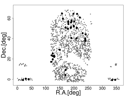
Figure 1: Projected distribution of the sub-sample of NoSOCS clusters analyzed in the present work (gray dots). Black solid circles show the random regions where the global background is computed, to check robustness of the local background determination (see § 3).

2.2 Galaxy Catalog

The galaxy catalog is obtained from the Sloan Digital Sky Survey 6th data release (hereafter SDSS-DR6), covering a total sky area of $9583\ {\rm deg}^{2}$ (Fukugita et al., 1996; Gunn et al., 1998; York et al., 2000; Adelman-McCarthy et al., 2008). For each cluster, we select all galaxies within a $10\times 10$ ${\rm Mpc}^{2}$ region, centered on the cluster centroid. The SDSS photometry of point-like sources is 95$\%$ complete down to an $r^{\prime}$-band model magnitude of ${\rm m_{r}}=22$ (Stoughton et al., 2002). Since the SDSS star/galaxy classification is still reliable down to $m_{r}\sim 21.5$ (Lupton et al. 2001; see also Capozzi et al. 2009), we select all galaxies down to the latter magnitude limit, and adopt this value as the apparent completeness magnitude $m_{c}$ of the galaxy catalog of a given cluster. This choice also ensures that there are no threshold effect when applying the K-corrections discussed below, since the completeness limit of the galaxy catalog is 0.5 mag deeper than our adopted cut. The completeness absolute magnitude of the NoSOCS sub-sample used in this work, then ranges from around $M_{c}=-16$ for the low-redshift clusters ($z\sim 0.07$), to about $M_{c}=-19$ for the upper redshift limit of $z\sim 0.2$. We retrieve only galaxies with clean photometry from SDSS, by selecting only $PRIMARY$ objects with SDSS photometry flags  set following Yasuda et al. (2001). In order to consider only regions for which the galaxy catalog has homogeneous photometric accuracy and completeness characteristics, we also exclude objects within circular regions around bright stars and large galaxies, from the Tycho-2 and RC3 catalogs (de Vaucouleurs et al., 1991), respectively. The radius $r$ of the masked regions is chosen following the prescriptions of Gal et al. (2009). For Tycho-2 stars we set ${\rm r}=2\arcmin$ for ${\rm m}_{\rm Tycho}<7.0$, ${\rm r}=1.5\arcmin$ for $7.0\leq{\rm m}_{\rm Tycho}\leq 8.0$, ${\rm r}=1.0\arcmin$ for $8.0\leq{\rm m}_{\rm Tycho}\leq 9.5$, while for galaxies in the RC3 catalog we adopt ${\rm r}=5\times{\rm r}_{\rm RC3}$ for ${\rm r}_{\rm RC3}<25\arcsec$ and ${\rm r}=8\times{\rm r}_{\rm RC3}$ for ${\rm r}_{\rm RC3}\geq 25\arcsec$.

The galaxy LF is measured in the $r^{\prime}$ band, using model galaxy magnitudes from the SDSS Photo pipeline (Lupton et al., 2001; Stoughton et al., 2002). Magnitudes are corrected for Galactic extinction according to Schlegel et al. (1998). For all galaxies in the region of a given cluster, apparent magnitudes are converted to absolute magnitudes by the relation:

$$M=m-5\log_{10}(D_{L}/10\ {\rm pc})-{\rm K}(z),$$ (1)

where D${}_{\rm L}(z)$ is the luminosity distance, and ${\rm K}(z)$ is the k-correction. In order to compute D${}_{\rm L}(z)$, we assume all galaxies in the given region to be at the same redshift as the cluster. While this is correct for cluster galaxies (considering the lower redshift limit of the NoSOCS catalog), it is certainly incorrect for foreground/background galaxies. However, the contribution of field galaxies is statically removed when computing the LF, making the computation of D${}_{\rm L}(z)$, on average, statistically correct.

In order to test the robustness of our results with respect to the method used to calculate the ${\rm K}(z)$, we adopt two independent approaches, by (i) using an average k-correction for all galaxies, and (ii) estimating a specific k-correction for each galaxy. In case (i), we adopt the k-correction for elliptical galaxies from Fukugita et al. (1995) at the cluster redshift. In case (ii), we estimate the ${\rm K}(z)$ by using the software $kcorrect$ (version $4\_1\_4$, Blanton et al. 2003), through a rest-frame filter obtained by blue-shifting the throughput curve of the SDSS r-band by a factor $(1+z_{0})$. For $z_{0}=0$, one recovers the usual k-correction. As in previous works based on SDSS data (e.g. Hogg et al. 2004), we have adopted $z_{0}=0.1$. For galaxies at redshift $z=z_{0}$, the k-correction is equal to $-2.5\log(1+z_{0})$, independent of the filter and the galaxy spectral type. Hence, since the value of $z_{0}=0.1$ is very close to the median redshift of the NoSOCS cluster catalog (see  Gal et al. 2004), this choice of $z_{0}$ allows uncertainties on k-corrections to be minimized (see Blanton et al. 2003). We run $kcorrect$ using the $ugriz$ SDSS model magnitudes, and the best estimate available for the redshift $z$ of each galaxy, i.e. either the spectroscopic redshift or the photometric estimate, when the former is not available. The two approaches have different advantages and drawbacks. In case (i), we are assuming that early-type spectral types dominate the cluster galaxy population at all magnitudes. While this is only a rough approximation, it allows us to avoid bringing the uncertainties on the k-correction of each single galaxy into the computation of the LF. On the other hand, method (ii) implies a larger uncertainty on the $K(z)$’s, but corrects each galaxy according to its proper spectral type, inferred from the photometric information. Since the foreground/background contaminants are statistically removed from the LF, both methods should be statistically insensitive to the $K(z)$ of field galaxies. Fig. 2 shows the LFs of galaxies obtained with both methods to estimate the k-correction, for two richness bins of the parent clusters. The two methods provide very similar LFs in both cases. In what follows, all results are obtained by applying method (i), but all of our results remain essentially unchanged when using method (ii).

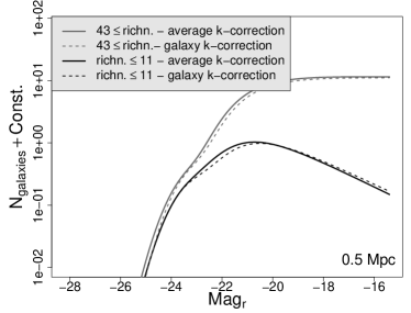
Figure 2: Best-fits LFs obtained using the the Maximum-Likelihood approach (Sec. 5.2) by applying an average k-correction value from Fukugita et al. (1995) (solid line) or k-correcting each single galaxy independently with the software $kcorrect$ (dashed line). Gray and black colors show the cases of rich and poor clusters, classified according to the richness parameter Richn._SDSS (see Sec. 2.3).

2.3 Cluster Properties

In order to analyze the environmental dependence of the LF, we derive it as a function of the richness of the parent clusters and the cluster-centric distance, obtained as follows. The optical richness of a cluster of galaxies, i.e. the number of galaxies in a given magnitude range within a given physical region of the cluster, is a proxy for its mass (Kravtsov et al., 2004; González et al., 2005; Popesso et al., 2007; Hilbert & White, 2010; Mandelbaum et al., 2010). As there is no best, objective prescription to measure the richness parameter, we have performed the analysis by using two different richness estimates.

• For each NoSOCS cluster, Gal et al. (2009) measured the richness parameter, $N_{gal}$, as the background subtracted number of galaxies in the cluster, within an aperture of $0.5\ {\rm Mpc}$, in the (r-band) magnitude range of $-22$ to $-19$. To take advantage of the more accurate SDSS photometry (relative to DPOSS), we re-measured cluster richness according to this same definition using SDSS photometry. Hereafter, this updated richness parameter is indicated as Richn._SDSS. This approach has the advantage of being simple and commonly used in the literature, as well as providing richness estimates well correlated to cluster mass (Lopes et al., 2006). However, it becomes more and more uncertain for poorer systems, as it uses only a limited range of the magnitude distribution of cluster galaxies. Notice also that the luminosity range in the definition above extends two magnitudes below $M^{\star}$, possibly introducing a spurious dependence of the LF faint-end shape on cluster richness.

• To minimize the drawbacks in the definition of Richn._SDSS, we also define a new richness estimate, Richn._ML, as the integral of the best-fitting Schechter function to the cluster LF in the luminosity range ${\rm M_{r}}\leq-21.0$. In order to account for the possible dependence of the Schechter fit on cluster richness (see § 6.1 ), we estimate Richn._ML using an iterative procedure. First, we split our cluster sample according to Richn._SDSS, and derive the Schechter fit to the LF for each richness bin. For each cluster in the bin, the LF fit is re-scaled to match the number counts of galaxies brighter than $-21$ . This provides a first richness estimate, Richn.${}^{0}_{\rm ML}$. We then re-arrange the cluster sample based on Richn.${}^{0}_{\rm ML}$, and repeat the procedure, obtaining the second, final richness estimate, Richn._ML. The Schechter function fits are obtained with the Maximum-Likelihood approach described in Sec. 5.2. Notice that this iterative procedure is preferable to measuring the Richn._ML from the Schechter fit to the LF of single clusters, since results of single fits exhibit a large measurement scatter (see §6). Richn._ML is designed to probe mainly the LF normalization at $M^{\star}$, i.e. the abundance of giant galaxies in the cluster, independent of the LF faint-end slope. On the other hand, it is based on the integral of a parametric fit re-scaled to the whole magnitude distribution of galaxies in a cluster, hence being virtually less affected by Poissonian noise on number counts with respect to richness estimates obtained by the number of galaxies in a given magnitude range. To further verify the dependence of Richn._ML on the LF faint-end slope, we simulated a set of clusters with Richn._ML ranging from 4 up to 15, i.e. the range covered by our cluster sample, and intrinsic $\alpha=-0.8$. We then recomputed Richn._ML, fitting the LF with $\alpha$ forced to be larger/smaller by 0.6 than its best-fit value, i.e. $>1\sigma$ in the large majority of cases of Table 2; this would correspond to a situation where a cluster is assigned to a completely erroneous group and thus its Richn._ML is measured using the wrong Schechter model. Even is such extreme scenario the variations in Richn._ML are less than 16% in all cases, and anyway always below the poissonian uncertainties affecting richness estimates based only on galaxy counts.

Fig. 3 compares Richn._SDSS with Richn._ML. Despite the different definitions, a good correlation is observed between the two sets of measurements. More generally, we verified that our results remain unchanged regardless of which richness estimate is used. In particular, the dependence of the LF on environment is the same using either Richn._ML or Richn._SDSS, even though in the latter case the trends reported in §6.1 appear somewhat weaker due to the reasons discussed above. For brevity, throughout the rest of the work, we will only show results obtained for Richn._ML.

Figure 3: Comparison of Richn._SDSS and Richn._ML. Notice the good correlation among the two estimates.

In order to estimate the cluster-centric distance of galaxies in different clusters, we use both fixed and, when available, characteristic radii $R_{200}$. The characteristic radius of a cluster, R₂₀₀, is the radius within which the mean inner density is $200$ times the critical density, $\rho_{c}(z)$, of the Universe at the cluster redshift. N-body simulations suggest that the bulk of the virialized mass of a cluster is generally contained within this radius (e.g. Carlberg et al., 1997). Values of R₂₀₀ were computed for a sub-sample of NoSOCS clusters from Gal et al. (2009), assuming that the radial distribution of galaxies within a cluster follows that of the dark matter, and neglecting possible variations of the mean mass of galaxies with environment. Of the $1,451$ clusters analyzed in the present work, R₂₀₀ values are available for $814$ clusters. For this sub-sample, the LFs are derived in

• three circular regions, with outer radii of $0.2\ {\rm R}_{200}$, $0.5\ {\rm R}_{200}$ and R₂₀₀, all centered on the cluster centroids;

• an outer annulus, with inner and outer radii of $0.5$ and $1$ $R_{200}$.

Deriving the LFs within regions sampling different fractions of a dynamical radius, such as $R_{200}$, rather than fixed-size apertures, can actually provide a more physically-meaningful way to compare galaxy populations at different cluster-centric radii. However, in order to fully exploit the extensive statistical power of the NoSOCS cluster sample, we also perform a fixed-aperture analysis of the LF using the entire sample of $1,451$ clusters. This also allows us to perform a more direct comparison with previous works, where $R_{200}$ measurements were not available. For the entire sample, we derive the LFs within five fixed-size apertures:

• three circular regions of radii: $0.5,\ 1.5$ and $3.0\ {\rm Mpc}$;

• two concentric annuli, with $0.5<{\rm r}\leq 1.5$ Mpc, and $1.5<{\rm r}\leq 3.0$ Mpc.

Throughout this paper, results using fixed apertures always refer to the entire cluster sample, while results within the physical apertures are obtained using the sub-sample of $814$ clusters.

3 Background Statistical Subtraction

The LF of a galaxy cluster is defined as the number of galaxies in the cluster as a function of luminosity. The primary difficulty in measuring the LF is that of assessing the membership of galaxies along the line of sight. Furthermore, projection effects tend to mimic the presence of a large population of dwarf galaxies, hence producing steep faint slopes (Valotto et al., 2001). Ideally, one would need spectroscopic redshifts for each individual galaxy in the cluster area, but this is unfeasible for a plethora of reasons. Spectroscopic measurements are extremely time demanding if possible at all: i.e. when the sample of clusters is large, when the faint end of the galaxy population has to be analyzed, when dealing with high redshift clusters. Several authors have attempted to use photometric redshifts to assess cluster membership but, even though these are effective at reducing the back/foreground contamination, the latter remains non-negligible and statistical corrections are still required to remove the contribution of contaminant sources (Tanaka et al., 2005, 2007; Rudnick et al., 2009; Capozzi et al., 2009).

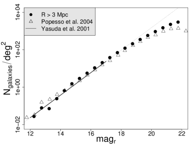
Figure 4: Top panel: Average background counts per unit area as a function of r-band magnitude (filled circles); error bars are smaller than symbols. Results from Popesso et al. (2004) (empty triangles) are also shown. The solid line plots the count-magnitude relation predicted from Yasuda et al. (2001) in the magnitude range $12\leq mag_{r}\leq 17$; the dotted line represents its extrapolation to fainter and brighter magnitudes. Bottom panels: percentage difference between local background counts per unit area, outside $3\ {\rm Mpc}$, and the: i.) local background counts outside $4\ {\rm Mpc}$; ii.) local background counts (outside $3\ {\rm Mpc}$) for the 200 poorest clusters in the NoSOCS sample; iii.) local background counts (outside $3\ {\rm Mpc}$) for the 200 richest clusters in the NoSOCS sample. iv.) global background (see the text).

The statistical background subtraction is performed by estimating the contribution of non-cluster members to the number counts of galaxies in the cluster direction, by measuring the projected number counts of field galaxies outside the cluster region. Two approaches can be used, measuring: (i) the “global” density of field galaxies on large angular areas (Gladders & Yee, 2005; Hansen et al., 2005), or (ii) the “local” background either in control fields close to the cluster, or in annuli centered on the cluster centroid (Paolillo et al., 2001; Goto et al., 2002; Popesso et al., 2005). The differences between these two methods have been extensively analyzed in the literature, with most authors finding no significant difference between them (e.g. Driver et al., 1998; Goto et al., 2002; Hansen et al., 2005; Popesso et al., 2005; Barkhouse et al., 2007). On the other hand, as noted by Paolillo et al. (2001, also see below), when one wants to isolate just the main cluster signal without analyzing the structure correlated with the cluster, the local background approach is preferable, as it takes into account possible background variations in the cluster region, caused by the large-scale structure within which the clusters are embedded.

We therefore derive the galaxy LF using a local background approach. The local background is estimated within a $10\times 10$ Mpc region, centered on the cluster centroid, outside a radius of $3\ {\rm Mpc}$ (about two times the Abell radius), where the contamination from cluster galaxies is expected to be negligible. In order to avoid over-estimating the background level because of the possible presence of back/foreground galaxy groups, we follow the approach of Paolillo et al. (2001). We generate a density map of galaxies in the background region by convolving the projected distribution of galaxies with a Gaussian kernel of $\sigma=250\ {\rm kpc}$ in the cluster rest frame (the typical size of a cluster core). Then, we mask out all density peaks, above the $3\sigma$ level, from the background region. Masked out regions cover, on average, $2-3\%$ of the whole background area and contain less than $2\%$ of all background galaxies. Clusters for which the area of the masked regions is larger than $10\%$ of the total background one are excluded from our analysis. The number counts of galaxies in the remaining region, which we call the “local background”, is adopted to estimate the expected background counts in the cluster direction, i.e. one of the regions where the LF is derived (see Sec. 2.3). Fig. 4 (top panel) shows the local background counts, per unit area, averaged among all the clusters in the NoSOCS sample. Good agreement is found with Popesso et al. (2004), who estimated background counts within randomly selected fields, and with the count-magnitude relation expected for a homogeneous galaxy distribution in a universe with Euclidean geometry, as obtained by Yasuda et al. (2001).

Fig. 4 also shows some tests we performed to check the robustness of the local background determination. The bottom panels show the fractional difference between averaged local background counts obtained outside $3\ {\rm Mpc}$ and those measured: i) outside $4\ {\rm Mpc}$; ii) outside $3\ {\rm Mpc}$ but only for the $200$ poorest clusters in the NoSOCS sample; iii) outside $3\ {\rm Mpc}$ but only for the $200$ richest clusters. Panels i.–iii. show no appreciable difference ($<1\%$, on average) in number counts in the two background regions, implying that, on average, we are not overestimating the background counts, as might be the case if some residual signal from the cluster would be still detectable in our “local” background. If present, such effect would indeed be less important at larger cluster-centric distances (panel i.), and/or produce a fictitious higher background level for richer clusters (panel iii.), while no measurable difference is instead observed. Sheldon et al. (2009), in their weak lensing analysis, measure the excess number density due to the cluster in the background region to vary between $\sim 1\%$ for poorest groups to $\sim 3.5\%$ for rich clusters. Poorest groups are excluded from our cluster sample, and hence the difference in the excess number densities caused by poor and rich clusters in the surrounding background region should be lower than $\sim 2.5\%$, measured over the whole magnitude range, in rough agreement with what found in this work.

As a further test, we also extracted a “global” background from $42$ control fields, selected within the SDSS area, containing no known galaxy clusters. The control fields have a radius of $60\arcmin$ each, covering a total area of $\approx 130\ {\rm deg}^{2}$. Their distribution on the sky is shown in Fig. 1 (black solid circles). The difference between the counts measured in this “global” background, and those obtained in the “local“ one (outside $3\ {\rm Mpc}$), is plotted in panel iv. of Fig. 4. While for bright magnitudes, $m_{r}<14$, the two background estimates are consistent within the errors, the global background tends to be systematically lower than the local one for fainter magnitudes, in agreement with the findings of Paolillo et al. (2001). Since we can reasonably exclude that our background local estimate is over-estimated because of contamination from cluster galaxies (see panel i. in Fig. 4), we can conclude that the local background also includes the contribution of the large-scale structure around clusters and groups of galaxies, which is instead not accounted for by the number counts in the control fields. Throughout the present work we then compute the LFs by using the local rather global background determination. We note that, while many authors have claimed no significant differences in the LF when using either the local or global background, Fig. 4 of Popesso et al. (2004) reveals, in agreement with our findings, a tendency for the LF to have a shallower faint-end slope when using global background counts, implying a differential slope between the local and global background galaxy counts, which could affect the slope of the faint-end slope of the resulting LF.

4 Individual Luminosity Functions

In order to derive the LF of galaxies in individual NoSOCS clusters, for each cluster we estimate the number counts of galaxies in the local background region (see previous section) and subtract them from the number counts of galaxies in the cluster region (see § 2.3). Number counts are computed in half-magnitude bins. Background counts are rescaled to the effective area of the cluster region, accounting for excised areas due to bright objects in both background and cluster regions (§ 2.2). Errors on the individual LFs are measured following Paolillo et al. (2001).

As an example of the procedure to derive the single LFs, Fig. 5 exhibits background and cluster number counts, as well as the resulting LF for two clusters among the poorest (NSC14787, ${\rm z=0.132}$, top panels) and richest (NSC09718, ${\rm z=0.137}$, bottom panels) structures in the NoSOCS sample. While for rich structures the LF is significantly detected above the background level, poor structures are affected by their very low density contrast, as shown by the large uncertainties on background-subtracted number counts at both the bright and faint ends of the LF.

Figure 5: Left panels. Galaxy counts extracted within R200 (solid circles), and in the local background (empty circles) for the poor cluster NSC14787 (top) and rich cluster NSC09718 (bottom), both located at ${\rm z\approx 0.13}$. Right panels. Background subtracted number counts, i.e. individual LFs, of the two clusters. The dashed line corresponds to the completeness limit of the SDSS photometry (Sec. 2.2); the solid line shows the best fit models. Poor structures, with low signal LFs, might lead to unrealistic results in the LF best fit (as for NSC14787, top right panel), which cause the large spread in the LF results, shown in Fig. 9.

In order to characterize the properties of the individual LFs, we fit them by a parametric model given by the Schechter function:

$$\Phi(M)dM=\Phi^{*}\ 10^{0.4(M^{*}-M)(\alpha+1)}\exp\left(10^{0.4(M^{*}-M)}\right)dM$$ (2)

where $M$ is the galaxy magnitude, $\Phi^{*}$ is the normalization factor, $M^{*}$ is the characteristic knee magnitude and $\alpha$ is the faint-end slope of the LF. For each cluster, we fit the background-subtracted counts using a $\chi^{2}$ minimization procedure. To calculate the $\chi^{2}$, the LF model is integrated over each magnitude bin. Uncertainties on the best-fitting parameters, $\Phi^{*}$, $M^{*}$, and $\alpha$, are determined by marginalizing each parameter over the remaining ones. Results are presented in Sec. 6.

5 Composite Luminosity Functions

To analyze the dependence of the cluster LF on different properties, such as cluster richness, redshift, and cluster-centric distance of galaxy populations, we bin the NoSOCS sample with respect to each quantity, and derive the composite LF of galaxies in each bin. The composite LFs are derived using two alternative approaches: by performing a weighted average of the individual cluster LFs (Sec. 5.1), and by performing a simultaneous Maximum-Likelihood (hereafter ML) fit to all the individual cluster LFs in the given bin (Sec. 5.2). The first approach is non-parametric, i.e. we make no prior assumptions on the shape of the LF, while the ML fit assumes a given functional form.

5.1 Non-parametric Approach: “cumulating” the LF

The cumulative LF (hereafter CLF) of a given sample of galaxy clusters is the weighted mean of the individual LFs. Previous works have focused on the differences among alternative cumulation approaches, and the following two methods have come out as the most reliable ones:

Colless method.

Colless (1989) derived the CLF as:

$$N_{\rm cj}=\frac{N_{\rm c0}}{m_{\rm j}}\sum_{i}\frac{N_{\rm ij}}{N_{\rm i0}},$$ (3)

where $N_{\rm cj}$ is the number of galaxies in the $j$-th bin of the CLF, ${N_{\rm ij}}$ is the number of galaxies in the $j$-th bin of the $i$-th cluster LF, $m_{j}$ is the number of clusters contributing to the $j$-th magnitude bin, ${N_{\rm i0}}$ is a normalization factor and:

$$N_{\rm c0}=\sum{N_{\rm i0}}.$$ (4)

For the $i$-th cluster, the ${N_{\rm i0}}$ is defined as the number of galaxies brighter than the completeness absolute magnitude, $M_{c}$, of the cluster sample. For a flux-limited survey, $M_{c}$ coincides with the completeness magnitude of the most distant cluster. The error on the resulting CLF is

$$\sigma_{N_{\rm cj}}=\frac{N_{\rm c0}}{m_{\rm j}}\sqrt{\sum_{i}\left(\frac{\sigma_{N_{\rm ij}}}{N_{\rm i0}}\right)^{2}},$$ (5)

where $\sigma_{N_{\rm ij}}$ is the statistical uncertainty on $N_{\rm ij}$ (see Sec. 4). For the NoSOCS sample, we compute the individual LFs as described in Sec. 4. The completeness magnitude of the sample is $M_{c}=-19$ in the $r^{\prime}$ band (see Sec. 2.2), and ${N_{\rm i0}}$ is hence computed as the field-corrected number of galaxies, of the $i$-th cluster, brighter than $-19$.

GMA method.

Garilli et al. (1999) proposed an alternative cumulation method, where one weights each cluster LF according to the number of galaxies contained within an adaptive magnitude range. In this approach, the CLF is given by:

$$N_{\rm cj}=\frac{1}{m^{\prime}_{\rm j}}\sum_{i}N_{\rm ij}w_{\rm i}^{-1}$$ (6)

where $N_{\rm cj}$ and $N_{\rm ij}$ are defined as in the Colless method, $m^{\prime}_{\rm j}$ is the number of clusters with completeness magnitude fainter than the $j$-th bin, and $w_{\rm i}$ is the normalization factor of each cluster. For the $i$-th cluster, we denote as $M_{c,i}$ its completeness (absolute) magnitude. The $w_{\rm i}$ is given by the ratio of the number of galaxies brighter than $M_{c,i}$ in the cluster, to the average number of galaxies brighter than $M_{c,i}$ among all clusters whose completeness magnitude goes fainter than $M_{c,i}$. The error on the CLF is

$$\sigma_{N_{\rm cj}}=\frac{1}{m^{\prime}_{\rm j}}\sqrt{\sum_{i}\left(\sigma_{N_{\rm ij}}w_{\rm i}^{-1}\right)^{2}},$$ (7)

where $\sigma_{N_{\rm ij}}$ is defined as for the Colless method.

The main difference between the two cumulation methods is that Colless weights each LF by the number of galaxies in a fixed magnitude range, while the GMA takes advantage of the different completeness magnitude of each cluster, hence fully exploiting all the available information in the data. In principle, both methods should provide identical results, at least as far as all clusters exhibit, in a statistical sense, the same LF, i.e. the cluster LF is $``universal^{\prime\prime}$. Fig. 6 compares the CLFs obtained by the two methods for all NoSOCS clusters within a region of radius $0.5\ {\rm Mpc}$. The methods agree very well on the bright end of the LF, while at faint magnitudes, we see a trend for the Colless method to produce a steeper faint-end than that of the GMA CLF. A trend in the same direction has been already reported by Popesso et al. (2005) (hereafter P05), who detected a dramatic drop-off in the CLF faint-end when using the GMA, rather than Colless, method. P05 explained this effect as a result of a strong correlation among the GMA weights, $w_{i}$, and the completeness magnitude M_c,i of the clusters. This would actually lead to down-weighting the LFs of clusters having a deeper completeness magnitude hence producing a sharp decline in the CLF faint end. Fig. 7 plots the GMA weights for the NoSOCS sample as a function of the cluster completeness magnitude, $M_{c,i}$. In contrast to P05, we find no strong correlation between $w_{i}$ and $M_{c,i}$ (cfr Fig. 5 of P05), implying that the difference between Colless and GMA CLFs is not caused by the trend found by P05 .

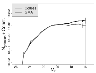
Figure 6: Composite LFs (within the cluster region of radius $0.5\ {\rm Mpc}$) obtained applying the Colless and GMA methods plotted, respectively, as black and gray solid lines.

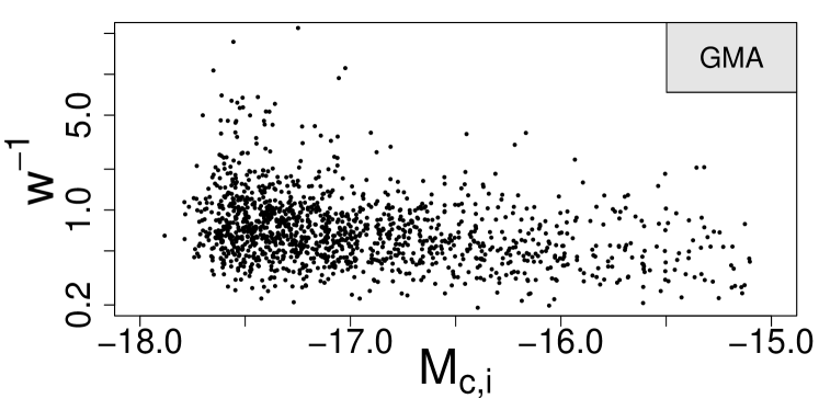
Figure 7: Dependence of the GMA weight, w_i, on the completeness magnitude, $M_{c,i}$, of NoSOCS clusters. Notice that no relevant correlation is detected.

The difference between the Colless and GMA methods is instead related to the fact that the GMA computes the weights by also counting galaxies in the faint end of the individual LFs. In the case where the bright part of the LF is identical for all clusters in the sample, all of the individual LFs have the same weight in the Colless method, regardless of the shape of the faint-end slope. For the GMA, the $w_{i}$’s are the same only if the faint-end part of the LFs is the same for all clusters. If this is not the case, clusters with a steeper faint-end have a smaller $w_{i}^{-1}$, i.e. are down-weighted in the CLF (see Eq. 6). In other words, if the individual cluster LFs have different faint-end slopes, the GMA will give more weight to those clusters with a shallower LF faint-end, hence producing the difference between the two CLFs, as observed in Fig. 6. The variation of the faint-end slope among clusters can be either (i) intrinsic, i.e. the LF is not universal, or (ii) statistical, because of the non-Poissonian background fluctuation on the cluster angular scale (see Sec. 3). Poissonian uncertainties (on both cluster and field counts) do not alter the shape of the individual cluster LF, as the errors on different magnitudes are not correlated. This is not the case for the non-Poissonian contribution to the error budget. As shown in Sec. 6, point (i) is certainly important in driving the difference of the CLFs from the two methods in Fig. 6, as the LF faint-end slope turns out to depend significantly on cluster richness.

While both the GMA and the Colless methods have the advantage of being non-parametric, they are also significantly affected by statistical fluctuations in the individual LFs, in particular when the individual LFs have low S/N ratio, i.e. for poor groups and for the outskirt regions of clusters, as well as at the extreme faint end of the LF. At faint magnitudes, statistical fluctuations in the background signal can even lead to negative values of field-corrected number counts of the individual LFs, possibly making the weighted mean in Eq. 3 and Eq. 6 ill-defined. The GMA method is more sensitive to this issue than the Colless one, as the weight for each LF is computed by including also the faint range of the LF, where background fluctuations are more important. Therefore, while both cumulation methods can be applied straightforwardly to well controlled samples of rich structures, caution should be taken when analyzing individual LFs with a variety of S/N ratios and completeness limits.

5.2 Parametric Approach: the Maximum Likelihood Technique

An alternative approach to derive the composite LF of a cluster sample is to perform a simultaneous Maximum Likelihood fit of number counts for all clusters. While this method has the drawback of being parametric, in that a given analytic functional form of the global LF has to be assumed, it has several advantages relative to the cumulative approach. First, the data are not binned. Second, no correction has to be applied for incompleteness at the faint end, and third, it is not affected by the issue of negative values of field-subtracted number counts.

The ML approach and its advantages have been thoroughly described by Andreon et al. (2005); henceforth we shortly describe only its implementation for the analysis of the NoSOCS sample. First, we have to adopt a given functional form for the global LF. As noted in Sec. 4, a single Schechter function provides a reasonable tool to analyze the LF of individual clusters, where the uncertainties on number counts usually do not allow a detailed analysis of the shape of the LF. Now instead we consider a Schechter plus a Log-normal function. The latter term is used to describe the LF of Brightest Cluster galaxies (BCGs), which are known not to follow the Schechter distribution typical of faint galaxies (Thompson & Gregory, 1993; Biviano et al., 1995; Hansen et al., 2009).

To perform the ML fits, we assume that each galaxy is extracted from a probability distribution consisting of the above model plus a second order power-law, representing the background component. For each cluster, we first fit the second order power-law to the local background. The best fit is rescaled to the angular area of the cluster region. Galaxy counts in all the cluster regions are then fitted simultaneously, by keeping fixed, for each cluster, its rescaled background power-law component . The fitting parameters are the characteristic magnitude, $M^{\star}$ and the faint-end slope, $\alpha$, of the Schechter function, the central magnitude, $M^{\star}_{BCG}$, and width, $\sigma_{BCG}$, of the BCG’s component, and the two normalization factors of the Schechter and log-normal functions.

The normalization factors are let free to vary from cluster to cluster, while the other parameters are set to have the same values for all clusters. The ML fits are performed using the L-BFGS algorithm as for the fitting of the individual LFs (Sec. 4). L-BFGS is well suited for optimization problems with a large number of dimensions, as is the case for the CLF fitting, because it never explicitly forms or stores the Hessian matrix (Lu et al., 1994), still allowing upper and lower constraints for each variable to be measured. We also constrain the fitting parameters of the log-normal component of the CLF to be in the range of $-23.5\leq M^{\star}_{BCG}\leq-22.5$ and $0.3\leq\sigma_{BCG}\leq 1.0$, based on the typical range spanned by BCGs (e.g. cf Hansen et al., 2009). Confidence limits are evaluated by marginalizing over all unwanted free parameters.

6 Results and Discussion

The measurement of the LF of galaxy clusters is an intrinsically multiparametric problem. Local and global galaxy density, density of the intra-cluster medium, age etc. are all known to affect the relative balance between galaxy populations in clusters through several effects such as merging, tidal stripping, harassment, ram pressure stripping and strangulation, whose interplay is not yet well understood.

We have underlined in the previous sections that the assumption of a universal LF shape in samples spanning a large range of parameters and S/N, is not merely an approximation which hides the details of the processes at work, but may produce biases in the final results altering the measured LF parameters depending on the technique used to weight the individual LFs.

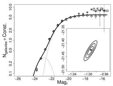
Figure 8: ML fit obtained using a Schechter plus a Log-normal components (solid line). The individual components are shown as dashed lines. Data were extracted within $0.5\ {\rm R}_{200}$. Confidence levels for the free parameters of the Schechter function are also plotted. Gray circles and empty diamonds represent the composite LFs obtained using the Colless and GMA methods, respectively.

Table 1: Results ML fit within $0.5\ {\rm R}_{200}$.

$\alpha$	$M^{\star}$
$-0.99_{-0.02}^{+0.01}$	$-21.42_{-0.04}^{+0.03}$

Nevertheless, in order to allow a comparison with previous studies of large cluster samples, we derived a “global” LF of the overall sample within $0.5\ {\rm R}_{200}$ (see Fig.8 and Table  1). Differences in cumulation techniques, extraction radii and richness of the samples affect the shape of the LF (see $\S$ 5.1 and § 6.1), making a comparison between independent works a difficult task.

In general, the $M^{\star}$ values agree very well within the uncertainties among different authors, while the faint-end slope of the LF is more debated. Once the different pass-bands and cosmologies are taken into account, our $M^{\star}$ is indeed in fair agreement with Crawford et al. (2009); Garilli et al. (1999); Paolillo et al. (2001), with Yang et al. (2009) for galaxy groups in the SDSS, and with Rudnick et al. (2009) for red-sequence galaxies, which dominate the bright end of the LF.

For the steepness of the faint end, our results are in good agreement with the X-ray selected clusters by Valotto et al. (2004) ($\alpha=0.9\pm 0.1$), and in marginal agreement with Paolillo et al. (2001) ($\alpha=1.11^{+0.09}_{-0.07}$). The slightly steeper faint end measured by Paolillo et al. (2001) is probably an effect of both the larger extraction radius (${\rm r}\sim 2\ {\rm Mpc}$) and the sample of rich Abell clusters used. Trends for flatter faint end slopes are instead observed by Garilli et al. (1999); Crawford et al. (2009) ($\alpha=-0.81^{+0.05}_{-0.10}$ and $\alpha=-0.84\pm 0.32$, respectively). While the average value of $\alpha$ measured by Crawford et al. (2009) over the whole low-redshift cluster sample is consistent with our findings within the uncertainties, the difference with Garilli et al. (1999) can be attributed to their smaller extraction radius ($<{\rm r}>\sim 250\ {\rm kpc}$).

Hansen et al. (2005, 2009), fitting a MaxBCG selected sample down to $M_{r}<-19$, derive a shallower faint-end. The latter sample however may be skewed toward poorer systems with respect to NoSOCS, since when differentiating according to cluster richness their results are in much better agreement with ours (see 6.1).

On the other hand, while their $M^{\star}$ are typically $>0.6~{}{\rm mag}$ dimmer, their cluster finding technique might favor systems whose LF exhibits a prominent BCG component, resulting in a pronounced Log-normal component at the bright end, which is not observed in our sample . We speculate that the presence of a more prominent Log-normal component anti-correlates with the LF characteristic magnitude, in the sense that systems with a stronger Log-normal component have dimmer satellites.

Popesso et al. (2005) find a steeper faint end and brighter $M^{\star}$ ($\alpha=-1.33\pm 0.06$, $M^{\star}=-22.17\pm 0.20$ within $1\ {\rm Mpc}\ {\rm h}^{-1}_{100}$) than we do, but their results strongly vary depending on the extraction region that they use. Their two-component fit within both $1.0\ {\rm Mpc}\ {\rm h}^{-1}_{100}$ and $2.0\ {\rm Mpc}\ {\rm h}^{-1}_{100}$ is in fact roughly consistent with our $\alpha$ value ($\alpha=-1.05\pm 0.13$ and $\alpha=-1.03\pm 0.14$, respectively), while they observe a much shallower trend within $1.5\ {\rm Mpc}\ {\rm h}^{-1}_{100}$ ($\alpha=-0.76\pm 0.13$). When comparing LFs extracted within the same physical radius R₂₀₀, the steepness of the best-fit bright Schechter component from a later work by the same authors (Popesso et al., 2006) is instead in agreement with our findings ($\alpha=-1.09\pm 0.09$, while we measure $\alpha=-1.15\pm 0.02$ over the whole R₂₀₀ sub-sample); their characteristic magnitude is only slightly brighter than our measured value ($M^{\star}=-21.71\pm 0.16$ against $M^{\star}=-21.43\pm 0.6$). At the faintest magnitudes ($M_{r}\lse-18$) Popesso et al. (2006) detect a significant upturn which is not seen in our data (see Fig. 6). However, we do not probe magnitudes fainter that $M_{r}<-16$; also note that these authors adopted the Colless cumulation approach which can result in a steeper LF, in particular when the sample is weighted using only galaxies much brighter than the cumulative LF limit ($\S$ 5.1).

Valotto et al. (2004) find that artificially steep faint end slopes might be caused by projection effects resulting from background galaxies, which cannot be corrected for by subtracting background fields for 2d selected clusters with no significant 3d counterpart. Despite the 2d selection algorithm applied to compile the NoSOCS catalogue, the reality of NoSOCS clusters was verified both by photometric redshifts and by X-ray analysis of a sub-sample of NoSOCS clusters (Lopes et al., 2006). In any case, we do not observe the steep LF faint end described by Valotto et al. (2004).

In Fig. 9 we plot the results of the individual best-fits to all clusters within 0.5 R₂₀₀. The individual LFs show a wide scatter, due to the combined effects of variable S/N levels (un-physical results are obtained for many low S/N ratio or very bright completeness limit systems) and intrinsically different galaxy populations (see $\S$ 6.1). Despite this, the most likely values within the whole sample are in excellent agreement with the best fit of the ML fit obtained using a single Schechter function (plotted as a white circle).

In the following sections we split our sample in sub-samples of clusters spanning small ranges of richness, cluster-centric distance and redshift in order to minimize cumulation biases and understand the main parameters driving galaxy evolution in different environments.

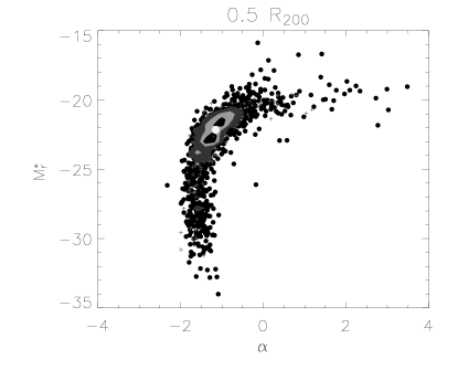
Figure 9: Results of the individual fit to a single Schechter function for all clusters in our sample within $0.5\ {\rm R}_{200}$. Rich clusters (Richn${}_{\rm ML}\geq 9$) are plotted as gray crosses; all other clusters are shown as black dots. Over-plotted are the contours including $25\%$, $50\%$ and $75\%$ of the whole distribution. A white dot shows the result of the ML best fit obtained using a single Schechter function.

6.1 LF Dependence on the Environment

Discordant results have been reported in literature in the past years, about $M^{*}$ being brighter in clusters than in the field, with an increasing trend for higher mass-systems (De Propris et al., 2003; Hansen et al., 2009; Barkhouse et al., 2007, 2009; Crawford et al., 2009). This is in agreement with hierarchical models for galaxy formation and evolution, where the frequency of mergers increases in intermediate and high mass systems, such as rich groups and clusters, causing galaxies in structures to be typically brighter than in the field, hence resulting in a brighter M*.

Substantial differences in the shape of the LF at different selection radii have been found for clusters at both low (Barkhouse et al., 2007; Popesso et al., 2006; Lobo et al., 1997; Robotham et al., 2010) and moderate-to-high redshift (Crawford et al., 2009). While the slopes of the LFs are similar at bright magnitudes, the main differences arise at the faint end where the influence of the dwarf galaxies causes an increase in the steepness of $\alpha$ with cluster-centric distance. The sampling depth and the effective cluster-centric distance thus have a great influence on the measured shape of the LF since the inclusion of different fractions of the dwarf galaxy population will directly impact the slope of the faint end. Similar results have also been reported for field galaxies (Xia et al., 2006). On the other hand, a lack of significant trends with cluster-centric radius, has also been reported (Hansen et al., 2009) although limited to brighter magnitudes (Rudnick et al., 2009). A dependence of the faint-end slope on the mass of the cluster has also been reported, suggesting that more massive clusters exhibit higher dwarf to giant ratios than less massive ones (De Lucia et al., 2004; Zandivarez et al., 2006; Gilbank et al., 2008).

We start by splitting our sample into five equally populated sub-sets of fixed richness ranges. The top left panels of Figs. 10 and 11 show the ML fit for the LFs in all richness bins, within a projected radius of $0.5{\rm Mpc}$ and $0.5{\rm R}_{200}$, respectively. Both panels reveal a systematic change of the overall population across the five richness bins, in the sense that the lowest multiplicity bins show strong dwarf suppression and fainter M^∗. We note that the decreasing relative normalization of the LFs is real, a result of the decreasing cluster richness.

To explore the influence of the extraction region and of the cluster-centric distance we fit the LFs within several extraction radii (both fixed and physical) for each richness sub-sample: an outer annulus ($0.5\ {\rm R}_{200}\leq{\rm R}\leq{\rm R}_{200}$ and $0.5\ {\rm Mpc}\leq{\rm R}\leq 1.5\ {\rm Mpc}$, for the physical and fixed apertures, respectively) and a larger projected radius (${\rm R}\leq{\rm R}_{200}$ and ${\rm R}\leq 1.5\ {\rm Mpc}$). Results of the ML fits are listed in Table 2 and shown in the bottom and top right panels in Figs. 10 and 11.

At larger cluster-centric radii (top right panels) we observe that the faint end slope becomes systematically steeper for all richness bins, respect to what observed within smaller apertures ($0.5{\rm Mpc}$ and $0.5{\rm R}_{200}$), while no dramatic change is observed on the bright side. Furthermore, the dependence on richness both of the steepness of the faint end and of the characteristic magnitude, is very diluted. Eventually, the bottom panels show that in the outer annuli clusters maintain a similar shape, within their $3\sigma$ errors, among all richness bins. This reveals that the sharp steepening of the faint-end and the M^∗ brightening with richness, observed out to large projected radii, is mainly due to the galaxies located within the central cluster regions. Outside $\sim 0.5\ {\rm R}_{200}$ cluster galaxies appear to share similar LFs, regardless of the mass of the parent halo mass. It is thus likely that studies using large apertures, either physical or fixed, are unable to identify such trends due to the role played by the central cluster regions in determining the LF shape. Similar results are observed at all scales: from galaxy groups (Robotham et al., 2010) to rich clusters (Popesso et al., 2006).

The decrease of the relative number of dwarf galaxies towards the cluster center is most probably not due to recent merging processes, since these are inhibited by the high velocity dispersions in cluster cores. Also, we observe that the shape of the bright end does not strongly depend on environment; bright early-type cannot hence be the product of cluster environment. The most likely explanations for these massive galaxies is tidal collisions or collisional disruption of the dwarfs, which most probably ends-up contributing to the intra-cluster diffuse light.

We point out that the normalization of the Log-normal component is poorly constrained in our fits especially for poor systems, since it is individually measured for each cluster. A more detailed analysis of the bright galaxy population is thus deferred to a future work.

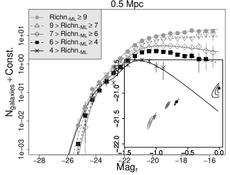
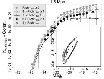
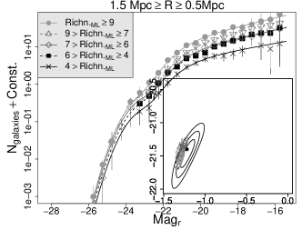
Figure 10: ML fit of the LFs extracted within $0.5\ {\rm Mpc}$, $1.5\ {\rm Mpc}$, and for $0.5\ {\rm Mpc}<{\rm R}\leq 1.5$ Mpc in bins of increasing richness. Relative confidence levels are also plotted. Results are for Richn._ML richness estimates. Data points show the composite LFs obtained using the GMA approach.

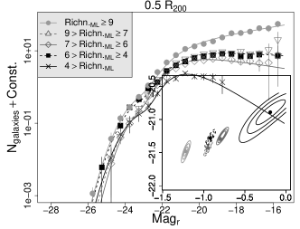
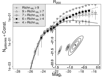
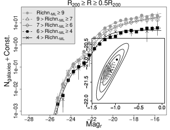
Figure 11: ML fit of the LFs extracted within $0.5\ {\rm R}_{200}$, $R_{200}$ and for $0.5\ {\rm R}_{200}<{\rm R}\leq{\rm R}_{200}$ in bins of increasing richness. Relative confidence levels are also plotted. Results are for Richn._ML richness estimates. Data points show the composite LFs obtained using the GMA approach.

Table 2: Results of the ML fit of the LFs extracted with different extraction radii in bins of increasing richness. Results are for Richn._ML richness estimates.

	Richn.${}_{\rm ML}<4$	$4\leq{\rm Richn}_{\rm ML}<6$	$6\leq{\rm Richn}_{\rm ML}<7$	$7\leq{\rm Richn}_{\rm ML}<9$	$9\leq{\rm Richn}_{\rm ML}$
R$\leq 0.5\ {\rm Mpc}$
$\alpha$	$-0.01_{-0.01}^{+0.11}$	$-0.68_{-0.04}^{+0.04}$	$-0.82_{-0.04}^{+0.04}$	$-1.03_{-0.08}^{+0.07}$	$-1.10_{-0.04}^{+0.05}$
M∗	$-20.90_{-0.18}^{+0.12}$	$-21.17_{-0.05}^{+0.06}$	$-21.23_{-0.07}^{+0.07}$	$-21.46_{-0.14}^{+0.16}$	$-21.58_{-0.13}^{+0.13}$
R$\leq 1.5\ {\rm Mpc}$
$\alpha$	$-0.9_{-0.4}^{+0.2}$	$-1.15_{-0.07}^{+0.08}$	$-1.17_{-0.05}^{+0.05}$	$-1.24_{-0.05}^{+0.06}$	$-1.25_{-0.04}^{+0.04}$
M∗	$-21.0_{-2.0}^{+1.1}$	$-21.47_{-0.18}^{+0.19}$	$-21.39_{-0.14}^{+0.12}$	$-21.46_{-0.15}^{+0.15}$	$-21.56_{-0.14}^{+0.10}$
$0.5\ {\rm Mpc}\leq$ R $\leq 1.5\ {\rm Mpc}$
$\alpha$	$-1.22_{-0.18}^{+0.21}$	$-1.30_{-0.06}^{+0.06}$	$-1.26_{-0.08}^{+0.05}$	$-1.29_{-0.07}^{+0.04}$	$-1.29_{-0.05}^{+0.04}$
M∗	$-21.4_{-0.5}^{+0.4}$	$-21.5_{-0.2}^{+0.2}$	$-21.37_{-0.17}^{+0.15}$	$-21.34_{-0.21}^{+0.11}$	$-21.54_{-0.17}^{+0.14}$
R$\leq 0.5\ {\rm R}_{200}$
$\alpha$	$-0.2_{-0.4}^{+0.2}$	$-0.92_{-0.06}^{+0.07}$	$-0.80_{-0.04}^{+0.10}$	$-0.95_{-0.05}^{+0.06}$	$-1.22_{-0.05}^{+0.06}$
M∗	$-20.9_{-0.4}^{+0.3}$	$-21.28_{-0.14}^{+0.13}$	$-21.29_{-0.09}^{+0.18}$	$-21.43_{-0.12}^{+0.11}$	$-21.48_{-0.17}^{+0.16}$
R$\leq{\rm R}_{200}$
$\alpha$	$-0.8_{-0.2}^{+0.3}$	$-1.38_{-0.06}^{+0.05}$	$-1.06_{-0.07}^{+0.07}$	$-1.08_{-0.08}^{+0.05}$	$-1.32_{-0.08}^{+0.04}$
M∗	$-21.2_{-0.5}^{+0.4}$	$-21.46_{-0.17}^{+0.13}$	$-21.29_{-0.17}^{+0.16}$	$-21.25_{-0.19}^{+0.10}$	$-21.30_{-0.28}^{+0.08}$
$0.5\ {\rm R}_{200}\leq$R$\leq{\rm R}_{200}$
$\alpha$	$-1.0_{-0.4}^{+0.3}$	$-1.11_{-0.10}^{+0.10}$	$-1.22_{-0.10}^{+0.08}$	$-1.15_{-0.08}^{+0.10}$	$-1.18_{-0.09}^{+0.09}$
M∗	$-20.9_{-1.0}^{+0.4}$	$-21.2_{-0.2}^{+0.2}$	$-21.2_{-0.3}^{+0.2}$	$-21.1_{-0.2}^{+0.2}$	$-21.3_{-0.2}^{+0.3}$

6.2 Redshift Evolution

The NoSOCS sample studied in this work spans only a limited range of redshifts ($0.07\leq z<0.2$). In order to study the evolution of the LF within this limited redshift range, we thus need to control the effects due to richness and extraction radii discussed in the previous section, which may otherwise dominate possible LF variations. We hence divide our sample into rich (${\rm Richn.}_{\rm ML}\geq 6$) and poor (${\rm Richn.}_{\rm ML}<6$) clusters in order to minimize the intrinsic variation of the LF shape (see § 6.1). We further limit the analysis to the central $0.5\ {\rm Mpc}$, where we have observed the strongest dependence of the galaxy population with the environment (see § 6.1). We then analyze three redshift bins $0.07\leq z<0.11$, $0.11\leq z<0.18$ and $0.18\leq z<0.2$, chosen to maximize the separation between high and low-z systems, while still retaining a significant number of clusters in each group.

Fig. 12 presents the LFs derived for the three redshift bins. We find a clear indication that the dwarf to giant ratio increases with decreasing redshift, both for rich and poor systems. This confirms results (of varying significance) already reported in literature (Kodama et al., 2004; Goto et al., 2005; Tanaka et al., 2005; Stott et al., 2007; Crawford et al., 2009) for cluster samples spanning much wider redshift ranges. Similar trends have also been reported for field galaxies (Willmer et al., 2006; Xia et al., 2006; Ryan et al., 2007). We underline that the above result might be affected by the decrease in completeness limit as a function of redshift. We measure this effect by fitting data in the lowest redshift bin, using the completeness limit of the highest bin. We indeed observe a decrease in the steepness of the faint end ($\alpha=-1.06_{-0.05}^{+0.06}$ for $6\leq{\rm Richn.}_{\rm ML}$), but still significantly different from what measured in the highest redshift objects of our sample (see Table 3). It is also true that the cluster catalog completeness, as a function of redshift, must be taken into account in order to draw conclusions about the LF evolution with lookback time. The completeness of the NoSOCS catalog has been tested through extensive mock cluster simulations, as discussed in Gal et al. (2009): the catalogue is $>80\%$ complete over the redshift range explored here for rich clusters, while for poor systems the completeness is a strong function of redshift, dropping below 50% at $z>1.5$ (see e.g. Figs. 4, 5 and 6 of Gal et al., 2003, for details). Finding the same redshift evolution in $\alpha$ in both rich and poor clusters thus strengthens our conclusions since the former are less subject to completeness bias due to the NoSOCS catalog, than the latter ones. Furthermore, any NoSOCS completeness effect would result in a steepening of the faint end at high redshift, since the sample there would be dominated by rich systems which have a steeper faint-end slope than rich ones (Figures 10 and 11). In this respect our result must be considered a conservative estimate of the LF dependence on lookback time.

We further measure a trend for stronger suppression of faint galaxies (below M${}^{*}+2$) with increasing redshift in poor systems, with respect to more massive ones, indicating that the evolutionary stage of less massive galaxies depends more critically on the environment. A similar trend has been observed for faint red galaxies by Koyama et al. (2007), while discordant results are instead found by Crawford et al. (2009); Andreon (2008).

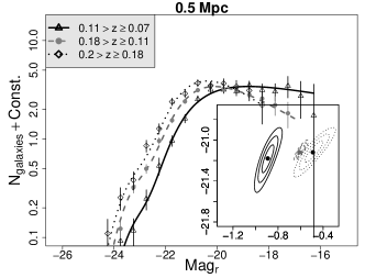
Figure 12: Left panel: ML fit of the LFs (extracted within $0.5\ {\rm Mpc}$) of the richest structures (${\rm Richn.}_{\rm ML}>6$), split into three redshift bins, together with relative contours, corresponding to the significance levels of 1 2 and 3 $\sigma$. Right panel: same as left panel, but for the poorest structures (${\rm Richn.}_{\rm ML}<6$).

Table 3: Results of the ML fit (within a projected radius of $0.5\ {\rm Mpc}$ splitting our sample by redshift at $z=0.10$ and $z=0.17$ for both the richest ($6\leq{\rm Richn.}_{\rm ML}$) and poorest ($4\leq{\rm Richn.}_{\rm ML}<6$) clusters.

	$0.07\leq{\rm z}<0.11$	$0.11\leq{\rm z}<0.18$	$0.18\leq{\rm z}<0.2$
$6\leq{\rm Richn.}_{\rm ML}$
$\alpha$	$-1.19_{-0.05}^{+0.04}$	$-0.98_{-0.02}^{+0.02}$	$-0.85_{-0.05}^{+0.07}$
M∗	$-21.6_{-0.2}^{+0.2}$	$-21.34_{-0.05}^{+0.05}$	$-21.33_{-0.09}^{+0.12}$
$4\leq{\rm Richn.}_{\rm ML}<6$
$\alpha$	$-0.89_{-0.12}^{+0.13}$	$-0.61_{-0.05}^{+0.08}$	$-0.5_{-0.2}^{+0.2}$
M∗	$-21.2_{-0.3}^{+0.4}$	$-21.12_{-0.08}^{+0.12}$	$-21.1_{-0.3}^{+0.2}$

7 Conclusions

We presented the analysis of the Luminosity Function of galaxy clusters from the Northern Sky Optical Cluster Survey, using $r^{\prime}$-band data from the Sloan Digital Sky Survey. The sample, including 1451 galaxy groups and clusters, is large enough to allow us to investigate in detail both the intrinsic differences in the galaxy populations as a function of richness, cluster-centric distance and redshift, as well as the uncertainties introduced by different analysis techniques commonly used in the literature.

Our global LF agrees with previous studies of galaxy clusters and does not show the presence of an “upturn” at faint magnitudes down to $M_{r}\lse-16$, presented by some earlier works as the proof of the presence of a very large population of dwarf galaxies (e.g. Popesso et al., 2005; González et al., 2006).

We do observe a strong dependence of the LF shape ($M^{\star}$ and faint-end slope) on both richness and extraction radius as expected from the morphology-density relation and most physical models of galaxy evolution in dense/massive systems. The dwarf to giant ratio increases with richness, indicating that more massive systems are more efficient in creating/retaining a population of dwarf satellites. Furthermore, in the innermost regions $R\leq 0.5\ {\rm R}_{200}$ we observe a sharp steepening of the faint-end and an M^∗ brightening with richness. The same effect is observed both within fixed ($0.5\ {\rm Mpc}$) and physical ($0.5\ {\rm R}_{200}$) apertures, suggesting that either the trend is due to a global effect, or to a local one but operating on even smaller scales, and thus giving rise to similar effects. Outside this radius, cluster galaxies appear to share similar LFs regardless of the mass of the object. The general trend for the LF to become shallower with decreasing cluster-center radii supports the hypothesis that dwarf galaxies are tidally disrupted near the cluster center, hence providing strong evidence that the relative mixture of giant and dwarf galaxies depends on the fraction of the virial radius that is explored. This also explains why some studies using large aperture radii, even if physical, have missed these trends in the past. Our data further suggest that a significant growth of this dwarf population has occurred at relatively low redshift ($z<0.2$) both in rich and poor systems. Both the richness and radial dependence of the faint-end slope are likely due to different mixtures of red/passive and blue/starforming galaxy populations, as observed by several authors (i.e. Zandivarez et al. 2006; Barkhouse et al. 2007), but the dwarf-to-giant ratio of red and blue galaxies has not been investigated in detail here and should be addressed in a forthcoming work.

We note that an appropriate richness definition is required if we want to extract information about the environmental effects on galaxy evolution based solely on optical data, since galaxy counts alone spanning a large magnitude range will introduce correlations between the LF slope and richness, which tend to dilute the observed differences.

The results of LF studies such as the one presented here may also depend strongly on the input cluster catalog. Gal et al. (2009) compared the NoSOCS cluster catalog to the one derived from SDSS using the MaxBCG algorithm (Koester et al., 2007). Due to the bright magnitude limit of DPOSS, NoSOCS is an essentially flux-limited sample with a richness-dependent completeness even at $z\sim 0.2$. As shown in fig. 3 of Gal et al. (2003), at highest richness the percentage of NoSOCS recovered clusters is expected to be essentially redshift independent down to $z\sim 0.2$, while for the less rich groups analyzed in the present study ($N_{gal}\sim 25$; see Sec. 2.1) the percentage of recovery is expected to decrease by a factor of $\sim 2$ between $z\sim 0.07$ and $z\sim 0.2$, with contamination rate being still smaller than $\sim 5\%$ (see fig. 8 of Gal et al. 2009). In contrast, the MaxBCG method relies on the E/SO ridge-line to detect clusters, and samples such galaxies down to $0.4L_{\star}$ out to $z=0.4$. Thus, the MaxBCG catalog, trimmed to $z=0.3$ to reduce photometric redshift uncertainties, provides something close to a volume-limited sample. Nevertheless, the requirement of a recognizable E/S0 ridge-line may favor systems with unevolved galaxy populations, resulting in different LF trends than those observed here. Indeed, (Gal et al., 2009) find that at low richness both MaxBCG and NoSOCS may likely miss a significant fraction of groups. In fact, the MaxBCG catalog, restricted to systems with $N_{gals,MaxBCG}>10$, misses about half of the poorest NoSOCS systems, despite the $<5\%$ contamination of NoSOCS; on the other hand, NoSOCS also misses many of MaxBCG clusters with $15>N_{gals,MaxBCG}>10$, as expected from the incompleteness of NoSOCS in this low redshift regime. This shows how the comparison of LFs of low-mass systems remains a challenging issue, mainly because of the different selection function and detection strategy utilized to construct different cluster catalogs. Thus, future studies of this population will require joining cluster catalogs generated using different algorithms to attain a fuller picture of the true underlying population(s) and the intrinsic LF variations.

Finally we point out that LF studies based on large samples of different S/N clusters and groups are extremely sensitive to the technique used to both sum galaxies and to fit the galaxy distributions since the LF is far from universal. The uncertainties introduced by the different methods may explain in part the variety of faint-end slopes reported in the literature as well as, in some cases, the presence of a faint-end upturn. It is clear that the only way to prevent such uncertainties would be to use data probing the same absolute magnitude range for all clusters, such as what could be provided by the next generation of large surveys. Otherwise extreme care must be used in evaluating the effects that statistical methods, in addition to the standard measurement errors, have on the final results.

References

- Adelman-McCarthy et al. (2008) Adelman-McCarthy J. K., Agüeros M. A., Allam S. S., Allende Prieto C., Anderson K. S. J., Anderson S. F., Annis J., Bahcall N. A., Bailer-Jones C. A. L., Baldry I. K., Barentine J. C., Bassett 2008, ApJS, 175, 297
- Andreon (2008) Andreon S., 2008, MNRAS, 386, 1045
- Andreon et al. (2005) Andreon S., Punzi G., Grado A., 2005, MNRAS, 360, 727
- Barkhouse et al. (2007) Barkhouse W. A., Yee H. K. C., López-Cruz O., 2007, ApJ, 671, 1471
- Barkhouse et al. (2009) Barkhouse W. A., Yee H. K. C., López-Cruz O., 2009, ApJ, 703, 2024
- Berlind & Weinberg (2002) Berlind A. A., Weinberg D. H., 2002, ApJ, 575, 587
- Binggeli et al. (1988) Binggeli B., Sandage A., Tammann G. A., 1988, ARA&A, 26, 509
- Biviano et al. (1995) Biviano A., Durret F., Gerbal D., Le Fevre O., Lobo C., Mazure A., Slezak E., 1995, A&A, 297, 610
- Blanton et al. (2001) Blanton M. R., Dalcanton J., Eisenstein D., Loveday J., Strauss 2001, AJ, 121, 2358
- Blanton et al. (2003) Blanton M. R., Hogg D. W., Bahcall N. A., Brinkmann J., Britton M., Connolly A. J., Csabai I., Fukugita M., Loveday J., Meiksin A., Munn J. A., Nichol R. C., Okamura S., Quinn 2003, ApJ, 592, 819
- Bullock et al. (2002) Bullock J. S., Wechsler R. H., Somerville R. S., 2002, MNRAS, 329, 246
- Capozzi et al. (2009) Capozzi D., de Filippis E., Paolillo M., D’Abrusco R., Longo G., 2009, MNRAS, 396, 900
- Carlberg et al. (1997) Carlberg R. G., Yee H. K. C., Ellingson E., Morris S. L., Abraham R., Gravel P., Pritchet C. J., Smecker-Hane T., Hartwick F. D. A., Hesser J. E., Hutchings J. B., Oke J. B., 1997, ApJL, 485, L13
- Colless (1989) Colless M., 1989, MNRAS, 237, 799
- Crawford et al. (2009) Crawford S. M., Bershady M. A., Hoessel J. G., 2009, ApJ, 690, 1158
- Dalton et al. (1992) Dalton G. B., Efstathiou G., Maddox S. J., Sutherland W. J., 1992, ApJL, 390, L1
- De Lucia et al. (2004) De Lucia G., Poggianti B. M., Aragón-Salamanca A., Clowe D., Halliday C., Jablonka P., Milvang-Jensen B., Pelló R., Poirier S., Rudnick G., Saglia R., Simard L., White S. D. M., 2004, ApJL, 610, L77
- De Propris et al. (2003) De Propris R., Colless M., Driver S. P., Couch W., Peacock J. A., Baldry I. K., Baugh C. M., Bland-Hawthorn J., Bridges T., Cannon R., Cole S., Collins C., Cross N., Dalton 2003, MNRAS, 342, 725
- de Vaucouleurs et al. (1991) de Vaucouleurs G., de Vaucouleurs A., Corwin Jr. H. G., Buta R. J., Paturel G., Fouque P., 1991, Third Reference Catalogue of Bright Galaxies. Volume 1-3, XII, 2069 pp. 7 figs.. Springer-Verlag Berlin Heidelberg New York
- Driver et al. (1998) Driver S. P., Couch W. J., Phillipps S., 1998, MNRAS, 301, 369
- Fukugita et al. (1996) Fukugita M., Ichikawa T., Gunn J. E., Doi M., Shimasaku K., Schneider D. P., 1996, AJ, 111, 1748
- Fukugita et al. (1995) Fukugita M., Shimasaku K., Ichikawa T., 1995, PASP, 107, 945
- Gal et al. (2003) Gal R. R., de Carvalho R. R., Lopes P. A. A., Djorgovski S. G., Brunner R. J., Mahabal A., Odewahn S. C., 2003, AJ, 125, 2064
- Gal et al. (2004) Gal R. R., de Carvalho R. R., Odewahn S. C., Djorgovski S. G., Mahabal A., Brunner R. J., Lopes P. A. A., 2004, AJ, 128, 3082
- Gal et al. (2000) Gal R. R., de Carvalho R. R., Odewahn S. C., Djorgovski S. G., Margoniner V. E., 2000, AJ, 119, 12
- Gal et al. (2009) Gal R. R., Lopes P. A. A., de Carvalho R. R., Kohl-Moreira J. L., Capelato H. V., Djorgovski S. G., 2009, AJ, 137, 2981
- Garilli et al. (1999) Garilli B., Maccagni D., Andreon S., 1999, A&A, 342, 408
- Gilbank et al. (2008) Gilbank D. G., Yee H. K. C., Ellingson E., Gladders M. D., Loh Y.-S., Barrientos L. F., Barkhouse W. A., 2008, ApJ, 673, 742
- Gladders & Yee (2005) Gladders M. D., Yee H. K. C., 2005, ApJS, 157, 1
- González et al. (2006) González R. E., Lares M., Lambas D. G., Valotto C., 2006, A&A, 445, 51
- González et al. (2005) González R. E., Padilla N. D., Galaz G., Infante L., 2005, MNRAS, 363, 1008
- Goto et al. (2002) Goto T., Okamura S., McKay T. A., Bahcall N. A., Annis J., Bernard M., Brinkmann J., Gómez P. L., Hansen S., Kim R. S. J., Sekiguchi M., Sheth R. K., 2002, PASJ, 54, 515
- Goto et al. (2005) Goto T., Postman M., Cross N. J. G., Illingworth G. D., Tran K., Magee D., Franx M., Benítez N., Bouwens R. J., Demarco R., Ford H. C., Homeier 2005, ApJ, 621, 188
- Gunn et al. (1998) Gunn J. E., Carr M., Rockosi C., Sekiguchi M., Berry K., Elms B., de Haas E., Ivezić Ž., Knapp G., Lupton R., Pauls G., Simcoe 1998, AJ, 116, 3040
- Hansen et al. (2005) Hansen S. M., McKay T. A., Wechsler R. H., Annis J., Sheldon E. S., Kimball A., 2005, ApJ, 633, 122
- Hansen et al. (2009) Hansen S. M., Sheldon E. S., Wechsler R. H., Koester B. P., 2009, ApJ, 699, 1333
- Hilbert & White (2010) Hilbert S., White S. D. M., 2010, MNRAS, 404, 486
- Hogg et al. (2004) Hogg D. W., Blanton M. R., Brinchmann J., Eisenstein D. J., Schlegel D. J., Gunn J. E., McKay T. A., Rix H., Bahcall N. A., Brinkmann J., Meiksin A., 2004, ApJL, 601, L29
- Kodama et al. (2004) Kodama T., Yamada T., Akiyama M., Aoki K., Doi M., Furusawa H., Fuse T., Imanishi M., Ishida C., Iye M., Kajisawa M., Karoji H., Kobayashi N., Komiyama Y., Kosugi G., Maeda 2004, MNRAS, 350, 1005
- Koester et al. (2007) Koester B. P., McKay T. A., Annis J., Wechsler R. H., Evrard A., Bleem L., Becker M., Johnston 2007, ApJ, 660, 239
- Koyama et al. (2007) Koyama Y., Kodama T., Tanaka M., Shimasaku K., Okamura S., 2007, MNRAS, 382, 1719
- Kravtsov et al. (2004) Kravtsov A. V., Berlind A. A., Wechsler R. H., Klypin A. A., Gottlöber S., Allgood B., Primack J. R., 2004, ApJ, 609, 35
- Lin et al. (1996) Lin H., Yee H. K. C., Carlberg R. G., Ellingson E., 1996, J. R. Astron. Soc. Can., 90, 337
- Lobo et al. (1997) Lobo C., Biviano A., Durret F., Gerbal D., Le Fevre O., Mazure A., Slezak E., 1997, A&A, 317, 385
- Lopes et al. (2006) Lopes P. A. A., de Carvalho R. R., Capelato H. V., Gal R. R., Djorgovski S. G., Brunner R. J., Odewahn S. C., Mahabal A. A., 2006, ApJ, 648, 209
- Lu et al. (1994) Lu P., Nocedal J., Zhu C., Byrd R. H., Byrd R. H., 1994, SIAM Journal on Scientific Computing, 16, 1190
- Lupton et al. (2001) Lupton R., Gunn J. E., Ivezić Z., Knapp G. R., Kent S., 2001, in Harnden Jr. F. R., Primini F. A., Payne H. E., eds, Astronomical Data Analysis Software and Systems X Vol. 238 of Astronomical Society of the Pacific Conference Series, The SDSS Imaging Pipelines. pp 269–+
- Mandelbaum et al. (2010) Mandelbaum R., Seljak U., Baldauf T., Smith R. E., 2010, MNRAS, 405, 2078
- Odewahn et al. (2004) Odewahn S. C., de Carvalho R. R., Gal R. R., Djorgovski S. G., Brunner R., Mahabal A., Lopes P. A. A., Moreira J. L. K., Stalder B., 2004, AJ, 128, 3092
- Olsen et al. (1999) Olsen L. F., Scodeggio M., da Costa L., Slijkhuis R., Benoist C., Bertin E., Deul E., Erben T., Guarnieri M. D., Hook R., Nonino M., Prandoni I., Wicenec A., Zaggia S., 1999, A&A, 345, 363
- Paolillo et al. (2001) Paolillo M., Andreon S., Longo G., Puddu E., Gal R. R., Scaramella R., Djorgovski S. G., de Carvalho R., 2001, A&A, 367, 59
- Peacock & Smith (2000) Peacock J. A., Smith R. E., 2000, MNRAS, 318, 1144
- Popesso et al. (2006) Popesso P., Biviano A., Böhringer H., Romaniello M., 2006, A&A, 445, 29
- Popesso et al. (2007) Popesso P., Biviano A., Böhringer H., Romaniello M., 2007, A&A, 464, 451
- Popesso et al. (2004) Popesso P., Böhringer H., Brinkmann J., Voges W., York D. G., 2004, A&A, 423, 449
- Popesso et al. (2005) Popesso P., Böhringer H., Romaniello M., Voges W., 2005, A&A, 433, 415
- Postman et al. (2002) Postman M., Lauer T. R., Oegerle W., Donahue M., 2002, ApJ, 579, 93
- Postman et al. (1996) Postman M., Lubin L. M., Gunn J. E., Oke J. B., Hoessel J. G., Schneider D. P., Christensen J. A., 1996, AJ, 111, 615
- Robertson (2010) Robertson B. E., 2010, ApJ, 713, 1266
- Robotham et al. (2010) Robotham A., Phillipps S., de Propris R., 2010, MNRAS, p. 134
- Rudnick et al. (2009) Rudnick G., von der Linden A., Pelló R., Aragón-Salamanca A., Marchesini D., Clowe D., De Lucia G., Halliday C., Jablonka P., Milvang-Jensen B., Poggianti B., Saglia R., Simard L., White S., Zaritsky D., 2009, ApJ, 700, 1559
- Ryan et al. (2007) Ryan Jr. R. E., Hathi N. P., Cohen S. H., Malhotra S., Rhoads J., Windhorst R. A., Budavári T., Pirzkal N., Xu C., Panagia N., Moustakas L. A., di Serego Alighieri S., Yan H., 2007, ApJ, 668, 839
- Schlegel et al. (1998) Schlegel D. J., Finkbeiner D. P., Davis M., 1998, ApJ, 500, 525
- Scranton (2002) Scranton R., 2002, MNRAS, 332, 697
- Sheldon et al. (2009) Sheldon E. S., Johnston D. E., Masjedi M., McKay T. A., Blanton M. R., Scranton R., Wechsler R. H., Koester B. P., Hansen S. M., Frieman J. A., Annis J., 2009, ApJ, 703, 2232
- Stott et al. (2007) Stott J. P., Smail I., Edge A. C., Ebeling H., Smith G. P., Kneib J.-P., Pimbblet K. A., 2007, ApJ, 661, 95
- Stoughton et al. (2002) Stoughton C., Lupton R. H., Bernardi M., Blanton M. R., Burles S., Castander F. J., Connolly A. J., Eisenstein D. J., Frieman J. A., Hennessy G. S., Hindsley R. B., Ivezić Ž., Kent 2002, AJ, 123, 485
- Tanaka et al. (2005) Tanaka M., Kodama T., Arimoto N., Okamura S., Umetsu K., Shimasaku K., Tanaka I., Yamada T., 2005, MNRAS, 362, 268
- Tanaka et al. (2007) Tanaka M., Kodama T., Kajisawa M., Bower R., Demarco R., Finoguenov A., Lidman C., Rosati P., 2007, MNRAS, 377, 1206
- Thompson & Gregory (1993) Thompson L. A., Gregory S. A., 1993, AJ, 106, 2197
- Valotto et al. (2001) Valotto C. A., Moore B., Lambas D. G., 2001, ApJ, 546, 157
- Valotto et al. (2004) Valotto C. A., Muriel H., Moore B., Lambas D. G., 2004, ApJ, 603, 67
- Willmer et al. (2006) Willmer C. N. A., Faber S. M., Koo D. C., Weiner B. J., Newman J. A., Coil A. L., Connolly A. J., Conroy C., Cooper M. C., Davis M., Finkbeiner D. P., Gerke B. F., Guhathakurta P., Harker J., Kaiser 2006, ApJ, 647, 853
- Xia et al. (2006) Xia L., Zhou X., Yang Y., Ma J., Jiang Z., 2006, ApJ, 652, 249
- Yang et al. (2009) Yang X., Mo H. J., van den Bosch F. C., 2009, ApJ, 695, 900
- Yasuda et al. (2001) Yasuda N., Fukugita M., Narayanan V. K., Lupton R. H., Strateva I., Strauss M. A., Ivezić Ž., Kim R. S. J., Hogg D. W., Weinberg D. H., Shimasaku K., Loveday J., Annis 2001, AJ, 122, 1104
- York et al. (2000) York D. G., Adelman J., Anderson Jr. J. E., Anderson S. F., Annis J., Bahcall N. A., Bakken J. A., Barkhouser R., Bastian S., Berman E., Boroski 2000, AJ, 120, 1579
- Zandivarez et al. (2006) Zandivarez A., Martínez H. J., Merchán M. E., 2006, ApJ, 650, 137
- Zheng & Weinberg (2007) Zheng Z., Weinberg D. H., 2007, ApJ, 659, 1
- Zucca et al. (2009) Zucca E., Bardelli S., Bolzonella M., Zamorani G., Ilbert O., Pozzetti 2009, A&A, 508, 1217