Ergodic properties of infinite extensions of area-preserving flows

Abstract.

We consider volume-preserving flows $(\Phi^{f}_{t})_{t\in\mathbb{R}}$ on $S\times\mathbb{R}$, where $S$ is a closed connected surface of genus $g\geq 2$ and $(\Phi^{f}_{t})_{t\in\mathbb{R}}$ has the form $\Phi^{f}_{t}(x,y)=\left(\phi_{t}x,\ y+\int_{0}^{t}f(\phi_{s}x)\,ds\right)$ where $(\phi_{t})_{t\in\mathbb{R}}$ is a locally Hamiltonian flow of hyperbolic periodic type on $S$ and $f$ is a smooth real valued function on $S$. We investigate ergodic properties of these infinite measure-preserving flows and prove that if $f$ belongs to a space of finite codimension in $\mathscr{C}^{2+\epsilon}(S)$, then the following dynamical dichotomy holds: if there is a fixed point of $(\phi_{t})_{t\in\mathbb{R}}$ on which $f$ does not vanish, then $(\Phi^{f}_{t})_{t\in\mathbb{R}}$ is ergodic, otherwise, if $f$ vanishes on all fixed points, it is reducible, i.e. isomorphic to the trivial extension $(\Phi^{0}_{t})_{t\in\mathbb{R}}$. The proof of this result exploits the reduction of $(\Phi^{f}_{t})_{t\in\mathbb{R}}$ to a skew product automorphism over an interval exchange transformation of periodic type. If there is a fixed point of $(\phi_{t})_{t\in\mathbb{R}}$ on which $f$ does not vanish, the reduction yields cocycles with symmetric logarithmic singularities, for which we prove ergodicity.

1. Introduction

In this paper we investigate ergodic properties for a class of infinite measure preserving extensions of area-preserving flows on compact surfaces of higher genus. Let $(S,\omega)$ be a compact connected oriented symplectic smooth surface of genus $g\geq 2$ and consider a symplectic flow $(\phi_{t})_{t\in\mathbb{R}}$ on $S$ given by the vector field $X$. Let $f:S\to{\mathbb{R}}$ be a $\mathscr{C}^{2+\epsilon}$-function. Following [11] we will consider a system of coupled differential equations on $S\times{\mathbb{R}}$ of the form

$$\left\{\begin{array}[]{ccc}\frac{dx}{dt}&=&X(x),\\ \frac{dy}{dt}&=&f(x),\end{array}\right.$$

for $(x,y)\in S\times{\mathbb{R}}$. The flow given by these equations is a skew-product extension of $(\phi_{t})_{t\in\mathbb{R}}$ which we will denote by $(\Phi^{f}_{t})_{t\in\mathbb{R}}$.

We consider locally Hamiltonian flows $(\phi_{t})_{t\in\mathbb{R}}$, which are a natural class of symplectic flows (in dimension $2$ locally Hamiltonian and symplectic are both equivalent to area preserving) introduced and studied by S.P. Novikov and his school (see for example [34, 55] and also [3] for the toral case) and are also known as flows given by a multivalued Hamiltonian. We now recall their definition.

Let $\eta$ be a closed $1$-form on $S$. Denote by $\pi:\widehat{S}\to S$ the universal cover of $S$ and by $\widehat{\eta}$ the pullback of $\eta$ by $\pi:\widehat{S}\to S$. Since $\widehat{S}$ is simply connected and $\widehat{\eta}$ is also a closed form, there exists a smooth function $\widehat{H}:\widehat{S}\to{\mathbb{R}}$, called a multivalued Hamiltonian, such that $d\widehat{H}=\widehat{\eta}$. We will assume that $\widehat{H}$ is a Morse function. Denote by $X:S\to TS$ the smooth vector field determined by

$$\eta=i_{X}\omega=\omega(X,\,\cdot\,).$$

Let $(\phi_{t})_{t\in{\mathbb{R}}}$ stand for the smooth flow on $S$ associated to the vector field $X$. Since $d\eta=0$, the flow $(\phi_{t})_{t\in{\mathbb{R}}}$ preserves the symplectic form $\omega$ and hence it preserves the associated measure $\nu$ obtained by integrating the form $\omega$. Moreover, it is by construction locally Hamiltonian and it has finitely many fixed points, which coincide with the image of the critical points set of the multivalued Hamiltonian $\widehat{H}$ by the map $\pi$. Denote by $\Sigma$ the set of fixed points. Since we assume that $\widehat{H}$ is a Morse function, the points in $\Sigma$ are either centers or non-degenerate saddles. We will assume throughout that the flow has no saddle connections, i.e. that there are no saddles which belong to the closure of the same separatrix of the flow. This assumption implies that the flow on $S\backslash\Sigma$ is minimal (see [30]) and that all points in $\Sigma$ are saddles.

Given a $\mathscr{C}^{2+\epsilon}$-function $f:S\to{\mathbb{R}}$, the extension $(\Phi^{f}_{t})_{t\in\mathbb{R}}$ of the locally Hamiltonian flow $(\phi_{t})_{t\in\mathbb{R}}$ has the following form

$$\Phi^{f}_{t}(x,y)=\left(\phi_{t}x,\ y+\int_{0}^{t}f(\phi_{s}x)\,ds\right),$$

i.e. $(\Phi^{f}_{t})_{t\in{\mathbb{R}}}$ is a skew product flow over the base flow $(\phi_{t})_{t\in{\mathbb{R}}}$ on $S$. In particular, it follows that $(\Phi^{f}_{t})_{t\in{\mathbb{R}}}$ preserves the infinite product measure $\nu\times Leb$, where $\nu$ is the invariant measure for $(\phi_{t})_{t\in{\mathbb{R}}}$ and $Leb$ here is the Lebesgue measure on ${{\mathbb{R}}}$.

A basic question in ergodic theory is the description of ergodic components. Let us recall that a flow $(\Phi_{t})_{t\in{\mathbb{R}}}$ preserving a invariant measure $\mu$ (finite or infinite) is ergodic if for any measurable set $A$ which is invariant, i.e. such that $\mu(A)=\mu(\Phi_{t}A)$ for all $t\in\mathbb{R}$, either $\mu(A)=0$ or $\mu(A^{c})=0$ where $A^{c}$ denotes the complement. The problem of ergodicity for locally Hamiltonian flows on compact surfaces is well understood. A typical locally Hamiltonian flow $(\phi_{t})_{t\in{\mathbb{R}}}$ on $S$ with no saddle connection is (uniquely) ergodic, by a celebrated theorem by Masur and Veech [33, 48]. Moreover, mixing properties of locally Hamiltonian flows have been investigated in [27, 28, 39, 43, 44, 45]. On the other hand, very little is understood in the case of non-compact extensions with the exception of the special case of $g=1$ (see [11, 13]) and the case where $f$ vanish on the set of fixed points of the flow $(\phi_{t})_{t\in{\mathbb{R}}}$ (see [7, 14, 31]).

In the setting of extensions, a property completely opposite to ergodicity is reducibility. Let us note that if $f=0$, the phase space $S\times{\mathbb{R}}$ for the corresponding trivial extension given by $\Phi^{0}_{t}(x,y)=\left(\phi_{t}x,y\right)$ is foliated in invariant sets of the form $S\times\{y\}$, $y\in{\mathbb{R}}$. In this sense, the dynamics is reduced to the dynamics of the surface flow $(\phi_{t})_{t\in{\mathbb{R}}}$. We say that $(\Phi^{f}_{t})_{t\in{\mathbb{R}}}$ is (topologically) reducible if it is isomorphic to $(\Phi^{0}_{t})_{t\in{\mathbb{R}}}$ and the isomorphism $\mathbf{G}:S\times{\mathbb{R}}\rightarrow S\times{\mathbb{R}}$ is of the form $\mathbf{G}(x,y)=(x,y+G(x))$, where $G:S\rightarrow{\mathbb{R}}$ is continuous (and automatically its inverse $\mathbf{G}^{-1}(x,y)=(x,y-G(x))$ is also continuous). In this case, the phase space is again foliated into invariant sets for $(\Phi^{f}_{t})_{t\in{\mathbb{R}}}$ of the form $\{(x,y+G(x)),\ x\in S\}$, $\ y\in{\mathbb{R}}$. On each leaf the action of $(\Phi^{f}_{t})_{t\in{\mathbb{R}}}$ is conjugated to the one of $(\phi_{t})_{t\in{\mathbb{R}}}$ on $S$.

We will consider extensions of a special class of ergodic flows $(\phi_{t})_{t\in{\mathbb{R}}}$ on surfaces of genus $g\geq 2$. For these extensions, we will completely describe the ergodic behavior and prove a dichotomy between ergodicity and reducibility.

Let us define the special class of locally Hamiltonian flows $(\phi_{t})_{t\in{\mathbb{R}}}$. Consider the foliation $\mathscr{F}$ determined by orbits of the locally Hamiltonian flow $(\phi_{t})_{t\in{\mathbb{R}}}$ on $S$. The foliation $\mathscr{F}$ is a singular foliation with simple saddles at the set $\Sigma$. It comes equipped with a transverse measure $\nu_{\mathscr{F}}$, i.e. a measure on arcs $\gamma$ transverse to the flow, given by $\nu_{\mathscr{F}}(\gamma)=\int_{\gamma}\eta$. The pair $(\mathscr{F},\nu_{\mathscr{F}})$ is a measured foliation in the sense of Thurston (see [42, 10]). We say that $(\phi_{t})_{t\in{\mathbb{R}}}$ is of periodic type if there exists a diffeomorphism $\Psi:S\rightarrow S$ which fixes the foliation $\mathscr{F}$ and rescales the transverse measure, i.e. there exists $\rho<1$ such that $\Psi(\nu_{\mathscr{F}})=\rho\,\nu_{\mathscr{F}}$ ($\nu_{\mathscr{F}}(\Psi\circ\gamma)=\rho\nu_{\mathscr{F}}(\gamma)$ for all transverse arcs $\gamma$). For example, $\Psi$ could be a pseudo-Anosov diffeomorphism such that the stable foliation for $\Psi$ is the measured foliation $(\mathscr{F},\nu_{\mathscr{F}})$. Remark that flows of periodic type have no saddle connections. The diffeomorphism $\Psi$ induces a linear action $\Psi_{*}$ on the homology $H_{1}(S,\mathbb{R})$. We say that a locally Hamiltonian flow $(\phi_{t})_{t\in{\mathbb{R}}}$ is of hyperbolic periodic type if it is of periodic type and additionally $\Psi_{*}:H_{1}(S,\mathbb{R})\rightarrow H_{1}(S,\mathbb{R})$ is hyperbolic, i.e. all eigenvalues have absolute value different than one.

We can now state our main result.

Theorem 1.1.

Let $(\phi_{t})_{t\in{\mathbb{R}}}$ be a locally Hamiltionian flow of hyperbolic periodic type on a compact surface $S$ of genus $g\geq 2$. There exists a closed $(\phi_{t})_{t\in{\mathbb{R}}}$-invariant subspace $K\subset\mathscr{C}^{2+\epsilon}(S)$ with codimension $g$ in $\mathscr{C}^{2+\epsilon}(S)$, where $g$ is the genus of $S$, such that if $f\in K$ we have the following dichotomy:

• If $\sum_{z\in\Sigma}|f(z)|\neq 0$ then the extension $(\Phi^{f}_{t})_{t\in{\mathbb{R}}}$ is ergodic;

• If $\sum_{z\in\Sigma}|f(z)|=0$ then the extension $(\Phi^{f}_{t})_{t\in{\mathbb{R}}}$ is reducible.

Moreover, for every $f\in\mathscr{C}^{2+\epsilon}(S)$ we can write $f=f_{K}+f_{\Sigma}$ where $f_{K}\in K$ and $f_{\Sigma}$ vanishes on $\Sigma$ and belongs to a $g$ dimensional subspace of $\mathscr{C}^{2+\epsilon}(S,\Sigma)=\{f\in\mathscr{C}^{2+\epsilon}(S),\sum_{z\in\Sigma}|f(z)|=0\}$.

Thus, in the setting of flows of periodic type there is an infinite dimensional subspace of functions $f\in\mathscr{C}^{2+\epsilon}(S)$ on which we have a full understanding of ergodic behavior of $(\Phi^{f}_{t})_{t\in{\mathbb{R}}}$ and no behavior other than ergodicity or reducibility can arise. We do not have any results about ergodicity when $f\notin K$. The space $K$ will be defined as the kernel of finitely many invariant $\mathscr{C}^{2+\epsilon}(S)$-distributions. A similar space arise also in the works by G. Forni [14, 15], where it is shown that in the context of area-preserving flows on surfaces there are finitely many distributional obstructions to solve the cohomological equation.

1.1. Skew products over interval exchange transformations.

A standard technique to study a flow on a surface is to choose a transversal arc $\gamma$ on the surface and consider the Poincaré first return map on the transversal. When the flow is area-preserving, this map, in suitably chosen coordinates, is an interval exchange transformation. The original flow $(\phi_{t})_{t\in{\mathbb{R}}}$ can be represented as a special flow over the interval exchange transformation (see Definition 2 below) and the study of the ergodic properties of the surface flow are then reduced to the study of the ergodic properties of the special flow. Similarly, choosing a transversal surface of the form $\gamma\times{\mathbb{R}}$ one gets a two dimensional section of $S\times\mathbb{R}$. In this case the Poincaré map of the extension $(\Phi^{f}_{t})_{t\in\mathbb{R}}$, in suitable coordinates, is a a skew product automorphism over an interval exchange transformation. The main Theorem 1.1 will follow from a result about ergodicity for skew products with logarithmic singularities over interval exchange transformations (Theorem 1.2). In this section we recall basic definitions and formulate the main result in the setting of skew products. The relation with the main Theorem 1.1 is explained in §1.2 (see Theorem 1.3).

Interval exchange transformations (IETs) are a generalization of rotations, well studied both as simple examples of dynamical systems and in connection with flows on surfaces and Teichmüller dynamics (e.g. see for an overview [51, 53, 56]). To define an IET we adopt the notation from [51] introduced in [31]. Let $\mathcal{A}$ be a $d$-element alphabet and let $\pi=(\pi_{0},\pi_{1})$ be a pair of bijections $\pi_{\varepsilon}:\mathcal{A}\to\{1,\ldots,d\}$ for $\varepsilon=0,1$. Let us consider $\lambda=(\lambda_{\alpha})_{\alpha\in\mathcal{A}}\in{\mathbb{R}}_{+}^{\mathcal{A}}$, where ${\mathbb{R}}_{+}=(0,+\infty)$. Set $|\lambda|=\sum_{\alpha\in\mathcal{A}}\lambda_{\alpha}$ and $I=\left[0,|\lambda|\right)$ and

$$I_{\alpha}=[l_{\alpha},r_{\alpha}),\text{ where }l_{\alpha}=\sum_{\pi_{0}(\beta)<\pi_{0}(\alpha)}\lambda_{\beta},\;\;\;r_{\alpha}=\sum_{\pi_{0}(\beta)\leq\pi_{0}(\alpha)}\lambda_{\beta}.$$

$$I^{\prime}_{\alpha}=[l^{\prime}_{\alpha},r^{\prime}_{\alpha}),\text{ where }l^{\prime}_{\alpha}=\sum_{\pi_{1}(\beta)<\pi_{1}(\alpha)}\lambda_{\beta},\;\;\;r^{\prime}_{\alpha}=\sum_{\pi_{1}(\beta)\leq\pi_{1}(\alpha)}\lambda_{\beta}.\$$

The interval exchange transformation $T=T_{(\pi,\lambda)}$ given by the data $(\pi,\lambda)$ is the orientation preserving piecewise isometry $T_{(\pi,\lambda)}:[0,|\lambda|)\rightarrow[0,|\lambda|)$ which, for each $\alpha\in\mathcal{A}$, maps the interval $I_{\alpha}$ isometrically onto the interval $I^{\prime}_{\alpha}$. Clearly $T$ preserves the Lebesgue measure on $I$. If $d=2$, the IET is a rotation.

Each measurable function $\varphi:I\rightarrow{\mathbb{R}}$ determines a cocycle $\varphi^{(\,\cdot\,)}$ for $T$ by the formula

(1.1) $$\varphi^{(n)}(x)=\left\{\begin{array}[]{ccl}\varphi(x)+\varphi(Tx)+\ldots+\varphi(T^{n-1}x)&\mbox{if}&n>0\\ 0&\mbox{if}&n=0\\ -(\varphi(T^{n}x)+\varphi(T^{n+1}x)+\ldots+\varphi(T^{-1}x))&\mbox{if}&n<0,\end{array}\right.$$

the function $\varphi$ will be called a cocycle, as well. We also call $\varphi^{(n)}$ the $n^{th}$ Birkhoff sum of $\varphi$ over $T$. The skew product associated to the cocycle is the map $T_{\varphi}:I\times\mathbb{R}\rightarrow I\times\mathbb{R}$

$$T_{\varphi}(x,y)=(Tx,y+{\varphi}(x)).$$

Clearly $T_{\varphi}$ preserves the Lebesgue measure on $I\times\mathbb{R}$. We will denote by $Leb$ the Lebesgue measure on $I$.

While there is large literature about cocycles for rotations (see [2, 6, 12, 29, 35, 36, 37, 40]), very little is known in general about cocycles for IETs. Another motivation to study skew products over IETs, in addition to extensions of locally Hamiltonian flows, comes also from rational billiards on non-compact spaces (for example the Ehrenfest wind-tree model) and $\mathbb{Z}^{d}$-covers of translation surfaces (see [16]). The cocycles that arise in this setting are piecewise constant functions with values in $\mathbb{Z}^{d}$. First results in these geometric settings were only recently proved by [8, 17, 20, 21, 19].

The class of skew products over IETs which we consider in this paper are the ones that appear as Poincaré maps of extensions of locally Hamiltonian flows on surfaces of genus $g\geq 1$, which typically yield cocycles which have logarithmic singularities. Ergodicity in a particular case of extensions of locally Hamiltonian flows which yield cocycles without logarithmic singularities was recently considered by the first author and Conze in [7]. Cocycles with logarithmic singularities have been previously investigated only over rotations of the circle (see [11, 13]), which correspond to surfaces of $g=1$.

Let $\{\cdot\}$ denotes the fractional part, that is the periodic function of period $1$ on $\mathbb{R}$ defined by $\{x\}=x$ if $0\leq x<1$.

Definition 1.

We say that a cocycle $\varphi:I\to{\mathbb{R}}$ for an IET $T_{(\pi,\lambda)}$ has logarithmic singularities if there exists constants $C_{\alpha}^{+},C_{\alpha}^{-}\in\mathbb{R}$, $\alpha\in\mathcal{A}$, and $g_{\varphi}:I\to{\mathbb{R}}$ absolutely continuous on each $I_{\alpha}$ with derivative of bounded variation, such that

(1.2) $$\varphi(x)=-\sum_{\alpha\in\mathcal{A}}C^{+}_{\alpha}\log(|I|\{(x-l_{\alpha})/|I|\}-\sum_{\alpha\in\mathcal{A}}C^{-}_{\alpha}\log(|I|\{(r_{\alpha}-x)/|I|\}))+g_{\varphi}(x).$$

We say that the logarithmic singularities are of geometric type if at least one among $C_{\pi_{0}^{-1}(d)}^{-}$ and $C_{\pi_{1}^{-1}(d)}^{-}$ is zero and at least one among $C_{\pi_{0}^{-1}(1)}^{+}$ or $C_{\pi_{1}^{-1}(1)}^{+}$ is zero. We denote by $\operatorname{LG}(\sqcup_{\alpha\in\mathcal{A}}I_{\alpha})$ the space of functions with logarithmic singularities of geometric type.

Cocycles in $\operatorname{LG}(\sqcup_{\alpha\in\mathcal{A}}I_{\alpha})$ appear naturally from extensions of locally Hamiltonian flows, see §6. Notice that the coefficients $C_{\alpha}^{\pm}$ can have different signs (while if $\varphi\geq 0$ is the roof function of a special flow, all constants $C_{\alpha}^{\pm}$ are non negative).

If $f\in\operatorname{LG}(\sqcup_{\alpha\in\mathcal{A}}I_{\alpha})$ has the form (1.2) we say that the logarithmic singularities are symmetric if in addition the constants satisfy

(1.3) $$\sum_{\alpha\in\mathcal{A}}C^{-}_{\alpha}-\sum_{\alpha\in\mathcal{A}}C^{+}_{\alpha}=0.$$

We will denote by $\operatorname{LSG}(\sqcup_{\alpha\in\mathcal{A}}I_{\alpha})$ the subspace of elements of $\operatorname{LG}(\sqcup_{\alpha\in\mathcal{A}}I_{\alpha})$ which have logarithmic symmetric singularities. The definition (1.3) of symmetry appears often in the literature, for example in [27, 39, 45]. In this paper we need a more restrictive notion of symmetry: we give in §2.3 the definition of strong symmetric logarithmic singularities (see Definition 6) and we denote by $\operatorname{LSSG}(\sqcup_{\alpha\in\mathcal{A}}I_{\alpha})\subset\operatorname{LSG}(\sqcup_{\alpha\in\mathcal{A}}I_{\alpha})$ the corresponding space of functions with strong symmetric logarithmic singularities of geometric type. Even if the notion of strong symmetric singularities is more restrictive than (1.3), it is automatically satisfied for functions which arise from extensions of locally Hamiltonian flows (see §6.2).

We will restrict our attention to interval exchange transformation of periodic type (see [41]), which are analogous to rotation whose rotation number is a quadratic irrational (or equivalently, has periodic continued fraction expansion). The precise definition (also of hyperbolic periodic type) will be given in §2.2 (Definitions 3 and 4). The class of hyperbolic periodic type IETs arise as Poincaré maps of area-preserving flows $(\phi_{t})_{t\in{\mathbb{R}}}$ of hyperbolic periodic type.

Our main result in the context of skew products over IETs is the following.

Theorem 1.2.

Let $T$ be an interval exchange transformation of hyperbolic periodic type. For every cocycle $\varphi$ for $T$ with $\varphi\in\operatorname{LSSG}(\sqcup_{\alpha\in\mathcal{A}}I_{\alpha})$ such that $\mathscr{L}(\varphi)\neq 0$ (i.e. with at least one logarithmic singularity) there exists a correction function $\chi$, piecewise constant on each $I_{\alpha}$, such that the skew product $T_{\varphi-\chi}$ is ergodic.

Let us remark that the correction $\chi$ belongs to a finite dimensional space and cocycles for which $\chi=0$ are the natural counterpart, at the level of IETs, of the subspace $K$ in Theorem 1.1. A similar correction procedure was introduced in [31] to solve the cohomological equation for IETs.

1.2. Methods and outline

Let us first recall that definition of special flow and explain how Theorem 1.1 is related to Theorem 1.2.

Definition 2.

The special flow $T^{\tau}$ build over the base transformation $T:(X,\mu)\to(X,\mu)$ and under the roof $\tau:X\to\mathbb{R}_{+}$ is the quotient of the unit speed flow $v_{t}(x,y)=(x,y+t)$ on $X\times\mathbb{R}$ by the equivalence relation $(x,y+\tau^{(n)}(x))\sim(T^{n}(x),y)$, $n\in{\mathbb{Z}}$.

Theorem 1.3.

Let $f:S\to{\mathbb{R}}$ be a $\mathscr{C}^{2+\epsilon}$-function and $(\phi_{t})_{t\in\mathbb{R}}$ be a locally Hamiltonian flow with no saddle connections. The extension $(\Phi^{f}_{t})_{t\in\mathbb{R}}$ is measure-theoretically isomorphic to a special flow built over a skew product $T_{\varphi_{f}}$ for an IET $T$ where $\varphi_{f}=\varphi_{f}^{1}+\varphi_{f}^{2}$ and $\varphi_{f}^{1}\in\operatorname{LSSG}(\sqcup_{\alpha\in\mathcal{A}}I_{\alpha})$ and $\varphi_{f}^{2}$ is absolutely continuous on each $I_{\alpha}$ with $(\varphi_{f}^{2})^{\prime}\in\operatorname{LSSG}(\sqcup_{\alpha\in\mathcal{A}}I_{\alpha})$.

If additionally we assume that $(\phi_{t})_{t\in\mathbb{R}}$ is a locally Hamiltonian flow of hyperbolic periodic type, then we can choose $T$ to be an IET of hyperbolic periodic type and $\varphi_{f}\in\operatorname{LSSG}(\sqcup_{\alpha\in\mathcal{A}}I_{\alpha})$.

Theorem 1.3 allows to reduce Theorem 1.1 to Theorem 1.2. While the fact that $(\Phi^{f}_{t})_{t\in\mathbb{R}}$ can be reduced to a skew product $T_{\varphi_{f}}$ where $\varphi_{f}$ has logarithmic singularities is rather known, we need to show that $\varphi_{f}$ has the precise form given in Theorem 1.3.

In order to prove ergodicity of the skew product in Theorem 1.2, we use the technique of essential values, which was developed by K. Schmidt and J.-P. Conze (see for example [40, 6]). We recall all the definitions that we use in §2.1. To control essential values, we investigate the behavior of Birkhoff sums $\varphi^{(n)}$ (defined in (1.1)) of a function $\varphi\in\operatorname{LG}(\sqcup_{\alpha\in\mathcal{A}}I_{\alpha})$. As a standard tool to study Birkhoff sums over IETs, we use Rauzy-Veech induction, a renormalization operator on the space of IETs first developed by Rauzy and Veech in [38, 48] (see §2.2). In order to prove ergodicity, we need to show that the Birkhoff sums are tight and at the same time have enough oscillation (in a sense which will made precise in §5) on a subsequence of partial rigidity times $(n_{k})_{k\in{\mathbb{N}}}$ for the IET (defined in §5.1).

It is in order to achieve tightness (see Proposition 5.9) that we need to correct the function $\varphi$ by a piecewise constant function $\chi$ (see the statement of Theorem 1.2). The idea of correction was introduced by Marmi, Moussa and Yoccoz in order to solve the cohomological equation for IETs in the breakthrough paper [31]. The correction operator that we use is closely related to the correction operator used by the first author and Conze in [7]. The additional difficulty that we have to face to achieve tightness is the presence of logarithmic singularities. Here the assumption that the singularities are symmetric is crucial to exploit the cancellation mechanism introduced by the second author in [45] in order to show that locally Hamiltonian flows are typically not mixing.

On the other hand the presence of logarithmic singularities helps in order to prove that Birkhoff sums display enough oscillation (see Corollary 5.8 and Proposition 5.10). Our mechanism to achieve oscillations is similar to the one used by the second author in [44] to prove that locally Hamiltonian flows are typically weakly mixing, with the novelty that in this context we cannot exploit, as in [44], that all constants $C_{\alpha}^{\pm}$ are non-negative.

Structure of the paper.

Let us outline the structure of the paper. In §2.1 we summarize the tools from the theory of essential values that we will use to prove ergodicity. In §2.2 we recall the definition of Rauzy-Veech induction and give the definition of IETs of periodic type. The definition of cocycles with strong symmetric logarithmic singularities appears in §2.3, where we also prove basic properties of these cocycles. In §3 we exploit Rauzy-Veech induction to define a renormalization operator on cocycles in $\operatorname{LSSG}$. In §3.2 we formulate results on the growth of Birkhoff sums based on the work of the first author in [45]. The correction operator, which is crucial to define the correction $\chi$ in Theorem 1.2, is constructed in §4. In §5 we formulate and prove the tightness and oscillation properties needed for ergodicity and prove Theorem 1.2. The proof of Theorem 1.1 is given in §6 and, as already mentioned, exploits the reduction via Theorem 1.3, which is also proved in §6 (see also Appendix B).

2. Preliminary material

2.1. Ergodicity of cocycles

We give here a brief overview of the tools needed to prove ergodicity. For further background material concerning skew products and infinite measure-preserving dynamical systems we refer the reader to [1] and [40].

Two cocycles $\varphi,\psi:X\to{\mathbb{R}}$ for $T:(X,\mu)\to(X,\mu)$ are called cohomologous if there exists a measurable function $g:X\to{\mathbb{R}}$ (called the transfer function) such that $\varphi=\psi+g-g\circ T$. If $\varphi$ and $\psi$ are cohomologous then the corresponding skew products $T_{\varphi}$ and $T_{\psi}$ are measure-theoretically isomorphic via the maps $(x,y)\mapsto(x,y+g(x))$, where $g$ is a transfer function. A cocycle $\varphi:X\to{\mathbb{R}}$ is a coboundary if it is cohomologous to the zero cocycle.

Denote by $\overline{{\mathbb{R}}}$ the one point compactification of the group ${\mathbb{R}}$. An element $r\in\overline{{\mathbb{R}}}$ is said to be an essential value of $\varphi$, if for each open neighborhood $V_{r}$ of $r$ in $\overline{{\mathbb{R}}}$ and an arbitrary set $B\in\mathcal{B}$, $\mu(B)>0$, there exists $n\in{\mathbb{Z}}$ such that

(2.1) $$\mu(B\cap T^{-n}B\cap\{x\in X:\varphi^{(n)}(x)\in V_{r}\})>0.$$

The set of essential values of $\varphi$ will be denoted by $\overline{E}(\varphi)$. Let ${E}(\varphi)={\mathbb{R}}\cap\overline{E}(\varphi)$. Then ${E}(\varphi)$ is a closed subgroup of ${\mathbb{R}}$. We recall below some properties of $\overline{E}(\varphi)$ (see [40]).

Proposition 2.1 (see [40]).

Suppose that $T:(X,\mu)\to(X,\mu)$ is an ergodic automorphism. The skew product $T_{\varphi}$ is ergodic if and only if $E(\varphi)={\mathbb{R}}$. The cocycle $\varphi$ is a coboundary if and only if $\overline{E}(\varphi)=\{0\}$.

Let $(X,d)$ be a compact metric space. Let $\mathcal{B}$ stand for the $\sigma$–algebra of all Borel sets and let $\mu$ be a probability Borel measure on $X$. For every $B\in\mathcal{B}$ with $\mu(B)>0$ denote by $\mu_{B}$ the conditional probability measure, i.e. $\mu_{B}(A)=\mu(A\cap B)/\mu(B)$. Suppose that $T:(X,\mathcal{B},\mu)\to(X,\mathcal{B},\mu)$ is an ergodic measure–preserving automorphism and there exist an increasing sequence of natural numbers $(q_{n})$ and a sequence of Borel sets $(\Xi_{n})$ such that

(2.2) $$\mu(\Xi_{n})\to\delta>0,\;\;\mu(\Xi_{n}\triangle T^{-1}\Xi_{n})\to 0\quad\mbox{ and }\quad\sup_{x\in\Xi_{n}}d(x,T^{q_{n}}x)\to 0.$$

Let $\varphi:X\to{\mathbb{R}}$ be a Borel integrable cocycle for $T$. Its mean value $\int_{X}\varphi\,d\mu$ we will denote by $\mu(\varphi)$. Suppose that $\mu(\varphi)=0$ and the sequence $\left(\int_{\Xi_{n}}|\varphi^{(q_{n})}(x)|d\mu(x)\right)_{n\in{\mathbb{N}}}$ is bounded. As the the family of distributions $\left\{(\varphi^{(q_{n})})_{*}(\mu_{\Xi_{n}}):n\in{\mathbb{N}}\right\}$ is uniformly tight, by passing to a further subsequence if necessary we can assume that there exists a probability Borel measure $\nu$ on ${\mathbb{R}}$ such that

$$(\varphi^{(q_{n})})_{*}(\mu_{\Xi_{n}})\to\nu$$

weakly in the set of probability Borel measures on ${\mathbb{R}}$.

Proposition 2.2 (see [7]).

The topological support of the measure $\nu$ is included in the group $E(\varphi)$ of essential values of the cocycle $\varphi$.

The following result is a general version of Proposition 12 in [29].

Proposition 2.3.

Let $\varphi:X\to{\mathbb{R}}$ be a cocycle such that $\left(\int_{\Xi_{n}}|\varphi^{(q_{n})}(x)|d\mu(x)\right)_{n\in{\mathbb{N}}}$ is bounded, where $(\Xi_{n}),(q_{n})$ and $\delta>0$ are as in (2.2). If there exists $0<c<\delta$ such that for all $k$ large enough

$$\limsup_{n\to\infty}\left|\int_{\Xi_{n}}e^{2\pi ik\varphi^{(q_{n})}(x)}\,d\mu(x)\right|\leq c$$

then the skew product $T_{\varphi}$ is ergodic.

Proof.

Let $e:{\mathbb{R}}\to{\mathbb{T}}$ stand for the character $e(x)=e^{2\pi ix}$. Suppose that $\varphi$ is not ergodic, so by Proposition 2.1, $E(\varphi)\neq{\mathbb{R}}$. Thus, since $E(\varphi)$ is a closed subgroup, $E(\varphi)=r{\mathbb{Z}}$ for some $r\in{\mathbb{R}}$. By Proposition 2.2, the limit measure $\nu$ of the sequence $\left((\varphi^{(q_{n})})_{*}(\mu_{\Xi_{n}})\right)$ is concentrated on $r{\mathbb{Z}}$, and hence $\nu$ is a discrete measure. It follows that the measure $e_{*}\nu$ on ${\mathbb{T}}$ is as well a discrete measure and hence it is a Dirichlet measure (see [18]). Therefore one has

(2.3) $$\limsup_{k\to\infty}\left|\int_{{\mathbb{R}}}e^{2\pi ikt}\,d\nu(t)\right|=\limsup_{k\to\infty}\left|\int_{{\mathbb{T}}}z^{k}\,d(e_{*}\nu)(z)\right|=\limsup_{k\to\infty}\left|\widehat{e_{*}\nu}(k)\right|=1.$$

By assumption, there exists $k_{0}$ such that

$$\limsup_{n\to\infty}\left|\int_{\Xi_{n}}e^{2\pi ik\varphi^{(q_{n})}(x)}\,d\mu(x)\right|\leq c\text{ for }k\geq k_{0}.$$

It follows that for all $k\geq k_{0}$, since $c<\delta$ and $\mu(\Xi_{n})\to\delta$, we have

$$\left|\int_{{\mathbb{R}}}e^{2\pi ikt}\,d\nu(t)\right| =\lim_{n\to\infty}\left|\int_{\Xi_{n}}e^{2\pi ik\varphi^{(q_{n})}(x)}\,d\mu_{\Xi_{n}}(x)\right|$$

$$=\lim_{n\to\infty}\frac{1}{\mu(\Xi_{n})}\left|\int_{\Xi_{n}}e^{2\pi ik\varphi^{(q_{n})}(x)}\,d\mu(x)\right|\leq\frac{c}{\delta}<1,$$

contrary to (2.3). ∎

2.2. IET of periodic type

In this section we briefly summarize the Rauzy-Veech algorithm and the properties that we need later and we give the definition of IETs of hyperbolic periodic type. For further background material concerning interval exchange transformations and Rauzy-Veech induction we refer the reader to the excellent lecture notes [51, 52, 53].

Let $T$ be the IET given by $(\pi,\lambda)$. Denote by $\mathcal{S}^{0}_{\mathcal{A}}$ the subset of irreducible pairs, i.e. such that $\pi_{1}\circ\pi_{0}^{-1}\{1,\ldots,k\}\neq\{1,\ldots,k\}$ for $1\leq k<d$. We will always assume that $\pi\in\mathcal{S}^{0}_{\mathcal{A}}$. The IET $T_{(\pi,\lambda)}$ is explicitly given by $T(x)=x+w_{\alpha}$ for $x\in I_{\alpha}$, where $w=\Omega_{\pi}\lambda$ and $\Omega_{\pi}$ is the matrix $[\Omega_{\alpha\,\beta}]_{\alpha,\beta\in\mathcal{A}}$ given by

$$\Omega_{\alpha\,\beta}=\left\{\begin{array}[]{cl}+1&\text{ if }\pi_{1}(\alpha)>\pi_{1}(\beta)\text{ and }\pi_{0}(\alpha)<\pi_{0}(\beta),\\ -1&\text{ if }\pi_{1}(\alpha)<\pi_{1}(\beta)\text{ and }\pi_{0}(\alpha)>\pi_{0}(\beta),\\ 0&\text{ in all other cases.}\end{array}\right.$$

Note that for every $\alpha\in\mathcal{A}$ with $\pi_{0}(\alpha)\neq 1$ there exists $\beta\in\mathcal{A}$ such that $\pi_{0}(\beta)\neq d$ and $l_{\alpha}=r_{\beta}$. It follows that

(2.4) $$\{l_{\alpha}:\alpha\in\mathcal{A},\;\pi_{0}(\alpha)\neq 1\}=\{r_{\alpha}:\alpha\in\mathcal{A},\;\pi_{0}(\alpha)\neq d\}.$$

Let $\hat{I}=(0,|I|]$ and by $\widehat{T}_{(\pi,\lambda)}:\hat{I}\to\hat{I}$ denote the exchange of the intervals $\widehat{I}_{\alpha}:=(l_{\alpha},r_{\alpha}]$, $\alpha\in\mathcal{A}$, i.e. $T_{(\pi,\lambda)}x=x+w_{\alpha}$ for $x\in(l_{\alpha},r_{\alpha}]$. Let $End(T)=\{l_{\alpha},r_{\alpha},\alpha\in\mathcal{A}\}$ stand for the set of end points of the intervals $I_{\alpha}:\alpha\in\mathcal{A}$.

A pair ${(\pi,\lambda)}$ satisfies the Keane condition (see [26]) if $T_{(\pi,\lambda)}^{m}l_{\alpha}\neq l_{\beta}$ for all $m\geq 1$ and for all $\alpha,\beta\in\mathcal{A}$ with $\pi_{0}(\beta)\neq 1$.

Rauzy-Veech induction

Let $T=T_{(\pi,\lambda)}$, $(\pi,\lambda)\in\mathcal{S}^{0}_{\mathcal{A}}\times{\mathbb{R}}_{+}^{\mathcal{A}}$ be an IET satisfying the Keane condition. Then $\lambda_{\pi_{0}^{-1}(d)}\neq\lambda_{\pi_{1}^{-1}(d)}$. Let

$$\widetilde{I}=\left[0,\max\left({l}_{\pi_{0}^{-1}(d)},{l}_{\pi_{1}^{-1}(d)}\right)\right)$$

and denote by $\mathcal{R}(T)=\widetilde{T}:\widetilde{I}\to\widetilde{I}$ the first return map of $T$ to the interval $\widetilde{I}$. Set

(2.5) $$\varepsilon(\pi,\lambda)=\left\{\begin{array}[]{ccl}0&\text{ if }&\lambda_{\pi_{0}^{-1}(d)}>\lambda_{\pi_{1}^{-1}(d)},\\ 1&\text{ if }&\lambda_{\pi_{0}^{-1}(d)}<\lambda_{\pi_{1}^{-1}(d)}.\end{array}\right.$$

Let us consider a pair $\widetilde{\pi}=(\widetilde{\pi}_{0},\widetilde{\pi}_{1})\in\mathcal{S}^{0}_{\mathcal{A}}$, where

$$\widetilde{\pi}_{\varepsilon}(\alpha) = \pi_{\varepsilon}(\alpha)\text{ for all }\alpha\in\mathcal{A}\text{ and }$$

$$\widetilde{\pi}_{1-\varepsilon}(\alpha) = \left\{\begin{array}[]{cll}\pi_{1-\varepsilon}(\alpha)&\text{ if }&\pi_{1-\varepsilon}(\alpha)\leq\pi_{1-\varepsilon}\circ\pi^{-1}_{\varepsilon}(d),\\ \pi_{1-\varepsilon}(\alpha)+1&\text{ if }&\pi_{1-\varepsilon}\circ\pi^{-1}_{\varepsilon}(d)<\pi_{1-\varepsilon}(\alpha)<d,\\ \pi_{1-\varepsilon}\pi^{-1}_{\varepsilon}(d)+1&\text{ if }&\pi_{1-\varepsilon}(\alpha)=d.\end{array}\right.$$

As it was shown by Rauzy in [38], $\widetilde{T}$ is also an IET on $d$-intervals

$$\widetilde{T}=T_{(\widetilde{\pi},\widetilde{\lambda})}\text{ with }\widetilde{\lambda}=\Theta^{-1}(\pi,\lambda)\lambda,$$

where

$$\Theta(T)=\Theta(\pi,\lambda)=I+E_{\pi_{\varepsilon}^{-1}(d)\,\pi_{1-\varepsilon}^{-1}(d)}\in\operatorname{SL}({\mathbb{Z}}^{\mathcal{A}}).$$

Moreover,

(2.7) $$\Theta^{t}(\pi,\lambda)\cdot\Omega_{\pi}\cdot\Theta(\pi,\lambda)=\Omega_{\widetilde{\pi}}.$$

It follows that $\ker\Omega_{{\pi}}=\Theta(\pi,\lambda)\ker\Omega_{\widetilde{\pi}}$. Thus taking $H_{\pi}=\Omega_{{\pi}}({\mathbb{R}}^{\mathcal{A}})=\ker\Omega_{{\pi}}^{\perp}$ we get $H_{\widetilde{\pi}}=\Theta^{t}(\pi,\lambda)H_{{\pi}}$. Moreover, $\dim H_{{\pi}}=2g$ and $\dim\ker\Omega_{{\pi}}=\kappa-1$, where $g$ is the genus of the translation surface associated to $\pi$ and $\kappa$ the number of singularities (for more details we refer the reader to [51]).

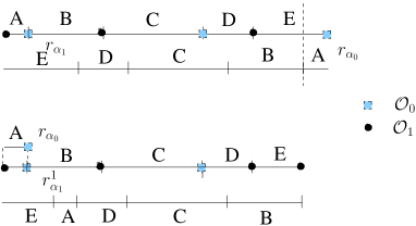
(a) Case $\lambda_{\alpha_{0}}>\lambda_{\alpha_{1}}$ or $\epsilon(\lambda,\pi)=0$.

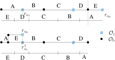
(b) Case $\lambda_{\alpha_{0}}<\lambda_{\alpha_{1}}$ or $\epsilon(\lambda,\pi)=1$.

Figure 1. Rauzy Veech induction

The IET $\widetilde{T}$ fulfills the Keane condition as well. Therefore we can iterate the renormalization procedure and generate a sequence of IETs $(\mathcal{R}^{n}(T))_{n\geq 0}$. Denote by $\pi^{n}=(\pi^{n}_{0},\pi^{n}_{1})\in\mathcal{S}^{0}_{\mathcal{A}}$ and $\lambda^{n}=(\lambda^{n}_{\alpha})_{\alpha\in\mathcal{A}}$ respectively the pair and the vector which determine $\mathcal{R}^{n}(T)$. Then $\mathcal{R}^{n}(T)$ is the first return map of $T$ to the interval $I^{n}=[0,|\lambda^{n}|)$ and

$$\lambda=\Theta^{(n)}(T)\lambda^{n}\text{ with }\Theta^{(n)}(T)=\Theta(T)\cdot\Theta(\mathcal{R}(T))\cdot\ldots\cdot\Theta(\mathcal{R}^{n-1}(T)).$$

We denote by $I^{n}_{\alpha}=[l^{n}_{\alpha},r^{n}_{\alpha})$ the intervals exchanged by $\mathcal{R}^{n}(T)$.

Let $T:I\to I$ be an arbitrary IET satisfying the Keane condition. Suppose that $(n_{k})_{k\geq 0}$ is an increasing sequence of natural numbers such $n_{0}=0$ and set

(2.8) $$Z(k+1):=\Theta(\mathcal{R}^{n_{k}}(T))\cdot\Theta(\mathcal{R}^{n_{k}+1}(T))\cdot\ldots\cdot\Theta(\mathcal{R}^{n_{k+1}-1}(T))$$

Since $\lambda^{n_{k}}=Z(k+1)\lambda^{n_{k+1}}$, if for each $k<k^{\prime}$ we let

(2.9) $$Q(k,k^{\prime})=Z(k+1)\cdot Z(k+2)\cdot\ldots\cdot Z(k^{\prime})$$

then we have $\lambda^{n_{k}}=Q(k,k^{\prime})\lambda^{n_{k^{\prime}}}$. We will write $Q(k)$ for $Q(0,k)$. By definition, $\mathcal{R}^{n_{k^{\prime}}}(T):I^{n_{k^{\prime}}}\to I^{n_{k^{\prime}}}$ is the first return map of $\mathcal{R}^{n_{k}}(T):I^{n_{k}}\to I^{n_{k}}$ to the interval $I^{n_{k}}\subset I^{n_{k^{\prime}}}$. Moreover, $Q_{\alpha\beta}(k,k^{\prime})$ is the time spent by any point of $I^{n_{k^{\prime}}}_{\beta}$ in $I^{n_{k}}_{\alpha}$ until it returns to $I^{n_{k^{\prime}}}$. It follows that

$$Q_{\beta}(k,k^{\prime})=\sum_{\alpha\in\mathcal{A}}Q_{\alpha\beta}(k,k^{\prime})$$

is the first return time of points of $I^{n_{k^{\prime}}}_{\beta}$ to $I^{n_{k^{\prime}}}$.

In what follows, the norm of a vector is defined as the largest absolute value of the coefficients and for any matrix $B=[B_{\alpha\beta}]_{\alpha,\beta\in\mathcal{A}}$ we set $\|B\|=\max_{\beta\in\mathcal{A}}\sum_{\alpha\in\mathcal{A}}|B_{\alpha\beta}|$.

IETs of periodic type

Definition 3 (see [41]).

An IET $T$ is of periodic type if there exists $p>0$ (called a period of $T$) such that $\Theta(\mathcal{R}^{n+p}(T))=\Theta(\mathcal{R}^{n}(T))$ for every $n\geq 0$ and $A=A(T):=\Theta^{(p)}(T)$ (called a period matrix of $T$) has strictly positive entries.

Since the set $\mathcal{S}^{0}_{\mathcal{A}}$ is finite, up to taking a multiple of the period $p$ if necessary, we can assume that $\pi^{p}=\pi$. We will always assume that the period $p$ is chosen so that $\pi^{p}=\pi$. Explicit examples of IETs of periodic type appear in [41]. The procedure to construct them is based on choosing closed paths on Rauzy class and using the following Remark.

Remark 2.4.

Suppose that $T=T_{(\pi,\lambda)}$ is of periodic type with period matrix $A=\Theta^{(p)}(T)$. It follows that $\lambda=A^{n}\lambda^{pn}\in A^{n}{\mathbb{R}}^{\mathcal{A}}_{+}$ and hence $\lambda$ belongs to $\bigcap_{n\geq 0}A^{n}{\mathbb{R}}^{\mathcal{A}}_{+}$ which is a one-dimensional convex cone (see [48]). Therefore $\lambda$ is a positive right Perron-Frobenius eigenvector of the matrix $\Theta^{(p)}(T)$. It follows that $(\pi^{p},\lambda^{p}/|\lambda^{p}|)=(\pi,\lambda/|\lambda|)$ and $|\lambda|/|\lambda^{p}|$ is the Perron-Frobenius eigenvector of the matrix $A$.

Remark 2.5.

IETs of periodic type automatically satisfy the Keane condition. Indeed, $T$ satisfies the Keane condition if and only if the orbit of $T$ under $\mathcal{R}$ is infinite (see [31]) and IETs of periodic type by definition have an infinite (periodic) orbit under $\mathcal{R}$. Moreover, using the methods in [47] (see also [51]) one can show that every IET of periodic type is uniquely ergodic.

Suppose that $T=T_{(\pi,\lambda)}$ is of periodic type and let $A=\Theta^{(p)}(T)$. By (2.7),

$$A^{t}\Omega_{\pi}A=\Omega_{{\pi}}\text{ and hence }\ker\Omega_{{\pi}}=A\ker\Omega_{{\pi}}\text{ and }H_{{\pi}}=A^{t}H_{{\pi}}.$$

Moreover, multiplying the period $p$ if necessary, we can assume that $A|_{\ker\Omega_{\pi}}=Id$ (see Remark 2.11 for details). Denote by $Sp(A)$ the set of complex eigenvalues of $A$, including multiplicities. Let us consider the set of Lyapunov exponents $\{\log|\rho|:\rho\in Sp(A)\}$. It consists of the numbers

$$\theta_{1}>\theta_{2}\geq\theta_{3}\geq\ldots\geq\theta_{g}\geq 0=\ldots=0\geq-\theta_{g}\geq\ldots\geq-\theta_{3}\geq-\theta_{2}>-\theta_{1},$$

where $2g=\dim H_{\pi}$ and $0$ occurs with the multiplicity $\kappa-1=\dim\ker\Omega_{{\pi}}$ (see e.g. [54]). Moreover, $\rho_{1}:=\exp\theta_{1}$ is the Perron-Frobenius eigenvalue of $A$.

Definition 4.

An IET $T_{(\pi,\lambda)}$ is of hyperbolic periodic type if it is of periodic type and $A^{t}:H_{\pi}\to H_{\pi}$ is a hyperbolic linear map, or equivalently $\theta_{g}>0$.

Convention.

When $T$ is of periodic type, we will always consider iterates of $\mathcal{R}$ corresponding to the sequence $(pk)_{k\geq 0}$, where $p$ is a period of $T$ and $A$ the associated periodic matrix, chosen so that $\pi^{p}=\pi$ and $A|_{\ker\Omega_{\pi}}=Id$.

Definition 5.

Suppose that $T=T_{(\pi,\lambda)}$ is of periodic type with period $p$ and period matrix $A=\Theta^{(p)}(T)$ as above. In this case we will denote by $T^{(k)}=(\pi^{(k)},\lambda^{(k)})$ the IET $\mathcal{R}^{pk}(T)$, by $I^{(k)}=[0,|\lambda^{kp}|)$ the interval on which $T^{(k)}$ is defined and by $I_{\alpha}^{(k)}=[l_{\alpha}^{(k)},r_{\alpha}^{(k)})$ the intervals exchanged by $T^{(k)}$.

Convention.

In the rest of the paper, when $T$ is of periodic type, the matrices $Z(k)$ and $Q(k)$ will denote be the matrices associated to the sequence $(pk)_{k\geq 0}$ by (2.8) and (2.9) respectively. Clearly $Z(k)=A$ and $Q(k,k^{\prime})=A^{k^{\prime}-k}=Q(k^{\prime}-k)$ for all $0\leq k\leq k^{\prime}$.

In the spirit of [49], we set $\nu_{1}(A)=\max\{{A_{\alpha\gamma}}/{A_{\beta\gamma}}:\alpha,\beta,\gamma\in\mathcal{A}\}$, $\nu_{2}(A)=\nu_{1}(A^{T})=\max\{{A_{\gamma\alpha}}/{A_{\gamma\beta}}:\alpha,\beta,\gamma\in\mathcal{A}\}$ and let $\nu(A)=\max\{\nu_{1}(A),\nu_{2}(A)\}$. Since $\lambda^{(k)}=A\lambda^{(k+1)}$ and for any $k\geq 1$ we have $Q(k)=Q(k-1)A$, we have

(2.10) $$\frac{|I^{(k)}_{\beta}|}{\nu(A)}\leq|I^{(k)}_{\alpha}|\leq\nu(A)|I^{(k)}_{\beta}|,\quad\frac{Q_{\beta}(k)}{\nu(A)}\leq Q_{\alpha}(k)\leq\nu(A)Q_{\beta}(k)\quad\forall\alpha,\beta\in\mathcal{A}.$$

From the above relation, it also follows that Rohlin towers have comparable areas, that is, since by Rohlin’s Lemma and Pigeon Hole principle there exists $\beta$ such that $Q_{\beta}(k)|I^{(k)}_{\beta}|\geq|I|/d$, one has

(2.11) $$\frac{1}{d\nu(A)^{2}|I^{(0)}|}\leq Q_{\alpha}(k)|I^{(k)}_{\alpha}|\leq|I^{(0)}|,\quad\text{ for all }\alpha\in\mathcal{A}.$$

A bases for the kernel

Let $p:\{0,1,\ldots,d,d+1\}\to\{0,1,\ldots,d,d+1\}$ stand for the permutation

$$p(j)=\left\{\begin{matrix}\pi_{1}\circ\pi^{-1}_{0}(j)&\text{ if }&1\leq j\leq d\\ j&\text{ if }&j=0,d+1.\end{matrix}\right.$$

Following [48, 49], denote by $\sigma=\sigma_{\pi}$ the corresponding permutation on $\{0,1,\ldots,d\}$,

$$\sigma(j)=p^{-1}(p(j)+1)-1\text{ for }0\leq j\leq d.$$

Then $\widehat{T}_{(\pi,\lambda)}r_{\pi_{0}^{-1}(j)}={T}_{(\pi,\lambda)}r_{\pi_{0}^{-1}(\sigma j)}$ for all $j\neq 0,p^{-1}(d)$. Denote by $\Sigma(\pi)$ the set of orbits for the permutation $\sigma$. Let $\Sigma_{0}(\pi)$ stand for the subset of orbits that do not contain zero.

Remark 2.6.

If $T$ is obtained from a minimal flow $(\phi_{t})_{t\in{\mathbb{R}}}$ on a surface $S$ as Poincaré first return map to a transversal, then the orbits $\mathcal{O}\in\Sigma(\pi)$ are in one to one correspondence with saddle points of $(\phi_{t})_{t\in{\mathbb{R}}}$. Hence $\#\Sigma(\pi)=\kappa$, where $\kappa$ is the number of saddle points of $(\phi_{t})_{t\in{\mathbb{R}}}$.

For every $\mathcal{O}\in\Sigma(\pi)$ denote by $b(\mathcal{O})\in{\mathbb{R}}^{\mathcal{A}}$ the vector given by

(2.12) $$b(\mathcal{O})_{\alpha}=\chi_{\mathcal{O}}(\pi_{0}(\alpha))-\chi_{\mathcal{O}}(\pi_{0}(\alpha)-1)\text{ for }\alpha\in\mathcal{A},$$

where $\chi_{\mathcal{O}}(j)=1$ iff $j\in\mathscr{O}$ and $0$ otherwise. Moreover, for every $\mathcal{O}\in\Sigma(\pi)$, we denote by

(2.13) $$\mathcal{A}^{-}_{\mathcal{O}}=\{\alpha\in\mathcal{A},\ \pi_{0}(\alpha)\in\mathcal{O}\},\qquad\mathcal{A}^{+}_{\mathcal{O}}=\{\alpha\in\mathcal{A},\ \pi_{0}(\alpha)-1\in\mathcal{O}\}.$$

If $\alpha\in\mathcal{A}_{\mathcal{O}}^{+}$ (respectively $\alpha\in\mathcal{A}_{\mathcal{O}}^{-}$ ) then the left (respectively right) endpoint of $I_{\alpha}$ belongs to a separatrix of the saddle represented by $\mathcal{O}$.

Lemma 2.7 (see [49]).

For every irreducible pair $\pi$ we have $\sum_{\mathcal{O}\in\Sigma(\pi)}b(\mathcal{O})=0$, the vectors $b(\mathcal{O})$, $\mathcal{O}\in\Sigma_{0}(\pi)$ are linearly independent and the linear subspace generated by them is equal to $\ker\Omega_{\pi}$. Moreover, $h\in H_{\pi}$ if and only if $\langle h,b(\mathcal{O)}\rangle=0$ for every $\mathcal{O}\in\Sigma(\pi)$. $\Box$

Remark 2.8.

Let $\Lambda^{\pi}:{\mathbb{R}}^{\mathcal{A}}\to{\mathbb{R}}^{\Sigma_{0}(\pi)}$ stand for the linear transformation given by $(\Lambda^{\pi}h)_{\mathcal{O}}=\langle h,b(\mathcal{O)}\rangle$ for $\mathcal{O}\in\Sigma_{0}(\pi)$. By Lemma 2.7, $H_{\pi}=\ker\Lambda^{\pi}$ and if ${\mathbb{R}}^{\mathcal{A}}=F\oplus H_{\pi}$ is a direct sum decomposition then $\Lambda^{\pi}:F\to{\mathbb{R}}^{\Sigma_{0}(\pi)}$ establishes an isomorphism of linear spaces. It follows that there exists $K_{F}>0$ such that

$$\|h\|\leq K_{F}\|\Lambda^{\pi}h\|\;\;\text{ for all }\;\;h\in F.$$

Lemma 2.9 (see [49]).

Suppose that $T_{(\widetilde{\pi},\widetilde{\lambda})}=\mathcal{R}(T_{(\pi,\lambda)})$. Then there exists a bijection $\xi:\Sigma(\pi)\to\Sigma(\widetilde{\pi})$ that depends only on $(\pi,\lambda)$ such that $\Theta(\pi,\lambda)^{-1}b(\mathcal{O})=b(\xi\mathcal{O})$ for $\mathcal{O}\in\Sigma(\pi)$.$\Box$

Moreover, analyzing the explicit correspondence given by $\xi$ (we refer the reader for example to the formulas in [51], §2.4) one can check that we have the following. For $\upsilon=0,1$, let $\alpha_{\upsilon}\in\mathcal{A}$ be such that $\pi_{\upsilon}(\alpha_{\upsilon})=d$. Define the orbits $\mathcal{O}_{0},\mathcal{O}_{1}\in\Sigma(\pi)$ (where possibly $\mathcal{O}_{0}=\mathcal{O}_{1}$) as follows. Let $\varepsilon=\varepsilon(\pi,\lambda)$ is as in (2.5) and Let $\mathcal{O}_{\varepsilon}\in\Sigma(\pi)$ such that $d\in\mathcal{O}_{\varepsilon}$. Remark that $\alpha_{0},\alpha_{1}\in\mathcal{A}_{\mathcal{O}_{\varepsilon}}^{-}$ since $\pi_{0}(\alpha_{0})=\pi_{1}(\alpha_{1})=d\in\mathcal{O}_{\varepsilon}$. Let $\mathcal{O}_{1-\varepsilon}$ be such that $\alpha_{1-\varepsilon}\in\mathcal{A}_{\mathcal{O}_{1-\varepsilon}}^{+}$. Denote by $\widetilde{\mathcal{A}}^{\pm}_{\mathcal{O}}$, $\mathcal{O}\in\Sigma(\widetilde{\pi})$ the corresponding sets for the pair $\widetilde{\pi}$.

Lemma 2.10.

For each $\mathcal{O}\in\Sigma(\pi)$, $\widetilde{\mathcal{A}}^{+}_{\xi\mathcal{O}_{\varepsilon}}=\mathcal{A}^{+}_{\mathcal{O}_{\varepsilon}}$. For each $\mathcal{O}\notin\{\mathcal{O}_{0},\mathcal{O}_{1}\}$ or if $\mathcal{O}=\mathcal{O}_{0}=\mathcal{O}_{1}$, then $\widetilde{\mathcal{A}}^{-}_{\xi\mathcal{O}}=\mathcal{A}^{-}_{\mathcal{O}}$. If $\mathcal{O}_{0}\neq\mathcal{O}_{1}$, then $\widetilde{\mathcal{A}}^{-}_{\xi\mathcal{O}_{\varepsilon}}=\mathcal{A}^{-}_{\mathcal{O}_{\varepsilon}}\backslash\{\alpha_{\varepsilon}\}$ and $\widetilde{\mathcal{A}}^{-}_{\xi\mathcal{O}_{1-\varepsilon}}=\mathcal{A}^{-}_{\mathcal{O}_{1-\varepsilon}}\cup\{\alpha_{\varepsilon}\}$.

An example of these correspondence of orbits is illustrated in Figure 1.

Remark 2.11.

If $T$ is of periodic type, let us remark that $\Sigma(\pi^{(k)})=\Sigma(\pi^{(k^{\prime})})=\Sigma(\pi)$ for every $k^{\prime}\geq k\geq 0$. Up to replacing the period $p$ by a multiple, we can assume that $Q(k,k^{\prime})b(\mathcal{O})=b(\mathcal{O})$ for each $\mathcal{O}\in\Sigma(\pi^{(k)})$ and $0\leq k\leq k^{\prime}$.

2.3. Cocycles with logarithmic singularities

Denote by $\operatorname{BV}(\sqcup_{\alpha\in\mathcal{A}}I^{(k)}_{\alpha})$ the space of functions $\varphi:I^{(k)}\to\mathbb{R}$ such that the restriction $\varphi:I^{(k)}_{\alpha}\to\mathbb{R}$ is of bounded variation for every $\alpha\in\mathcal{A}$. Let us denote by ${\operatorname{Var}}\!\left.\!\left({f}\right)\right|_{J}$ the total variation of ${f}$ on the interval $J\subset I$. Then set

(2.14) $$\operatorname{Var}\varphi=\sum_{\alpha\in\mathcal{A}}{\operatorname{Var}}\!\left.\!\left(\varphi\right)\right|_{I^{(k)}_{\alpha}}.$$

The space $\operatorname{BV}(\sqcup_{\alpha\in\mathcal{A}}I^{(k)}_{\alpha})$ is equipped with the norm $\|\varphi\|_{\operatorname{BV}}=\|\varphi\|_{\sup}+\operatorname{Var}\varphi$. Denote by $\operatorname{BV}_{0}(\sqcup_{\alpha\in\mathcal{A}}I^{(k)}_{\alpha})$ the subspace of all functions in $\operatorname{BV}(\sqcup_{\alpha\in\mathcal{A}}I^{(k)}_{\alpha})$ with zero mean.

For every function $\varphi\in\operatorname{BV}(\sqcup_{\alpha\in\mathcal{A}}I_{\alpha})$ and $x\in I$ we will denote by $\varphi_{+}(x)$ and $\varphi_{-}(x)$ the right-handed and left-handed limit of $\varphi$ at $x$ respectively. Denote by $\operatorname{AC}(\sqcup_{\alpha\in\mathcal{A}}I_{\alpha})$ the space of functions $\varphi:I\to\mathbb{R}$ which are absolutely continuous on the interior of each $I_{\alpha}$, $\alpha\in\mathcal{A}$ and by $\operatorname{AC}_{0}(\sqcup_{\alpha\in\mathcal{A}}I_{\alpha})$ its subspace of zero mean functions. For any $\varphi\in\operatorname{AC}(\sqcup_{\alpha\in\mathcal{A}}I_{\alpha})$ let

$$s(\varphi)=\int_{I}\varphi^{\prime}(x)\,dx=\sum_{\alpha\in\mathcal{A}}(\varphi_{-}(r_{\alpha})-\varphi_{+}(l_{\alpha})).$$

Denote by $\operatorname{BV}^{1}(\sqcup_{\alpha\in\mathcal{A}}I_{\alpha})$ the space of functions $\varphi\in\operatorname{AC}(\sqcup_{\alpha\in\mathcal{A}}I_{\alpha})$ such that $\varphi^{\prime}\in\operatorname{BV}(\sqcup_{\alpha\in\mathcal{A}}I_{\alpha})$ and by $\operatorname{BV}_{*}^{1}(\sqcup_{\alpha\in\mathcal{A}}I_{\alpha})$ its subspace of functions $\varphi$ for which $s(\varphi)=0$.

Theorem 2.12 (see [31] and [32]).

If $T:I\to I$ satisfies a Roth type condition then each cocycle $\varphi\in\operatorname{BV}_{*}^{1}(\sqcup_{\alpha\in\mathcal{A}}I_{\alpha})$ for $T$ is cohomologous (via a continuous transfer function) to a cocycle which is constant on each interval $I_{\alpha}$, $\alpha\in\mathcal{A}$. Moreover, the set of IETs satisfying this Roth type condition has full measure and contains all IETs of periodic type.

The prove of the above result is based on the following conclusion from the Gottschalk-Hedlund theorem (see §3.4 in [32]).

Proposition 2.13.

If $T$ satisfies the Keane condition and $\varphi\in\operatorname{AC}_{0}(\sqcup_{\alpha\in\mathcal{A}}I_{\alpha})$ is a function such that the sequence $(\varphi^{(n)})_{n\geq 0}$ is uniformly bounded then $\varphi$ is a coboundary with a continuous transfer function.

Denote by $\operatorname{PL}(\sqcup_{\alpha\in\mathcal{A}}I_{\alpha})$ the set of functions $\varphi:I\to{\mathbb{R}}$ such that $\varphi(x)=sx+c_{\alpha}$ for $x\in I_{\alpha}$. As a consequence of Theorem 2.12 we have the following.

Corollary 2.14.

If the IET $T:I\to I$ is of periodic type then each cocycle $\varphi\in\operatorname{BV}^{1}(\sqcup_{\alpha\in\mathcal{A}}I_{\alpha})$ is cohomologous (via a continuous transfer function) to a cocycle $\varphi_{pl}\in\operatorname{PL}(\sqcup_{\alpha\in\mathcal{A}}I_{\alpha})$ with $s({\varphi}_{pl})=s(\varphi)$.

In the Introduction §1 we defined the space $\operatorname{LG}(\sqcup_{\alpha\in\mathcal{A}}I_{\alpha})$ of functions with logarithmic singularities of geometric type (see Definition 1) and the subspace $\operatorname{LSG}(\sqcup_{\alpha\in\mathcal{A}}I_{\alpha})$ of symmetric logarithmic singularities of geometric type, which satisfy the symmetry condition (1.3). We denote by $\operatorname{LG}_{0}(\sqcup_{\alpha\in\mathcal{A}}I_{\alpha})$ and $\operatorname{LSG}_{0}(\sqcup_{\alpha\in\mathcal{A}}I_{\alpha})$ the corresponding spaces of functions with zero mean.

Definition 6.

A function $\varphi\in\operatorname{LG}(\sqcup_{\alpha\in\mathcal{A}}I_{\alpha})$ of the form (1.2) has strong symmetric logarithmic singularities if for every $\mathcal{O}\in\Sigma(\pi)$ we have

(2.15) $$\sum_{\alpha\in\mathcal{A}_{\mathcal{O}}^{-}}C^{-}_{\alpha}-\sum_{\alpha\in\mathcal{A}_{\mathcal{O}}^{+}}C^{+}_{\alpha}=0,$$

where $\mathcal{A}_{\mathcal{O}}^{-},\mathcal{A}_{\mathcal{O}}^{+}$ are the sets defined in (2.13).

Denote by $\operatorname{LSSG}(\sqcup_{\alpha\in\mathcal{A}}I_{\alpha})$ the space of functions with strong symmetric logarithmic singularities of geometric type and let $\operatorname{LSSG}_{0}:=\operatorname{LSSG}\cap\operatorname{LG}_{0}$. Clearly $\operatorname{LSSG}(\sqcup_{\alpha\in\mathcal{A}}I_{\alpha})\subset\operatorname{LSG}(\sqcup_{\alpha\in\mathcal{A}}I_{\alpha})$ since the condition (2.15) implies the weaker symmetry condition (1.3) by summing over $\mathcal{O}\in\Sigma$. Strong symmetric singularities of geometric type appear naturally from extensions of locally Hamiltonian flows, see §6. This stronger condition of symmetry is important in the proof of ergodicity.

We will also use the space $\overline{\operatorname{LG}}(\sqcup_{\alpha\in\mathcal{A}}I_{\alpha})={\operatorname{LG}}(\sqcup_{\alpha\in\mathcal{A}}I_{\alpha})+{\operatorname{BV}}(\sqcup_{\alpha\in\mathcal{A}}I_{\alpha})$ (respectively $\overline{\operatorname{LSSG}}(\sqcup_{\alpha\in\mathcal{A}}I_{\alpha})={\operatorname{LSSG}}(\sqcup_{\alpha\in\mathcal{A}}I_{\alpha})+{\operatorname{BV}}(\sqcup_{\alpha\in\mathcal{A}}I_{\alpha})$), i.e. the space of all functions with logarithmic singularities (respectively strong symmetric logarithmic singularities) of geometric type and zero mean of the form (1.2) for which we require only that $g_{\varphi}\in\operatorname{BV}(\sqcup_{\alpha\in\mathcal{A}}I_{\alpha})$. We will denote by $\overline{\operatorname{LG}}_{0}$ and $\overline{\operatorname{LSSG}}_{0}$ their subspaces of zero mean functions.

Note that the space $\operatorname{BV}$ $(\operatorname{BV}^{1})$ coincides with the subspace of functions $\varphi\in\overline{\operatorname{LG}}$ ($\operatorname{LG}$) as in (1.2) such that $C^{\pm}_{\alpha}=0$ for all $\alpha\in\mathcal{A}$.

Definition 7.

For every $\varphi\in\overline{\operatorname{LG}}(\sqcup_{\alpha\in\mathcal{A}}I_{\alpha})$ of the form (1.2) set

$$\mathscr{L}(\varphi)=\sum_{\alpha\in\mathcal{A}}(|C^{+}_{\alpha}|+|C^{-}_{\alpha}|)\quad\text{ and }\quad\mathscr{LV}(\varphi):=\mathscr{L}(\varphi)+\operatorname{Var}g_{\varphi}.$$

The quantity $\mathscr{LV}(\varphi)$ will play throughout the paper an essential role to bound functions $\overline{\operatorname{LG}}$, since it controls simultaneously the logarithmic singularities, through the logarithmic constants $\mathscr{L}(\varphi)$, and the part of bounded variation.

The spaces $\overline{\operatorname{LSSG}}(\sqcup_{\alpha\in\mathcal{A}}I_{\alpha})$ and $\overline{\operatorname{LSSG}}_{0}(\sqcup_{\alpha\in\mathcal{A}}I_{\alpha})$ equipped with the norm

$$\|\varphi\|_{\mathscr{LV}}=\mathscr{L}(\varphi)+\|g_{\varphi}\|_{\operatorname{BV}}$$

become Banach spaces for which ${\operatorname{LSSG}}(\sqcup_{\alpha\in\mathcal{A}}I_{\alpha})$ or respectively $\operatorname{LSSG}_{0}(\sqcup_{\alpha\in\mathcal{A}}I_{\alpha})$ are dense subspaces.

For every integrable function $f:I\to{\mathbb{R}}$ and a subinterval $J\subset I$ let $m(f,J)$ stand for the mean value of $f$ on $J$, this is

$$m(f,J)=\frac{1}{|J|}\int_{J}f(x)\,dx.$$

Proposition 2.15.

If $\varphi\in\overline{\operatorname{LG}}(\sqcup_{\alpha\in\mathcal{A}}I_{\alpha})$ and $J\subset I_{\alpha}$ for some $\alpha\in\mathcal{A}$ then

(2.16) $$|m(\varphi,J)-m(\varphi,I_{\alpha})|\leq\mathscr{LV}(\varphi)\left(4+\frac{|I_{\alpha}|}{|J|}\right)$$

and

(2.17) $$\frac{1}{|J|}\int_{J}|\varphi(x)-m(\varphi,J)|\,dx\leq 8\mathscr{LV}(\varphi).$$

The proof of Proposition 2.15 is elementary, but we include the proof for completeness in Appendix A.

Definition 8.

For every $\varphi\in\overline{\operatorname{LSSG}}(\sqcup_{\alpha\in\mathcal{A}}I_{\alpha})$ and $\mathcal{O}\in\Sigma(\pi)$ set

$$\mathcal{O}(\varphi)=\lim_{x\to 0^{+}}\left(\sum_{\alpha\in\mathcal{A},\pi_{0}(\alpha)\in\mathcal{O}}\varphi(r_{\alpha}-x)-\sum_{\alpha\in\mathcal{A},\pi_{0}(\alpha)-1\in\mathcal{O}}\varphi(l_{\alpha}+x)\right).$$

In order to prove that $\mathcal{O}(\varphi)$ is finite, we need the strong symmetry condition (2.15).

Lemma 2.16.

For every $\varphi\in\overline{\operatorname{LSSG}}(\sqcup_{\alpha\in\mathcal{A}}I_{\alpha})$ and $\mathcal{O}\in\Sigma(\pi)$, $\mathcal{O}(\varphi)$ is finite. Moreover, if $\varphi\in\operatorname{LSSG}(\sqcup_{\alpha\in\mathcal{A}}I_{\alpha})$ then

$$|\mathcal{O}(\varphi)|\leq 2d\nu(A)\frac{1}{|I|}\int_{I}|\varphi(x)|\,dx+2d\mathscr{LV}(\varphi).$$

Proof.

Let $a:=\min\{|I_{\alpha}|:\alpha\in\mathcal{A}\}/2$. Then for $x\in(0,a)$ we have

$$\varphi(r_{\alpha}-x)=-C_{\alpha}^{-}\log(x)+g^{-}_{\alpha}(x)\text{ and }\varphi(l_{\alpha}+x)=-C_{\alpha}^{+}\log(x)+g^{+}_{\alpha}(x),$$

where $g^{\pm}_{\alpha}:[0,a]\to{\mathbb{R}}$ is of bounded variation for $\alpha\in\mathcal{A}$. Therefore, using the symmetry condition (2.15)

$$\begin{split}\Delta(x):=&\sum_{\alpha\in\mathcal{A}_{\mathcal{O}^{-}}}\varphi(r_{\alpha}-x)-\sum_{\alpha\in\mathcal{A}_{\mathcal{O}}^{+}}\varphi(l_{\alpha}+x)=-\sum_{\alpha\in\mathcal{A}_{\mathcal{O}}^{-}}C^{-}_{\alpha}\log(x)+\sum_{\alpha\in\mathcal{A}_{\mathcal{O}}^{-}}g^{-}_{\alpha}(x)\\ &+\sum_{\alpha\in\mathcal{A}_{\mathcal{O}}^{+}}C^{+}_{\alpha}\log(x)-\sum_{\alpha\in\mathcal{A}_{\mathcal{O}}^{+}}g^{+}_{\alpha}(x)=\sum_{\alpha\in\mathcal{A}_{\mathcal{O}}^{-}}g^{-}_{\alpha}(x)-\sum_{\alpha\in\mathcal{A}_{\mathcal{O}}^{+}}g^{+}_{\alpha}(x).\end{split}$$

It follows that $\mathcal{O}(\varphi)$ is finite and given by

(2.18) $$\mathcal{O}(\varphi)=\Delta_{+}(0)=\sum_{\alpha\in\mathcal{A}_{\mathcal{O}}^{-}}(g^{-}_{\alpha})_{+}(0)-\sum_{\alpha\in\mathcal{A}_{\mathcal{O}}^{+}}(g^{+}_{\alpha})_{+}(0).$$

Suppose now that $\varphi\in\operatorname{LSSG}(\sqcup_{\alpha\in\mathcal{A}}I_{\alpha})$ is of the form (1.2). Then $g^{\pm}_{\alpha}$ are absolutely continuous and $|(g^{+}_{\alpha})^{\prime}(x)|\leq\mathscr{L}(\varphi)/a+|g_{\varphi}^{\prime}(l_{\alpha}+x)|$ and $|(g^{-}_{\alpha})^{\prime}(x)|\leq\mathscr{L}(\varphi)/a+|g_{\varphi}^{\prime}(r_{\alpha}-x)|$, and hence

$$|\Delta^{\prime}(x)|\leq\frac{2d\mathscr{L}(\varphi)}{a}+\sum_{\alpha\in\mathcal{A}}(|g_{\varphi}^{\prime}(l_{\alpha}+x)|+|g_{\varphi}^{\prime}(r_{\alpha}-x)|)\text{ for }x\in[0,a].$$

Therefore, for $x,y\in[0,a]$,

(2.19) $$\begin{split}|\Delta(x)-\Delta(y)|&\leq 2d\mathscr{L}(\varphi)+\sum_{\alpha\in\mathcal{A}}(\int_{x}^{y}|g_{\varphi}^{\prime}(l_{\alpha}+t)|dt+\int_{x}^{y}|g_{\varphi}^{\prime}(r_{\alpha}-t)|dt)\\ &\leq 2d\mathscr{L}(\varphi)+\sum_{\alpha\in\mathcal{A}}(\int_{l_{\alpha}}^{l_{\alpha}+a}|g_{\varphi}^{\prime}(t)|dt+\int_{r_{\alpha}-a}^{r_{\alpha}}|g_{\varphi}^{\prime}(t)|dt)\\ &\leq 2d\mathscr{L}(\varphi)+\int_{I}|g_{\varphi}^{\prime}(t)|dt=2d\mathscr{L}(\varphi)+\operatorname{Var}g_{\varphi}.\end{split}$$

Moreover, using the definition of $a$ and (2.10), one has

$$|m(\Delta,[0,a])| \leq\sum_{\alpha\in\mathcal{A},\pi_{0}(\alpha)\in\mathcal{O}}\left|m(\varphi,[r_{\alpha},r_{\alpha}-a])\right|+\sum_{\alpha\in\mathcal{A},\pi_{0}(\alpha)-1\in\mathcal{O}}\left|m(\varphi,[l_{\alpha},l_{\alpha}+a])\right|$$

$$\leq\frac{1}{a}\int_{I}|\varphi(x)|\,dx\leq 2d\nu(A)\frac{1}{|I|}\int_{I}|\varphi(x)|\,dx.$$

In view of the previous equation and (2.19), it follows that for all $x\in[0,a]$,

$$|\Delta(x)|\leq\sup_{y\in[0,a]}|\Delta(x)-\Delta(y)|+m(\Delta,[0,a])\leq\frac{2d\nu(A)}{|I|}\int_{I}|\varphi(x)|\,dx+2d\mathscr{L}(\varphi)+\operatorname{Var}g_{\varphi},$$

which completes the proof. ∎

Remark that if $\varphi\in\operatorname{BV}(\sqcup_{\alpha\in\mathcal{A}}I_{\alpha})$ and $\mathcal{O}\in\Sigma(\pi)$

(2.20) $$\mathcal{O}(\varphi)=\sum_{\alpha\in\mathcal{A},\pi_{0}(\alpha)\in\mathcal{O}}\varphi_{-}(r_{\alpha})-\sum_{\alpha\in\mathcal{A},\pi_{0}(\alpha)-1\in\mathcal{O}}\varphi_{+}(l_{\alpha}).$$

Hence, Definition 8 extends the definition of the operator $\mathcal{O}$ used by [7] for $\varphi\in\operatorname{BV}(\sqcup_{\alpha\in\mathcal{A}}I_{\alpha})$. Moreover, if $\varphi\in\operatorname{AC}(\sqcup_{\alpha\in\mathcal{A}}I_{\alpha})$ then

(2.21) $$\sum_{\mathcal{O}\in\Sigma(\pi)}\mathcal{O}(\varphi)=\sum_{\alpha\in\mathcal{A}}\varphi_{-}(r_{\alpha})-\sum_{\alpha\in\mathcal{A}}\varphi_{+}(l_{\alpha})=s(\varphi).$$

Remark 2.17.

If we identify the piecewise constant function $h(x)=\sum_{\alpha}h_{\alpha}\chi_{I_{\alpha}}(x)$ (where $\chi_{I_{\alpha}}$ is the characteristic function of $I_{\alpha}$) with the vector $h=(h_{\alpha})_{\alpha\in\mathcal{A}}$, note also that

$$\mathcal{O}(h)=\sum_{\pi_{0}(\alpha)\in\mathcal{O}}h_{\alpha}-\sum_{\pi_{0}(\alpha)-1\in\mathcal{O}}h_{\alpha}=\sum_{\alpha\in\mathcal{A}}(\chi_{\mathcal{O}}(\pi_{0}(\alpha))-\chi_{\mathcal{O}}(\pi_{0}(\alpha)-1))h_{\alpha}=\langle h,b(\mathcal{O})\rangle,$$

where $b(\mathcal{O})$, $\mathcal{O}\in\Sigma$ are the vectors defined in (2.12). In particular, Lemma 2.7 can be restated saying that the vector $h\in H_{\pi}$ if and only if for the corresponding function $h$ we have $\mathcal{O}(h)=0$ for every $\mathcal{O}\in\Sigma(\pi)$.

3. Renormalization of cocycles

Assume that $T$ is of periodic type and recall that we denote by $T^{(k)}=\mathcal{R}^{kp}(T)$ the sequence or Rauzy iterates corresponding to multiples of the period $p>0$.

Remark 3.1.

The definitions and Lemmas in §3.1 hold more in general for any IET satisfying the Keane condition and any subsequence $(T^{(k)})_{k\geq 0}$ which is of the form $(\mathcal{R}^{n_{k}}T)_{k\geq 0}$ for some subsequence $(n_{k})_{k\geq 0}$ of iterates of Rauzy-Veech induction.

3.1. Special Birkhoff sums

For every measurable cocycle $\varphi:I^{(k)}\to{\mathbb{R}}$ for the IET $T^{(k)}:I^{(k)}\to I^{(k)}$ and $k^{\prime}>k$ denote by $S(k,k^{\prime})\varphi:I^{(k^{\prime})}\to{\mathbb{R}}$ the renormalized cocycle for $T^{(k^{\prime})}$ given by

$$S(k,k^{\prime})\varphi(x)=\sum_{0\leq i<Q_{\beta}(k,k^{\prime})}\varphi((T^{(k)})^{i}x)\text{ for }x\in I^{(k^{\prime})}_{\beta}.$$

We write $S(k)\varphi$ for $S(0,k)\varphi$ and we adhere to the convention that $S(k,k)\varphi=\varphi$. Sums of this form are usually called special Birkhoff sums. If $\varphi$ is integrable then

(3.1) $$\|S(k,k^{\prime})\varphi\|_{L^{1}(I^{(k^{\prime})})}\leq\|\varphi\|_{L^{1}(I^{(k)})}\;\;\text{ and }$$

(3.2) $$\int_{I^{(k^{\prime})}}S(k,k^{\prime})\varphi(x)\,dx=\int_{I^{(k)}}\varphi(x)\,dx.$$

Note that the operator $S(k,k^{\prime})$ maps $\overline{\operatorname{LG}}(\sqcup_{\alpha\in\mathcal{A}}I^{(k)}_{\alpha})$ into $\overline{\operatorname{LG}}(\sqcup_{\alpha\in\mathcal{A}}I^{(k^{\prime})}_{\alpha})$. In view of (3.2), $S(k,k^{\prime})$ maps the space $\overline{\operatorname{LG}}_{0}(\sqcup_{\alpha\in\mathcal{A}}I^{(k)}_{\alpha})$ into $\overline{\operatorname{LG}}_{0}(\sqcup_{\alpha\in\mathcal{A}}I^{(k^{\prime})}_{\alpha})$. Moreover, we will show below (Lemma 3.3) that it also maps $\operatorname{LSSG}(\sqcup_{\alpha\in\mathcal{A}}I^{(k)}_{\alpha})$ into $\operatorname{LSSG}(\sqcup_{\alpha\in\mathcal{A}}I^{(k^{\prime})}_{\alpha})$. If $g\in\operatorname{BV}(\sqcup_{\alpha\in\mathcal{A}}I^{(k)}_{\alpha})$ then

(3.3) $$\operatorname{Var}S(k,k^{\prime})g\leq\operatorname{Var}g.$$

The following three Lemmas (Lemma 3.2, 3.3 and 3.4) allow us to compare the singularities of $S(k,k^{\prime})\varphi$ with the singularities of $\varphi$. Here the assumption that $\varphi$ is of geometric type plays a crucial role, since functions with symmetric singularities not of geometric type are not renormalized by the operation of considering special Birkhoff sums.

Lemma 3.2.

For each $k^{\prime}\geq k\geq 0$ and for each $\varphi\in\operatorname{LG}(\sqcup_{\alpha\in\mathcal{A}}I^{(k)}_{\alpha})$ of the form

$$\varphi(x)=-\sum_{\alpha\in\mathcal{A}}\left(C^{+}_{\alpha}\log\left(|I^{(k)}|\left\{\frac{x-l^{(k)}_{\alpha}}{|I^{(k)}|}\right\}\right)+C^{-}_{\alpha}\log\left(|I^{(k)}|\left\{\frac{r^{(k)}_{\alpha}-x}{|I^{(k)}|}\right\}\right)\right)$$

there exists a permutation $\chi:\mathcal{A}\rightarrow\mathcal{A}$ such that

$$S(k,k^{\prime})\varphi(x)= -\sum_{\alpha\in\mathcal{A}}C^{+}_{\alpha}\log(|I^{(k^{\prime})}|\{(x-l^{(k^{\prime})}_{\alpha})/|I^{(k^{\prime})}|\})$$

$$-\sum_{\alpha\in\mathcal{A}}C^{-}_{\chi(\alpha)}\log(|I^{(k^{\prime})}|\{(r^{(k^{\prime})}_{\alpha}-x)/|I^{(k^{\prime})}|\}+g(x),$$

where $g\in\operatorname{BV}^{1}(\sqcup_{\alpha\in\mathcal{A}}I^{(k^{\prime})}_{\alpha})$. In particular, $\mathscr{L}(S(k,k^{\prime})\varphi)=\mathscr{L}(\varphi)$.

Proof.

We will prove the Lemma for special Birkhoff sums corresponding to one single step of Rauzy induction. The proof then follows by induction on Rauzy steps. Let $\alpha_{0}:=\pi_{0}^{-1}(d)$ and $\alpha_{1}:=\pi_{1}^{-1}(d)$. Let write $C^{-}=(C^{-}_{\alpha})_{\alpha\in\mathcal{A}}$ for the vector in $\mathbb{R}^{\mathcal{A}}$ whose components are the constants $C_{\alpha}^{-}$. For $\upsilon=0,1$ let

$$G_{(\pi,\lambda)}^{\upsilon}=\{C^{-}=(C^{-}_{\alpha})_{\alpha\in\mathcal{A}}\in{\mathbb{R}}^{\mathcal{A}}:C^{-}_{\alpha_{\upsilon}}=0\}.$$

Let us consider $R:G_{(\pi,\lambda)}^{0}\cup G_{(\pi,\lambda)}^{1}\to G_{\mathcal{R}(\pi,\lambda)}^{\varepsilon(\pi,\lambda)}$ be given by

(3.4) $$R(C^{-})_{\alpha}=\left\{\begin{array}[]{ccc}C^{-}_{\alpha}&\text{ if }&\alpha\neq\alpha_{0},\alpha_{1},\\ C^{-}_{\alpha_{0}}+C^{-}_{\alpha_{1}}&\text{ if }&\alpha=\alpha_{1-\varepsilon(\pi,\lambda)},\\ 0&\text{ if }&\alpha=\alpha_{\varepsilon(\pi,\lambda)}.\end{array}\right.$$

Recall that for $(\pi^{1},\lambda^{1})=\mathcal{R}(\pi,\lambda)$ we have $\pi^{1}_{\varepsilon(\pi,\lambda)}(\alpha_{\varepsilon(\pi,\lambda)})=\pi_{\varepsilon(\pi,\lambda)}(\alpha_{\varepsilon(\pi,\lambda)})=d$, so $R(C^{-})\in G_{\mathcal{R}(\pi,\lambda)}^{\varepsilon(\pi,\lambda)}$. If $\varphi\in\operatorname{LG}(\sqcup_{\alpha\in\mathcal{A}}I_{\alpha})$ is of the form

$$\varphi(x)=-\sum_{\alpha\in\mathcal{A}}(C^{+}_{\alpha}\log(|I|\{(x-l_{\alpha})/|I|\})+C^{-}_{\alpha}\log(|I|\{(r_{\alpha}-x)/|I|\})),$$

then since the singularities are of geometric type, $C^{-}=(C^{-}_{\alpha})_{\alpha\in\mathcal{A}}\in G_{(\pi,\lambda)}^{\upsilon}$ for some $\upsilon=0,1$. Denote by $S^{1}\varphi$ the special Birkhoff sum corresponding to one step of Rauzy-Veech induction, given by

(3.5) $$S^{1}\varphi(x)=\sum_{0\leq i<\Theta(T)_{\beta}}\varphi(T^{i}(x)),\qquad\mathrm{for}\ x\in I^{1}_{\beta}.$$

Analyzing the effect of one step of Rauzy induction, one can then verify that

(3.6) $$S^{1}\varphi(x)= -\sum_{\alpha\in\mathcal{A}}\left(C^{+}_{\alpha}\log(|I^{1}|\{(x-l^{1}_{\alpha})/|I^{1}|\})\right.$$

$$+\left.R(C^{-})_{\alpha}\log(|I^{1}|\{(r^{1}_{\alpha}-x)/|I^{1}|\})\right)+g_{1}(x),$$

where $g_{1}\in\operatorname{BV}^{1}(\sqcup_{\alpha\in\mathcal{A}}I^{1}_{\alpha})$. See Figure 2. For $\upsilon=0,1$, define the permutation $\chi_{(\pi,\lambda)}^{\upsilon}:\mathcal{A}\to\mathcal{A}$ by

$$\chi_{(\pi,\lambda)}^{\upsilon}(\alpha_{\varepsilon(\pi,\alpha)})=\alpha_{\upsilon},\;\chi_{(\pi,\lambda)}^{\upsilon}(\alpha_{1-\varepsilon(\pi,\alpha)})=\alpha_{1-\upsilon},\;\chi_{(\pi,\lambda)}^{\upsilon}(\alpha)=\alpha\text{ for }\alpha\notin\{\alpha_{0},\alpha_{1}\}.$$

Remark then that since $\varphi\in G^{\upsilon}$, $\alpha_{\upsilon}\in\{\alpha_{0},\alpha_{1}\}$ is such that $C^{-}_{\alpha_{\upsilon}}=0$. Thus, one can verify that $R(C^{-})_{\alpha}=C^{-}_{\chi(\alpha)}$ for all $\alpha\in\mathcal{A}$. For $0\leq k<k^{\prime}$ and $\varphi\in G^{\upsilon}$, if we denote by $\varepsilon_{j}=\varepsilon(\pi^{j},\lambda^{j})$, we can let $\chi:=\chi^{\upsilon}(k,k^{\prime}):\mathcal{A}\to\mathcal{A}$ stand for the permutation

$$\chi:=\chi^{\upsilon}(k,k^{\prime})=\chi_{(\pi^{pk},\lambda^{pk})}^{\upsilon}\circ\chi_{(\pi^{pk+1},\lambda^{pk+1})}^{\varepsilon_{pk}}\circ\cdots\circ\chi_{(\pi^{pk^{\prime}-1},\lambda^{pk^{\prime}-1})}^{\varepsilon_{pk^{\prime}-2}}.$$

Then one can prove by induction on Rauzy steps that $R^{p(k^{\prime}-k)}(C^{-})_{\alpha}=C^{-}_{\chi(\alpha)}$. This together with $p(k^{\prime}-k)$ iterations of (3.6) concludes the proof. ∎

(a) Case $\lambda_{\alpha_{0}}>\lambda_{\alpha_{1}}$ or $\epsilon(\lambda,\pi)=0$.

(b) Case $\lambda_{\alpha_{0}}<\lambda_{\alpha_{1}}$ or $\epsilon(\lambda,\pi)=1$.

Figure 2. Renormalization of functions with logarithmic singularities of geometric type.

Consider the operator $\mathcal{O}(\varphi)$ defined in Definition 8.

Lemma 3.3.

For each $k^{\prime}\geq k\geq 0$ the operator $S(k,k^{\prime})$ maps $\overline{\operatorname{LSSG}}(\sqcup_{\alpha\in\mathcal{A}}I^{(k)}_{\alpha})$ into $\overline{\operatorname{LSSG}}(\sqcup_{\alpha\in\mathcal{A}}I^{(k^{\prime})}_{\alpha})$ and ${\operatorname{LSSG}}(\sqcup_{\alpha\in\mathcal{A}}I^{(k)}_{\alpha})$ into ${\operatorname{LSSG}}(\sqcup_{\alpha\in\mathcal{A}}I^{(k^{\prime})}_{\alpha})$. Moreover, for every $\varphi\in\operatorname{LSSG}(\sqcup_{\alpha\in\mathcal{A}}I^{(k)}_{\alpha})$ and $\mathcal{O}\in\Sigma(\pi)$, we have $\mathcal{O}(S(k,k^{\prime})\varphi)=\mathcal{O}(\varphi)$.

Proof.

Let $T=T_{\pi,\lambda}$, $\varphi\in\overline{\operatorname{LSSG}}(\sqcup_{\alpha\in\mathcal{A}}I_{\alpha})$ and consider the special Birkhoff sum $\widetilde{\varphi}=S^{1}\varphi$ given by one step of Rauzy-Veech induction (see (3.5)). Let $\xi$ be the correspondence between $\Sigma(\pi)$ and $\Sigma(\pi^{1})$ given by Lemma 2.9 and let $\mathcal{A}_{\mathcal{O}}^{\pm}$, $\mathcal{O}\in\Sigma(\pi)$, the sets defined in (2.13) and $\widetilde{\mathcal{A}}_{\mathcal{O}}^{\pm}$, $\mathcal{O}\in\Sigma(\pi^{1})$, the corresponding sets for $(\widetilde{\pi},\widetilde{\lambda})=(\pi^{1},\lambda^{1})$. We will show that

(3.7) $$\sum_{\alpha\in\mathcal{A}^{+}_{\mathcal{O}}}C^{+}_{\alpha} = \sum_{\alpha\in\widetilde{\mathcal{A}}^{+}_{\xi\mathcal{O}}}C^{+}_{\alpha}$$

(3.8) $$\sum_{\alpha\in\mathcal{A}^{-}_{\mathcal{O}}}C^{-}_{\alpha} = \sum_{\alpha\in\widetilde{\mathcal{A}}^{-}_{\xi\mathcal{O}}}R(C^{-})_{\alpha},$$

where $R$ is the operator defined in (3.4) in the proof of Lemma 3.2. Since by (3.6) the logarithmic constants for $S^{1}\varphi$ are the ones which appear in the right hand side, these two equations show that if the symmetry condition (2.15) holds for $\varphi$ for all $\mathcal{O}\in\Sigma(\pi)$, since $\xi:\Sigma(\pi)\to\Sigma(\pi^{1})$ is a bijection, the symmetry condition holds also for $S^{1}\varphi$ for all $\mathcal{O}\in\Sigma(\pi^{1})$. By induction on Rauzy steps, this shows that $S(k,k^{\prime})\varphi\in\overline{\operatorname{LSSG}}(\sqcup_{\alpha\in\mathcal{A}}I^{(k^{\prime})}_{\alpha})$ for each $k^{\prime}\geq k$. Let us prove (3.7, 3.8). Since $\widetilde{\mathcal{A}}^{+}_{\xi\mathcal{O}}={\mathcal{A}}^{+}_{\mathcal{O}}$ by Lemma 2.10, (3.7) holds trivially. From the definition (3.4) of $R$, one immediately sees that if $\mathcal{A}^{\prime}\subset\mathcal{A}$ is a subset such that either $\{\alpha_{0},\alpha_{1}\}\subset\mathcal{A^{\prime}}$ or $\{\alpha_{0},\alpha_{1}\}\cap\mathcal{A}^{\prime}=\emptyset$, then $\sum_{\alpha\in\mathcal{A}^{\prime}}C^{-}_{\alpha}-\sum_{\alpha\in\mathcal{A}^{\prime}}R(C^{-})_{\alpha}=0$. Since $\{\alpha_{0},\alpha_{1}\}\subset\mathcal{A}^{-}_{\mathcal{O}_{\epsilon}}$ (recall that $\pi_{0}(\alpha_{0})=\pi_{1}(\alpha_{1})=d\in\mathcal{O}_{\epsilon}$ by definition of $\mathcal{O}_{\epsilon}$) and thus $\{\alpha_{0},\alpha_{1}\}\cap\mathcal{A}^{-}_{\mathcal{O}}=\emptyset$ for all $\mathcal{O}\neq{\mathcal{O}_{\epsilon}}$, it follows that

$$\sum_{\alpha\in\mathcal{A}^{-}_{\mathcal{O}}}C^{-}_{\alpha}-\sum_{\alpha\in\mathcal{A}^{-}_{\mathcal{O}}}R(C^{-})_{\alpha}=0\quad\text{ for each }\quad\mathcal{O}\in\Sigma(\pi).$$

Thus, (3.8) holds also for $\mathcal{O}\in\{\mathcal{O}_{0},\mathcal{O}_{1}\}$ (where $\mathcal{O}_{0},\mathcal{O}_{1}$ were defined before Lemma 2.10) or if $\mathcal{O}=\mathcal{O}_{0}=\mathcal{O}_{1}$, since in these cases by Lemma 2.10 we can have $\mathcal{A}^{-}_{\mathcal{O}}=\widetilde{\mathcal{A}}^{-}_{\xi\mathcal{O}}$. Thus, we are left to consider the case in which $\mathcal{O}\notin\{\mathcal{O}_{0},\mathcal{O}_{1}\}$ and at the same time $\mathcal{O}_{0}\neq\mathcal{O}_{1}$. In these cases, since by Lemma 2.10 we have $\widetilde{\mathcal{A}}^{-}_{\xi\mathcal{O}_{\varepsilon}}=\mathcal{A}^{-}_{\mathcal{O}_{\varepsilon}}\backslash\{\alpha_{\varepsilon}\}$ and $\widetilde{\mathcal{A}}^{-}_{\xi\mathcal{O}_{1-\varepsilon}}=\mathcal{A}^{-}_{\mathcal{O}_{1-\varepsilon}}\cup\{\alpha_{\varepsilon}\}$, we can add or subtract $R(C^{-})_{\alpha_{\varepsilon}}$, which by (3.4) is equal to zero, to get respectively

$$\sum_{\alpha\in\mathcal{A}^{-}_{\mathcal{O}_{\varepsilon}}}C^{-}_{\alpha}-\sum_{\alpha\in\widetilde{\mathcal{A}}^{-}_{\xi\mathcal{O}_{\varepsilon}}}R(C^{-})_{\alpha}=\sum_{\alpha\in\mathcal{A}^{-}_{\mathcal{O}_{\varepsilon}}}(C^{-}_{\alpha}-R(C^{-})_{\alpha})+R(C^{-})_{\alpha_{\varepsilon}}=0,$$

$$\sum_{\alpha\in\mathcal{A}^{-}_{\mathcal{O}_{1-\varepsilon}}}C^{-}_{\alpha}-\sum_{\alpha\in\widetilde{\mathcal{A}}^{-}_{\xi\mathcal{O}_{1-\varepsilon}}}R(C^{-})_{\alpha}=\sum_{\alpha\in\mathcal{A}^{-}_{\mathcal{O}_{1-\varepsilon}}}(C^{-}_{\alpha}-R(C^{-})_{\alpha})-R(C^{-})_{\alpha_{\varepsilon}}=0,$$

which concludes the proof of (3.8). This, together with Lemma 3.2, is enough to conclude that $S(k,k^{\prime})$ maps the space $\overline{\operatorname{LSSG}}(\sqcup_{\alpha\in\mathcal{A}}I^{(k)}_{\alpha})$ into $\overline{\operatorname{LSSG}}(\sqcup_{\alpha\in\mathcal{A}}I^{(k^{\prime})}_{\alpha})$ and ${\operatorname{LSSG}}(\sqcup_{\alpha\in\mathcal{A}}I^{(k)}_{\alpha})$ into ${\operatorname{LSSG}}(\sqcup_{\alpha\in\mathcal{A}}I^{(k^{\prime})}_{\alpha})$.

Assume now that $\varphi\in\operatorname{LSSG}(\sqcup_{\alpha\in\mathcal{A}}I^{(k)}_{\alpha})$. Let us now prove that for each $\mathcal{O}\in\Sigma(\pi)$, we have $(\xi\mathcal{O})(\widetilde{\varphi})=\mathcal{O}(\varphi)$, where $\xi$ is the bijection given by Lemma 2.9. Let ${g}_{\alpha}^{\pm}$, $\alpha\in\mathcal{A}$, be the absolutely continuous functions defined as in the proof of Lemma 2.16. Similarly, define also for $\widetilde{\varphi}=S^{1}\varphi$ the absolutely continuous functions

$$\widetilde{g}^{-}_{\alpha}(x):=\widetilde{\varphi}(r^{1}_{\alpha}-x)+R(C^{-})_{\alpha}\log(x),\qquad\widetilde{g}^{+}_{\alpha}(x):=\widetilde{\varphi}(l^{1}_{\alpha}+x)+C_{\alpha}^{+}\log(x).$$

In virtue of (2.18) and the analogous equality for $\widetilde{\varphi}$, to prove that $(\xi\mathcal{O})(\widetilde{\varphi})=\mathcal{O}(\varphi)$ it is enough to prove that

(3.9) $$\sum_{\alpha\in\mathcal{A}^{-}_{\mathcal{O}}}g^{-}_{\alpha}(0)-\sum_{\alpha\in\mathcal{A}^{+}_{\mathcal{O}}}g^{+}_{\alpha}(0)=\sum_{\alpha\in\widetilde{\mathcal{A}}^{-}_{\xi\mathcal{O}}}\widetilde{g}^{-}_{\alpha}(0)-\sum_{\alpha\in\widetilde{\mathcal{A}}^{+}_{\xi\mathcal{O}}}\widetilde{g}^{+}_{\alpha}(0),$$

where ${\mathcal{A}}^{\pm}_{\mathcal{O}}$ are the sets defined in (2.13). The analysis of one step of Rauzy-Veech induction shows that for all $\alpha\neq\alpha_{0},\alpha_{1}$, we have $\widetilde{g}^{\pm}_{\alpha}(x)=g^{\pm}_{\alpha}(x)$, while for $\alpha\in\{\alpha_{0},\alpha_{1}\}$, if $\varepsilon=\varepsilon(\pi,\lambda)$ (see (2.5)), we have

$$\begin{array}[]{ll}\widetilde{g}^{+}_{\alpha_{\varepsilon}}(x)=g^{+}_{\alpha_{\varepsilon}}(x),&\widetilde{g}^{-}_{\alpha_{\varepsilon}}(x)=\varphi\circ T^{-\varepsilon}(|\lambda^{1}|-x);\\ \widetilde{g}^{+}_{\alpha_{1-\varepsilon}}(x)=g^{+}_{\alpha_{1-\varepsilon}}(x)+\varphi\circ T^{-\varepsilon}(|\lambda^{1}|+x),&\widetilde{g}^{-}_{\alpha_{1-\varepsilon}}(x)={g}^{-}_{\alpha_{1-\varepsilon}}(x)+{g}^{-}_{\alpha_{\varepsilon}}(x).\end{array}$$

Combining these expressions with the relations between $\mathcal{A}^{\pm}_{\mathcal{O}}$ and $\widetilde{\mathcal{A}}^{\pm}_{\xi\mathcal{O}}$ given by Lemma 2.10 and recalling the definition of $\mathcal{O}_{1}$ and $\mathcal{O}_{2}$, one can verify case by case that (3.9) holds and thus $(\xi\mathcal{O})(\widetilde{\varphi})=\mathcal{O}(\varphi)$. By induction on Rauzy steps and in view of Remark 2.11 and one gets $\mathcal{O}(S(k,k^{\prime})\varphi)=\mathcal{O}(\varphi)$. ∎

The last lemma allows us to keep track of how discontinuities of $T^{(k^{\prime})}$ are related to discontinuities of $T^{(k)}$. Let $\alpha^{(k)}_{0}:=(\pi^{(k)}_{0})^{-1}(d)$ and $\alpha^{(k)}_{1}:=(\pi^{(k)}_{1})^{-1}(d)$.

Lemma 3.4.

For each $k^{\prime}\geq k\geq 0$, for each $\alpha\in\mathcal{A}$, we have

(3.10) $$l^{(k)}_{\alpha}\in\{(T^{(k)})^{j}l^{(k^{\prime})}_{\alpha},\,0\leq j<Q_{\alpha}(k,k^{\prime})\}.$$

Moreover, if $\chi:\mathcal{A}\to\mathcal{A}$ is one of the permutations given by Lemma 3.2,

(3.11) $$r^{(k)}_{\chi(\alpha)}\in\{(\widehat{T^{(k)}})^{j}r^{(k^{\prime})}_{\alpha},\,0\leq j<Q_{\alpha}(k,k^{\prime})\}\text{ if }\ \alpha\neq\alpha^{(k^{\prime})}_{\varepsilon(\pi^{pk^{\prime}-1},\lambda^{pk^{\prime}-1})},$$

while there exists ${\alpha}_{\ast}\in\mathcal{A}\setminus\{\alpha^{(k^{\prime})}_{\varepsilon(\pi^{pk^{\prime}-1},\lambda^{pk^{\prime}-1})}\}$ such that

(3.12) $$r^{(k)}_{\alpha^{(k)}_{0}},r^{(k)}_{\alpha^{(k)}_{1}}\in\{(\widehat{T^{(k)}})^{j}r^{(k^{\prime})}_{{\alpha}_{\ast}},\,0\leq j<Q_{\alpha}(k,k^{\prime})\}.$$

Moreover, if $C^{-}_{\chi(\alpha)}\neq 0$ then $\alpha\neq\alpha^{(k^{\prime})}_{\varepsilon(\pi^{pk^{\prime}-1},\lambda^{pk^{\prime}-1})}$ and (3.11) holds.

Proof.

Let us prove the Lemma for one step of Rauzy induction. We refer the reader to Figure 1. Let $\chi=\chi_{(\pi,\lambda),\upsilon}:\mathcal{A}\to\mathcal{A}$ by the permutation for one step of Rauzy-Veech induction defined in the proof of Lemma 3.2. Let $\varepsilon=\varepsilon(\pi,\lambda)$. Then $\chi(\alpha_{\varepsilon})=\alpha_{\upsilon}$. By the definition of Rauzy-Veech induction, if $l^{1}_{\alpha}$ and $r^{1}_{\alpha}$ denote the endpoints of $T^{1}=\mathcal{R}(T)$, we have $l_{\alpha}=l^{1}_{\alpha}$ for $\alpha\neq\alpha_{1-\varepsilon}$ and $l_{\alpha_{1-\varepsilon}}=T^{\varepsilon}l^{1}_{\alpha_{1-\varepsilon}}$. Moreover, $r_{\alpha}=r^{1}_{\alpha}$ for $\alpha\neq\alpha_{0},\alpha_{1}$, and $r_{\alpha_{0}}=\widehat{T}r^{1}_{\alpha_{1-\varepsilon}}$, $r_{\alpha_{1}}=r^{1}_{\alpha_{1-\varepsilon}}$. Since $\Theta(T)_{\alpha}=1$ for $\alpha\neq\alpha_{1-\varepsilon}$ and $\Theta(T)_{\alpha_{1-\varepsilon}}=2$, it follows that for every $\alpha\in\mathcal{A}$ we have $l_{\alpha}=T^{j}l^{1}_{\alpha}$ for some $0\leq j<\Theta(T)_{\alpha}$ and for every $\alpha\neq\alpha_{\varepsilon}$ (equivalently $\chi(\alpha)\neq\alpha_{\upsilon}$) we have $r_{\chi(\alpha)}=\widehat{T}^{j}r^{1}_{\alpha}$ for some $0\leq j<\Theta(T)_{\alpha}$. Moreover, $r_{\alpha_{\upsilon}}=\widehat{T}^{j}r^{1}_{\alpha,}$ for some $0\leq j<\Theta(T)_{\alpha^{\prime}}$, where $\chi(\alpha^{\prime})=\alpha_{1-\upsilon}$. The proof of the formulas in the Lemma then follows by induction on Rauzy steps. We are left to prove the last remark.

If $C^{-}_{\chi^{\upsilon}(k,k^{\prime})(\alpha)}\neq 0$ then since $R^{p(k^{\prime}-k)}(C^{-})_{\alpha}=C^{-}_{\chi^{\upsilon}(k,k^{\prime})(\alpha)}$ (see the end of the proof of Lemma 3.2) also $R^{p(k^{\prime}-k)}(C^{-})_{\alpha}\neq 0$. Since $R^{p(k^{\prime}-k)}$ maps the space $G^{0}_{(\pi^{(k)},\lambda^{(k)})}\cup G^{1}_{(\pi^{(k)},\lambda^{(k)})}$ to $G^{\varepsilon(\pi^{pk^{\prime}-1},\lambda^{pk^{\prime}-1})}_{(\pi^{(k^{\prime})},\lambda^{(k^{\prime})})}$, which is the space of functions with $R^{p(k^{\prime}-k)}(C^{-})_{\alpha^{(k^{\prime})}_{\varepsilon(\pi^{pk^{\prime}-1},\lambda^{pk^{\prime}-1})}}=0$, this shows that $\alpha\neq\alpha^{(k^{\prime})}_{\varepsilon(\pi^{pk^{\prime}-1},\lambda^{pk^{\prime}-1})}$. ∎

Remark 3.5.

Even if $T$ is of periodic type, we cannot, up to replacing $p$ by a multiple, assume that $R:\mathbb{R}^{\mathcal{A}}\rightarrow\mathbb{R}^{\mathcal{A}}$ and $\chi:\mathcal{A}\rightarrow\mathcal{A}$ are the identity maps. This can be assumed, though, if we replace $T$ by $\mathcal{R}(T)$.

3.2. Cancellations for symmetric singularities.

The following property of cocycles with symmetric logarithmic singularities was proved by the second author in [45] (see Proposition 4.1) and will play a crucial role to renormalize cocycles with symmetric logarithmic singularities and in the proof of ergodicity.

Proposition 3.6 ([45]).

Let $\pi\in\mathcal{S}^{0}_{\mathcal{A}}$. For a.e. $\lambda\in{\mathbb{R}}^{\mathcal{A}}_{+}$, $|\lambda|=1$ there exist a constant $M$ and sequence of induction times $(n_{k})_{k\in\mathbb{N}}$ for the corresponding IET $T_{(\pi,\lambda)}$ such that for each $\varphi\in\operatorname{LSG}(\sqcup_{\alpha\in\mathcal{A}}I_{\alpha})$ with $g_{\varphi}^{\prime}=0$, whenever $x\in I^{(n_{k})}_{\beta}$ for some $k\geq 0$ and $0<r\leq Q_{\beta}(n_{k})$, we have

(3.13) $$\left|(\varphi^{\prime})^{(r)}(x)-\sum_{\alpha\in\mathcal{A}}\frac{C_{\alpha}^{+}}{x_{\alpha}^{l}}+\sum_{\alpha\in\mathcal{A}}\frac{C_{\alpha}^{-}}{x_{\alpha}^{r}}\right|\leq M\mathscr{L}(\varphi)r,$$

where $x_{\alpha}^{l}$ and $x_{\alpha}^{r}$ are the closest points respectively to $l_{\alpha}$ and $r_{\alpha}$, which, denoting by $(x)^{+}$ the positive part of $x$ (i.e. $(x)^{+}=x$ if $x\geq 0$ and $(x)^{+}=\infty$ if $x<0$, so that if $x<0$ then $1/(x)^{+}$ is zero) are given by

$$x_{\alpha}^{l}=\min_{0\leq i<r}(T^{i}x-l_{\alpha})^{+},\qquad x_{\alpha}^{r}=\min_{0\leq i<r}(r_{\alpha}-T^{i}x)^{+}.$$

Remark 3.7.

One can check that if $T$ is of periodic type, the estimate in Proposition 3.6 holds and furthermore one can take as $(n_{k})_{k\in\mathbb{N}}$ simply the multiples of a period of Rauzy-Veech induction, i.e. one can take $n_{k}=pk$ where $p$ is the period. Moreover, the constant $M$ depends only on the period matrix of Rauzy Veech induction.

In virtue of the Remark, applying the estimate (3.13) to each renormalized iterate of Rauzy-Veech induction for a IET of periodic type, we get the following.

Corollary 3.8.

If $T$ is of periodic type, there exist a constant $M$ such that the following hold. For all $0\leq k<k^{\prime}$ for each $\varphi\in\operatorname{LSG}(\sqcup_{\alpha\in\mathcal{A}}I^{(k)}_{\alpha})$ with $g_{\varphi}^{\prime}=0$, whenever $x\in I^{(k^{\prime})}_{\beta}$, $\beta\in\mathcal{A}$ and $0<r\leq Q_{\beta}(k,k^{\prime})$, we have

(3.14) $$\left|\sum_{0\leq j<r}\varphi^{\prime}((T^{(k)})^{j}x)-\sum_{\alpha\in\mathcal{A}}\frac{C_{\alpha}^{+}}{({x}_{\alpha}^{l})^{(k)}}+\sum_{\alpha\in\mathcal{A}}\frac{C_{\alpha}^{-}}{({x}_{\alpha}^{r})^{(k)}}\right|\leq\frac{1}{|I^{(k)}|}M\mathscr{L}(\varphi)r,$$

where $({x}_{\alpha}^{l})^{(k)}$ and $({x}_{\alpha}^{r})^{(k)}$ are given by

$$({x}_{\alpha}^{l})^{(k)}=\min_{0\leq i<r}(({T}^{(k)})^{i}x-{l}^{(k)}_{\alpha})^{+},\qquad({x}_{\alpha}^{r})^{(k)}=\min_{0\leq i<r}({r}^{(k)}_{\alpha}-({T}^{(k)})^{i}x)^{+}.$$

Proof.

Let us denote by $\overline{T}^{(k)}:I^{(0)}\to I^{(0)}$ ($I^{(0)}=[0,1)$) the normalized IET associated to $T^{(k)}$, i.e. $\overline{T}^{(k)}x={|I^{(k)}|}^{-1}T^{(k)}(|I^{(k)}|x)$. As $T$ is of periodic type, $\overline{T}^{(k)}=T$. Let us consider $\varphi_{k}:I^{(0)}\to{\mathbb{R}}$ given by $\varphi_{k}(x)=\varphi(|I^{(k)}|x)$. Then one can check that $\varphi_{k}\in\operatorname{LSG}(\sqcup_{\alpha\in\mathcal{A}}I^{(0)}_{\alpha})$ with $\mathscr{L}(\varphi_{k})=\mathscr{L}(\varphi)$ and $g_{\varphi_{k}}^{\prime}=0$. By Proposition 3.6 and Remark 3.7, whenever $y\in I^{(k^{\prime}-k)}_{\beta}$, $\beta\in\mathcal{A}$ and $0<r\leq Q_{\beta}(k-k^{\prime})$, we have

(3.15) $$\left|(\varphi_{k}^{\prime})^{(r)}(y)-\sum_{\alpha\in\mathcal{A}}\frac{C_{\alpha}^{+}}{y_{\alpha}^{l}}+\sum_{\alpha\in\mathcal{A}}\frac{C_{\alpha}^{-}}{y_{\alpha}^{r}}\right|\leq M\mathscr{L}(\varphi)r.$$

Fix $x\in I^{(k^{\prime})}_{\beta}$ and $0<r\leq Q_{\beta}(k,k^{\prime})=Q_{\beta}(k-k^{\prime})$. Since $l_{\alpha}^{(j)}=|I^{(j)}|l_{\alpha}$, $r_{\alpha}^{(j)}=|I^{(j)}|r_{\alpha}$ for all $\alpha\in\mathcal{A}$ and $j\geq 0$, we have $y:=x/|I^{(k)}|\in I^{(k^{\prime}-k)}_{\beta}$ and

$$({T}^{(k)})^{i}x-{l}^{(k)}_{\alpha}=|I^{(k)}|((\overline{T}^{(k)})^{i}y-l_{\alpha}),\;\;{r}^{(k)}_{\alpha}-({T}^{(k)})^{i}x=|I^{(k)}|(r_{\alpha}-(\overline{T}^{(k)})^{i}y).$$

Therefore, $|I^{(k)}|y_{\alpha}^{l}=(x_{\alpha}^{l})^{(k)}$ and $|I^{(k)}|y_{\alpha}^{r}=(x_{\alpha}^{r})^{(k)}$. As $\varphi^{\prime}_{k}(y)=|I^{(k)}|\varphi^{\prime}(|I^{(k)}|y)=|I^{(k)}|\varphi^{\prime}(x)$, in view of (3.15), it follows that

$$\left|\sum_{0\leq j<r}\varphi^{\prime}((T^{(k)})^{j}x)-\sum_{\alpha\in\mathcal{A}}\frac{C_{\alpha}^{+}}{({x}_{\alpha}^{l})^{(k)}}+\sum_{\alpha\in\mathcal{A}}\frac{C_{\alpha}^{-}}{({x}_{\alpha}^{r})^{(k)}}\right|\\ \left|\sum_{0\leq j<r}\frac{\varphi_{k}^{\prime}((\overline{T}^{(k)})^{j}y)}{|I^{(k)}|}-\sum_{\alpha\in\mathcal{A}}\frac{C_{\alpha}^{+}}{|I^{(k)}|y_{\alpha}^{l}}+\sum_{\alpha\in\mathcal{A}}\frac{C_{\alpha}^{-}}{|I^{(k)}|y_{\alpha}^{r}}\right|\leq\frac{M\mathscr{L}(\varphi)r}{|I^{(k)}|},$$

which completes the proof. ∎

Let us show that functions with logarithmic singularities of geometric type behave well under the renormalization given by taking special Birkhoff sums.

Proposition 3.9.

If $T$ has periodic type then there exists $c>0$ such that if $\varphi\in\operatorname{LSG}(\sqcup_{\alpha\in\mathcal{A}}I^{(k)}_{\alpha})$ and

$$\varphi(x)=-\sum_{\alpha\in\mathcal{A}}(C^{+}_{\alpha}\log(|I^{(k)}|\{(x-l^{(k)}_{\alpha})/|I^{(k)}|\})+C^{-}_{\alpha}\log(|I^{(k)}|\{(r^{(k)}_{\alpha}-x)/|I^{(k)}|\})),$$

then for every $k^{\prime}\geq k$ we have $S(k,k^{\prime})\varphi=\overline{\varphi}+\widetilde{\varphi}$, where

(3.16) $$\begin{split}\overline{\varphi}(x)=&-\sum_{\alpha\in\mathcal{A}}\left(C^{+}_{\alpha}\log(|I^{(k^{\prime})}|\{(x-l^{(k^{\prime})}_{\alpha})/|I^{(k^{\prime})}|\})\right.\\ &+\left.C^{-}_{\chi(\alpha)}\log(|I^{(k^{\prime})}|\{(r^{(k^{\prime})}_{\alpha}-x)/|I^{(k^{\prime})}|\})\right),\end{split}$$

$\chi:\mathcal{A}\to\mathcal{A}$ is a permutation and $\widetilde{\varphi}\in\operatorname{BV}^{1}(\sqcup_{\alpha\in\mathcal{A}}I^{(k^{\prime})}_{\alpha})$ with $\|\widetilde{\varphi}^{\prime}\|_{\sup}\leq\frac{c\mathscr{L}(\varphi)}{|I^{(k^{\prime})}|}$.

Proof.

Let $\chi:\mathcal{A}\to\mathcal{A}$ be the permutation given by Lemma 3.2. If $\overline{\varphi}$ is defined by (3.16), Lemma 3.2 gives that $S(k,k^{\prime})\varphi=\overline{\varphi}+\widetilde{\varphi}$ where $\widetilde{\varphi}\in\operatorname{BV}^{1}(\sqcup_{\alpha\in\mathcal{A}}I^{(k^{\prime})}_{\alpha})$ (where $\widetilde{\varphi}$ is the $g$ in Lemma 3.2). Thus, we need to estimate $\|\widetilde{\varphi}^{\prime}\|_{\sup}$. By differentiating $\widetilde{\varphi}=S(k,k^{\prime})\varphi-\overline{\varphi}$, we have

(3.17) $$\widetilde{\varphi}^{\prime}(x)=S(k,k^{\prime})\varphi^{\prime}(x)-\sum_{\alpha\in\mathcal{A}}\frac{C^{+}_{\alpha}}{|I^{(k^{\prime})}|\left\{\frac{x-l^{(k^{\prime})}_{\alpha}}{|I^{(k^{\prime})}|}\right\}}+\sum_{\alpha\in\mathcal{A}}\frac{C^{-}_{\chi(\alpha)}}{|I^{(k^{\prime})}|\left\{\frac{r^{(k^{\prime})}_{\alpha}-x}{|I^{(k^{\prime})}|}\right\}}.$$

From Corollary 3.8, if $x\in I^{(k^{\prime})}_{\beta}$ then

(3.18) $$\left|S(k,k^{\prime})\varphi^{\prime}(x)-\sum_{\alpha\in\mathcal{A}}\frac{C_{\alpha}^{+}}{(x_{\alpha}^{l})^{(k)}}+\sum_{\alpha\in\mathcal{A}}\frac{C_{\alpha}^{-}}{(x_{\alpha}^{r})^{(k)}}\right|\leq\frac{M\mathscr{L}(\varphi)Q_{\beta}(k,k^{\prime})}{|I^{(k)}|},$$

where

$$(x_{\alpha}^{l})^{(k)}=\min_{0\leq i<Q_{\beta}(k,k^{\prime})}((T^{(k)})^{i}x-l^{(k)}_{\alpha})^{+},\;\;(x_{\alpha}^{r})^{(k)}=\min_{0\leq i<Q_{\beta}(k,k^{\prime})}(r^{(k)}_{\alpha}-(T^{(k)})^{i}x)^{+}.$$

Recall that, by (2.10), $|I_{\beta}^{(k^{\prime})}|\geq|I^{(k^{\prime})}|/d\nu(A)$ for any symbol $\beta\in\mathcal{A}$ and from (2.11)

(3.19) $$|I^{(k^{\prime})}|Q_{\beta}(k,k^{\prime})\leq|I^{(k)}|.$$

Let us now show that for each $\alpha\in\mathcal{A}$,

(3.20) $$\left|\frac{C_{\alpha}^{+}}{(x_{\alpha}^{l})^{(k)}}-\frac{C^{+}_{\alpha}}{|I^{(k^{\prime})}|\left\{\frac{x-l^{(k^{\prime})}_{\alpha}}{|I^{(k^{\prime})}|}\right\}}\right|\leq\frac{2d\nu(A)\mathscr{L}(\varphi)}{|I^{(k^{\prime})}|},\qquad$$

(3.21) $$\left|\frac{C_{\chi(\alpha)}^{-}}{(x_{\chi(\alpha)}^{r})^{(k)}}-\frac{C^{-}_{\chi(\alpha)}}{|I^{(k^{\prime})}|\left\{\frac{r^{(k^{\prime})}_{\alpha}-x}{|I^{(k^{\prime})}|}\right\}}\right|\leq\frac{2d\nu(A)\mathscr{L}(\varphi)}{|I^{(k^{\prime})}|}.$$

By (3.10) in Lemma 3.4, for every $\alpha\in\mathcal{A}$ there exists $0\leq j_{\alpha}<Q_{\alpha}(k,k^{\prime})$ such that $(T^{(k)})^{j_{\alpha}}l_{\alpha}^{(k^{\prime})}=l_{\alpha}^{(k)}$. Assume that $x\in I^{(k^{\prime})}_{\beta}$. Since the iterates $(T^{(k)})^{j}x$ for $0\leq j<Q_{\beta}(k,k^{\prime})$ each belong to a $T^{j}I^{(k^{\prime})}_{\beta}$, which, for the $j$ considered are all disjoint, we have that

$$(x_{\beta}^{l})^{(k)}=\min_{0\leq i<Q_{\beta}(k,k^{\prime})}((T^{(k)})^{i}x-l_{\beta}^{(k)})^{+}=(T^{(k)})^{j_{\beta}}x-l_{\beta}^{(k)}.$$

Moreover, since $(T^{(k)})^{j_{\beta}}$ is an isometry on $I^{(k^{\prime})}_{\beta}$

$$(x_{\beta}^{l})^{(k)}=(T^{(k)})^{j_{\beta}}x-(T^{(k)})^{j_{\beta}}l_{\beta}^{(k^{\prime})}=x-l_{\beta}^{(k^{\prime})}={|I^{(k^{\prime})}|\{(x-l^{(k^{\prime})}_{\beta})/|I^{(k^{\prime})}|\}},$$

which shows that in this case the left hand side of (3.20) is zero and (3.20) holds trivially for $\alpha=\beta$. Consider now $\alpha\in\mathcal{A}\setminus\{\beta\}$. Since only $(T^{(k)})^{j_{\alpha}}I^{(k^{\prime})}_{\alpha}$ contains $l_{\alpha}^{(k)}$ as left endpoint and it is disjoint from $(T^{(k)})^{j}I^{(k^{\prime})}_{\beta}$ for $0\leq j<Q_{\beta}(k,k^{\prime})$, we have that both $|I^{(k^{\prime})}|\{(x-l^{(k^{\prime})}_{\alpha})/|I^{(k^{\prime})}|\}$ and $x_{\alpha}^{l}$ are greater than $|I^{(k^{\prime})}_{\alpha}|\geq|I^{(k^{\prime})}|/d\nu(A)$. This concludes the proof of the upper bound in (3.20) for all $\alpha\in\mathcal{A}$.

To prove (3.21), recall that Lemma 3.4 also gives that whenever $C^{-}_{\chi(\alpha)}\neq 0$

(3.22) $$r^{(k)}_{\chi(\alpha)}\in\{(\widehat{T^{(k)}})^{j}r^{(k^{\prime})}_{\alpha},\,0\leq j<Q_{\alpha}(k,k^{\prime})\}.$$

Thus, when $C_{\chi(\alpha)}^{-}\neq 0$, (3.21) can be proved using (3.22) in a completely analogous way. On the other hand, if $C^{-}_{\chi(\alpha)}=0$, there is nothing to prove, since the left hand side of (3.21) is identically zero. We now get $\|\widetilde{\varphi}^{\prime}\|_{\sup}\leq\frac{C\mathscr{L}(\varphi)}{|I^{(k^{\prime})}|}$ by combining (3.17), (3.18) and (3.19) with the sum over $\alpha\in\mathcal{A}$ of (3.20, 3.21). ∎

Proposition 3.10.

If $T$ has periodic type then there exists $C>0$ such that, for all $0\leq k\leq k^{\prime}$, if $\varphi\in\overline{\operatorname{LSG}}(\sqcup_{\alpha\in\mathcal{A}}I^{(k)}_{\alpha})$ then

(3.23) $$\mathscr{LV}(S(k,k^{\prime})\varphi)\leq C\mathscr{LV}(\varphi).$$

Proof.

Let $\varphi=\varphi_{0}+g$ be the decomposition with $g\in\operatorname{BV}(\sqcup_{\alpha\in\mathcal{A}}I^{(k)}_{\alpha})$ and

$$\varphi_{0}(x)=-\sum_{\alpha\in\mathcal{A}}(C^{+}_{\alpha}\log(|I^{(k)}|\{(x-l^{(k)}_{\alpha})/|I^{(k)}|\})+C^{-}_{\alpha}\log(|I^{(k)}|\{(r^{(k)}_{\alpha}-x)/|I^{(k)}|\})).$$

By Proposition 3.9, $S(k,k^{\prime})\varphi_{0}=\overline{\varphi}+\widetilde{\varphi}$, where

$$\overline{\varphi}(x)\!=-\!\sum_{\alpha\in\mathcal{A}}(C^{+}_{\alpha}\!\log(|I^{(k^{\prime})}|\{(x-l^{(k^{\prime})}_{\alpha})/|I^{(k^{\prime})}|\})+C^{-}_{\chi(\alpha)}\!\log(|I^{(k^{\prime})}|\{(r^{(k^{\prime})}_{\alpha}-x)/|I^{(k^{\prime})}|\}))$$

for a permutation $\chi:\mathcal{A}\to\mathcal{A}$, and a function $\widetilde{\varphi}\in\operatorname{BV}^{1}(\sqcup_{\alpha\in\mathcal{A}}I^{(k^{\prime})}_{\alpha})$ with $\|\widetilde{\varphi}^{\prime}\|_{\sup}\leq c{\mathscr{L}(\varphi)}/{|I^{(k^{\prime})}|}$. Thus,

$$\operatorname{Var}\widetilde{\varphi}=\sum_{\alpha\in\mathcal{A}}\int_{I^{(k^{\prime})}_{\alpha}}|\widetilde{\varphi}^{\prime}(x)|\,dx\leq c\,\mathscr{L}(\varphi).$$

Since $\operatorname{Var}(S(k,k^{\prime})g)\leq\operatorname{Var}g$ and $\mathscr{L}(\overline{\varphi})=\mathscr{L}(\varphi)$, it follows that

$$\mathscr{LV}(S(k,k^{\prime})\varphi)=\mathscr{L}(\overline{\varphi})+\operatorname{Var}(\widetilde{\varphi}+S(k,k^{\prime})g)\leq(c+1)\mathscr{L}(\varphi)+\operatorname{Var}g\leq(c+1)\mathscr{LV}(\varphi).$$

∎

4. Correction operators

In this section we define the operator which allows us to correct a cocycle with logarithmic singularities by a piecewise constant function, so that the special Birkhoff sums of the corrected cocycle have controlled growth in $L_{1}$ norm. A similar operator appears in [32], based on the correction procedure introduced in [31]. In our setting, we need to use of the $L_{1}$ norm, since the $L_{\infty}$ norm is unbounded due to the presence of singularities. We control the contribution coming from the singularities through the results in §3.2.

Recall that $\overline{\operatorname{LSSG}}_{0}(\sqcup_{\alpha\in\mathcal{A}}I_{\alpha})={\operatorname{LSSG}}_{0}(\sqcup_{\alpha\in\mathcal{A}}I_{\alpha})+{\operatorname{BV}}_{0}(\sqcup_{\alpha\in\mathcal{A}}I_{\alpha})$ (see §2.3).

Theorem 4.1.

Assume that $T$ is of periodic type. There exists a bounded linear operator $\mathfrak{h}:\overline{\operatorname{LSSG}}_{0}(\sqcup_{\alpha\in\mathcal{A}}I_{\alpha}^{(0)})\to\Gamma$, where $\Gamma$ is the space of functions which are constant on each $I_{\alpha}$, whose image is a $g-1$ dimensional space and such that:

• There exist $C_{1},C_{2}>0$ such that, if $\varphi\in{\overline{\operatorname{LSSG}}_{0}(\sqcup_{\alpha\in\mathcal{A}}I_{\alpha}^{(0)})}$ and $\mathfrak{h}(\varphi)=0$, then for each $k\geq 1$ we have

  $$\frac{1}{|I^{(k)}|}\|S(k)({\varphi})\|_{L^{1}(I^{(k)})}\leq C_{1}\mathscr{LV}(\varphi)k^{M}+C_{2}\|{\varphi}\|_{L^{1}(I^{(0)})}/|I^{(0)}|k^{M-1},$$

  where $M$ is the maximal size of Jordan blocks in the Jordan decomposition of the period matrix of $T$.

• If additionally $T$ is of hyperbolic periodic type and $\varphi\in\operatorname{LSSG}_{0}(\sqcup_{\alpha\in\mathcal{A}}I^{(0)}_{\alpha})$ satisfies $\mathfrak{h}(\varphi)=0$, then for each $k\geq 0$ we have

  $$\frac{1}{|I^{(k)}|}\|S(k)({\varphi})\|_{L^{1}(I^{(k)})}\leq C_{1}\mathscr{LV}(\varphi)+C_{2}\frac{1}{|I^{(0)}|}\|{\varphi}\|_{L^{1}(I^{(0)})}.$$

Part (2) will be used to prove ergodicity of $T_{\varphi}$ in §5, while part (1) will be used in the cohomological reduction in Appendix C. We prove them in parallel since the proofs have similar structure.

Let $\Gamma^{(k)}$ be the space of real valued functions on $I^{(k)}$ which are constant on each $I^{(k)}_{\alpha}$, $\alpha\in\mathcal{A}$ and $\Gamma^{(k)}_{0}$ is the subspace of functions with zero mean. Then

$$S(k,k^{\prime})\Gamma^{(k)}=\Gamma^{(k^{\prime})}\;\;\text{ and }\;\;S(k,k^{\prime})\Gamma^{(k)}_{0}=\Gamma^{(k^{\prime})}_{0}.$$

Let us identify every function $\sum_{\alpha\in\mathcal{A}}h_{\alpha}\chi_{I^{(k)}_{\alpha}}$ in $\Gamma^{(k)}$ with the vector $h=(h_{\alpha})_{\alpha\in\mathcal{A}}\in{\mathbb{R}}^{\mathcal{A}}$. Clearly $\Gamma^{(k)}$ is isomorphic to $\mathbb{R}^{\mathcal{A}}$ ($\simeq\mathbb{R}^{d}$). Under the identification,

$$\Gamma^{(k)}_{0}=Ann(\lambda^{(k)}):=\{h=(h_{\alpha})_{\alpha\in\mathcal{A}}\in{\mathbb{R}}^{\mathcal{A}}:\langle h,\lambda^{(k)}\rangle=0\}$$

and the operator $S(k,k^{\prime})$ is the linear automorphism of ${\mathbb{R}}^{\mathcal{A}}$ whose matrix in the canonical basis is $Q(k,k^{\prime})^{t}$ (see for example [31]). Thus $S(k,k^{\prime})^{-1}:\Gamma^{(k^{\prime})}\to\Gamma^{(k)}$ is well defined.

Suppose now that $T$ is of periodic type, with period matrix $A$. Then the $L^{1}$-norm on $\Gamma^{(k)}$ is equivalent to the vector norm and, by (2.10),

(4.1) $$\frac{1}{d\nu(A)}|I^{(k)}|\|h\|\leq\min_{\alpha\in\mathcal{A}}|I_{\alpha}^{(k)}|\|h\|\leq\|h\|_{L^{1}(I^{(k)})}\leq|I^{(k)}|\|h\|.$$

Let us consider the linear subspaces

$$\Gamma^{(k)}_{cs}=\{h\in\Gamma^{(k)}:\limsup_{j\to+\infty}\frac{1}{j}\log\|S(k,j)h\|=\limsup_{j\to+\infty}\frac{1}{j}\log\|(A^{t})^{j-k}h\|\leq 0\},$$

$$\Gamma^{(k)}_{s}=\{h\in\Gamma^{(k)}:\limsup_{j\to+\infty}\frac{1}{j}\log\|S(k,j)h\|=\limsup_{j\to+\infty}\frac{1}{j}\log\|(A^{t})^{j-k}h\|<0\},$$

$$\Gamma^{(k)}_{u}=\{h\in\Gamma^{(k)}:\limsup_{j\to+\infty}\frac{1}{j}\log\|(A^{t})^{k-j}h\|<0\}.$$

Let $M$ be the maximal size of Jordan blocks in the Jordan decomposition of the period matrix $A$. Note that for every natural $k$ the subspace $\Gamma^{(k)}_{cs}$ (respectively $\Gamma^{(k)}_{s},\Gamma^{(k)}_{u})\subset{\mathbb{R}}^{\mathcal{A}}$ is the direct sum of invariant subspaces associated to Jordan blocks of $A^{t}$ with non-positive (respectively negative, positive) Lyapunov exponents. It follows that there exist $C,\theta_{+},\theta_{-}>0$ such that

(4.2) $$\|(A^{t})^{n}h\| \leq Cn^{M-1}\|h\|\text{ for all }h\in\Gamma^{(k)}_{cs}\text{ and }n\geq 0.$$

(4.3) $$\|(A^{t})^{n}h\| \leq C\exp(-n\theta_{-})\|h\|\text{ for all }h\in\Gamma^{(k)}_{s}\text{ and }n\geq 0.$$

(4.4) $$\|(A^{t})^{-n}h\| \leq C\exp(-n\theta_{+})\|h\|\text{ for all }h\in\Gamma^{(k)}_{u}\text{ and }n\geq 0.$$

It is easy to show that $\Gamma^{(k)}_{cs}\subset\Gamma^{(k)}_{0}$. Denote by

$$U^{(k)}:\overline{\operatorname{LSSG}}(\sqcup_{\alpha\in\mathcal{A}}I^{(k)}_{\alpha})\to\overline{\operatorname{LSSG}}(\sqcup_{\alpha\in\mathcal{A}}I^{(k)}_{\alpha})/\Gamma^{(k)}_{cs}$$

the projection on the quotient space. Let us consider two linear operators $C^{(k)}:\overline{\operatorname{LSSG}}_{0}(\sqcup_{\alpha\in\mathcal{A}}I^{(k)}_{\alpha})\to\Gamma^{(k)}_{0}$ and $P^{(k)}_{0}:\overline{\operatorname{LSSG}}_{0}(\sqcup_{\alpha\in\mathcal{A}}I^{(k)}_{\alpha})\to\overline{\operatorname{LSSG}}_{0}(\sqcup_{\alpha\in\mathcal{A}}I^{(k)}_{\alpha})$ given by

$$C^{(k)}\varphi=\sum_{\alpha\in\mathcal{A}}m(\varphi,I^{(k)}_{\alpha})\chi_{I^{(k)}_{\alpha}}\quad\text{ and }\quad P^{(k)}_{0}\varphi=\varphi-C^{(k)}\varphi.$$

Then $m(P^{(k)}_{0}\varphi,I^{(k)}_{\alpha})=0$ for each $\alpha\in\mathcal{A}$. Moreover,

(4.5) $$\|C^{(k)}\varphi\|_{L^{1}(I^{(k)})}\leq\|\varphi\|_{L^{1}(I^{(k)})}$$

and, by equation (2.17) in Proposition 2.15,

(4.6) $$\|P^{(k)}_{0}\varphi\|_{L^{1}(I^{(k)})}\leq 8|I^{(k)}|\mathscr{LV}(\varphi).$$

Since $S(k,k^{\prime})\Gamma^{(k)}_{cs}=\Gamma^{(k^{\prime})}_{cs}$ and $S(k,k^{\prime}):\Gamma^{(k)}\to\Gamma^{(k^{\prime})}$ is invertible (see [31]), the quotient linear transformation

$$S_{u}(k,k^{\prime}):\overline{\operatorname{LSSG}}(\sqcup_{\alpha\in\mathcal{A}}I^{(k)}_{\alpha})/\Gamma^{(k)}_{cs}\to\overline{\operatorname{LSSG}}(\sqcup_{\alpha\in\mathcal{A}}I^{(k^{\prime})}_{\alpha})/\Gamma^{(k^{\prime})}_{cs}$$

is well defined and $S_{u}(k,k^{\prime}):\Gamma^{(k)}/\Gamma^{(k)}_{cs}\to\Gamma^{(k^{\prime})}/\Gamma^{(k^{\prime})}_{cs}$ is invertible. Moreover,

(4.7) $$S_{u}(k,k^{\prime})\circ U^{(k)}\varphi=U^{(k^{\prime})}\circ S(k,k^{\prime})\varphi\text{ for }\varphi\in\overline{\operatorname{LSSG}}(\sqcup_{\alpha\in\mathcal{A}}I^{(k)}_{\alpha}).$$

Since ${\mathbb{R}}^{\mathcal{A}}=\Gamma^{(0)}=\Gamma^{(0)}_{cs}\oplus\Gamma^{(0)}_{u}$, the linear operators $A^{t}:\Gamma^{(0)}_{u}\to\Gamma^{(0)}_{u}$ and $A^{t}:\Gamma^{(0)}/\Gamma^{(0)}_{cs}\to\Gamma^{(0)}/\Gamma^{(0)}_{cs}$ are isomorphic. In view of (4.4), it follows that there exists $C^{\prime}>0$ such that

$$\|(A^{t})^{-n}(h+\Gamma^{(0)}_{cs})\|\leq C^{\prime}\exp(-n\theta_{+})\|h+\Gamma^{(0)}_{cs}\|$$

for all $h+\Gamma^{(0)}_{cs}\in\Gamma^{(0)}/\Gamma^{(0)}_{cs}$ and $n\geq 0$. Consequently,

(4.8) $$\|(S_{u}(k,k^{\prime}))^{-1}(h+\Gamma^{(k^{\prime})}_{cs})\|\leq C^{\prime}\exp(-(k^{\prime}-k)\theta_{+})\|h+\Gamma^{(k)}_{cs}\|$$

for $h+\Gamma^{(k^{\prime})}_{cs}\in\Gamma^{(k^{\prime})}/\Gamma^{(k^{\prime})}_{cs}$, $0\leq k<k^{\prime}$.

Lemma 4.2.

For every function $\varphi\in\overline{\operatorname{LSSG}}_{0}(\sqcup_{\alpha\in\mathcal{A}}I^{(k)}_{\alpha})$, the following limit exists in $\Gamma_{0}^{(k)}/\Gamma_{cs}^{(k)}$:

(4.9) $$\Delta P^{(k)}\varphi=\lim_{k^{\prime}\rightarrow\infty}U^{(k)}\circ S(k,k^{\prime})^{-1}\circ\left(S(k,k^{\prime})\circ P^{(k)}_{0}-P_{0}^{(k^{\prime})}\circ S(k,k^{\prime})\right)\varphi.$$

Moreover, there exists $K>0$ such that

(4.10) $$\|\Delta P^{(k)}\varphi\|\leq K\mathscr{LV}(\varphi)\text{ for every }\varphi\in\overline{\operatorname{LSSG}}_{0}(\sqcup_{\alpha\in\mathcal{A}}I^{(k)}_{\alpha})\text{ and }k\geq 0.$$

Proof.

Let us first show that given $\varphi\in\overline{\operatorname{LSSG}}_{0}(\sqcup_{\alpha\in\mathcal{A}}I^{(k)}_{\alpha})$, one has

(4.11) $$(S(k,k^{\prime})\circ P_{0}^{(k)}-P_{0}^{(k^{\prime})}\circ S(k,k^{\prime}))\varphi=C^{(k^{\prime})}\circ S(k,k^{\prime})\circ P_{0}^{(k)}\varphi\in\Gamma^{(k^{\prime})}_{0}.$$

As $\varphi=P_{0}^{(k)}\varphi+C^{(k)}\varphi$, we have

$$P_{0}^{(k^{\prime})}\circ S(k,k^{\prime})\varphi=P_{0}^{(k^{\prime})}\circ S(k,k^{\prime})\circ P_{0}^{(k)}\varphi+P_{0}^{(k^{\prime})}\circ S(k,k^{\prime})\circ C^{(k)}\varphi.$$

Since $S(k,k^{\prime})\circ C^{(k)}\varphi\in\Gamma^{(k^{\prime})}_{0}$, we obtain $P_{0}^{(k^{\prime})}\circ S(k,k^{\prime})\circ C^{(k)}\varphi=0$, and hence

$$S(k,k^{\prime})\circ P_{0}^{(k)}\varphi-P_{0}^{(k^{\prime})}\circ S(k,k^{\prime})\varphi =S(k,k^{\prime})\circ P_{0}^{(k)}\varphi-P_{0}^{(k^{\prime})}\circ S(k,k^{\prime})\circ P_{0}^{(k)}\varphi$$

$$=C^{(k^{\prime})}\circ S(k,k^{\prime})\circ P_{0}^{(k)}\varphi\in\Gamma^{(k^{\prime})}_{0}.$$

In view of (4.11), for $0\leq k\leq k^{\prime}$, using the telescopic nature of the expression below, we have

$$S (k,k^{\prime})\circ P_{0}^{(k)}-P_{0}^{(k^{\prime})}\circ S(k,k^{\prime})$$

$$=\sum_{k\leq r<k^{\prime}}\left(S(r,k^{\prime})\circ P_{0}^{(r)}\circ S(k,r)-S(r+1,k^{\prime})\circ P_{0}^{(r+1)}\circ S(k,r+1)\right)$$

$$=\sum_{k\leq r<k^{\prime}}\left(S(r+1,k^{\prime})\circ\left(S(r,r+1)\circ P_{0}^{(r)}-P_{0}^{(r+1)}\circ S(r,r+1)\right)\circ S(k,r)\right)$$

$$=\sum_{k\leq r<k^{\prime}}S(r+1,k^{\prime})\circ C^{(r+1)}\circ S(r,r+1)\circ P_{0}^{(r)}\circ S(k,r)$$

and the operator takes values in the subspace $\Gamma^{(k^{\prime})}_{0}$ which is included in the domain of the operator $S(k,k^{\prime})^{-1}$. Thus, in view of (4.7),

$$U^{(k)} \circ S(k,k^{\prime})^{-1}\circ(S(k,k^{\prime})\circ P_{0}^{(k)}-P_{0}^{(k^{\prime})}\circ S(k,k^{\prime}))$$

$$=\sum_{k\leq r<k^{\prime}}U^{(k)}\circ S(k,r+1)^{-1}\circ C^{(r+1)}\circ S(r,r+1)\circ P_{0}^{(r)}\circ S(k,r)$$

$$=\sum_{k\leq r<k^{\prime}}S_{u}(k,r+1)^{-1}\circ U^{(r+1)}\circ C^{(r+1)}\circ S(r,r+1)\circ P_{0}^{(r)}\circ S(k,r).$$

Moreover, using (4.5), (3.1), (4.6) and (3.23) consecutively we obtain for $k\leq r<k^{\prime}$,

$$\|C^{(r+1)} \circ S(r,r+1)\circ P_{0}^{(r)}\circ S(k,r)\varphi\|_{L^{1}(I^{(r+1)})}$$

$$\leq\|S(r,r+1)\circ P_{0}^{(r)}\circ S(k,r)\varphi\|_{L^{1}(I^{(r+1)})}\leq\|P_{0}^{(r)}\circ S(k,r)\varphi\|_{L^{1}(I^{(r)})}$$

$$\leq 8|I^{(r)}|\cdot\mathscr{LV}(S(k,r)\varphi)\leq 8C|I^{(r)}|\mathscr{LV}(\varphi).$$

By (4.1),

$$\| C^{(r+1)}\circ S(r,r+1)\circ P_{0}^{(r)}\circ S(k,r)\varphi\|$$

$$\leq 8d\nu(A)C\frac{|I^{(r)}|}{|I^{(r+1)}|}\mathscr{LV}(\varphi)\leq 8d\nu(A)\|A\|C\mathscr{LV}(\varphi).$$

Next let consider the series in $\Gamma^{(k)}_{0}/\Gamma^{(k)}_{cs}$ given by

(4.12) $$\sum_{r\geq k}(S_{u}(k,r+1))^{-1}\circ U^{(r+1)}\circ C^{(r+1)}\circ S(r,r+1)\circ P_{0}^{(r)}\circ S(k,r)\varphi.$$

Since $\|U^{(r+1)}\|=1$ and $U^{(r+1)}\circ C^{(r+1)}\circ S(r,r+1)\circ P_{0}^{(r)}\circ S(k,r)\varphi\in\Gamma_{0}^{(r+1)}/\Gamma^{(r+1)}_{cs}$, by (4.8), the norm of the $r$-th element of the series (4.12) is bounded from above by $8dC^{\prime}C\nu(A)\|A\|\exp(-(r-k)\theta_{+})\mathscr{LV}(\varphi)$. As

$$K:=\sum_{r\geq k}8dC^{\prime}C\nu(A)\|A\|\exp(-(r-k)\theta_{+})<+\infty,$$

the series (4.12) converges in $\Gamma_{0}^{(k)}/\Gamma^{(k)}_{cs}$. Since, as shown above, the limit in (4.9) is the limit of the sequence of partial sums of the series (4.12), this gives that $\Delta P^{(k)}\varphi$ is well defined. Moreover, since the constant $K$ is independent on $k$, we get (4.10). The proof is complete. ∎

Definition 9.

Let $P^{(k)}:\overline{\operatorname{LSSG}}_{0}(\sqcup_{\alpha\in\mathcal{A}}I^{(k)}_{\alpha})\to\overline{\operatorname{LSSG}}_{0}(\sqcup_{\alpha\in\mathcal{A}}I^{(k)}_{\alpha})/\Gamma^{(k)}_{cs}$ be the operator given by $P^{(k)}=U^{(k)}\circ P_{0}^{(k)}-\Delta P^{(k)}$.

Remark 4.3.

Note that if $\varphi\in\Gamma^{(k)}_{0}$ then $P_{0}^{(k^{\prime})}(S(k,k^{\prime})\varphi)=0$ for all $k^{\prime}\geq k$, hence $\Delta P^{(k)}\varphi=0$ and $P^{(k)}\varphi=0$.

The correction $\Delta P^{(k)}$ is defined so that $P^{(k)}$ has the crucial property of commuting with the special Birkhoff sums operators, as shown by the next Lemma.

Lemma 4.4.

For all $0\leq k\leq k^{\prime}$ and $\varphi\in\overline{\operatorname{LSSG}}_{0}(\sqcup_{\alpha\in\mathcal{A}}I^{(k)}_{\alpha})$ we have

(4.13) $$S_{u}(k,k^{\prime})\circ P^{(k)}\varphi=P^{(k^{\prime})}\circ S(k,k^{\prime})\varphi.$$

Moreover,

(4.14) $$\|P^{(k)}\varphi\|_{L^{1}(I^{(k)})/\Gamma^{(k)}_{cs}}\leq(8+K)|I^{(k)}|\mathscr{LV}(\varphi).$$

Proof.

For $k\leq k^{\prime}\leq r$, one can verify that

$$S (k,k^{\prime})\circ\left(P^{(k)}_{0}-S(k,r)^{-1}\circ\left(S(k,r)\circ P^{(k)}_{0}-P^{(r)}_{0}\circ S(k,r)\right)\right)$$

$$=\left(P^{(k^{\prime})}_{0}-S(k^{\prime},r)^{-1}\circ\left(S(k^{\prime},r)\circ P^{(k^{\prime})}_{0}-P^{(r)}_{0}\circ S(k^{\prime},r)\right)\right)\circ S(k,k^{\prime}).$$

In view of (4.7), it follows that

$$S_{u} (k,k^{\prime})\circ U^{(k)}\circ\left(P^{(k)}_{0}-S(k,r)^{-1}\circ\left(S(k,r)\circ P^{(k)}_{0}-P_{0}^{(r)}\circ S(k,r)\right)\right)$$

$$=U^{(k^{\prime})}\circ S(k,k^{\prime})\circ\left(P^{(k)}_{0}-S(k,r)^{-1}\circ\left(S(k,r)\circ P^{(k)}_{0}-P_{0}^{(r)}\circ S(k,r)\right)\right)$$

$$=U^{(k^{\prime})}\circ\left(P^{(k^{\prime})}_{0}-S(k^{\prime},r)^{-1}\circ\left(S(k^{\prime},r)\circ P^{(k^{\prime})}_{0}-P^{(r)}_{0}\circ S(k^{\prime},r)\right)\right)\circ S(k,k^{\prime}).$$

Taking the limit as $r\to\infty$, since for $j=k$ and $j=k^{\prime}$ one has

$$\lim_{r\to\infty}U^{(j)}\circ\left(P^{(j)}_{0}-S(j,r)^{-1}\circ\left(S(j,r)\circ P^{(j)}_{0}-P_{0}^{(r)}\circ S(j,r)\right)\right)\varphi=P^{(j)}\varphi$$

we get $S_{u}(k,k^{\prime})\circ P^{(k)}\varphi=P^{(k^{\prime})}\circ S(k,k^{\prime})\varphi$, i.e. (4.13).

Moreover, from the Definition 9, $\|{U^{(k)}}\|=1$, (4.6) and (4.10), we get

$$\|P^{(k)}\varphi\|_{L^{1}(I^{(k)})/\Gamma^{(k)}_{cs}}\leq\|P_{0}^{(k)}\varphi\|_{L^{1}(I^{(k)})}+|I^{(k)}|\|\Delta P^{(k)}\varphi\|\leq(8+K)|I^{(k)}|\mathscr{LV}(\varphi),$$

which proves (4.14) and completes the proof. ∎

Assume additionally that $T$ is of hyperbolic periodic type, i.e. $\theta_{g}>0$. By Lemma 2.9, there exists a bijection $\xi:\Sigma(\pi)\to\Sigma(\pi)$ such that $A^{-1}b(\mathcal{O})=b(\xi\mathcal{O})$ for $\mathcal{O}\in\Sigma(\pi)$. Moreover, by Remark 2.11, we can assume that $Ab(\mathcal{O})=b(\mathcal{O})$ for each $\mathcal{O}\in\Sigma(\pi)$, and hence $A|_{\ker\Omega_{\pi}}=Id$. It follows that the Jordan canonical form of $A^{t}$ has $\kappa-1$ simple eigenvalues $1$ as $A$, hence the dimension of $\Gamma^{(0)}_{c}=\{h\in{\mathbb{R}}^{\mathcal{A}}:A^{t}h=h\}$ is greater or equal than $\kappa-1$. Since $\theta_{g}>0$ and $2g+\kappa-1=d$, it follows that $\dim\Gamma^{(0)}_{s}=\dim\Gamma^{(0)}_{u}=g$, $\dim\Gamma^{(0)}_{c}=\kappa-1$ and

$${\mathbb{R}}^{\mathcal{A}}=\Gamma^{(0)}=\Gamma^{(0)}_{s}\oplus\Gamma^{(0)}_{c}\oplus\Gamma^{(0)}_{u}$$

is an $A^{t}$–invariant decompositions. As $\Gamma^{(0)}_{s}\oplus\Gamma^{(0)}_{c}=\Gamma^{(0)}_{cs}\subset\Gamma^{(0)}_{0}$, we also have

$$\Gamma^{(0)}_{0}=\Gamma^{(0)}_{s}\oplus\Gamma^{(0)}_{c}\oplus(\Gamma^{(0)}_{u}\cap\Gamma^{(0)}_{0}).$$

Recall that $\Gamma^{(0)}_{s}\oplus\Gamma^{(0)}_{u}\subset H_{\pi}$. Thus, when $T$ is of hyperbolic periodic type these subspace have the same dimension, so they are equal. It follows that

(4.15) $$\Gamma^{(k)}=\Gamma^{(k)}_{s}\oplus\Gamma^{(k)}_{c}\oplus\Gamma^{(k)}_{u},\;\;H_{\pi}=\Gamma^{(k)}_{s}\oplus\Gamma^{(k)}_{u},\;\;\Gamma^{(k)}_{0}=\Gamma^{(k)}_{s}\oplus\Gamma^{(k)}_{c}\oplus(\Gamma^{(k)}_{u}\cap\Gamma^{(k)}_{0})$$

for $k\geq 0$ is a family of decomposition invariant with respect to the renormalization operators $S(k,k^{\prime})$ for $0\leq k<k^{\prime}$.

Proposition 4.5.

Assume that $T$ is of periodic type. There exist $C_{1},C_{2}>0$ such that for every $\varphi\in\overline{\operatorname{LSSG}}_{0}(\sqcup_{\alpha\in\mathcal{A}}I^{(0)}_{\alpha})$ if $\widehat{\varphi}+\Gamma^{(0)}_{cs}=P^{(0)}\varphi$ then $\widehat{\varphi}-\varphi\in\Gamma_{0}^{(0)}$ and for any $k\geq 1$ we have

$$\frac{1}{|I^{(k)}|}\|S(k)(\widehat{\varphi})\|_{L^{1}(I^{(k)})}\leq C_{1}\mathscr{LV}(\varphi)k^{M}+C_{2}\|\widehat{\varphi}\|_{L^{1}(I^{(0)})}/|I^{(0)}|k^{M-1}.$$

If additionally $T$ is of hyperbolic periodic type and $\varphi\in\operatorname{LSSG}_{0}(\sqcup_{\alpha\in\mathcal{A}}I^{(0)}_{\alpha})$ then for any $k\geq 0$

$$\frac{1}{|I^{(k)}|}\|S(k)(\widehat{\varphi})\|_{L^{1}(I^{(k)})}\leq C_{1}\mathscr{LV}(\varphi)+C_{2}\frac{1}{|I^{(0)}|}\|\widehat{\varphi}\|_{L^{1}(I^{(0)})}.$$

Proof.

Non-hyperbolic case. Let us first show that $\widehat{\varphi}-\varphi\in\Gamma_{0}^{(0)}$. Since $U^{(0)}\widehat{\varphi}=\widehat{\varphi}+\Gamma^{(0)}_{cs}=P^{(0)}\varphi$,

$$U^{(0)}\widehat{\varphi}=U^{(0)}\circ P_{0}^{(0)}\varphi-\Delta P^{(0)}\varphi=U^{(0)}\varphi-U^{(0)}\circ C^{(0)}\varphi-\Delta P^{(0)}\varphi,$$

we have $\varphi-\widehat{\varphi}\in U^{(0)}\circ C^{(0)}\varphi+\Delta P^{(0)}\varphi\subset\Gamma_{0}^{(0)}$. In view of (4.7) and (4.13),

$$U^{(k)}\circ S(k)\widehat{\varphi}=S_{u}(k)\circ U^{(0)}\widehat{\varphi}=S_{u}(k)\circ P^{(0)}\varphi=P^{(k)}\circ S(k)\varphi.$$

Therefore, from (4.14) and (3.23), we have

$$\|U^{(k)}\circ S(k)\widehat{\varphi}\|_{L^{1}(I^{(k)})/\Gamma^{(k)}_{cs}} =\|P^{(k)}(S(k)\varphi)\|_{L^{1}(I^{(k)})/\Gamma^{(k)}_{cs}}\leq(8+K)C|I^{(k)}|\mathscr{LV}(\varphi).$$

It follows from the definition of $\|\cdot\|_{L^{1}(I^{(k)})/\Gamma^{(k)}_{cs}}$ on the quotient space that for every $k\geq 0$ there exists $\varphi_{k}\in\overline{\operatorname{LSSG}}_{0}(\sqcup_{\alpha\in\mathcal{A}}I^{(k)}_{\alpha})$ and $h_{k}\in\Gamma^{(k)}_{cs}$ such that

(4.16) $$S(k)\widehat{\varphi}=\varphi_{k}+h_{k}\text{ and }\|\varphi_{k}\|_{L^{1}(I^{(k)})}\leq(8+K)C|I^{(k)}|\mathscr{LV}(\varphi).$$

Next note that

(4.17) $$\varphi_{k+1}+h_{k+1}=S(k+1)\widehat{\varphi}=S(k,k+1)S(k)\widehat{\varphi}=S(k,k+1)\varphi_{k}+A^{t}h_{k},$$

so setting $\Delta h_{k+1}=h_{k+1}-A^{t}h_{k}$ ($\Delta h_{0}=h_{0}$) we have $\Delta h_{k+1}=-\varphi_{k+1}+S(k,k+1)\varphi_{k}$. Moreover, by (3.1) and (4.16), for $k\geq 1$,

$$\| \Delta h_{k}\|_{L^{1}(I^{(k)})}=\|\varphi_{k}+S(k-1,k)\varphi_{k-1}\|_{L^{1}(I^{(k)})}$$

$$\leq\|\varphi_{k}\|_{L^{1}(I^{(k)})}+\|S(k-1,k)\varphi_{k-1}\|_{L^{1}(I^{(k)})}\leq\|\varphi_{k}\|_{L^{1}(I^{(k)})}+\|\varphi_{k-1}\|_{L^{1}(I^{(k-1)})}$$

$$\leq\left(1+\frac{|I^{(k-1)}|}{|I^{(k)}|}\right)(8+K)C|I^{(k)}|\mathscr{LV}(\varphi)\leq(1+\|A\|)(8+K)C|I^{(k)}|\mathscr{LV}(\varphi).$$

It follows from (4.1) that $\|\Delta h_{k}\|\leq d\nu(A)(1+\|A\|)(8+K)C\mathscr{LV}(\varphi)$ for $k\geq 1$ and

$$\|\Delta h_{0}\| \leq\frac{d\nu(A)}{|I^{(0)}|}\|h_{0}\|_{L^{1}(I^{(0)})}=\frac{d\nu(A)}{|I^{(0)}|}\|\widehat{\varphi}-\varphi_{0}\|_{L^{1}(I^{(0)})}$$

$$\leq d\nu(A)\left(\|\widehat{\varphi}\|_{L^{1}(I^{(0)})}/{|I^{(0)}|}+(8+K)C\mathscr{LV}(\varphi)\right).$$

Since $h_{k}=\sum_{0\leq l\leq k}(A^{t})^{l}\Delta h_{k-l}$ and $\Delta h_{l}\in\Gamma^{(k^{\prime})}_{cs}$, by (4.2),

$$\|h_{k}\| \leq \sum_{0\leq l\leq k}\|(A^{t})^{l}\Delta h_{k-l}\|\leq\sum_{0\leq l\leq k}Cl^{M-1}\|\Delta h_{k-l}\|$$

$$\leq C^{\prime}_{1}\mathscr{LV}(\varphi)k^{M}+C_{2}\|\widehat{\varphi}\|_{L^{1}(I^{(0)})}/|I^{(0)}|k^{M-1}$$

for some $C^{\prime}_{1},C_{2}>0$. Setting $C_{1}:=C^{\prime}_{1}+(8+k)C$, in view of (4.16), it follows that for $k\geq 1$,

$$\|S(k)\widehat{\varphi}\|_{L^{1}(I^{(k)})} \leq\|{\varphi}_{k}\|_{L^{1}(I^{(k)})}+|I^{(k)}|\|h_{k}\|$$

$$\leq|I^{(k)}|\left(C_{1}\mathscr{LV}(\varphi)k^{M}+C_{2}\|\widehat{\varphi}\|_{L^{1}(I^{(0)})}/|I^{(0)}|k^{M-1}\right).$$

Hyperbolic case

Let us now prove the second part, assuming that $T$ is of hyperbolic periodic type and $\varphi\in\operatorname{LSSG}_{0}(\sqcup_{\alpha\in\mathcal{A}}I^{(0)}_{\alpha})$. Then, as shown just before Proposition 4.5, $\Gamma^{(k)}_{cs}=\Gamma^{(k)}_{c}\oplus\Gamma^{(k)}_{s}$ and $H_{\pi}=\Gamma^{(k)}_{s}\oplus\Gamma^{(k)}_{u}$ are invariant direct sum decompositions. Let $h_{k}=h^{s}_{k}+h^{c}_{k}$, where $h^{c}_{k}\in\Gamma^{(k)}_{c}$ and $h^{s}_{k}\in\Gamma^{(k)}_{s}\subset H_{\pi}$. By Remark 2.8, $\Lambda^{\pi}(h^{s}_{k})=0$. In view of Lemma 3.3, (4.16) and Remark 2.17, it follows that $\mathcal{O}(h^{s}_{k})=0$ and

$$\mathcal{O}(\widehat{\varphi})=\mathcal{O}(S(k)\widehat{\varphi})=\mathcal{O}(\varphi_{k})+\mathcal{O}(h^{c}_{k})\text{ for every }\mathcal{O}\in\Sigma(\pi).$$

Suppose that

$$\varphi(x)=-\sum_{\alpha\in\mathcal{A}}(C^{+}_{\alpha}\log(|I|\{(x-l_{\alpha})/|I|\})+C^{-}_{\alpha}\log(|I|\{(r_{\alpha}-x)/|I|\}))+g(x),$$

where $g\in\operatorname{BV}_{*}^{1}(\sqcup_{\alpha\in\mathcal{A}}I_{\alpha})$. Then $\widehat{\varphi}=\varphi+h$ for some $h\in\Gamma^{(0)}_{0}$. Thus $\mathscr{L}(\widehat{\varphi})=\mathscr{L}(\varphi)$ and since $\operatorname{Var}(g+h)=\operatorname{Var}(g)$ we have $\mathscr{LV}(\widehat{\varphi})=\mathscr{LV}(\varphi)$. Thus, by Proposition 3.10, $\mathscr{LV}(S(k)\widehat{\varphi})\leq C\mathscr{LV}(\widehat{\varphi})=C\mathscr{LV}(\varphi)$. Similarly, since $\varphi_{k}=S(k)\widehat{\varphi}-h_{k}$, it follows that $\mathscr{LV}(\varphi_{k})=\mathscr{LV}(S(k)\widehat{\varphi})\leq C\mathscr{LV}(\varphi)$. Thus, by Lemma 2.16, for every $\mathcal{O}\in\Sigma(\pi)$ we can estimate $\mathcal{O}(\varphi_{k})$ and $\mathcal{O}(\widehat{\varphi})$ respectively by

$$|\mathcal{O}(\varphi_{k})| \leq 2d\nu(A)\frac{1}{|I^{(k)}|}\int_{I^{(k)}}|\varphi_{k}(x)|\,dx+2d\mathscr{LV}(\varphi_{k})$$

$$\leq 2d\nu(A)\frac{1}{|I^{(k)}|}\|\varphi_{k}\|_{L^{1}(I^{(k)})}+2dC\mathscr{LV}(\varphi),$$

$$|\mathcal{O}(\widehat{\varphi})| \leq 2d\nu(A)\frac{1}{|I^{(0)}|}\|\widehat{\varphi}\|_{L^{1}(I^{(0)})}+2d\mathscr{LV}(\varphi).$$

Hence, by (4.16), $|\mathcal{O}(\varphi_{k})|\leq 2dC(\nu(A)(8+K)+1)\mathscr{LV}(\varphi)$. It follows that there exist $K_{1},K_{2}>0$ such that, for every $\mathcal{O}\in\Sigma(\pi)$,

$$|\mathcal{O}(h^{c}_{k})| \leq|\mathcal{O}(\varphi_{k})|+|\mathcal{O}(\widehat{\varphi})|=K_{1}\mathscr{LV}(\varphi)+K_{2}\frac{1}{|I^{(0)}|}\|\widehat{\varphi}\|_{L^{1}(I^{(0)})},$$

so, by Remark 2.17,

$$\|\Lambda^{\pi}(h^{c}_{k})\|=\max_{\mathcal{O}\in\Sigma(\pi)}|\mathcal{O}(h^{c}_{k})|\leq K_{1}\mathscr{LV}(\varphi)+K_{2}\|\widehat{\varphi}\|_{L^{1}(I^{(0)})}/{|I^{(0)}|}.$$

Since, by Remark 2.8, $\Lambda^{\pi}:\Gamma^{(k)}_{c}\to{\mathbb{R}}^{\Sigma_{0}(\pi)}$ is an isomorphism of linear spaces, there exists $K^{\prime}\geq 1$ such that $\|h\|\leq K^{\prime}\|\Lambda^{\pi}h\|$ for every $h\in\Gamma^{(k)}_{c}$. It follows that

(4.18) $$\|h^{c}_{k}\|\leq K^{\prime}\left(K_{1}\mathscr{LV}(\varphi)+K_{2}\frac{1}{|I^{(0)}|}\|\widehat{\varphi}\|_{L^{1}(I^{(0)})}\right).$$

Let $\Delta h^{s}_{k+1}=h^{s}_{k+1}-A^{t}h^{s}_{k}$ for $k\geq 0$ and $\Delta h^{s}_{0}=h^{s}_{0}$. Then from (4.17), we have

$$\Delta h^{s}_{k+1}=-\varphi_{k+1}+S(k,k+1)\varphi_{k}-h^{c}_{k+1}+A^{t}h^{c}_{k}=-\varphi_{k+1}+S(k,k+1)\varphi_{k}-h^{c}_{k+1}+h^{c}_{k}.$$

Therefore, by (3.1), (4.1), (4.16) and (4.18), for all $k\geq 1$,

$$\| \Delta h^{s}_{k}\|_{L^{1}(I^{(k)})}\leq\|\varphi_{k}+h^{c}_{k}\|_{L^{1}(I^{(k)})}+\|S(k-1,k)(\varphi_{k-1}+h^{c}_{k-1}\|_{L^{1}(I^{(k)})}$$

$$\leq\|\varphi_{k}\|_{L^{1}(I^{(k)})}++\|h^{c}_{k}\|_{L^{1}(I^{(k)})}+\|\varphi_{k-1}\|_{L^{1}(I^{(k-1)})}+\|h^{c}_{k-1}\|_{L^{1}(I^{(k-1)})}$$

$$\leq|I^{(k)}|\left(1+\|A\|\right)\left((8+K)C+K^{\prime}K_{1})\mathscr{LV}(\varphi)+K^{\prime}K_{2}\|\widehat{\varphi}\|_{L^{1}(I^{(0)})}/|I^{(0)}|\right).$$

It follows from (4.1) that there exist constants $K_{1}^{\prime},K_{2}^{\prime}>0$ such that for $k\geq 1$

$$\|\Delta h^{s}_{k}\|\leq K^{\prime}_{1}\mathscr{LV}(\varphi)+K^{\prime}_{2}\|\widehat{\varphi}\|_{L^{1}(I^{(0)})}/|I^{(0)}|,$$

while for $k=0$ we have

$$\|\Delta h^{s}_{0}\| =\|h^{s}_{0}\|=\|\widehat{\varphi}-\varphi_{0}-h^{c}_{0}\|\leq\|h^{c}_{0}\|+\frac{d\nu(A)}{|I^{(0)}|}(\|\widehat{\varphi}\|_{L^{1}(I^{(0)})}+\|{\varphi}_{0}\|_{L^{1}(I^{(0)})})$$

$$\leq K^{\prime}_{1}\mathscr{LV}(\varphi)+K^{\prime}_{2}\|\widehat{\varphi}\|_{L^{1}(I^{(0)})}/|I^{(0)}|.$$

Since $h^{s}_{k}=\sum_{0\leq l\leq k}(A^{t})^{l}\Delta h^{s}_{k-l}$ and $\Delta h^{s}_{l}\in\Gamma^{(l)}_{s}$, it follows from (4.3) that

(4.19) $$\begin{split}\|h^{s}_{k}\|&\leq\sum_{0\leq l\leq k}\|(A^{t})^{l}\Delta h^{s}_{k-l}\|\leq\sum_{0\leq l\leq k}C\exp(-l\theta_{-})\|\Delta h^{s}_{k-l}\|\\ &\leq\frac{K^{\prime}_{1}\mathscr{LV}(\varphi)+K^{\prime}_{2}\|\widehat{\varphi}\|_{L^{1}(I^{(0)})}/|I^{(0)}}{1-\exp(-\theta_{-})}.\end{split}$$

Combining (4.16), (4.18) and (4.19), we find that for some $C_{1},C_{2}>0$

$$\frac{1}{|I^{(k)}|}\|S(k)\widehat{\varphi}\|_{L^{1}(I^{(k)})} \leq\frac{1}{|I^{(k)}|}\|{\varphi}_{k}\|_{L^{1}(I^{(k)})}+\|h^{c}_{k}\|+\|h^{s}_{k}\|$$

$$\leq C_{1}\mathscr{LV}(\varphi)+C_{2}\|\widehat{\varphi}\|_{L^{1}(I^{(0)})}/|I^{(0)}|.$$

∎

Proof of Theorem 4.1..

Let us first show that for every $\varphi\in\overline{\operatorname{LSSG}}_{0}(\sqcup_{\alpha\in\mathcal{A}}I_{\alpha})$ there exists a unique $h\in\Gamma^{(0)}_{u}\cap\Gamma^{(0)}_{0}$ such that $\varphi-h\in P^{(0)}\varphi$, where $P^{(0)}$ is the operator in Definition 9. Since $\widehat{\varphi}-\varphi\in\Gamma^{(0)}_{0}=(\Gamma^{(0)}_{u}\cap\Gamma^{(0)}_{0})\oplus\Gamma^{(0)}_{cs}$, there exist $h\in(\Gamma^{(0)}_{u}\cap\Gamma^{(0)}_{0})$ and $h^{\prime}\in\Gamma^{(0)}_{cs}$ such that $\varphi-h=\widehat{\varphi}+h^{\prime}$. As $\widehat{\varphi}\in P^{(0)}\varphi$, it follows that

$$\varphi-h\in\widehat{\varphi}+\Gamma^{(0)}_{cs}=P^{(0)}\varphi.$$

Suppose that $h_{1},h_{2}\in\Gamma^{(0)}_{u}\cap\Gamma^{(0)}_{0}$ are vectors such that

$$\varphi-h_{1}+\Gamma^{(0)}_{cs}=\varphi-h_{2}+\Gamma^{(0)}_{cs}=P^{(0)}\varphi.$$

Then $\|S(k)(\varphi-h_{1})\|_{L^{1}(I^{(k)})}/|I^{(k)}|$ and $\|S(k)(\varphi-h_{2})\|_{L^{1}(I^{(k)})}/|I^{(k)}|$ grow polynomially in $k$ by the first part of Proposition 4.5. Thus, $\|(A^{t})^{k}(h_{1}-h_{2})\|\leq\|S(k)(h_{1}-h_{2})\|_{L^{1}(I^{(k)})}/|I^{(k)}|$ grows polynomially as well, so $h_{1}-h_{2}\in\Gamma^{(0)}_{cs}$. Since $h_{1}-h_{2}\in\Gamma^{(0)}_{u}$ and $\Gamma^{(0)}_{cs}\cap\Gamma^{(0)}_{u}=\{{0}\}$, it follows that $h_{1}=h_{2}$. Thus, there exists a unique linear operator $\mathfrak{h}:\overline{\operatorname{LSSG}}_{0}(\sqcup_{\alpha\in\mathcal{A}}I_{\alpha})\to\Gamma^{(0)}_{u}\cap\Gamma^{(0)}_{0}$, called the correction operator, such that

$$\varphi-\mathfrak{h}(\varphi)+\Gamma^{(0)}_{cs}=P^{(0)}(\varphi).$$

Note that, by Remark 4.3, ${P}^{(0)}(h)=0$ for each $h\in\Gamma^{(0)}_{0}$, so

(4.20) $${\mathfrak{h}}(h)=h\;\text{ if }\;h\in\Gamma^{(0)}_{u}\cap\Gamma^{(0)}_{0}\;\;\;\text{ and }\;\;\;{\mathfrak{h}}(h)=0\;\text{ if }\;h\in\Gamma^{(0)}_{cs}.$$

In particular, the image of $\mathfrak{h}$ is $\Gamma^{(0)}_{u}\cap\Gamma^{(0)}_{0}$ which has dimension $g-1$.

In view of (4.14) the operator $P^{(0)}:\overline{\operatorname{LSSG}}_{0}(\sqcup_{\alpha\in\mathcal{A}}I_{\alpha})\to\overline{\operatorname{LSSG}}_{0}(\sqcup_{\alpha\in\mathcal{A}}I_{\alpha})/\Gamma^{(0)}_{cs}$ is bounded with respect to the norm $\|\cdot\|_{L_{1}(I)/\Gamma^{(0)}_{cs}}$. Therefore, by the closed graph theorem, the operator ${\mathfrak{h}}$ is also bounded. Indeed, if $\varphi_{n}\to\varphi$ in ${\overline{\operatorname{LSSG}}}_{0}$ and ${\mathfrak{h}}(\varphi_{n})\to h$ in $\Gamma^{(0)}_{u}\cap\Gamma^{(0)}_{0}$ then have both

$${P}^{(0)}\varphi_{n}\to{P}^{(0)}\varphi=\varphi-{\mathfrak{h}}(\varphi)+\Gamma^{(0)}_{cs},$$

$${P}^{(0)}\varphi_{n}=\varphi_{n}-{\mathfrak{h}}(\varphi_{n})+\Gamma^{(0)}_{cs}\to\varphi-h+\Gamma^{(0)}_{cs},$$

so from one hand ${\mathfrak{h}}(\varphi)-h\in\Gamma^{(0)}_{u}\cap\Gamma^{(0)}_{0}$ and at the same time ${\mathfrak{h}}(\varphi)-h\in\Gamma^{(0)}_{cs}$, so $h={\mathfrak{h}}(\varphi)$. Since the vector norm and the $L^{1}$-norm are equivalent on $\Gamma^{(0)}$ by (4.1), we get that the operator is bounded. Suppose now that $\mathfrak{h}(\varphi)=0$. Then

$$\varphi=\varphi-\mathfrak{h}(\varphi)\in\varphi-\mathfrak{h}(\varphi)+\Gamma^{(0)}_{cs}=P^{(0)}(\varphi).$$

Now parts (1) and (2) of the Theorem follows directly from Proposition 4.5. This concludes the proof. ∎

The following Lemma will be used several times in §6.3.

Lemma 4.6.

If $\varphi\in\operatorname{BV}_{0}(\sqcup_{\alpha\in\mathcal{A}}I_{\alpha})$ is a measurable coboundary then ${\mathfrak{h}}(\varphi)=0$.

Proof.

Suppose that $\varphi\in\operatorname{BV}_{0}(\sqcup_{\alpha\in\mathcal{A}}I_{\alpha})$ and $\varphi=\xi-\xi\circ T$ for a measurable function $\xi:I\to{\mathbb{R}}$. Set $h:={\mathfrak{h}}(\varphi)$. Since $\varphi-h\in P^{(0)}\varphi$ and the operator $P^{(0)}$ is an extension of the operator $P^{(0)}$ defined in [7], by Theorem C.6 in [7], there exists constants $C,M>0$ such that $\|\varphi^{(n)}-h^{(n)}\|_{\sup}\leq C\log^{M}n$. Moreover, as shown in Lemma 4.1 in [7], there exists $\delta>0$ such that for each $\alpha\in\mathcal{A}$ and $k>0$ there exists a measurable set $C^{(k)}_{\alpha}\subset I$ such that $Leb(C^{(k)}_{\alpha})\geq\delta>0$ and $h^{(Q_{\alpha}(k))}(x)=((A^{t})^{k}h)_{\alpha}$ for all $x\in C^{(k)}_{\alpha}$. Since $\varphi$ is a coboundary, by Lusin’s theorem, there exist $K>0$ and a sequence $(B_{k})_{k\geq 0}$ of measurable sets with $Leb(B_{k})>1-\delta$ such that $|\varphi^{(k)}(x)|\leq K$ for all $x\in B_{k}$ and $k\geq 0$. Then taking $x\in C^{(k)}_{\alpha}\cap B_{Q_{\alpha}(k)}\neq\emptyset$, for all $\alpha\in\mathcal{A}$ we get

$$|((A^{t})^{k}h)_{\alpha}|=|h^{(Q_{\alpha}(k))}(x)|\leq|\varphi^{(Q_{\alpha}(k))}(x)|+C\log^{M}Q_{\alpha}(k)\leq K+Ck^{M}\log^{M}\|A\|.$$

Therefore $\|(A^{t})^{k}h\|\leq K+Ck^{M}\log^{M}\|A\|$ for $k\geq 1$, so $h\in\Gamma^{(0)}_{cs}\cap\Gamma^{(0)}_{u}=\{0\}$. ∎

5. Ergodicity

In this section we prove ergodicity for the corrected cocycle over IETs (Theorem 1.2). Let $\mathfrak{h}$ be the correction operator defined in Section 4.

Theorem 5.1.

Let $T:I\to I$ be an IET of hyperbolic periodic type and $\varphi\in\operatorname{LSSG}_{0}(\sqcup_{\alpha\in\mathcal{A}}I_{\alpha})$ such that $\mathfrak{h}(\varphi)=0$. If $\mathscr{L}(\varphi)\neq 0$ (i.e. not all constants $C_{\alpha}^{\pm}$ are zero) then the skew product $T_{{\varphi}}$ is ergodic.

The proof is given at the end of §5.2. Theorem 5.1 implies Theorem 1.2:

Proof of Theorem 1.2..

Given $\varphi\in\operatorname{LSSG}_{0}(\sqcup_{\alpha\in\mathcal{A}}I_{\alpha})$ such that $\mathscr{L}(\varphi)\neq 0$, let $\chi=\mathfrak{h}(\varphi)$. By Theorem 4.1, $\chi$ is constant on each $I_{\alpha}$, belongs to a $g-1$ dimensional subspace of $\Gamma^{(0)}$ and since $\mathfrak{h}(\varphi-\chi)=0$, the skew product $T_{\varphi-\chi}$ is ergodic by Theorem 5.1. ∎

For the rest of this section, assume that $T:I\to I$ is an IET is of hyperbolic periodic type, $|I|=1$ and $\varphi$ is a cocycle in $\operatorname{LSSG}_{0}(\sqcup_{\alpha\in\mathcal{A}}I_{\alpha})$ such that $\mathscr{L}(\varphi)\neq 0$. To prove Theorem 5.1, we will use the ergodicity criterion given by Proposition 2.3 in Section 2.1. In §5.1 we will construct the rigidity sets for Proposition 2.3 and prove some preliminary Lemmas, while in §5.2 we will verify that they satisfy the assumptions of Proposition 2.3.

5.1. Rigidity sets with large oscillations of Birkhoff sums

Katok proved in [23] that for any interval exchange transformation there exists a sequence of Borel sets $(\Xi_{n})$ and an increasing sequence of numbers $(q_{n})$ and $\delta>0$ such that

(5.1) $$Leb(\Xi_{n})\geq\delta,\;\;Leb(\Xi_{n}\triangle T^{-1}\Xi_{n})\to 0\;\;\mbox{ and }\sup_{x\in\Xi_{n}}d(x,T^{q_{n}}x)\to 0.$$

We call sequences $(\Xi_{n})$ and $(q_{n})$ with the above property rigidity sets and rigidity times respectively. We present here below a particular variation on the construction of Katok, using Rauzy-Veech induction (Definition 10), which allows us to obtain further properties (in particular Lemma 5.4) needed in the following sections.

Notation.

Let $\overline{\alpha}\in\mathcal{A}$ be such that $\pi_{0}(\overline{\alpha})=1$, i.e. $I_{\overline{\alpha}}$ is the first of the intervals exchanged by $T$. Notice that for each $n\geq 0$ we have $\pi_{0}^{(n)}(\overline{\alpha})=1$.

Lemma 5.2.

For every $\varphi\in\overline{\operatorname{LSG}}(\sqcup_{\alpha\in\mathcal{A}}I_{\alpha})$ with $\mathscr{L}(\varphi)\neq 0$ there exists $\beta_{0}\in A$ such that for every integer $n\geq 2$ there exists $\beta_{n}\in\mathcal{A}$ and $j_{n}\in{\mathbb{N}}$ so that at least one of the following two cases holds:

• Case (R): $C^{-}_{\beta_{0}}\neq 0$ and $r_{\beta_{0}}=\widehat{T}^{j_{n}}r^{(n)}_{\beta_{n}}$,

• Case (L): $C^{+}_{\beta_{0}}\neq 0$ and $l_{\beta_{0}}={T}^{j_{n}}l^{(n)}_{\beta_{n}}$,

where in both cases, one has

(5.2) $$Q_{\overline{\alpha}}(n-2)\leq j_{n}<Q_{\beta_{n}}(n).$$

Moreover, in both cases the closures of the intervals $T^{i}I^{(n)}_{\beta_{n}}$ for $Q_{\beta_{n}}(n)\leq i\leq Q_{\beta_{n}}(n)+Q_{\overline{\alpha}}(n-2)$ do not contain any point of $End(T)=\{r_{\alpha},l_{\alpha},\alpha\in\mathcal{A}\}$.

Proof.

Since $\mathscr{L}(\varphi)\neq 0$, not all constants $C_{\alpha}^{\pm}$ are zero. If there exists at least one $\beta$ such that $C_{\beta}^{-}\neq 0$, pick as $\beta_{0}$ one of these $\beta$. In this case let $\chi$ be the permutation given by Lemma 3.2 applied to $k=0$ and $k^{\prime}=n$ and let $\beta_{n}:=\chi^{-1}(\beta_{0})$. Then by Lemma 3.4 there exists $0\leq j_{n}<Q_{\beta_{n}}(n)$ such that $(\widehat{T})^{j_{n}}r^{(n)}_{\beta_{n}}=r_{\beta_{0}}$, i.e. we have Case (R). Consider now the case in which $C_{\alpha}^{-}=0$ for all $\alpha\in\mathcal{A}$. Since $\varphi$ has singularities of geometric type, at least one among $C_{\pi_{0}^{-1}(1)}^{+}$ and $C_{\pi_{1}^{-1}(1)}^{+}$ is zero. Thus, since $\varphi\in\overline{\operatorname{LSG}}$ satisfy the symmetry condition (1.3), there must exists $\beta_{0}$ such that $C_{\beta_{0}}^{+}\neq 0$ and $\beta_{0}\notin\{\pi_{0}^{-1}(1),\pi_{1}^{-1}(1)\}$. In this case set $\beta_{n}=\beta_{0}$ for all $n$. By Lemma 3.4 there exists $0\leq j_{n}<Q_{\beta_{n}}(n)$ such that $({T})^{j_{n}}l^{(n)}_{\beta_{n}}=l_{\beta_{0}}$, i.e. we have Case (L).

Remark that $I^{(n-1)}\subset I^{(n-2)}_{\overline{\alpha}}$, because, since $Z(n-2,n-1)=A$ is a positive matrix, each $x\in I^{(n-1)}$ has to visit $I^{(n-2)}_{\overline{\alpha}}$ before its first return time to $I^{(n-1)}$. Repeating the argument one more time, we see that $I^{(n)}$ is strictly contained in $I^{(n-2)}_{\overline{\alpha}}$ (since $I^{(n)}$ and $I^{(n-2)}_{\overline{\alpha}}$ share $0$ as left endpoint, this means that the right endpoint of $I^{(n)}$ is in the interior of $I^{(n-2)}_{\overline{\alpha}}$). Remark that the interiors of the intervals $T^{j}I^{(n-2)}_{\overline{\alpha}}$ for $0\leq j<Q_{\overline{\alpha}}(n-2)$ do not contain any point of $End(T)$. This remark implies that, since in Case (L) we have $\beta_{n}\neq(\pi_{0}^{(n)})^{-1}(1)$ (i.e. $l^{(n)}_{\beta_{n}}\neq 0$), in both Cases one has $j_{n}\geq Q_{\overline{\alpha}_{n}}(n-2)$ and concludes the proof that (5.2) hold in all Cases. Since $T^{Q_{\beta_{n}}(n)}I^{(n)}_{\beta_{n}}\subset I^{(n)}\subsetneq I^{(n-2)}_{\overline{\alpha}}$ and, in Case (L), we also have $\beta_{n}\neq(\pi_{1}^{(n)})^{-1}(1)$ (i.e. $T^{Q_{\beta_{n}}(n)}l^{(n)}_{\beta_{n}}\neq 0$), this remark also shows that the last part of the Lemma holds. ∎

Definition 10 (Class of rigidity sets).

For each $n\in{\mathbb{N}}$, let $\beta_{0}$, $\beta_{n}$ and $j_{n}$ be given by Lemma 5.2, so that we have $C_{\beta_{0}}^{-}\neq 0$ and $\widehat{T}^{j_{n}}r_{\beta_{n}}=r_{\beta_{0}}$ where $Q_{\overline{\alpha}}(n-2)\leq j_{n}<Q_{\beta_{n}}(n)$ (Case (R)), or $C_{\beta_{0}}^{+}\neq 0$ and $l_{\beta_{0}}={T}^{j_{n}}l^{(n)}_{\beta_{n}}$ where $Q_{\overline{\alpha}}(n-2)\leq j_{n}<Q_{\beta_{n}}(n)$ (Case (L)). Set $q_{n}:=Q_{\beta_{n}}(n)$ and $p_{n}:=Q_{\overline{\alpha}}(n-2)$.

Let $J^{(n)}_{0}\subset I^{(n)}_{{\beta_{n}}}$ be any subinterval such that $|J^{(n)}_{0}|\geq c|I^{(n)}_{{\beta_{n}}}|$ for some $c$ independent on $n$. For each $0\leq k<p_{n}$ set $J_{k}^{(n)}:=T^{k}J_{0}^{(n)}$ and let

(5.3) $$\Xi_{n}:=\bigcup_{k=0}^{p_{n}-1}J_{k}^{(n)}.$$

Lemma 5.3.

For any choice of $J_{k}^{(n)}$ as in Definition 10, the sets $(\Xi_{n})$ defined by (5.3) are rigidity sets with rigidity times the $(q_{n})$.

Proof.

From (2.10), (2.11) and from $Q_{\overline{\alpha}}(n)\leq\|A\|^{2}Q_{\overline{\alpha}}(n-2)$ it follows that

(5.4) $$|\Xi_{n}| =\sum_{k=0}^{p_{n}-1}|J_{k}^{(n)}|\geq c\,Q_{\overline{\alpha}}(n-2)|I^{(n)}_{\beta_{n}}|\geq\frac{c}{d\nu(A)^{2}\|A\|^{2}|I^{(0)}|^{2}}.$$

It is easy to check that for all $x\in\Xi_{n}$, $d(T^{q_{n}}x,x)\leq|I^{(n)}|$ (we refer to [44] for details) and that since $\Xi_{n}$ is a tower over a subset of $I^{(n)}_{\beta_{n}}$, $|\Xi_{n}\Delta T^{-1}\Xi_{n}|\leq|I^{(n)}|$, which tends to zero by minimality of $T$. Thus the conditions in (5.1) hold. ∎

We will now choose $J_{0}^{(n)}\subset I^{(n)}_{\beta_{n}}$ so that if we set $J_{k}^{(n)}=T^{k}J_{0}^{(n)}$, then for each $x\in{J_{k}^{(n)}}=T^{k}J_{0}^{(n)}$, $0\leq k<p_{n}$, the Birkhoff sums $(\varphi^{(q_{n})})^{\prime\prime}(x)$ are large, in the precise sense of Lemma 5.7 below. The rigidity sets $(\Xi_{n})$ used in the proof of ergodicity (in §5.2) will be the ones obtained by Definition 10 from these subintervals $J_{k}^{(n)}$. We will also show that for each $0\leq k<p_{n}$ we can choose a subinterval $\widetilde{J}_{k}^{(n)}\subset J_{k}^{(n)}$ so that $(\varphi^{(q_{n})})^{\prime}(x)$ is also large for $x\in\widetilde{J}_{k}^{(n)}$ in the sense of Corollary 5.8 below. Since the construction is basically symmetric in Case $(R)$ and Case $(L)$, we will give all the details in Case $(R)$ and only the definitions in Case $(L)$.

Definition 11.

Set $[a_{k},b_{k}):=T^{k}I^{(n)}_{\beta_{n}}$ for $0\leq k<p_{n}$, where $\beta_{n},p_{n}$ are as in Definition 10. Recall that ${\lambda^{(n)}_{\beta_{n}}}=|I^{(n)}_{\beta_{n}}|$. Fix $0\leq\overline{c}<1/2$ and set

(5.5) $$\begin{split}J_{k}^{(n)}:&=\left(b_{k}-\overline{c}{\lambda^{(n)}_{\beta_{n}}},b_{k}-\frac{\overline{c}{\lambda^{(n)}_{\beta_{n}}}}{2}\right)\text{ in Case (R) },\\ J_{k}^{(n)}:&=\left(a_{k}+\frac{\overline{c}{\lambda^{(n)}_{\beta_{n}}}}{2},a_{k}+\overline{c}{\lambda^{(n)}_{\beta_{n}}}\right)\text{ in Case (L)}.\end{split}$$

Notice that since $0<\overline{c}<1/2$ we have the inclusions

(5.6) $${J_{k}^{(n)}}\subset\left(a_{k}+\frac{{\lambda^{(n)}_{\beta_{n}}}}{2},b_{k}\right)\text{ in\ Case (R)},\ {J_{k}^{(n)}}\subset\left(a_{k},a_{k}+\frac{{\lambda^{(n)}_{\beta_{n}}}}{2}\right)\text{ in\ Case (L)}.$$

Lemma 5.4.

In Case (R), if $x\in J_{k}^{(n)}$, for each $0\leq j<q_{n}$ we have

• $\{T^{j}x-l_{\alpha}\}\geq{\lambda^{(n)}_{\beta_{n}}}/2$ for all $\alpha\in\mathcal{A}$;

• $\{r_{\alpha}-T^{j}x\}\geq{\lambda^{(n)}_{\beta_{n}}}/\nu(A)$ for all $\alpha$ such that $C_{\alpha}^{-}\neq 0$ and $\alpha\neq\beta_{0}$;

• $\{r_{\beta_{0}}-T^{j}x\}\geq{\lambda^{(n)}_{\beta_{n}}}/\nu(A)$ with the only exception of $j={j_{n}-k}$, for which $\overline{c}{\lambda^{(n)}_{\beta_{n}}}/2\leq\{r_{\beta_{0}}-T^{j_{n}-k}x\}\leq\overline{c}{\lambda^{(n)}_{\beta_{n}}}$;

Moreover, for all $x\in J_{k}^{(n)}$,

• the minimum spacing of points in $\{T^{j}x,\,0\leq j<q_{n}\}$, i.e. $\min\{|T^{i}x-T^{j}x|,$ for $0\leq i\neq j<q_{n}\}$, is greater than ${\lambda^{(n)}_{\beta_{n}}}$.

Remark 5.5.

In Case (L), one can state and prove a Lemma analogous to Lemma 5.4, in which the role of $\{r_{\alpha}-T^{j}x\}$ and $\{T^{j}x-l_{\alpha}\}$ is reversed.

Proof.

Recall that $J_{0}^{(n)}$ is contained in $I^{(n)}_{\beta_{n}}$ which is a continuity interval for $T^{q_{n}}$ and $T^{q_{n}}I^{(n)}_{\beta_{n}}\subset I^{(n)}$ is contained in $I^{(n-2)}_{\overline{\alpha}}$ which is a continuity interval for each $T^{k}$ with $0\leq k<Q_{\overline{\alpha}}(n-2)$. This implies that, for each $0\leq k<p_{n}=Q_{\overline{\alpha}}(n-2)$, the images $T^{j}T^{k}I^{(n)}_{\beta_{n}}$ for $j=0,\dots,q_{n}-1$ do not contain any $l_{\alpha}$ or $r_{\alpha}$ in their interiors.

Thus, since $J_{k}^{(n)}\subset T^{k}I^{(n)}_{\beta_{n}}$, for each $x\in J_{k}^{(n)}$, $j=0,\dots,q_{n}-1$ and $\alpha\in\mathcal{A}$ we have that $\{T^{j}x-l_{\alpha}\}$ is at least the distance of $x$ from the left endpoint of $T^{k}I^{(n)}_{\beta_{n}}$. By (5.6) this gives that $\{T^{j}x-l_{\alpha}\}\geq{\lambda^{(n)}_{\beta_{n}}}/2$, i.e. proves (i).

For any $0\leq k<p_{n}$, by Definition 10, since $b_{0}=r^{(n)}_{\beta_{n}}$, we have $\widehat{T}^{j_{n}-k}b_{k}=\widehat{T}^{j_{n}}b_{0}=r_{\beta_{0}}$ and $j_{n}-k\geq 0$. If $x\in J_{k}^{(n)}$, by (5.6), $\overline{c}{\lambda^{(n)}_{\beta_{n}}}/2\leq b_{k}-x\leq\overline{c}{\lambda^{(n)}_{\beta_{n}}}$ and since $\widehat{T}^{j_{n}-k}$ is an isometry on the interval $[x,b_{k}]$, this gives $\overline{c}{\lambda^{(n)}_{\beta_{n}}}/2\leq r_{\beta_{0}}-T^{j_{n}-k}x\leq\overline{c}{\lambda^{(n)}_{\beta_{n}}}$, which gives $\overline{c}{\lambda^{(n)}_{\beta_{n}}}/2\leq\{r_{\beta_{0}}-T^{j_{n}-k}x\}\leq\overline{c}{\lambda^{(n)}_{\beta_{n}}}$ in (iii).

Let us complete the proof of (iii) and prove (ii). Let $x\in J_{k}^{(n)}$ and let us first consider the case $0\leq j<q_{n}-k$. Remark that the images $\widehat{T}^{l}\widehat{I}^{(n)}_{\beta}$ for $0\leq l<Q_{\beta}(n)$ and $\beta\in\mathcal{A}$ are disjoint and give a partition of $\widehat{I}$, denoted by $\mathcal{P}_{n}$. By Lemma 3.4, $\{r_{\alpha},\alpha\in\mathcal{A}\}$ are contained in the orbits of the right endpoints of the intervals $I^{(n)}_{\beta}$, $\beta\in\mathcal{A}$. Moreover, there exists a unique $\beta^{\prime}$ such that the tower $\widehat{T}^{l}\widehat{I}^{(n)}_{\beta^{\prime}}$, $0\leq l<Q_{\beta^{\prime}}(n)$ contains both $r_{\alpha_{1}}$ and $r_{\alpha_{0}}=\widehat{T}r_{\alpha_{1}}$.

By the Keane condition, since the $\widehat{T}$-orbit of $b_{0}=r^{(n)}_{\beta_{n}}$ contains $r_{\beta_{0}}$ (recall that by definition $\chi(\beta_{n})=\beta_{0}$), it does not contain any other $r_{\alpha}$ but $r_{\beta_{0}}$, unless either $r_{\alpha}$ (which belongs to the orbit) or $r_{\beta_{0}}$ are equal to $|I|$. In the latter case, the $\widehat{T}$-orbit of $b_{0}=r^{(n)}_{\beta_{n}}$ contains $r_{\alpha_{\upsilon}}$ (recall that $\alpha_{\upsilon}\in\{\pi_{0}^{-1}(d),\pi_{1}^{-1}(d)\}$) and, again by Keane’s condition, no other $r_{\alpha}$. Indeed, one either has $\alpha_{\upsilon}=\pi_{1}^{-1}(d)$ and $\hat{T}(r_{\alpha_{\upsilon}})=|I|=r_{\beta_{0}}$ or $\alpha_{\upsilon}=\pi_{0}^{-1}(d)$ and $\hat{T}r_{\beta_{0}}=r_{\alpha_{\upsilon}}=|I|$ with $\beta_{0}=\pi_{1}^{-1}(d)$. Notice that in this case, though, $C^{-}_{\alpha_{\upsilon}}=0$. Thus, if $x\in J_{k}^{(n)}$, for all $0\leq j<q_{n}-k$ with the exception of $j=j_{n}-k$ and all $\alpha$ for which $C_{\alpha}^{-}\neq 0$, we have that $\{r_{\alpha}-T^{j}x\}$ is at least the minimum length of an element of the partition $\mathcal{P}_{n}$, which, by balance (2.10) of the $I^{(n)}_{\beta}$, $\beta\in\mathcal{A}$, is at least $\lambda^{(n)}_{\beta_{n}}/\nu(A)$.

Let us now consider $q_{n}-k\leq j<q_{n}$. By the definition of return time $q_{n}$, $\widehat{T}^{q_{n}}\widehat{I}^{(n)}_{\beta_{n}}\subset\widehat{I}^{(n)}\varsubsetneq\widehat{I}^{(n-2)}_{\overline{\alpha}}$. Thus, for all $q_{n}-k\leq j<q_{n}$, $T^{j}J_{k}^{(n)}$ is contained in the Rohlin tower $\widehat{T}^{l}\widehat{I}^{(n-2)}_{\overline{\alpha}}$, $0\leq l<p_{n}=Q_{\overline{\alpha}}(n-2)$, which does not contain any $r_{\alpha}$, $\alpha\in\mathcal{A}$ (see Lemma 5.2). Therefore if $x\in J_{k}^{(n)}$ then $T^{j}x$ belongs to an interval of the partition $\mathcal{P}_{n}$ whose right endpoint is not of the form $r_{\alpha}$, $\alpha\in\mathcal{A}$. It follows that $\{r_{\alpha}-T^{j}x\}$ is at least the minimum length of an element of the partition $\mathcal{P}_{n}$, which is at least $\lambda^{(n)}_{\beta_{n}}/\nu(A)$. This concludes the proof of (ii) and (iii).

Property (iv) follows from the fact already remarked that for each $0\leq k<p_{n}$ the intervals $T^{i}T^{k}I^{(n)}_{\beta_{n}}$ for $0\leq i<q_{n}$ are disjoint and $T^{i}$ is an isometry on $T^{k}I^{(n)}_{\beta_{n}}$. ∎

Lemma 5.6.

Let $\varphi\in\operatorname{LSSG}_{0}(\sqcup_{\alpha\in\mathcal{A}}I_{\alpha})$. Then for each $x\in J_{0}^{(n)}$ and $0\leq m<p_{n}$ we have

$$|\varphi^{(q_{n})}(x)-\varphi^{(q_{n})}(T^{m}x)|\leq C_{2}:=d\nu(A)(4d\max(1/\overline{c},\nu(A))+M)\mathscr{L}(\varphi),$$

where $M>0$ is the constant in Corollary 3.8 and $\overline{c}$ the one in Definition 11.

Proof.

Assume without loss of generality that $|I|=1$. Consider the Case (R). First note that, if $[x,T^{q_{n}}x]$ denotes the interval with endpoints $x$ and $T^{q_{n}}x$, we have

$$|\varphi^{(q_{n})}(x)-\varphi^{(q_{n})}(T^{m}x)|=|\varphi^{(m)}(x)-\varphi^{(m)}(T^{q_{n}}x)|\leq\int_{[x,T^{q_{n}}x]}|(\varphi^{(m)})^{\prime}(y)|\,dy.$$

Fix $y\in[x,T^{q_{n}}x]\subset I^{(n)}$. As we mentioned before, the images $T^{j}I^{(n)}$ for $0\leq j<p_{n}$ do not contain any $l_{\alpha}$ or $r_{\alpha}$ in their interiors. Therefore, for every $0\leq j<m$

$$\{T^{j}y-l_{\alpha}\}\geq\min(\{T^{j}x-l_{\alpha}\},\{T^{j}T^{q_{n}}x-l_{\alpha}\}),$$

$$\{r_{\alpha}-T^{j}y\}\geq\min(\{r_{\alpha}-T^{j}x\},\{r_{\alpha}-T^{j}T^{q_{n}}x\})$$

for each $\alpha\in\mathcal{A}$. Since $T^{j}T^{q_{n}}x=T^{q_{n}-1}(T^{j+1}x)$ with $0<j+1\leq m<p_{n}$, in view of Lemma 5.4, applied to $x\in J_{0}^{(n)}$ and $T^{j+1}x\in J_{j+1}$, we have $\{T^{j}y-l_{\alpha}\}\geq{\lambda^{(n)}_{\beta_{n}}}/2$ for all $\alpha\in\mathcal{A}$ and $\{r_{\alpha}-T^{j}y\}\geq\underline{c}{\lambda^{(n)}_{\beta_{n}}}/2$ if $C^{-}_{\alpha}\neq 0$, where $\underline{c}=\min(\overline{c},1/\nu(A))$. Therefore,

$$y^{l}_{\alpha}=\min_{0\leq j<m}(T^{j}y-l_{\alpha})^{+}\geq{\lambda^{(n)}_{\beta_{n}}}/2\ \text{ for all }\alpha\in\mathcal{A},$$

$$y^{r}_{\alpha}=\min_{0\leq j<m}(r_{\alpha}-T^{j}y)^{+}\geq\underline{c}{\lambda^{(n)}_{\beta_{n}}}/2\ \text{ if }\ C^{-}_{\alpha}\neq 0.$$

In view of Corollary 3.8 applied to $k=0$ and $k^{\prime}=m$ and since $\underline{c}\leq 1$, it follows that

$$|(\varphi^{(m)})^{\prime}(y)|\leq\sum_{\alpha\in\mathcal{A}}\frac{|C_{\alpha}^{+}|}{{y}_{\alpha}^{l}}+\sum_{\alpha\in\mathcal{A}}\frac{|C_{\alpha}^{-}|}{{y}_{\alpha}^{r}}+M\mathscr{L}(\varphi)m\leq\left(\frac{4d}{\underline{c}{\lambda^{(n)}_{\beta_{n}}}}+Mq_{n}\right)\mathscr{L}(\varphi).$$

Therefore

$$|\varphi^{(q_{n})} (x)-\varphi^{(q_{n})}(T^{m}x)|\leq|x-T^{q_{n}}x|\left(\frac{4d}{\underline{c}{\lambda^{(n)}_{\beta_{n}}}}+Mq_{n}\right)\mathscr{L}(\varphi)$$

$$\leq|I^{(n)}|\left(\frac{4d}{\underline{c}{\lambda^{(n)}_{\beta_{n}}}}+Mq_{n}\right)\mathscr{L}(\varphi)\leq d\nu(A)|I^{(n)}_{\beta_{n}}|\left(\frac{4d}{\underline{c}{\lambda^{(n)}_{\beta_{n}}}}+Mq_{n}\right)\mathscr{L}(\varphi)$$

$$\leq d\nu(A)(4d/\underline{c}+M)\mathscr{L}(\varphi),$$

since ${\lambda^{(n)}_{\beta_{n}}}=|I^{(n)}_{\beta_{n}}|$ and $|I^{(n)}_{\beta_{n}}|q_{n}=|I^{(n)}_{\beta_{n}}|Q_{\beta_{n}}(n)\leq 1$. The proof of Case (L) is similar. ∎

For the next Lemma 5.7 and its Corollary 5.8, we will consider cocycles $\psi\in\operatorname{LSSG}_{0}(\sqcup_{\alpha\in\mathcal{A}}I_{\alpha})$, with an additional assumption. We will consider $\psi$ of the usual form, that, for $|I|=1$, is

(5.7) $$\psi(x)=-\sum_{\alpha\in\mathcal{A}}C^{+}_{\alpha}\log\{x-l_{\alpha}\}-\sum_{\alpha\in\mathcal{A}}C^{-}_{\alpha}\log\{r_{\alpha}-x\}+g_{\psi}(x),$$

but in addition we will assume that $g^{\prime}_{\psi}\in BV^{1}$. This allows us to consider $\psi^{\prime\prime}$.

Lemma 5.7.

Let $\psi\in\operatorname{LSSG}_{0}(\sqcup_{\alpha\in\mathcal{A}}I_{\alpha})$ be such that $g^{\prime}_{\psi}\in BV^{1}$. Consider the intervals ${J_{k}^{(n)}}$ defined in (5.5) with

(5.8) $$\overline{c}:={\left(|C^{\pm}_{\beta_{0}}|/(\pi^{2}\nu(A)^{2}\mathscr{L}(\varphi)+\|g_{\psi}^{\prime\prime}\|_{\sup})\right)}^{1/2}.$$

Then for each $x\in J_{k}^{(n)}$ we have $|(\psi^{\prime\prime})^{(q_{n})}(x)|\geq c_{1}/(\lambda^{(n)}_{\beta_{n}})^{2}$ where the constant $c_{1}>0$ is explicitly given by $c_{1}:=\pi^{2}\nu(A)^{2}\mathscr{L}(\psi)/3$.

Proof.

Since $g^{\prime}_{\psi}\in BV^{1}$, we can differentiate (5.7) twice and get

$$\psi^{\prime\prime}(x)=-\sum_{\alpha\in\mathcal{A}}\frac{C^{+}_{\alpha}}{\{x-l_{\alpha}\}^{2}}-\sum_{\alpha\in\mathcal{A}}\frac{C^{-}_{\alpha}}{\{r_{\alpha}-x\}^{2}}+g_{\psi}^{\prime\prime}(x).$$

Assume that Case (R) holds and take $x\in{J_{k}^{(n)}}$. By Lemma 5.4, the minimum of $\{T^{j}x-l_{\alpha}\}$ for $\alpha\in\mathcal{A}$ and $0\leq j<q_{n}$ is largest than ${\lambda^{(n)}_{\beta_{n}}}/2$ and the points $\{T^{j}x,\,0\leq j<q_{n}\}$ are at least ${\lambda^{(n)}_{\beta_{n}}}$-spaced, so we have the following upper bound:

$$\left|\sum_{0\leq j<q_{n}}\frac{C^{+}_{\alpha}}{\{T^{j}x-l_{\alpha}\}^{2}}\right|\leq\sum_{j=1}^{q_{n}}\frac{|C^{+}_{\alpha}|}{j^{2}({\lambda^{(n)}_{\beta_{n}}}/2)^{2}}\leq\frac{4\pi^{2}}{6}\frac{|C^{+}_{\alpha}|}{(\lambda^{(n)}_{\beta_{n}})^{2}}.$$

Reasoning in the same way, from (ii) in Lemma 5.4, for each $r_{\alpha}$ such that $C_{\alpha}^{-}\neq 0$ and $\alpha\neq\beta_{0}$ we get an analogous estimate for

$$\left|\sum_{0\leq j<q_{n}}\frac{C^{-}_{\alpha}}{{\{r_{\alpha}-T^{j}x\}}^{2}}\right|\leq\frac{\pi^{2}\nu(A)^{2}}{6}\frac{|C^{-}_{\alpha}|}{(\lambda^{(n)}_{\beta_{n}})^{2}}.$$

Clearly, the estimate holds trivially also if $C_{\alpha}^{-}=0$, so it holds for all $\alpha\neq\beta_{0}$. Again by (iii) in Lemma 5.4, we have that $\{r_{\beta_{0}}-T^{j_{n}-k}x\}\leq\overline{c}{\lambda^{(n)}_{\beta_{n}}}$, so that

$$\left|\frac{C^{-}_{\beta_{0}}}{\{r_{\beta_{0}}-T^{j_{n}-k}x\}^{2}}\right|\geq\frac{|C^{-}_{\beta_{0}}|}{\overline{c}^{2}(\lambda^{(n)}_{\beta_{n}})^{2}}.$$

If we exclude $T^{j_{n}-k}x$, for the other points in the orbit $\{T^{j}x,\,0\leq j<q_{n},j\neq j_{n}-k\}$ we can reason as above using the lower bound of (iii) in Lemma 5.4 on the minimal value of $\{r_{\beta_{0}}-T^{j}x\}$ and the lower bound on the spacing in (iv) to get

$$\left|\sum_{0\leq j<q_{n}}\frac{C^{-}_{\beta_{0}}}{\{r_{\beta_{0}}-T^{j}x\}^{2}}-\frac{C^{-}_{\beta_{0}}}{\{r_{\beta_{0}}-T^{j_{n}-k}x\}^{2}}\right|\qquad\qquad$$

$$\leq\sum_{j=1}^{q_{n}-1}\frac{|C^{-}_{\beta_{0}}|}{j^{2}({\lambda^{(n)}_{\beta_{n}}}/\nu(A))^{2}}\leq\frac{\pi^{2}\nu(A)^{2}}{6}\frac{|C^{-}_{\beta_{0}}|}{{(\lambda^{(n)}_{\beta_{n}})^{2}}}.$$

Remark that, since $g_{\psi}^{\prime}\in BV^{1}$, $|(g_{\psi}^{\prime\prime})^{(q_{n})}(y)|\leq q_{n}\|g_{\psi}^{\prime\prime}\|_{\sup}\leq\|g_{\psi}^{\prime\prime}\|_{\sup}/{(\lambda^{(n)}_{\beta_{n}})}^{2}$ for each $y\in I$ because ${\lambda^{(n)}_{\beta_{n}}}q_{n}=|I^{(n)}_{\beta_{n}}|Q_{\beta_{n}}(n)\leq 1$ and $1/{\lambda^{(n)}_{\beta_{n}}}\leq 1/{(\lambda^{(n)}_{\beta_{n}})}^{2}$. Combining all the above estimates and recalling that $\mathscr{L}(\psi)=\sum_{\alpha}(|C_{\alpha}^{+}|+|C_{\alpha}^{-}|)$, we get

$$|(\psi^{\prime\prime})^{(q_{n})}(x)| \geq\left|\left|\frac{C^{-}_{\beta_{0}}}{\{r_{\beta_{0}}-T^{j_{n}-k}x\}^{2}}\right|-\left|(\psi^{\prime\prime})^{(q_{n})}(x)-\frac{C^{-}_{\beta_{0}}}{\{r_{\beta_{0}}-T^{j_{n}-k}x\}^{2}}\right|\right|$$

$$\geq\frac{|C^{-}_{\beta_{0}}|}{\overline{c}^{2}{{\lambda^{(n)}_{\beta_{n}}}}^{2}}-\frac{2\pi^{2}\nu(A)^{2}\mathscr{L}(\psi)}{3{(\lambda^{(n)}_{\beta_{n}})}^{2}}-\frac{\|g_{\psi}^{\prime\prime}\|_{\sup}}{{(\lambda^{(n)}_{\beta_{n}})}^{2}}.$$

Recalling the definition (5.8) of $\overline{c}$, this gives $|(\psi^{\prime\prime})^{(q_{n})}(x)|\geq\pi^{2}\nu(A)^{2}\mathscr{L}(\psi)/3{(\lambda^{(n)}_{\beta_{n}})}^{2}$ and concludes the proof of the lemma for the Case (R). The Case (L) is similar. ∎

Corollary 5.8.

If $g^{\prime}_{\psi}\in BV^{1}$ then for every $0\leq k<p_{n}$ there exists a subinterval $\widetilde{J}_{k}^{(n)}\subset{J_{k}^{(n)}}$ such that $|\widetilde{J}_{k}^{(n)}|\geq|{J_{k}^{(n)}}|/3$ and for each $x\in\widetilde{J}_{k}^{(n)}$ we have

$$|(\psi^{(q_{n})})^{\prime}(x)|\geq c^{\prime}q_{n},\quad\text{where}\quad c^{\prime}=\pi^{2}\nu(A)^{2}\overline{c}\mathscr{L}(\psi)/36.$$

Proof.

By Lemma 5.7, the sign of $(\psi^{(q_{n})})^{\prime\prime}$ is constant on ${J_{k}^{(n)}}$, so assume without loss of generality that $(\psi^{(q_{n})})^{\prime\prime}>0$, so that $(\psi^{(q_{n})})^{\prime}$ is increasing on $J_{k}^{(n)}$. Assume we are in Case (R). Consider the value of $(\psi^{(q_{n})})^{\prime}$ at the middle point $b_{k}-{3\overline{c}{\lambda^{(n)}_{\beta_{n}}}}/{4}$ of ${J_{k}^{(n)}}$. If $(\psi^{(q_{n})})^{\prime}(b_{k}-{3\overline{c}{\lambda^{(n)}_{\beta_{n}}}}/{4})\geq 0$, let $\widetilde{J}_{k}^{(n)}$ be the right third subinterval of ${J_{k}^{(n)}}$, i.e. $\widetilde{J}_{k}^{(n)}:=\left[b_{k}-{2\overline{c}{\lambda^{(n)}_{\beta_{n}}}}/{3},b_{k}-{\overline{c}{\lambda^{(n)}_{\beta_{n}}}}/{2}\right]$. Since $\psi^{\prime}\circ T^{i}$ is continuous on $J_{k}^{(n)}$ for $0\leq i<q_{n}$, by mean value theorem and by monotonicity, there exists $\xi\in(b_{k}-{3\overline{c}{\lambda^{(n)}_{\beta_{n}}}}/{4},b_{k}-{2\overline{c}{\lambda^{(n)}_{\beta_{n}}}}/{3})$ such that for each $x\in\widetilde{J}_{k}^{(n)}$

$$(\psi^{(q_{n})})^{\prime}(x) \geq(\psi^{(q_{n})})^{\prime}\left(b_{k}-\frac{2\overline{c}{\lambda^{(n)}_{\beta_{n}}}}{3}\right)$$

$$=(\psi^{(q_{n})})^{\prime}\left(b_{k}-\frac{3\overline{c}{\lambda^{(n)}_{\beta_{n}}}}{4}\right)+(\psi^{(q_{n})})^{\prime\prime}(\xi)\frac{{\lambda^{(n)}_{\beta_{n}}}\overline{c}}{12}\geq\frac{\overline{c}c_{1}}{12{\lambda^{(n)}_{\beta_{n}}}},$$

where the latter inequality follows from positivity of $(\psi^{(q_{n})})^{\prime}(b_{k}-{3\overline{c}{\lambda^{(n)}_{\beta_{n}}}}/{4})$ and the lower bound $(\psi^{(q_{n})})^{\prime\prime}(\xi)\geq c_{1}/{(\lambda^{(n)}_{\beta_{n}})}^{2}$ given by Lemma 5.7.

Similarly, if $(\psi^{(q_{n})})^{\prime}(b_{k}-{3\overline{c}{\lambda^{(n)}_{\beta_{n}}}}/{4})\leq 0$, we can let $\widetilde{J}_{k}^{(n)}$ be the left third subinterval of $\widetilde{J}_{k}^{(n)}$, i.e. $\widetilde{J}_{k}^{(n)}:=\left[b_{k}-\overline{c}{\lambda^{(n)}_{\beta_{n}}},b_{k}-{5\overline{c}{\lambda^{(n)}_{\beta_{n}}}}/{6}\right]$ and reasoning as above we get $(\psi^{(q_{n})})^{\prime}(x)\leq-\frac{c_{1}\overline{c}}{12{\lambda^{(n)}_{\beta_{n}}}}$ for all $x\in\widetilde{J}_{k}^{(n)}$. Recalling that ${\lambda^{(n)}_{\beta_{n}}}q_{n}\leq 1$ and the definition of $c_{1}$, this concludes the proof in Case (R). Case (L) is completely symmetric. ∎

5.2. Tightness and ergodicity

In this subsection we conclude the proof of Theorem 5.1. We will verify that the assumptions the ergodicity criterion in Proposition 2.3 hold for the rigidity sets $(\Xi_{n})$ and rigidity times $(q_{n})$ constructed in the previous §5.1. We first prove the following.

Proposition 5.9.

Let $T:I\to I$ be an IET of periodic type. For every cocycle $\varphi\in\operatorname{LSSG}_{0}(\sqcup_{\alpha\in\mathcal{A}}I_{\alpha})$ with $\mathfrak{h}(\varphi)=0$ and $\mathscr{L}(\varphi)\neq 0$ any rigidity sets $(\Xi_{n})$ and rigidity times $(q_{n})$ as in Definition 10 there exists $C>0$ such that

(5.9) $$\int_{\Xi_{n}}|\varphi^{(q_{n})}(x)|\mathrm{d}x\leq C\quad\text{ for all }\quad n\geq 1.$$

Proof.

Let $(\Xi_{n})$ and $(q_{n})$ by any rigidity sets and times as in Definition 10. Let us first prove that there exists a constant $C_{1}>0$ such that for any $n\in\mathbb{N}$ and for any subinterval $J\subset I^{(n)}_{\beta_{n}}$

(5.10) $$\int_{J}|\varphi^{(q_{n})}(x)|\,\mathrm{d}x\leq C_{1}|I^{(n)}|.$$

Recall that for $x\in I^{(n)}_{\beta_{n}}$ we have $S(n)(\varphi)(x)=\varphi^{(Q_{\beta_{n}}(n))}(x)=\varphi^{(q_{n})}(x)$. Hence

$$\int_{J}|\varphi^{(q_{n})}(x)|\;\mathrm{d}x=\int_{J}|S(n)(\varphi)|\;\mathrm{d}x\leq\|S(n)(\varphi)\|_{L^{1}(I^{(n)})}$$

Thus, (5.10) follows from Theorem 4.1.

Let us now fix any $0\leq k<p_{n}$. Given $x\in J_{k}^{(n)}$, let $x=T^{k}y$ for some $y\in J_{0}^{(n)}$. By Lemma 5.6, $|\varphi^{(q_{n})}(y)-\varphi^{(q_{n})}(T^{k}y)|\leq C_{2}$, so

$$|\varphi^{(q_{n})}(x)|\leq|\varphi^{(q_{n})}(T^{-k}x)|+C_{2}\text{ for each }x\in J_{k}^{(n)}.$$

Thus, by (5.10), it follows that

$$\int_{J_{k}^{(n)}}|\varphi^{(q_{n})}(x)|\mathrm{d}x \leq\int_{J_{k}^{(n)}}|\varphi^{(q_{n})}(T^{-k}x)|\mathrm{d}x+C_{2}|J_{k}^{(n)}|$$

$$=\int_{J_{0}^{(n)}}|\varphi^{(q_{n})}(x)|\mathrm{d}x+C_{2}|J_{k}^{(n)}|\leq(C_{1}+C_{2})|I^{(n)}|.$$

Consequently,

$$\int_{\Xi_{n}}|\varphi^{(q_{n})}|\,\mathrm{d}x =\sum_{k=0}^{p_{n}-1}\int_{J_{k}^{(n)}}|\varphi^{(q_{n})}|\,\mathrm{d}x\leq(C_{1}+C_{2})p_{n}|I^{(n)}|$$

$$\leq(C_{1}+C_{2})|I^{(n-2)}_{\overline{\alpha}}|Q_{\overline{\alpha}}(n-2)\leq C_{1}+C_{2},$$

which concludes the proof. ∎

Proposition 5.10.

Let $T:I\to I$ be an IET of periodic type. For each $\varphi\in\operatorname{LSSG}_{0}(\sqcup_{\alpha\in\mathcal{A}}I_{\alpha})$ such that $\mathscr{L}(\varphi)\neq 0$ there exists rigidity sets $(\Xi_{n})$ and rigidity times $(q_{n})$ with $\lim_{n\to\infty}Leb(\Xi_{n})=\delta>0$ and $c>0$ such that for all $s$ large enough we have

(5.11) $$\limsup_{n\to\infty}\left|\int_{\Xi_{n}}e^{2\pi is\varphi^{(q_{n})}(x)}\,\mathrm{d}x\right|\leq c<\delta.$$

Proof.

Since $g_{\varphi}\in\operatorname{BV}^{1}(\sqcup_{\alpha\in\mathcal{A}}I_{\alpha})$, by Corollary 2.14, $g_{\varphi}$ is cohomologous via a continuous transfer function to a piecewise linear function. Thus, there exists a continuous $h:I\to{\mathbb{R}}$ such that $\varphi=\psi+h\cdot T-h$ and $g_{\psi}$ is piecewise linear. In particular, $g_{\psi}^{\prime}\in BV^{1}$, so we can apply Corollary 5.8 to $\psi$. Let $(\Xi_{n})$ and let $(q_{n})$ be the sequences of rigidity sets and times as in Definitions 10 and 11, where the constant $\overline{c}$ is given by (5.8). In view of (5.4), passing to a subsequence if necessary, we can assume that $\lim_{n\to\infty}Leb(\Xi_{n})=\delta>0$.

Since $h$ is continuous and by the properties of rigidity sets $d(T^{q_{n}}x,x)\to 0$, we have

(5.12) $$\lim_{n\to\infty}\left|\int_{\Xi_{n}}e^{2\pi is(\psi^{(q_{n})}(x)+h(T^{q_{n}}x)-h(x))}\,\mathrm{d}x-\int_{\Xi_{n}}e^{2\pi is\psi^{(q_{n})}(x)}\,\mathrm{d}x\right|=0.$$

In view of (5.12), since $\varphi^{(q_{n})}=\psi^{(q_{n})}+h\circ T^{q_{n}}-h$, it is enough to prove (5.11) for $\psi$. Since $\Xi_{n}$ is the union of the intervals ${J_{k}^{(n)}}$ for $k=0,\dots,p_{n}-1$, we will estimate the integral over each ${J_{k}^{(n)}}:=[a_{k},b_{k}]$. Let ${\widetilde{J}_{k}^{(n)}}:=[\widetilde{a}_{k},\widetilde{b}_{k}]\subset J_{k}^{(n)}$, for $k=0,\dots,p_{n}-1$, be the subintervals given by Corollary 5.8. We will first control the integral over each $\widetilde{J}_{k}^{(n)}$. Since a.e. $\frac{d}{dx}({\psi}^{(q_{n})})={\psi^{\prime}}^{(q_{n})}$ and $|{\psi^{\prime}}^{(q_{n})}|\geq c^{\prime}q_{n}>0$ on each $\widetilde{J}_{k}^{(n)}$ (Corollary 5.8), using integration by parts we get

(5.13) $$\begin{split}&\left|\int_{\widetilde{J}_{k}^{(n)}}e^{is\psi^{(q_{n})}(x)}\;dx\right|=\left|\int_{\widetilde{a}_{k}}^{\widetilde{b}_{k}}\frac{\frac{d}{dx}(e^{is\psi^{(q_{n})}(x)})}{is\psi^{\prime(q_{n})}(x)}\,dx\right|\\ &\;\;\;\;=\frac{1}{|s|}\left|{\left[\frac{e^{is\psi^{(q_{n})}(x)}}{\psi^{\prime(q_{n})}(x)}\right]}^{\widetilde{b}_{k}}_{\widetilde{a}_{k}}-\int_{\widetilde{a}_{k}}^{\widetilde{b}_{k}}e^{is\psi^{(q_{n})}(x)}\frac{d}{dx}\left(\frac{1}{\psi^{\prime(q_{n})}(x)}\right)\,dx\right|.\end{split}$$

Let us estimate each of the two terms in (5.13) separately. By Corollary 5.8,

(5.14) $$\left|\left[\frac{e^{is\psi^{(q_{n})}(x)}}{\psi^{\prime(q_{n})}(x)}\right]^{\widetilde{b}_{k}}_{\widetilde{a}_{k}}\right|\leq\frac{2}{\min_{z\in{\widetilde{J}_{k}^{(n)}}}|\psi^{\prime(q_{n})}(z)|}\leq\frac{2}{c^{\prime}q_{n}}.$$

Recall that for every $\mathscr{C}^{1}$-function $f:J\to{\mathbb{R}}$ we have ${\operatorname{Var}}\!\left.\!\left({f}\right)\right|_{J}=\int_{J}|{f}^{\prime}|\,\mathrm{d}x$ and that if $|{f}|>0$ then ${\operatorname{Var}}\!\left.\!\left(1/{f}\right)\right|_{J}\leq{\operatorname{Var}}\!\left.\!\left({f}\right)\right|_{J}/(\min_{J}{f})^{2}$. Since $\psi^{(q_{n})}$ is $\mathscr{C}^{1}$ on ${\widetilde{J}_{k}^{(n)}}$, using again Corollary 5.8 we estimate the second term by

$$\left|\int_{\widetilde{a}_{k}}^{\widetilde{b}_{k}}e^{is{\psi}^{(q_{n})}(x)}\frac{d}{dx}\left(\frac{1}{{\psi^{\prime}}^{(q_{n})}(x)}\right)dx\right| \leq{\operatorname{Var}}\!\left.\!\left(\frac{1}{{\psi^{\prime}}^{(q_{n})}}\right)\right|_{{\widetilde{J}_{k}^{(n)}}}\leq\frac{1}{c^{\prime 2}q_{n}^{2}}{\operatorname{Var}}\!\left.\!\left({{\psi^{\prime}}^{(q_{n})}}\right)\right|_{{\widetilde{J}_{k}^{(n)}}}.$$

We can write ${\operatorname{Var}}\!\left.\!\left({{\psi^{\prime}}^{(q_{n})}}\right)\right|_{{\widetilde{J}_{k}^{(n)}}}={\operatorname{Var}}\!\left.\!\left(\sum_{j=0}^{q_{n}-1}\psi^{\prime}\cdot T^{j}\right)\right|_{{\widetilde{J}_{k}^{(n)}}}\leq\sum_{j=0}^{q_{n}-1}{\operatorname{Var}}\!\left.\!\left(\psi^{\prime}\right)\right|_{T^{j}{\widetilde{J}_{k}^{(n)}}}$. Assume without loss of generality that $|I|=1$. Thus

$$\psi^{\prime}(x)=\sum_{\alpha\in\mathcal{A}}\frac{C^{+}_{\alpha}}{\{x-l_{\alpha}\}}-\sum_{\alpha\in\mathcal{A}}\frac{C^{-}_{\alpha}}{\{r_{\alpha}-x\}}+g_{\psi}^{\prime}(x),$$

where $g_{\psi}^{\prime}$ is of bounded variation. By Lemma 5.4, if we are in the Case (R) of Definition 11 or by Remark 5.5, if we are in the Case (L), the minimum distance of each $T^{j}{\widetilde{J}_{k}^{(n)}}$ from each $l_{\alpha}$, $\alpha\in\mathcal{A}$ and $r_{\alpha}$, for all $\alpha\in\mathcal{A}$ such that $C^{-}_{\alpha}\neq 0$, is at least $\underline{c}{\lambda^{(n)}_{\beta_{n}}}/2$, where $\underline{c}:=\min(\overline{c},\nu(A)^{-1})$ and ${\lambda^{(n)}_{\beta_{n}}}=|I^{(n)}_{\beta_{n}}|$. Since the intervals $T^{j}{\widetilde{J}_{k}^{(n)}}$, $0\leq j<q_{n}$ are pairwise disjoint, it follows that

$$\sum_{j=0}^{q_{n}-1}{\operatorname{Var}}\!\left.\!\left(\frac{C^{+}_{\alpha}}{\{x-l_{\alpha}\}}\right)\right|_{T^{j}{\widetilde{J}_{k}^{(n)}}}\leq{\operatorname{Var}}\!\left.\!\left(\frac{C^{+}_{\alpha}}{\{x\}}\right)\right|_{[\underline{c}{\lambda^{(n)}_{\beta_{n}}}/2,1]}\leq\frac{2|C^{+}_{\alpha}|}{\underline{c}{\lambda^{(n)}_{\beta_{n}}}},$$

$$\sum_{j=0}^{q_{n}-1}{\operatorname{Var}}\!\left.\!\left(\frac{C^{-}_{\alpha}}{\{r_{\alpha}-x\}}\right)\right|_{T^{j}{\widetilde{J}_{k}^{(n)}}}\leq{\operatorname{Var}}\!\left.\!\left(\frac{C^{-}_{\alpha}}{\{1-x\}}\right)\right|_{[0,1-\underline{c}{\lambda^{(n)}_{\beta_{n}}}/2]}\leq\frac{2|C^{-}_{\alpha}|}{\underline{c}{\lambda^{(n)}_{\beta_{n}}}}.$$

Moreover,

$$\sum_{j=0}^{q_{n}-1}{\operatorname{Var}}\!\left.\!\left(g^{\prime}_{\psi}\right)\right|_{T^{j}{\widetilde{J}_{k}^{(n)}}}\leq{\operatorname{Var}}\!\left.\!\left(g^{\prime}_{\psi}\right)\right|_{I}.$$

Therefore

(5.15) $${\operatorname{Var}}\!\left.\!\left({{\psi^{\prime}}^{(q_{n})}}\right)\right|_{{\widetilde{J}_{k}^{(n)}}}=\sum_{j=0}^{q_{n}-1}{\operatorname{Var}}\!\left.\!\left(\psi^{\prime}\right)\right|_{T^{j}{\widetilde{J}_{k}^{(n)}}}\leq\frac{2\mathscr{L}(\psi)}{\underline{c}{\lambda^{(n)}_{\beta_{n}}}}+{\operatorname{Var}}\!\left.\!\left(g_{\psi}^{\prime}\right)\right|_{I}.$$

Using the estimates (5.14) and (5.15) in (5.13), for each $k=0,\ldots,p_{n}-1$ we get

$$\left|\int_{\widetilde{J}_{k}^{(n)}}e^{is\psi^{(q_{n})}(x)}\;dx\right|\leq\frac{1}{|s|}\left(\frac{2}{c^{\prime}q_{n}}+\frac{1}{c^{\prime 2}q_{n}^{2}}\left(\frac{2\mathscr{L}(\psi)}{\underline{c}{\lambda^{(n)}_{\beta_{n}}}}+{\operatorname{Var}}\!\left.\!\left(g_{\psi}^{\prime}\right)\right|_{I}\right)\right)\leq\frac{C}{p_{n}|s|},$$

where $C:=2/c^{\prime}+1/c^{\prime 2}\left(2d\nu(A)^{2}|I^{(0)}|\mathscr{L}(\psi)/\underline{c}+{\operatorname{Var}}\!\left.\!\left(g_{\psi}^{\prime}\right)\right|_{I}\right)$, since $p_{n}\leq q_{n}$ and ${\lambda^{(n)}_{\beta_{n}}}q_{n}=|I^{(n)}_{\beta_{n}}|Q_{\beta_{n}}(n)\geq 1/d\nu^{2}(A)|I^{(0)}|$, by (2.11).

As $|\widetilde{J}_{k}^{(n)}|\geq|J_{k}^{(n)}|/3$ for all $0\leq k<p_{n}$, we have $Leb(\Xi_{n}\setminus\bigcup_{k=0}^{p_{n}-1}\widetilde{J}_{k}^{(n)})\leq\frac{2}{3}Leb(\Xi_{n})$, and hence

$$\left|\int_{\Xi_{n}}e^{is{\psi}^{(q_{n})}(x)}\mathrm{d}x\right|\leq\frac{2}{3}Leb(\Xi_{n})+\sum_{k=0}^{p_{n}-1}\left|\int_{\widetilde{J}_{k}^{(n)}}e^{is\psi^{(q_{n})}(x)}\;\mathrm{d}x\right|\leq\frac{2}{3}Leb(\Xi_{n})+\frac{C}{|s|}.$$

Consequently, whenever $|s|\geq 12C/\delta$,

$$\limsup_{n\to\infty}\left|\int_{\Xi_{n}}e^{is{\psi}^{(q_{n})}(x)}\mathrm{d}x\right|\leq\frac{2}{3}\delta+\frac{C}{|s|}\leq\frac{3}{4}\delta.$$

∎

Corollary 5.11.

For every IET $T:I\to I$ of periodic type if $\varphi\in\operatorname{LSSG}_{0}(\sqcup_{\alpha\in\mathcal{A}}I_{\alpha})$ is a cocycle with $\mathscr{L}(\varphi)\neq 0$ then $\varphi$ is not a coboundary.

Proof.

Assume by contradiction that $\varphi=h-h\circ T$ for some measurable $h:I\to{\mathbb{R}}$, so for any $n\in{\mathbb{N}}$ we have $\varphi^{(q_{n})}=h\circ T^{q_{n}}-h$. Since by Lusin’s theorem we can approximate $h$ by a uniformly continuous function on a set of measure tending to one and by the properties of rigidity sets $d(T^{q_{n}}x,x)\to 0$, for every real $s$ we have

$$\limsup_{n\to\infty}\left|\int_{\Xi_{n}}e^{2\pi is\varphi^{(q_{n})}(x)}\,\mathrm{d}x\right| =\limsup_{n\to\infty}\left|\int_{\Xi_{n}}e^{2\pi is(h(T^{q_{n}}x)-h(x))}\,\mathrm{d}x\right|$$

$$=\lim_{n\to\infty}Leb(\Xi_{n})=\delta,$$

which contradicts Proposition 5.10. Thus, $\varphi$ cannot be a coboundary. ∎

Proof of Theorem 5.1..

Consider the rigidity sets and times $(\Xi_{n})$, $(q_{n})$, given by Proposition 5.10. Since they belong to the class in Definition 10, they also satisfy Proposition 5.9. Ergodicity of the skew product $T_{\varphi}:I\times{\mathbb{R}}\to I\times{\mathbb{R}}$ now follows from Proposition 5.9 and Proposition 5.10 by the criterion in Proposition 2.3. ∎

6. Reduction of locally Hamiltonian flows to skew products

In this section we prove Theorem 1.3 (all details are placed in Appendix B) and Theorem 1.1 (see §6.3). Let us first recall how to represent a locally Hamiltonian flow $(\phi_{t})_{t\in\mathbb{R}}$ as a special flow over an IET and set up the notation that we use in the rest of this section.

6.1. Special flow representation of locally Hamiltonian flows

Let $(\phi_{t})_{t\in\mathbb{R}}$ be a locally Hamiltonian flow determined by a closed $1$-form $\eta$ on a symplectic surface $(S,\omega)$. Recall that we assume that there are no saddle connections and that the local Hamiltonian is a Morse function, so all zeros (elements of $\Sigma$) are simple saddles. Let $(\mathscr{F},\nu_{\mathscr{F}})$ be the measured foliation given by $(\phi_{t})_{t\in\mathbb{R}}$ (see the Introduction). By a theorem of Calabi [5] and Katok [22], there exists an Abelian differential $\alpha$ on $S$ such that the vertical measured foliation of $\alpha$ coincides with the measured foliation $(\mathscr{F},\nu_{\mathscr{F}})$. Moreover, at each point $z\in\Sigma$ the Abelian differential $\alpha$ has zero with multiplicity $1$. Denote by $X_{\alpha}:S\setminus\Sigma\to TS$ the vertical vector field, i.e. $\alpha(X_{\alpha})=i$, and let $(F^{v}_{t})_{t\in{\mathbb{R}}}$ stand for the corresponding vertical flow on $S\setminus\Sigma$. The vertical flow $(F^{v}_{t})_{t\in{\mathbb{R}}}$ preserves the $2$-form $\omega_{\alpha}=\frac{i}{2}\alpha\wedge\overline{\alpha}$ on $S$ which vanishes on $\Sigma$. It follows that there exists a non-negative smooth function $W:S\to{\mathbb{R}}$ with zeros at $\Sigma$, and such that $\omega_{\alpha}=W\omega$. Therefore, $X=WX_{\alpha}$ on $S\setminus\Sigma$. It follows that there exists a smooth time change function $h:{\mathbb{R}}\times S\to{\mathbb{R}}$ such that $\phi_{t}x=F^{v}_{h(t,x)}x$, or equivalently $W(\phi_{t}x)=\frac{\partial h}{\partial t}(t,x)$ with $h(0,x)=x$.

We will consider so called regular adapted coordinates on $S\setminus\Sigma$, this is coordinates $\zeta$ relatively to which $\alpha_{\zeta}=d\zeta$. If $p\in\Sigma$ is a singular point then we consider singular adapted coordinates around $p$, this is coordinates $\zeta$ relatively to which $\alpha_{\zeta}=id\frac{\zeta^{2}}{2}=i\zeta\,d\zeta$. Then all changes of regular coordinates are given by translations. If $\zeta^{\prime}$ is a regular adapted coordinate and $\zeta$ is a singular adapted coordinate, then $\zeta^{\prime}=i\zeta^{2}/2+c$. Then for a regular adapted coordinate $\zeta$ we have $\omega_{\alpha}=d\Re\zeta\wedge d\Im\zeta$, $X_{\alpha}(\zeta)=i$ and $F^{v}_{t}\zeta=\zeta+it$. Moreover, for a singular adapted coordinate $\zeta$ we have $\omega_{\alpha}=|\zeta|^{2}d\Re\zeta\wedge d\Im\zeta$, $\zeta X_{\alpha}(\zeta)=1$, and hence $X_{\alpha}(\zeta)=\frac{\overline{\zeta}}{|\zeta|^{2}}$. It follows that for a singular adapted coordinate $\zeta=x+iy$ we have $W(\zeta)=|\zeta|^{2}V(\zeta)$, where $V$ is a smooth positive function. Hence, $X(\zeta)=V(\zeta)\overline{\zeta}=V(x,y)(x,-y)$.

Let $J\subset S\setminus\Sigma$ be a transversal smooth curve for $(\phi_{t})_{t\in{\mathbb{R}}}$ such that the boundary of $J$ consists of two points situated on an incoming and an outgoing separatrix respectively, and the segment of each separatrix between the corresponding saddle point and the corresponding boundary point of $J$ contains no intersection with the interior of $J$. Let $\gamma:[0,a]\to J$ stand for the induced parametrization, i.e. $\nu_{\mathscr{F}}(\gamma|_{[0,t]})=t$ for any $t\in[0,a]$, such that $\gamma(0)$ lies on an incoming separatrix and $\gamma(a)$ lies on an outgoing separatrix. From now on we will identify the curve $J\subset S$ with the interval $[0,a)$ and, by abusing the notation, we will denote by $I$ both the interval $[0,a)\subset{\mathbb{R}}$ and the curve $J$ on $S$.

Denote by $T:I\to I$ the first-return map induced on $I$. In the induced parametrization, $T:I\to I$ is an interval exchange transformation and it preserves the measure induced by the restriction of $\nu_{\mathscr{F}}$ to $I$, which coincides with the Lebesgue measure $Leb$ on $I$. Moreover, $T=T_{(\pi,\lambda)}$, where $\pi\in\mathcal{S}^{0}_{\mathcal{A}}$ for some finite set $\mathcal{A}$ and $(\pi,\lambda)\in\mathcal{S}^{0}_{\mathcal{A}}\times{\mathbb{R}}_{+}^{\mathcal{A}}$ satisfies the Keane condition, because by assumption $(\phi_{t})_{t\in{\mathbb{R}}}$ has no saddle connections. Recall that $l_{\alpha}$, $\alpha\in\mathcal{A}$ stand for the left end points of the exchanged intervals.

Lemma 6.1.

If $(\phi_{t})_{t\in\mathbb{R}}$ is of hyperbolic periodic type then the IET $T$ can be chosen to be of hyperbolic periodic type.

Proof.

Let $\Psi:S\to S$ be the diffeomorphism that fixes the flow foliation $\mathscr{F}$ and rescales by $\rho<1$ the transversal measure $\nu_{\mathscr{F}}$. Since $\Psi$ fixes $\Sigma$ (as a set) and sends leaves to leaves, replacing $\Psi$ by one of its powers, we can assume that there exists a point $z_{0}\in\Sigma$ such that $\Psi(z_{0})=z_{0}$ and all separatrixes emanating from $z_{0}$ are fixed. Consider a transversal $\gamma:[0,a]\to S$ such that $\gamma(0)=z_{0}$ and the endpoint $\gamma(a)$ is on an outgoing separatrix. Up to modification of $\Psi$ by an isotopy which leaves $(\mathscr{F},\nu_{\mathscr{F}})$ invariant, one can also assume that $\Psi(\gamma)\subset\gamma$ (see for example §9 in [10]). The first return map on $\gamma$ in the induced parametrization, as seen above, gives an IET $T=T_{(\pi,\lambda)}:I\to I$ with $I=[0,a)$. Moreover, as $\Psi(\nu_{\mathscr{F}})=\rho\,\nu_{\mathscr{F}}$, we have $\Psi(\gamma(x))=\gamma(\rho x)$ for every $x\in[0,a]$. Since $\Psi(\mathscr{F})=\mathscr{F}$ and $\Psi(\gamma)\subset\gamma$, $\gamma(\rho a)$ still belongs to an outgoing separatrix and $[0,\rho a)$ is admissible in the sense defined by Veech in §3 in [46]. This, as shown by Veech in [46], implies that $[0,\rho a)=I^{k}$ for some $k\geq 1$ (recall that $I^{k}$ is the $k^{th}$ inducing interval of Rauzy-Veech induction) and that the first return map on $I^{k}=[0,\rho a)$ is $\mathcal{R}^{k}(T)$.

Every discontinuity $l_{\alpha}$ of $T$ is such that $\gamma(l_{\alpha})$ is the first backward intersection of one of the incoming separatrix with the interior of $\gamma$. Since $\gamma(\rho\,l_{\alpha})=\Psi(\gamma(l_{\alpha}))$ and $\Psi(\gamma)\subset\gamma$, also $\gamma(\rho\,l_{\alpha})$ is the first backward intersection of an incoming separatrix with the interior of $\Psi(\gamma)$. This shows that the IET induced by $T$ on $I^{k}=[0,\rho\,a)$ has datas $(\pi,\rho\,\lambda)$, hence $\mathcal{R}^{k}(T)=T_{(\pi,\rho\lambda)}$. This shows that $\Theta(\mathcal{R}^{k}T)=\Theta(T)$ and thus $\Theta(\mathcal{R}^{n+k}T)=\Theta(\mathcal{R}^{n}T)$ for $n\geq 0$. Let $A=\Theta(\mathcal{R}^{k}T)$ be the period matrix. Since the orbit of $T$ under $\mathcal{R}$ is obviously infinite, $A^{m}$ is a positive matrix for some $m\geq 1$, by Lemma in §1.2.4 in [31]. It follows that replacing $\Psi$ by its $m$-th iteration, we can assume $A$ is a positive matrix. Therefore $T$ is of period type.

Moreover, the action induced by $\Psi$ on $H_{1}(S,\mathbb{R})$ is isomorphic to the action of $A$ on ${\mathbb{R}}^{\mathcal{A}}/\ker\Omega_{\pi}$, and hence to the action of $(A^{t})^{-1}$ on $H_{\pi}$ (see §2 and §7 in [51]). Thus, the assumption that $(\phi_{t})_{t\in{\mathbb{R}}}$ is of hyperbolic periodic type is equivalent to $T$ being of hyperbolic periodic type.

Finally we want to choose a transversal $\gamma$ as in the construction before Lemma 6.1, i.e. such that $\gamma([0,a])\subset S\setminus\Sigma$ and $\gamma(0)$ lies on an incoming separatrix and $\gamma(a)$ lies on an outgoing separatrix. One can obtain such a transversal by homotoping $\gamma$ slightly along the leaves of $\mathscr{F}$ to a new $\gamma^{\prime}$ so that $\gamma^{\prime}(0)$ now belongs to an incoming separatrix for $z_{0}$. If the homotopy is small enough so that $\Sigma$ is not hit, the first return on $\gamma^{\prime}$ is still given by the same IET $T$. ∎

Set $\underline{\alpha}=\pi_{1}^{-1}(1)\in\mathcal{A}$. Denote by $\tau:I\to{\mathbb{R}}_{+}$ the first-return time map of the flow $(\phi_{t})_{t\in{\mathbb{R}}}$ to $I$. This map is well defined and smooth on the interior of each interval $I_{\alpha}$, $\alpha\in\mathcal{A}$, and $\tau$ has a singularity of logarithmic type at each point $l_{\alpha}$, $\alpha\in\mathcal{A}$ (see [27]) except for the right-side of $l_{\underline{\alpha}}$; here the one-sided limit of $\tau$ from the left exists. The precise nature of these singularities is analyzed in Theorem 6.3 below.

The considerations so far show that the flow $(\phi_{t})_{t\in{\mathbb{R}}}$ on $(S,\nu)$ is measure-theoretically isomorphic to the special flow $T^{\tau}$. An isomorphism is established by the map $\Gamma:I^{\tau}\to{S},\;\;\Gamma(x,s)=\phi_{s}\gamma(x)$.

6.2. Extensions as special flows

Let us now consider an extension $(\Phi^{f}_{t})_{t\in{\mathbb{R}}}$ given by a $\mathscr{C}^{2+\epsilon}$-function $f:S\to{\mathbb{R}}$. Let us consider its transversal submanifold $I\times{\mathbb{R}}\subset S\times{\mathbb{R}}$. Note that every point $(\gamma(x),y)\in\gamma(\operatorname{Int}I_{\alpha})\times{\mathbb{R}}$ returns to $I\times{\mathbb{R}}$ and the return time is $\widehat{\tau}(x,y)=\tau(x)$. Denote by $\varphi_{f}:\bigcup_{\alpha\in\mathcal{A}}\operatorname{Int}I_{\alpha}\to{\mathbb{R}}$ the $\mathscr{C}^{2+\epsilon}$-function

(6.1) $$\varphi_{f}(x)=F(\tau(x),\gamma(x))=\int_{0}^{\tau(x)}f(\phi_{s}\gamma(x))ds,\;\;\text{ for }\;\;x\in\bigcup_{\alpha\in\mathcal{A}}\operatorname{Int}I_{\alpha}.$$

Notice that

(6.2) $$Leb(f)=\int_{I}\varphi_{f}(x)\,dx=\int_{S}f\,d\nu=\nu(f).$$

Let us consider the skew product $T_{\varphi_{f}}:(I\times{\mathbb{R}},Leb\times Leb)\to(I\times{\mathbb{R}},Leb\times Leb)$, $T_{\varphi_{f}}(x,y)=(Tx,y+\varphi_{f}(x))$ and the special flow $(T_{\varphi_{f}})^{\widehat{\tau}}$ built over $T_{\varphi_{f}}$ and under the roof function $\widehat{\tau}:I\times{\mathbb{R}}\to{\mathbb{R}}_{+}$ given by $\widehat{\tau}(x,y)=\tau(x)$. Thus, by standard arguments, this show the following.

Lemma 6.2.

The special flow $(T_{\varphi_{f}})^{\widehat{\tau}}$ is measure-theoretically isomorphic to the flow $(\Phi^{f}_{t})$ on $(S\times{\mathbb{R}},\nu\times Leb)$.$\Box$

Recall that $\varphi_{f}$ is $\mathscr{C}^{2+\epsilon}$ in the interior of each interval $I_{\alpha}$, $\alpha\in\mathcal{A}$. The following Proposition provides further properties of the singularities of $\varphi_{f}$ at the endpoints of $I_{\alpha}$, $\alpha\in\mathcal{A}$ and their symmetry properties. Recall that $\underline{\alpha}=\pi_{1}^{-1}(1)$ and set $\overline{\alpha}=\pi_{0}^{-1}(d)$.

Theorem 6.3.

For every $\mathscr{C}^{2+\epsilon}$-function $f:S\to{\mathbb{R}}$ there exist $C_{\alpha}^{\pm}$, $\alpha\in\mathcal{A}$, with $C^{+}_{\underline{\alpha}}=C^{-}_{\overline{\alpha}}=0$, and $g\in\operatorname{AC}(\sqcup_{\alpha\in\mathcal{A}}I_{\alpha})$ such that

$$\varphi_{f}(x)=-\sum_{\alpha\in\mathcal{A}}\left(C^{+}_{\alpha}\log\left(|I|\{(x-l_{\alpha})/|I|\}\right)+C^{-}_{\alpha}\log\left(|I|\{(r_{\alpha}-x)/|I|\}\right)\right)+g(x).$$

Moreover, $\varphi_{f}\in\overline{\operatorname{LSSG}}(\sqcup_{\alpha\in\mathcal{A}}I_{\alpha})$ and $g=g_{1}+g_{2}$ with $g_{1},g_{2}\in\operatorname{AC}(\sqcup_{\alpha\in\mathcal{A}}I_{\alpha})$ satisfying $g_{1}^{\prime}\in\operatorname{LSSG}(\sqcup_{\alpha\in\mathcal{A}}I_{\alpha})$ and $g_{2}^{\prime}\in\operatorname{AC}(\sqcup_{\alpha\in\mathcal{A}}I_{\alpha})$. There exists a constant $C>0$ such that

(6.3) $$C^{-1}\sum_{z\in\Sigma}|f(z)|\leq\mathscr{L}(\varphi_{f})\leq C\sum_{z\in\Sigma}|f(z)|\quad\text{ and }\quad\|g\|_{\operatorname{BV}}\leq C\|f\|_{\mathscr{C}^{2}}$$

for every $f\in\mathscr{C}^{2+\epsilon}(S)$. In particular, the linear operator

$$\mathscr{C}^{2+\epsilon}(S)\ni f\mapsto\varphi_{f}\in\overline{\operatorname{LSSG}}(\sqcup_{\alpha\in\mathcal{A}}I_{\alpha})$$

is bounded.

The proof of this Theorem is presented in Appendix B. In Appendix B we also prove the following Proposition:

Proposition 6.4.

If $f(z)=0$ for each $z\in\Sigma$ then $\varphi_{f}\in\operatorname{AC}(\sqcup_{\alpha\in\mathcal{A}}I_{\alpha})$ and $\mathcal{O}(\varphi_{f})=0$ for every $\mathcal{O}\in\Sigma(\pi)$.

The following proposition is also needed to complete the proof of Theorem 1.3 and will be used also in the proof of Theorem 1.1.

Proposition 6.5.

Assume that $T$ is of periodic type. Then every $\varphi\in\operatorname{AC}_{0}(\sqcup_{\alpha\in\mathcal{A}}I_{\alpha})$ with $\varphi^{\prime}\in\overline{\operatorname{LSSG}}(\sqcup_{\alpha\in\mathcal{A}}I_{\alpha})$ is cohomologous (via a continuous transfer function) to a cocycle $\psi\in\operatorname{PL}_{0}(\sqcup_{\alpha\in\mathcal{A}}I_{\alpha})$ with $s(\psi)=s(\varphi)$. In particular, if additionally $s(\varphi)=0$ then $\varphi$ is cohomologous (via a continuous transfer function) to $h\in\Gamma^{(0)}_{0}$.

The proof of this Proposition is given in Appendix C. Collecting together all these statements, we get the proof of Theorem 1.3.

Proof of Theorem 1.3..

The first part of the Theorem 1.3 follows by combining Lemma 6.2 and Theorem 6.3 and the second part using also Lemma 6.1 and Proposition 6.5 and recalling that special flows with cohomologous roof functions are measure-theoretically isomorphic. ∎

6.3. The dichotomy for extensions.

In this section we prove Theorem 1.1. We will use the following Lemma which exploits the special flow representation in §6.2.

Lemma 6.6.

The flow $(\Phi^{f}_{t})_{t\in{\mathbb{R}}}$ is ergodic if and only if the skew product $T_{\varphi_{f}}$ is ergodic. For every $f\in\mathscr{C}^{2+\epsilon}(S,\Sigma)$ the flow $(\Phi^{f}_{t})_{t\in{\mathbb{R}}}$ is reducible if and only if $\varphi_{f}$ is a coboundary with a continuous transfer function.

The proof is standard apart from the continuity of the transfer function. We include it for completeness in Appendix D.

Proof of Theorem 1.1..

Let $(\phi_{t})_{t\in{\mathbb{R}}}$ be a locally Hamiltonian flow of hyperbolic periodic type on $S$. Let us split the proof in several steps.

Definition of the space $K$

Let us first define a bounded linear operator on $\mathscr{C}^{2+\epsilon}(S)$, and then use it to define $K$ as its kernel. Let $\nu(f):=\int_{S}f\,d\nu$ and $f_{0}:=f-\nu(f)$. By Theorem 6.3 the extension $(\Phi^{f}_{t})_{t\in{\mathbb{R}}}$ is measure-theoretically isomorphic to a special flow built over the skew product $T_{\varphi_{f}}$ with $\varphi_{f}\in\overline{\operatorname{LSSG}}(\sqcup_{\alpha\in\mathcal{A}}I_{\alpha})$. In view of (6.2), $Leb(\varphi_{f_{0}})=\nu(f_{0})=0$, so $\varphi_{f_{0}}\in\overline{\operatorname{LSSG}}_{0}(\sqcup_{\alpha\in\mathcal{A}}I_{\alpha})$. Consider the operator $\mathfrak{h}:\overline{\operatorname{LSSG}}_{0}(\sqcup_{\alpha\in\mathcal{A}}I_{\alpha})\rightarrow\Gamma$ given by Theorem 4.1. Let $\kappa=\#\Sigma=2(g-1)$ and let

$$\mathfrak{H}:\mathscr{C}^{2+\epsilon}(S)\to{\mathbb{R}}\times\Gamma\quad\text{and}\quad\mathfrak{L}:\mathscr{C}^{2+\epsilon}(S)\to{\mathbb{R}}^{\kappa}$$

stand for the operators

$$\mathfrak{H}(f)=(\nu(f),\mathfrak{h}(\varphi_{f_{0}})),\qquad\mathfrak{L}(f)=(f_{0}(z))_{z\in\Sigma}.$$

Since the operators $f\mapsto\nu(f)$, $f\mapsto\varphi_{f}$ (by Theorem 6.3) and $\mathfrak{h}$ (by Theorem 4.1) are linear and bounded, $\mathfrak{H}$ is a bounded linear operator as well. This shows that the kernel $K$ of $\mathfrak{H}$ is a closed space. Moreover, the image of $\mathfrak{H}$ has dimension $g$ since by Theorem 4.1 the image of $\mathfrak{h}$ has dimension $g-1$. Thus, $K$ has codimension $g$.

Invariance of $K$.

Let us show that the operator $\mathfrak{H}$ is $(\phi_{t})_{t\in{\mathbb{R}}}$-invariant, i.e. $\mathfrak{H}(f\circ\phi_{t})=\mathfrak{H}(f)$ for every $t\in{\mathbb{R}}$. Since $\phi_{t}$ preserves $\nu$, we get $\nu(f\circ\phi_{t})=\nu(f)$, so it suffices to prove that ${\mathfrak{h}}(\varphi_{f\circ\phi_{t}})={\mathfrak{h}}(\varphi_{f})$ for each $t\in{\mathbb{R}}$ and $f\in\overline{\operatorname{LSSG}}_{0}(\sqcup_{\alpha\in\mathcal{A}}I_{\alpha})$. Note that

$$\varphi_{f\circ\phi_{t}}(x) =\int_{0}^{\tau(x)}f(\phi_{t+s}\gamma(x))ds=\int_{t}^{t+\tau(x)}f(\phi_{s}\gamma(x))ds$$

$$=\int_{0}^{\tau(x)}f(\phi_{s}\gamma(x))ds-\int_{0}^{t}f(\phi_{s}\gamma(x))ds+\int_{\tau(x)}^{t+\tau(x)}f(\phi_{s}\gamma(x))ds.$$

Let us consider the $\mathscr{C}^{2}$-function $\xi:I\to{\mathbb{R}}$, $\xi(x)=\int_{0}^{t}f(\phi_{s}\gamma(x))ds$ and observe that

$$\int_{\tau(x)}^{t+\tau(x)}f(\phi_{s}\gamma(x))ds=\int_{0}^{t}f(\phi_{s}\circ\phi_{\tau(x)}\gamma(x))ds=\int_{0}^{t}f(\phi_{s}\gamma(Tx))ds=\xi(Tx),$$

so $\varphi_{f\circ\phi_{t}}=\varphi_{f}+\xi\circ T-\xi$ and $\varphi_{f-f\circ\phi_{t}}=\xi-\xi\circ T$. As $(f\circ\phi_{t}-f)(z)=0$ for each $z\in\Sigma$, by Proposition 6.4, $\varphi_{f-f\circ\phi_{t}}\in\operatorname{AC}_{0}(\sqcup_{\alpha\in\mathcal{A}}I_{\alpha})$. Since we showed that $\varphi_{f\circ\phi_{t}-f}$ is a coboundary, Lemma 4.6 implies that ${\mathfrak{h}}(\varphi_{f\circ\phi_{t}-f})=0$. Thus, by linearity, ${\mathfrak{h}}(\varphi_{f\circ\phi_{t}})={\mathfrak{h}}(\varphi_{f})$, which completes the proof of invariance of $\mathfrak{H}$. In particular, it follows that the kernel $K$ is $(\phi_{t})_{t\in{\mathbb{R}}}$-invariant.

Step 3: Ergodicity.

We need to prove that if $f\in K\subset\mathscr{C}^{2+\epsilon}$ and $\sum_{z\in\Sigma}|f_{0}(z)|\neq 0$, then the flow $(\Phi^{f}_{t})_{t\in{\mathbb{R}}}$ on $S\times{\mathbb{R}}$ is ergodic. Since $f\in K$, we know that $\mathfrak{H}(f)=0$. In particular we have $Leb(\varphi_{f})=\nu(f)=0$, $\mathfrak{h}(\varphi_{f})={0}$ and since $f=f_{0}$, $\|\mathfrak{L}(f)\|=\sum_{z\in\Sigma}|f_{0}(z)|\neq 0$. By Lemma 6.6, it suffices to show the skew product $T_{\varphi_{f}}:I\times{\mathbb{R}}\to I\times{\mathbb{R}}$ is ergodic.

In view of Theorem 6.3, the function ${\varphi}_{f}\in\overline{{\operatorname{LSSG}}}_{0}(\sqcup_{\alpha\in\mathcal{A}}I_{\alpha})$ can be decomposed as $(\varphi_{f}-g_{1})+g_{1}$ where we can choose $g_{1}\in AC_{0}(\sqcup_{\alpha\in\mathcal{A}}I_{\alpha})$ and $\varphi_{f}-g_{1}\in{\operatorname{LSSG}}_{0}(\sqcup_{\alpha\in\mathcal{A}}I_{\alpha})$, while $g_{1}^{\prime}\in{{\operatorname{LSSG}}}(\sqcup_{\alpha\in\mathcal{A}}I_{\alpha})$. By Proposition 6.5, $g_{1}$ is cohomologous via a continuous transfer function to a function in $\operatorname{PL}_{0}(\sqcup_{\alpha\in\mathcal{A}}I_{\alpha})$, which is in particular $BV^{1}$. Thus, $\varphi_{f}$ can be decomposed as $\widetilde{\varphi}_{f}+g$ with $\widetilde{\varphi}_{f}\in{\operatorname{LSSG}}_{0}(\sqcup_{\alpha\in\mathcal{A}}I_{\alpha})$ and $g\in{\operatorname{AC}}_{0}(\sqcup_{\alpha\in\mathcal{A}}I_{\alpha})$ is a coboundary. Next, by Lemma 4.6, ${\mathfrak{h}}(g)=0$, so $\mathfrak{h}(\widetilde{\varphi}_{f})=\mathfrak{h}({\varphi}_{f})=0$. Since by (6.3) we have $\mathscr{L}(\widetilde{\varphi}_{f})=\mathscr{L}({\varphi}_{f})\geq\|\mathfrak{L}(f)\|/C>0$, the skew product $T_{\widetilde{\varphi}_{f}}$ is ergodic by Theorem 5.1. Since $\widetilde{\varphi}_{f}$ and $\varphi_{f}$ are cohomologous, $T_{\widetilde{\varphi}_{f}}$ and $T_{{\varphi}_{f}}$ are metrically isomorphic, so also $T_{{\varphi}_{f}}$ is ergodic. This completes the proof of the first case of the dichotomy.

Step 4: Reducibility.

Let us now prove that if $f\in K$ and $\sum_{z\in\Sigma}|f_{0}(z)|=0$ then the flow $(\Phi^{f}_{t})_{t\in{\mathbb{R}}}$ on $S\times{\mathbb{R}}$ is reducible. Since $f\in K$, $\nu(f)=0$ and $f=f_{0}$, so from (6.2) we have $Leb(\varphi_{f})=0$ and from (6.3) we have $\mathscr{L}(\varphi_{f})=0$. It follows from Theorem 6.3 that $\varphi_{f}\in\operatorname{AC}_{0}$ and $\varphi^{\prime}_{f}\in\overline{\operatorname{LSSG}}$. Moreover, Proposition 6.4 also gives that $\mathcal{O}(\varphi_{f})=0$ for each $\mathcal{O}\in\Sigma(\pi)$. Summing over $\mathcal{O}\in\Sigma(\pi)$, by (2.21), this shows that $s(\varphi_{f})=0$. Moreover, since by assumption $f\in K$, ${\mathfrak{h}}(\varphi_{f})=0$. Let us show that this implies that $\varphi_{f}$ is a coboundary with a continuous transfer function.

By Proposition 6.5, there exist $h\in\Gamma_{0}$ such that $\varphi_{f}-h$ is a coboundary with a continuous transfer function, that is $\varphi_{f}-h=g-g\circ T$ and $g:I\to{\mathbb{R}}$ is continuous. Let us show that then $\mathcal{O}(\varphi_{f}-h)=0$ for every $\mathcal{O}\in\Sigma(\pi)$. It is proved in [7] that for each $\varphi\in\operatorname{AC}(\sqcup_{\alpha\in\mathcal{A}}I_{\alpha})$ and $k\geq 1$ we have $\mathcal{O}(S(k)\varphi)=\mathcal{O}(\varphi)$ and $|\mathcal{O}(\varphi)|\leq 2d\|\varphi\|_{\sup}$. Thus,

$$\begin{split}|\mathcal{O}(\varphi_{f}-h)|&=|\mathcal{O}(S(k)(\varphi_{f}-h)|\leq 2d\ \|S(k)(\varphi_{f}-h)\|_{\sup}\\ &\leq 2d\ \sup_{\alpha\in\mathcal{A}}\sup_{x\in I^{(k)}_{\alpha}}\{|g(x)-g(T^{Q_{\alpha}(k)}x)\}\leq 2d\sup_{x,x^{\prime}\in I^{(k)}}\{|g(x)-g(x^{\prime})|\}\end{split}$$

and the latter supremum tends to zero as $k\to\infty$, hence $\mathcal{O}(\varphi_{f}-h)=0$. It follows that $\mathcal{O}(h)=\mathcal{O}(\varphi_{f})=0$ for every $\mathcal{O}\in\Sigma(\pi)$, and hence $h\in H_{\pi}$ by Remark 2.17. Moreover, since $\varphi_{f}-h$ is a coboundary, by Lemma 4.6, ${\mathfrak{h}}(\varphi_{f}-h)=0$ and since $\mathfrak{h}(\varphi_{f})=0$ (because $f\in K$), this gives by linearity that also ${\mathfrak{h}}(h)=0$. By Proposition 6.5, $h$ is a coboundary with a continuous transfer function as well. Therefore $\varphi_{f}=(\varphi_{f}-h)+h$ is a sum of coboundaries with continuous transfer functions. By Lemma 6.6, this implies that the reducibility of $(\Phi_{t}^{f})_{t\in{\mathbb{R}}}$.

Step 5: Decomposition.

It was proved in [7], for every $h\in H_{\pi}$ there exists a function $f\in\mathscr{C}^{2+\epsilon}(M,\Sigma)$ with $\varphi_{f}=h$ (see Lemma 7.4 in [7]). Since ${\mathfrak{h}}(h)=h$ for each $h\in\Gamma_{u}\cap\Gamma_{0}\subset H_{\pi}$, it follows that for every $v\in{\mathbb{R}}$ and $h\in\Gamma_{u}\cap\Gamma_{0}$ there exists $f\in\mathscr{C}^{2+\epsilon}(M,\Sigma)$ such that $\nu(f)=v$ and ${\mathfrak{h}}(\varphi_{f_{0}})={\mathfrak{h}}(h)=h$, hence $\mathfrak{H}(f)=(\nu(f),{\mathfrak{h}}(\varphi_{f_{0}}))=(v,h).$ Therefore, there exists a $g$-dimensional subspace $\mathscr{H}\subset\mathscr{C}^{2+\epsilon}(M,\Sigma)$ such that $\mathfrak{H}:\mathscr{H}\to{\mathbb{R}}^{g}$ is a linear isomorphism. Given $f\in\mathscr{C}^{2+\epsilon}(M,\Sigma)$, let $f_{\Sigma}\in\mathscr{H}$ be the preimage of $\mathfrak{H}(f)$ by this isomorphism. Then if we set $f_{K}:=f-f_{\Sigma}$ then $\mathfrak{H}(f_{K})=\mathfrak{H}(f)-\mathfrak{H}(f_{\Sigma})=0$, i.e. $f\in K$. This gives the claimed decomposition $f=f_{K}+f_{\Sigma}$ and concludes the proof. ∎

Appendix A Proof of Proposition 2.15.

In this section we give the proof of Proposition 2.15. For a compactly absolutely continuous function $\varphi:I\setminus End(T)\to{\mathbb{R}}$, this is absolutely continuous on each compact subset of its domain, set

$$los(\varphi)=\operatorname{ess\,sup}\left\{\min_{\bar{x}\in End(T)}|\varphi^{\prime}(x)(x-\bar{x})|:x\in I\setminus End(T)\right\}.$$

Of course, every function $\varphi\in\operatorname{LG}(\sqcup_{\alpha\in\mathcal{A}}I_{\alpha})$ is compactly absolutely continuous and

(A.1) $$los(\varphi)\leq\mathscr{L}(\varphi)+|I|\|g_{\varphi}^{\prime}\|_{\sup}\quad\text{ and }\quad\mathscr{L}(\varphi)\leq 2d\,los(\varphi).$$

Lemma A.1.

Let $f:(x_{0},x_{1}]\to{\mathbb{R}}$ be a compactly absolutely continuous function such that $|f^{\prime}(x)(x-x_{0})|\leq C$ for a.e. $x\in(x_{0},x_{1}]$. For every $J=[a,b]\subset[x_{0},x_{1}]$ we have

$$|m(f,J)-f(b)|\leq 2C\text{ and }\frac{|f(b)-f(a)|}{b-a}\leq\frac{C}{a-x_{0}}\text{ if }a>x_{0}.$$

Proof.

If $a>x_{0}$ then using integration by parts we get

$$\int_{a}^{b}(f(x)-f(b))\,dx=(a-x_{0})(f(b)-f(a))-\int_{a}^{b}(x-x_{0})f^{\prime}(x)\,dx.$$

Moreover, by assumption, $\left|\int_{a}^{b}(x-x_{0})f^{\prime}(x)\,dx\right|\leq\int_{a}^{b}|(x-x_{0})f^{\prime}(x)|\,dx\leq C|J|$. Furthermore,

$$|f(b)-f(a)| =\left|\int_{a}^{b}f^{\prime}(x)\,dx\right|\leq\int_{a}^{b}\frac{C}{x-x_{0}}\,dx=C\log\frac{b-x_{0}}{a-x_{0}}$$

$$=C\log\left(1+\frac{b-a}{a-x_{0}}\right)\leq C\frac{b-a}{a-x_{0}}=\frac{C|J|}{a-x_{0}}.$$

It follows that

$$\left|\frac{1}{b-a}\int_{a}^{b}f(x)\,dx-f(b)\right|=\frac{1}{|J|}\left|\int_{a}^{b}(f(x)-f(b))\,dx\right|\leq 2C.$$

Letting $a\to x_{0}$, we also have $|m(f,J)-f(b)|\leq C$ if $J=[x_{0},b]$. ∎

Lemma A.2.

Let $\varphi\in\operatorname{LG}(\sqcup_{\alpha\in\mathcal{A}}I_{\alpha})$ and $J\subset I_{\alpha}$ for some $\alpha\in\mathcal{A}$. Then

(A.2) $$|m(\varphi,J)-m(\varphi,I_{\alpha})|\leq los(\varphi)\left(4+\frac{|I_{\alpha}|}{|J|}\right);$$

(A.3) $$\frac{1}{|J|}\int_{J}|\varphi(x)-m(\varphi,J)|\,dx\leq 8los(\varphi).$$

Proof.

Let $I_{\alpha}=[x_{0},x_{2}]$ and $x_{1}=(x_{0}+x_{2})/2$. Suppose that $J=[a,b]\subset[x_{0},x_{1}]$. In view of Lemma A.1,

(A.4) $$|m(\varphi,J)-\varphi(b)|\leq 2los(\varphi),\;\;|m(\varphi,[x_{0},x_{1}])-\varphi(x_{1})|\leq 2los(\varphi)$$

and

$$|\varphi(x_{1})-\varphi(b)|\leq los(\varphi)\frac{x_{1}-b}{b-x_{0}}\leq los(\varphi)\frac{x_{1}-x_{0}}{b-a}=\frac{los(\varphi)}{2}\frac{|I_{\alpha}|}{|J|}.$$

Applying Lemma A.1 to $\varphi:[x_{1},x_{2})\to{\mathbb{R}}$ we also have

$$|m(\varphi,[x_{1},x_{2}])-\varphi(x_{1})|\leq 2los(\varphi).$$

Since $m(\varphi,[x_{0},x_{2}])=(m(\varphi,[x_{0},x_{1}])+m(\varphi,[x_{1},x_{2}]))/2$, it follows that

$$|m(\varphi,I_{\alpha})-\varphi(x_{1})|\leq 2los(\varphi).$$

Therefore

(A.5) $$|m(\varphi,J)-m(\varphi,I_{\alpha})|\leq 4los(\varphi)+\frac{los(\varphi)}{2}\frac{|I_{\alpha}|}{|J|}.$$

Let us consider the function $\bar{\varphi}:(x_{0},x_{1}]\to{\mathbb{R}}$, $\bar{\varphi}(x)=|\varphi(x)-m(\varphi,J)|$. The function $\bar{\varphi}$ is compactly absolutely continuous with $|\bar{\varphi}^{\prime}(x)|\leq|\varphi^{\prime}(x)|$ almost everywhere, hence $los(\bar{\varphi})\leq los(\varphi)$. Therefore, by Lemma A.1,

$$\frac{1}{|J|} \int_{J}|\varphi(x)-m(\varphi,J)|\,dx=m(\bar{\varphi},J)\leq|m(\bar{\varphi},J)-\bar{\varphi}(b)|+|\bar{\varphi}(b)|$$

$$=|m(\bar{\varphi},J)-\bar{\varphi}(b)|+|\varphi(b)-m(\varphi,J)|\leq 2los(\bar{\varphi})+2los(\varphi),$$

hence

(A.6) $$\frac{1}{|J|}\int_{J}|\varphi(x)-m(\varphi,J)|\,dx\leq 4los(\varphi).$$

By symmetric arguments, (A.5), (A.6) and

(A.7) $$|m(\varphi,J)-\varphi(a)|\leq 2los(\varphi)$$

hold when $J\subset[x_{1},x_{2}]$. If $x_{1}\in(a,b)$ then we can split $J$ into two intervals $J_{1}=[a,x_{1}]$ and $J_{2}=[x_{1},b]$ for which (A.5) and (A.6) hold. Since

(A.8) $$m(\varphi,J)=\frac{|J_{1}|}{|J|}m(\varphi,J_{1})+\frac{|J_{2}|}{|J|}m(\varphi,J_{2}),$$

it follows that

$$|m(\varphi,J)-m(\varphi,I_{\alpha})| \leq los(\varphi)\left(\frac{|J_{1}|}{|J|}\left(4+\frac{|I_{\alpha}|}{2|J_{1}|}\right)+\frac{|J_{2}|}{|J|}\left(4+\frac{|I_{\alpha}|}{2|J_{2}|}\right)\right)$$

$$=los(\varphi)\left(4+\frac{|I_{\alpha}|}{|J|}\right).$$

By (A.4) and (A.7), $|m(\varphi,J_{1})-\varphi(x_{1})|\leq 2los(\varphi)\text{ and }|m(\varphi,J_{2})-\varphi(x_{1})|\leq 2los(\varphi)$. Moreover, by (A.8), $|m(\varphi,J)-\varphi(x_{1})|\leq 2los(\varphi)$, hence

$$|m(\varphi,J_{1})-m(\varphi,J)|\leq 4los(\varphi)\text{ and }|m(\varphi,J_{2})-m(\varphi,J)|\leq 4los(\varphi).$$

In view of (A.6) applied to $J_{1}$ and $J_{2}$, it follows that

$$\frac{1}{|J_{1}|}\int_{J_{1}}|\varphi(x)-m(\varphi,J)|\,dx\leq 8los(\varphi)\text{ and }\frac{1}{|J_{2}|}\int_{J_{2}}|\varphi(x)-m(\varphi,J)|\,dx\leq 8los(\varphi),$$

and hence $\frac{1}{|J|}\int_{J}|\varphi(x)-m(\varphi,J)|\,dx\leq 8los(\varphi).$ ∎

Proof of Proposition 2.15..

First note that if $g\in\operatorname{BV}(\sqcup_{\alpha\in\mathcal{A}}I_{\alpha})$ then

(A.9) $$|g(x)-m(g,J)|\leq\operatorname{Var}g\text{ for each }x\in I_{\alpha}.$$

Let $\varphi=\varphi_{0}+g_{\varphi}$ be the decomposition of the form (1.2). Since $\mathscr{L}(\varphi_{0})=\mathscr{L}(\varphi)$ and $g_{\varphi_{0}}=0$, by (A.2), (A.3) and (A.1), we have

$$|m(\varphi_{0},J)-m(\varphi_{0},I_{\alpha})|\leq\mathscr{L}(\varphi)\left(4+\frac{|I_{\alpha}|}{|J|}\right),\;\;\frac{1}{|J|}\int_{J}|\varphi_{0}(x)-m(\varphi_{0},J)|\,dx\leq 8\mathscr{L}(\varphi).$$

Moreover, in view of (A.9),

$$|m(g_{\varphi},J)-m(g_{\varphi},I_{\alpha})|\leq\operatorname{Var}g_{\varphi},\;\;\frac{1}{|J|}\int_{J}|g_{\varphi}(x)-m(g_{\varphi},J)|\,dx\leq\operatorname{Var}g_{\varphi}.$$

Combining these inequalities completes the proof. ∎

Appendix B Singularities of extensions

In this Appendix we prove Theorem 6.3 and Proposition 6.4. The following Lemma will be used in the proof.

Lemma B.1.

Let $g:[-1,1]\times[-1,1]\to{\mathbb{R}}$ be a $\mathscr{C}^{2+\epsilon}$-function. Then the function $\xi:=\xi^{g}:(0,1]\to{\mathbb{R}}$,

$$\xi^{g}(s)=\int_{s}^{1}g\left(u,\frac{s}{u}\right)\frac{1}{u}du$$

is of the form

$$\xi(s)=-g(0,0)\log s+\widetilde{\xi}(s)\text{ with }\widetilde{\xi}(s)=-g_{xy}(0,0)s\log s+\xi_{0}(s),$$

where $\xi_{0}:[0,1]\to{\mathbb{R}}$ is an absolutely continuous function whose derivative is absolutely continuous and $\|\widetilde{\xi}\|_{\operatorname{BV}}\leq C\|g\|_{\mathscr{C}^{2}}$. If additionally $g(0,0)=0$, then

(B.1) $$\lim_{s\to 0^{+}}\xi(s)=\int_{0}^{1}\left(g\left(u,0\right)+g\left(0,u\right)\right)\frac{1}{u}du.$$

Proof.

First note that

(B.2) $$\xi(s)=\int_{\sqrt{s}}^{1}g\left(u,\frac{s}{u}\right)\frac{1}{u}du+\int_{\sqrt{s}}^{1}g\left(\frac{s}{u},u\right)\frac{1}{u}du.$$

Thus

$$\xi^{\prime}(s)=\int_{\sqrt{s}}^{1}\frac{g_{x}\left(\frac{s}{u},u\right)+g_{y}\left(u,\frac{s}{u}\right)}{u^{2}}du-\frac{g(\sqrt{s},\sqrt{s})}{s}$$

and

$$\xi^{\prime\prime}(s)=\int_{\sqrt{s}}^{1}\frac{g_{xx}\left(\frac{s}{u},u\right)+g_{yy}\left(u,\frac{s}{u}\right)}{u^{3}}du-\frac{g_{x}(\sqrt{s},\sqrt{s})+g_{y}(\sqrt{s},\sqrt{s})}{s\sqrt{s}}+\frac{g(\sqrt{s},\sqrt{s})}{s^{2}}.$$

First suppose that $g(0,0)=0$, $g^{\prime}(0,0)=0$ and $g^{\prime\prime}(0,0)=0$. Then

$$|g(x,y)| \leq \min\left(\|g\|_{\mathscr{C}^{2}}(|x|^{2}+|y|^{2}),\|g\|_{\mathscr{C}^{2+\epsilon}}(|x|^{2+\epsilon}+|y|^{2+\epsilon})\right),$$

$$\|g^{\prime}(x,y)\| \leq \min\left(\|g\|_{\mathscr{C}^{2}}(|x|+|y|),\|g\|_{\mathscr{C}^{2+\epsilon}}(|x|^{1+\epsilon}+|y|^{1+\epsilon})\right),$$

$$\|g^{\prime\prime}(x,y)\| \leq \|g\|_{\mathscr{C}^{2+\epsilon}}(|x|^{\epsilon}+|y|^{\epsilon}).$$

It follows that

$$|\xi(s)|\leq 3\|g\|_{\mathscr{C}^{2}},\;\;|\xi^{\prime}(s)|\leq\|g\|_{\mathscr{C}^{2}}(3-2\log s)\text{ and }|\xi^{\prime\prime}(s)|\leq\frac{8\|g\|_{\mathscr{C}^{2+\epsilon}}}{s^{1-\epsilon/2}}.$$

Since $\xi^{\prime}$ and $\xi^{\prime\prime}$ are integrable on $[0,1]$, $\xi$ and $\xi^{\prime}$ are absolutely continuous. Moreover,

$$\|\xi\|_{\operatorname{BV}}=\|\xi\|_{\sup}+\int_{0}^{1}|\xi^{\prime}(s)|\,ds\leq 8\|g\|_{\mathscr{C}^{2}}.$$

For an arbitrary $g$ we use the following decomposition

$$g(x,y)= \;g(0,0)+g_{x}(0,0)x+g_{y}(0,0)y$$

$$+\frac{1}{2}g_{xx}(0,0)x^{2}+g_{xy}(0,0)xy+\frac{1}{2}g_{yy}(0,0)y^{2}+g_{0}(x,y).$$

Then $g_{0}$ is a $\mathscr{C}^{2+\epsilon}$-function such that $g_{0}$, $g_{0}^{\prime}$ and $g^{\prime\prime}_{0}$ vanish at $(0,0)$ and $\|g_{0}\|_{\mathscr{C}^{2}}\leq 5\|g\|_{\mathscr{C}^{2}}$. As we have already proven, the function $\xi^{g_{0}}$ and its derivative are absolutely continuous and $\|\xi^{g_{0}}\|_{\operatorname{BV}}\leq 8\|g_{0}\|_{\mathscr{C}^{2}}$. By straightforward computation, we also have

$$\xi^{1}(s)=-\log s,\;\xi^{x}(s)=\xi^{y}(s)=1-s,\;\xi^{x^{2}}(s)=\xi^{y^{2}}(s)=\frac{1-s^{2}}{2},\;\xi^{xy}(s)=-s\log s.$$

Hence

$$\xi(s)= -g(0,0)\log s+\left(g_{x}(0,0)+g_{y}(0,0)\right)(1-s)-g_{xy}(0,0)s\log s$$

$$+\left(g_{xx}(0,0)+g_{yy}(0,0)\right)\frac{1-s^{2}}{4}+\xi^{g_{0}}(s).$$

It follows that $\xi_{0}$ and its derivative are absolutely continuous and

$$\|\widetilde{\xi}\|_{\operatorname{BV}}\leq 2\|g\|_{\mathscr{C}^{2}}+\|\xi^{g_{0}}\|_{\operatorname{BV}}\leq 42\|g\|_{\mathscr{C}^{2}}.$$

Assume additionally that $g(0,0)=0$. Since $g$ is Lipschitz continuous with Lipschitz constant $\|g\|_{\mathscr{C}^{1}}$, we have

$$\left|\int_{0}^{1}g(u,0)\frac{1}{u}du-\int_{\sqrt{s}}^{1}g(u,s/u)\frac{1}{u}du\right|$$

$$\leq \int_{0}^{\sqrt{s}}\left|g(u,0)-g(0,0)\right|\frac{1}{u}du+\int_{\sqrt{s}}^{1}\left|g(u,0)-g(u,s/u)\right|\frac{1}{u}du$$

$$\leq \|g\|_{\mathscr{C}^{1}}\left(\int_{0}^{\sqrt{s}}du+\int_{\sqrt{s}}^{1}\frac{s}{u^{2}}du\right)=\|g\|_{\mathscr{C}^{1}}\left(2{\sqrt{s}}-s\right)\to 0$$

as $s\to 0$. The symmetric reasoning together with (B.2) finally give (B.1). ∎

Proof of Theorem 6.3..

For every $\delta>0$ and $z\in\Sigma$ denote by $B(z,\delta)$ the closed ball of radius $\delta$ and centered at $z$ in singular adapted coordinates. Next choose $\delta>0$ so that intervals $[l_{\alpha}-\delta^{2},l_{\alpha}+\delta^{2}]$, $\alpha\in\mathcal{A}$ are pairwise disjoint and $B(z,\delta)\cap I=\emptyset$ for all $z\in\Sigma$. For every $z\in\Sigma$ denote by $\mathcal{O}_{z}$ the corresponding orbit in $\Sigma(\pi)$. For simplicity assume that $|I|=1$.

We split the proof into several parts. In each of them we will assume that $f$ is supported on a part of the surface $S$. Then we will collect together all parts to prove the theorem in full generality.

Non-triviality on a neighborhood only one singularity.

First fix $z\in\Sigma$ and assume that $f:S\to{\mathbb{R}}$ is a $\mathscr{C}^{2+\epsilon}$ function which vanishes on $S\setminus B(z,\delta)$. Recall that each point $l_{\alpha}$, $\alpha\neq\underline{\alpha}=\pi_{1}^{-1}(1)$ corresponds to the first backward intersection with $I$ of an incoming separatrix of a fixed point, this fixed point will be denoted by $z_{l_{\alpha}}\in\Sigma$.

Regular case.

Now suppose that $z\neq z_{l_{\pi^{-1}_{0}(1)}}$. Then there exist two distinct elements $\alpha_{0}$, $\alpha_{1}\in\mathcal{A}$ such that $z=z_{l_{\alpha_{0}}}=z_{l_{\alpha_{1}}}$ and $\mathcal{O}_{z}=\{\pi_{0}(\alpha_{0})-1,\pi_{0}(\alpha_{1})-1\}$. Let $\zeta=x+iy$ be the singular adapted coordinate around $z$. Then there exists a positive $\mathscr{C}^{\infty}$-function $V:[-\delta,\delta]\times[-\delta,\delta]\to{\mathbb{R}}$ such that $X(\zeta)=V(x,y)(x,-y)$ and $\omega=\frac{dx\wedge\,dy}{V(x,y)}$ on $[-\delta,\delta]\times[-\delta,\delta]$. Moreover,

$$\gamma_{\pm}^{v},\gamma_{\pm}^{h}:[-\delta^{2},\delta^{2}]\to S,\;\;\;\gamma_{\pm}^{h}(s)=(\pm s/\delta,\pm\delta),\;\;\;\gamma_{\pm}^{v}(s)=(\pm\delta,\pm s/\delta)$$

establishes an induced parameterization of the boundary of the square $[-\delta,\delta]\times[-\delta,\delta]$. Let us consider the functions $\tau^{\pm}_{\alpha}:[-\delta^{2},0)\cup(0,\delta^{2}]\to{\mathbb{R}}_{+}$ such that $\tau^{\pm}_{\alpha}(s)$ is the exit time of the point $(\pm s/\delta,\pm\delta)$ for the flow $({\phi}_{t})$ from the set $[-\delta,\delta]\times[-\delta,\delta]$. Since the positive orbit of $l_{\alpha_{\epsilon}}$, $\epsilon=0,1$, hits the square $[-\delta,\delta]\times[-\delta,\delta]$ at $((-1)^{\epsilon}\delta,0)$ and $f$ vanishes on $S\setminus([-\delta,\delta]\times[-\delta,\delta])$, the function $\varphi_{f}$ vanishes on $I\setminus\left([l_{\alpha_{0}}-\delta^{2},l_{\alpha_{0}}+\delta^{2}]\cup[l_{\alpha_{1}}-\delta^{2},l_{\alpha_{1}}+\delta^{2}]\right)$ and

$$\varphi_{f}(s+l_{\alpha_{\epsilon}})=\int_{0}^{\tau^{{(-1)^{\epsilon}}}_{\alpha_{\epsilon}}(s)}f(\phi_{t}({(-1)^{\epsilon}}s/\delta,{(-1)^{\epsilon}}\delta))\,dt\;\;\text{ for }s\in[-\delta^{2},\delta^{2}]\text{ and }\epsilon=0,1.$$

Fix $\epsilon\in\{0,1\}$ and let $(x_{t},y_{t})=\phi_{t}({(-1)^{\epsilon}}s/\delta,{(-1)^{\epsilon}}\delta)$. Then

$$\left(\frac{d}{dt}x_{t},\frac{d}{dt}y_{t}\right)=X(x_{t},y_{t})=V(x_{t},y_{t})(x_{t},-y_{t}),$$

and hence

$$\frac{d}{dt}(x_{t}\cdot y_{t})=y_{t}\frac{d}{dt}x_{t}+x_{t}\frac{d}{dt}y_{t}=0.$$

Therefore

$$x_{t}y_{t}=x_{0}y_{0}=s.$$

Since $s\neq 0$, it follows that $x_{t}\neq 0$ for all $t\in{\mathbb{R}}$. By using the substitution $u=x_{t}$, we obtain $du=\frac{d}{dt}x_{t}dt=V(x_{t},s/x_{t})x_{t}dt$ and

$$\varphi_{f} (s+l_{\alpha_{\epsilon}})=\int_{0}^{\tau^{{(-1)^{\epsilon}}}_{\alpha_{\epsilon}}(s)}f(x_{t},y_{t})dt=\int_{0}^{\tau^{{(-1)^{\epsilon}}}_{\alpha_{\epsilon}}(s)}f\left(x_{t},\frac{s}{x_{t}}\right)dt$$

$$=\int_{{(-1)^{\epsilon}}s/\delta}^{{(-1)^{\epsilon}}\operatorname{sgn}(s)\delta}\frac{f\left(u,\frac{s}{u}\right)}{V\left(u,\frac{s}{u}\right)}\frac{du}{u}=\int_{|s|/\delta^{2}}^{1}\frac{f}{V}\left({(-1)^{\epsilon}}\operatorname{sgn}(s)\delta u,\frac{|s|/\delta^{2}}{{(-1)^{\epsilon}}\delta u}\right)\frac{du}{u}.$$

In view of Lemma B.1,

$$\varphi_{f}(s)=-C_{\alpha_{\epsilon}}\log|s-l_{\alpha_{\epsilon}}|+\widetilde{\xi}_{\epsilon}(s),\;\;\;\widetilde{\xi}_{\epsilon}(s)=-K_{\alpha_{\epsilon}}(s-l_{\alpha_{\epsilon}})\log|s-l_{\alpha_{\epsilon}}|+\xi_{\epsilon}(s)$$

where $\xi_{\epsilon}:[l_{\alpha_{\epsilon}}-\delta^{2},l_{\alpha_{\epsilon}}+\delta^{2}]\setminus\{l_{\alpha_{\epsilon}}\}\to{\mathbb{R}}$ is a function which is absolutely continuous with absolutely continuous derivative,

$$\operatorname{Var}\widetilde{\xi}_{\epsilon}|_{[l_{\alpha_{\epsilon}}-\delta^{2},l_{\alpha_{\epsilon}})}+\operatorname{Var}\widetilde{\xi}_{\epsilon}|_{(l_{\alpha_{\epsilon}},l_{\alpha_{\epsilon}}+\delta^{2}]}\leq C_{V}\|f\|_{\mathscr{C}^{2}}$$

and

$$C_{\alpha_{\epsilon}}=C_{z}:=\frac{f(0,0)}{V(0,0)},\;\;K_{\alpha_{\epsilon}}=K_{z}:=\frac{\partial^{2}(f/V)}{\partial x\,\partial y}(0,0).$$

Therefore

$$\varphi_{f}(x)= -C_{z}\sum_{\epsilon=0,1}\left(\log\{x-l_{\alpha_{\epsilon}}\}+\log\{l_{\alpha_{\epsilon}}-x\}\right)+g(x),\ \ \text{where}$$

$$g(x)= -K_{z}\sum_{\epsilon=0,1}\left(\{x-l_{\alpha_{\epsilon}}\}(\log\{x-l_{\alpha_{\epsilon}}\}-1)-\{l_{\alpha_{\epsilon}}-x\}(\log\{l_{\alpha_{\epsilon}}-x\}-1)\right)$$

$$+g_{0}(x)$$

and $g_{0}:I\to{\mathbb{R}}$ is absolutely continuous with absolutely continuous derivative on $I\setminus\{l_{\alpha_{0}},l_{\alpha_{1}}\}$, so $g_{0},g_{0}^{\prime}\in\operatorname{AC}(\sqcup_{\alpha\in\mathcal{A}}I_{\alpha})$. Moreover, $g\in\operatorname{AC}(\sqcup_{\alpha\in\mathcal{A}}I_{\alpha})$ and $g(x)$ is equal to

$$C_{z}\sum_{\epsilon=0,1}\left(\log\{x-l_{\alpha_{\epsilon}}\}+\log\{l_{\alpha_{\epsilon}}-x\}\right)\text{ if }x\in I\setminus\bigcup_{\epsilon=0,1}[l_{\alpha_{\epsilon}}-\delta^{2},l_{\alpha_{\epsilon}}+\delta^{2}]$$

$$C_{z}\left(\log\{l_{\alpha_{\epsilon}}-x\}+\log\{x-l_{\alpha_{1-\epsilon}}\}+\log\{l_{\alpha_{1-\epsilon}}-x\}\right)+\widetilde{\xi}_{\epsilon}(x)\text{ if }x\in[l_{\alpha_{\epsilon}},l_{\alpha_{\epsilon}}+\delta^{2}]$$

$$C_{z}\left(\log\{x-l_{\alpha_{\epsilon}}\}+\log\{x-l_{\alpha_{1-\epsilon}}\}+\log\{l_{\alpha_{1-\epsilon}}-x\}\right)+\widetilde{\xi}_{\epsilon}(x)\text{ if }x\in[l_{\alpha_{\epsilon}}-\delta^{2},l_{\alpha_{\epsilon}}].$$

For $\epsilon=0,1$. It follows that

$$\operatorname{Var}g\leq 4|C_{z}|\operatorname{Var}(\log)|_{[\delta^{2},1]}+\sum_{\epsilon=0,1}\left(\operatorname{Var}\widetilde{\xi}_{\epsilon}|_{[l_{\alpha_{\epsilon}}-\delta^{2},l_{\alpha_{\epsilon}})}+\operatorname{Var}\widetilde{\xi}_{\epsilon}|_{(l_{\alpha_{\epsilon}},l_{\alpha_{\epsilon}}+\delta^{2}]}\right)$$

$$\leq 4\frac{\|f\|_{\mathscr{C}^{0}}}{V(z)}\log\delta^{-2}+2C_{V}\|f\|_{\mathscr{C}^{2}}\leq C_{\delta,V}\|f\|_{\mathscr{C}^{2}}.$$

Finally note that $\varphi_{f}$ and $g$ can be represented as follows

$$\varphi_{f}(x)=-\sum_{\pi_{0}(\alpha)-1\in\mathcal{O}_{z}}C_{\alpha}^{+}\log\{x-l_{\alpha}\}-\sum_{\pi_{0}(\alpha)\in\mathcal{O}_{z}}C_{\alpha}^{-}\log\{r_{\alpha}-x\}+g(x),$$

where

$$g(x)= \;g_{0}(x)-\sum_{\pi_{0}(\alpha)-1\in\mathcal{O}_{z}}K^{+}_{\alpha}\{x-l_{\alpha}\}(\log\{x-l_{\alpha}\}-1)$$

$$+\sum_{\pi_{0}(\alpha)\in\mathcal{O}_{z}}K^{-}_{\alpha}\{r_{\alpha}-x\}(\log\{r_{\alpha}-x\}-1)$$

with $C_{\alpha}^{+}=C_{z}$, $K_{\alpha}^{+}=K_{z}$ if $\pi_{0}(\alpha)-1\in\mathcal{O}_{z}$ and $C_{\alpha}^{-}=C_{z}$, $K_{\alpha}^{-}=K_{z}$ if $\pi_{0}(\alpha)\in\mathcal{O}_{z}$. It follows that (2.15) is valid for $\mathcal{O}=\mathcal{O}_{z}$. For $\mathcal{O}\neq\mathcal{O}_{z}$ the condition (2.15) holds trivially.

Exceptional case.

Now assume that $z=z_{l_{\pi^{-1}_{0}(1)}}$. Denote by $\alpha_{0}\neq\pi^{-1}_{0}(1)$ an element of the alphabet for which $z=z_{\alpha_{0}}$. Then $\mathcal{O}_{z}=\{0,\pi_{0}(\alpha_{0})-1,\pi_{0}(\underline{\alpha})-1\}$. Since $l_{\pi^{-1}_{0}(1)}$ and $l_{\underline{\alpha}}$ lie on the same incoming separatrix of $z$, similar arguments to those used in the regular case show that there exists $g_{0},\in\operatorname{AC}(\sqcup_{\alpha\in\mathcal{A}}I_{\alpha})$ with $g_{0}^{\prime}\in\operatorname{AC}(\sqcup_{\alpha\in\mathcal{A}}I_{\alpha})$ such that

$$\varphi_{f}(x)= -C_{z}\left(\log\{x\}+\log\{l_{\underline{\alpha}}-x\}+\log\{x-l_{\alpha_{0}}\}+\log\{l_{\alpha_{0}}-x\}\right)+g(x)$$

$$= -\sum_{\pi_{0}(\alpha)-1\in\mathcal{O}_{z}}C_{\alpha}^{+}\log\{x-l_{\alpha}\}-\sum_{\pi_{0}(\alpha)\in\mathcal{O}_{z}}C_{\alpha}^{-}\log\{r_{\alpha}-x\}+g(x),$$

where

$$g(x)= \;g_{0}(x)-K_{z}\left(\{x\}(\log\{x\}-1)-\{l_{\underline{\alpha}}-x\}(\log\{l_{\underline{\alpha}}-x\}-1)\right.$$

$$+\left.\{x-l_{\alpha_{0}}\}(\log\{x-l_{\alpha_{0}}\}-1)-\{l_{\alpha_{0}}-x\}(\log\{r_{\alpha_{0}}-x\}-1)\right)$$

$$= \;g_{0}(x)-\sum_{\pi_{0}(\alpha)-1\in\mathcal{O}_{z}}K^{+}_{\alpha}\{x-l_{\alpha}\}(\log\{x-l_{\alpha}\}-1)$$

$$+\sum_{\pi_{0}(\alpha)\in\mathcal{O}_{z}}K^{-}_{\alpha}\{r_{\alpha}-x\}(\log\{r_{\alpha}-x\}-1),$$

with $C_{\alpha}^{+}=C_{z}$, $K_{\alpha}^{+}=K_{z}$ if $\alpha\neq\underline{\alpha}$ and $\pi_{0}(\alpha)-1\in\mathcal{O}_{z}$; $C_{\underline{\alpha}}^{+}=K_{\underline{\alpha}}^{+}=0$; $C_{\alpha}^{-}=C_{z}$, $K_{\alpha}^{-}=K_{z}$ if $\pi_{0}(\alpha)\in\mathcal{O}_{z}$; and $\operatorname{Var}g\leq C_{\delta,V}\|f\|_{\mathscr{C}^{2}}$.

Vanishing around singularities.

We will now deal with the case where $f$ vanishes on each ball $B(z,\delta/2)$, $z\in\Sigma$. For every $\alpha\in\mathcal{A}$ denote by $h_{\alpha}>0$ the first return time of points in $I_{\alpha}$ to $I$ for the vertical flow $(F^{v}_{t})_{t\in{\mathbb{R}}}$ and set $\bar{h}=(h_{\alpha})_{\alpha\in\mathcal{A}}$. Since $\phi_{t}x=F^{v}_{h(t,x)}x$ and $W(\phi_{t}x)=\frac{\partial h}{\partial t}(t,x)$, we have $h(\tau(x),x)=h_{\alpha}$ for each $x\in I_{\alpha}$. Then using the substitution $s=h(t,x)$, for each $x\in I_{\alpha}$ we get

$$\varphi_{f}(x)=\int_{0}^{\tau(x)}f(\phi_{t}(x))\,dt=\int_{0}^{h_{\alpha}}\frac{f(F^{v}_{s}(x))}{W(F^{v}_{s}(x))}\,ds.$$

The function $W:S\to{\mathbb{R}}$ is positive $\mathscr{C}^{\infty}$ with zeros only at $\Sigma$. Therefore $c_{\delta}:=\min\left\{W(x):x\in S\setminus\bigcup_{z\in\Sigma}B(z,\delta/2)\right\}>0$. Moreover, $f/W:S\to{\mathbb{R}}$ is a $\mathscr{C}^{\infty}$-function with

$$\|f/W\|_{\mathscr{C}^{0}}\leq c_{\delta}^{-1}\|f\|_{\mathscr{C}^{0}}\text{ and }\|f/W\|_{\mathscr{C}^{1}}\leq c_{\delta}^{-2}\|W\|_{\mathscr{C}^{1}}\|f\|_{\mathscr{C}^{1}}.$$

It follows that $\varphi_{f}$ can be extended to a $\mathscr{C}^{\infty}$-function on each $\overline{I}_{\alpha}$, $\alpha\in\mathcal{A}$,

$$\|\varphi_{f}\|_{\mathscr{C}^{0}}\leq\max\{h_{\alpha}:\alpha\in\mathcal{A}\}\|f/W\|_{\mathscr{C}^{0}}\leq\|\bar{h}\|c_{\delta}^{-1}\|f\|_{\mathscr{C}^{0}}$$

and

$$\operatorname{Var}\varphi_{f} =\int_{I}|\varphi_{f}^{\prime}(u)|\,du=\sum_{\alpha\in\mathcal{A}}\int_{I_{\alpha}}\left|\int_{0}^{h_{\alpha}}\frac{\partial}{\partial y}(f/W)(F^{v}_{s}(x))\,ds\right|\,du$$

$$\leq\langle\lambda,\bar{h}\rangle c_{\delta}^{-2}\|W\|_{\mathscr{C}^{1}}\|f\|_{\mathscr{C}^{1}}.$$

Hence $\varphi_{f},\varphi^{\prime}_{f}\in\operatorname{AC}(\sqcup_{\alpha\in\mathcal{A}}I_{\alpha})$ and there exists a positive constant $C_{\ast}$ such that $\|\varphi_{f}\|_{\operatorname{BV}}\leq C_{\ast}\|f\|_{\mathscr{C}^{1}}$ for each $f:S\to{\mathbb{R}}$ vanishing on $\bigcup_{z\in\Sigma}B(z,\delta/2)$. Since $\varphi$ has no logarithmic singularities, the condition (2.15) holds trivially.

General case.

Let us consider a $\mathscr{C}^{\infty}$-partition of unity $\{\rho_{z}:z\in\Sigma\cup\{\ast\}\}$ of $S$ such that $\rho_{z}$ vanishes on $S\setminus B(z,\delta)$ for all $z\in\Sigma$ and $\rho_{\ast}$ vanishes on $\bigcup_{z\in\Sigma}B(z,\delta/2)$. Since the balls $B(z,\delta)$, $z\in\Sigma$ are pairwise disjoint, $\rho_{z}\equiv 1$ on $B(z,\delta/2)$ for each $z\in\Sigma$. Let us decompose $\varphi_{f}$ as follows $\varphi_{f}=\sum_{z\in\Sigma}\varphi_{\rho_{z}\cdot f}+\varphi_{\rho_{\ast}\cdot f}$. In view of all facts that have been proved until now for all $z\in\Sigma$ we get

(B.3) $$\varphi_{\rho_{z}\cdot f}(x)=-\!\sum_{\pi_{0}(\alpha)-1\in\mathcal{O}_{z}}C_{\alpha}^{+}\log\{x-l_{\alpha}\}-\!\sum_{\pi_{0}(\alpha)\in\mathcal{O}_{z}}C_{\alpha}^{-}\log\{r_{\alpha}-x\}+g_{z}(x),$$

where

(B.4) $$\begin{split}g_{z}(x)=\;g_{z,0}(x)&-\sum_{\pi_{0}(\alpha)-1\in\mathcal{O}_{z}}K^{+}_{\alpha}\{x-l_{\alpha}\}(\log\{x-l_{\alpha}\}-1)\\ &+\sum_{\pi_{0}(\alpha)\in\mathcal{O}_{z}}K^{-}_{\alpha}\{r_{\alpha}-x\}(\log\{r_{\alpha}-x\}-1),\end{split}$$

with $g_{z,0},g^{\prime}_{z,0}\in\operatorname{AC}(\sqcup_{\alpha\in\mathcal{A}}I_{\alpha})$ and

$$\|g_{z}\|_{\operatorname{BV}}\leq C_{\delta,V}\|\rho_{z}\cdot f\|_{\mathscr{C}^{2}}\leq C_{\delta,V}\|\rho_{z}\|_{\mathscr{C}^{2}}\|f\|_{\mathscr{C}^{2}}.$$

Moreover, $\varphi_{\rho_{\ast}\cdot f},\varphi^{\prime}_{\rho_{\ast}\cdot f}\in\operatorname{AC}(\sqcup_{\alpha\in\mathcal{A}}I_{\alpha})$ and

$$\|\varphi_{\rho_{\ast}\cdot f}\|_{\operatorname{BV}}\leq C_{\ast}\|\rho_{\ast}\cdot f\|_{\mathscr{C}^{2}}\leq C_{\ast}\|\rho_{\ast}\|_{\mathscr{C}^{2}}\|f\|_{\mathscr{C}^{2}}.$$

Let

$$g:=\sum_{z\in\Sigma}g_{z}+\varphi_{\rho_{\ast}\cdot f},\text{ }g_{2}:=\sum_{z\in\Sigma}g_{z,0}+\varphi_{\rho_{\ast}\cdot f},\;\;g_{1}=g-g_{2}\text{ and }C^{-}_{\overline{\alpha}}=K^{-}_{\overline{\alpha}}=0.$$

Then $g_{1},g_{2},g_{2}^{\prime}\in\operatorname{AC}(\sqcup_{\alpha\in\mathcal{A}}I_{\alpha})$ and

$$\|g\|_{\operatorname{BV}}\leq\left(\sum_{z\in\Sigma}C_{\delta,V}\|\rho_{z}\|_{\mathscr{C}^{2}}+C_{\ast}\|\rho_{\ast}\|_{\mathscr{C}^{2}}\right)\|f\|_{\mathscr{C}^{2}}.$$

Since

$$\bigsqcup_{z\in\Sigma}\{\alpha:\pi_{0}(\alpha)-1\in\mathcal{O}_{z}\}=\mathcal{A}\quad\text{ and }\quad\bigsqcup_{z\in\Sigma}\{\alpha:\pi_{0}(\alpha)\in\mathcal{O}_{z}\}=\mathcal{A}\setminus\{\underline{\alpha}\},$$

summing up (B.3) and (B.4) over $z\in\Sigma$, we get

$$\varphi(x)= -\sum_{\alpha\in\mathcal{A}}\left(C^{+}_{\alpha}\log\{x-l_{\alpha}\}+C^{-}_{\alpha}\log\{r_{\alpha}-x\}\right)+g(x)$$

$$g^{\prime}_{1}(x)= -\sum_{\alpha\in\mathcal{A}}\left(K^{+}_{\alpha}\{x-l_{\alpha}\}\log\{x-l_{\alpha}\}+K^{-}_{\alpha}\{r_{\alpha}-x\}\log\{r_{\alpha}-x\}\right).$$

Since the condition (2.15) holds for each function $\varphi_{\rho_{z}\cdot f}$ and $\varphi_{\rho_{\ast}\cdot f}$ has no logarithmic singularities, (2.15) is valid also for $\varphi_{f}$. The same applies to $g^{\prime}_{1}$. Moreover, $C^{+}_{\underline{\alpha}}=C^{-}_{\overline{\alpha}}=0$ and

$$C^{+}_{\alpha}=f/V(z)\text{ if }\alpha\neq\underline{\alpha},\;\pi_{0}(\alpha)-1\in\mathcal{O}_{z}\text{ and }C^{-}_{\alpha}=f/V(z)\text{ if }\pi_{0}(\alpha)\in\mathcal{O}_{z}.$$

Therefore,

$$\mathscr{L}(\varphi_{f})=\sum_{\alpha\in\mathcal{A}}(|C^{-}_{\alpha}|+|C^{+}_{\alpha}|)=4\sum_{z\in\Sigma}\frac{|f(z)|}{V(z)}.$$

Since $V$ takes only positive values, it follows that

$$\frac{4}{\max\{V(z):z\in\Sigma\}}\sum_{z\in\Sigma}|f(z)|\leq\mathscr{L}(\varphi_{f})\leq\frac{4}{\min\{V(z):z\in\Sigma\}}\sum_{z\in\Sigma}|f(z)|.$$

∎

Proof of Proposition 6.4..

By Theorem 6.3, $\varphi_{f}\in\operatorname{AC}(\sqcup_{\alpha\in\mathcal{A}}I_{\alpha})$. For every two points $x_{1},x_{2}\in S$ such that $x_{1}=\phi_{u}x_{0}$ and $x_{2}=\phi_{v}x_{0}$ for some $-\infty\leq u\leq v\leq+\infty$ and $x_{0}\in S\setminus\Sigma$ let $I(x_{1},x_{2})=\int_{u}^{v}f(\phi_{s}x_{0})\,ds$. In view of (B.1), analysis similar to that in the proof of Theorem 6.3 shows that

$$\lim_{s\to l_{\alpha}^{+}}\varphi_{f}(s)=\left\{\begin{array}[]{ccc}I(l_{\alpha},z_{l_{\alpha}})+I(z_{l_{\alpha}},Tl_{\alpha})&\text{ if }&\pi_{1}(\alpha)\neq 1\\ I(l_{\alpha},Tl_{\alpha})&\text{ if }&\pi_{1}(\alpha)=1\end{array}\right.$$

$$\lim_{s\to r_{\alpha}^{-}}\varphi_{f}(s)=\left\{\begin{array}[]{ccc}I(r_{\alpha},z_{r_{\alpha}})+I(z_{r_{\alpha}},\widehat{T}r_{\alpha})&\text{ if }&\pi_{0}(\alpha)\neq d\\ I(r_{\alpha},\widehat{T}r_{\alpha})&\text{ if }&\pi_{0}(\alpha)=d.\end{array}\right.$$

Therefore, for every $\alpha\in\mathcal{A}$ with $\pi_{1}(\alpha)\neq 1$ and $\pi_{0}(\alpha)\neq 1,d$ we have

$$\lim_{s\to l_{\alpha}^{+}}\varphi_{f}(s)-\lim_{s\to l_{\alpha}^{-}}\varphi_{f}(s)=I(z_{l_{\alpha}},Tl_{\alpha})-I(z_{l_{\alpha}},\widehat{T}l_{\alpha}).$$

Take $\mathcal{O}=\mathcal{O}_{z}$ which does not contain $0$ and $d$. Let $\alpha_{0},\alpha_{1}$ be distinct elements of the alphabet for which $z_{l_{\alpha_{0}}}=z_{l_{\alpha_{1}}}=z$. Then $\mathcal{O}=\{\pi_{0}(\alpha_{0})-1,\pi_{0}(\alpha_{1})-1\}$ and $Tl_{\alpha_{\epsilon}}=\widehat{T}l_{\alpha_{1-\epsilon}}$ for $\epsilon=0,1$. In view of (2.20), it follows that

$$\mathcal{O}(\varphi_{f})=\sum_{\epsilon=0,1}\left(\lim_{s\to l_{\alpha_{\epsilon}}^{-}}\varphi_{f}(s)-\lim_{s\to l_{\alpha_{\epsilon}}^{+}}\varphi_{f}(s)\right)=\sum_{\epsilon=0,1}\left(I(z,\widehat{T}l_{\alpha_{\epsilon}})-I(z,Tl_{\alpha_{\epsilon}})\right)=0.$$

Similar arguments to those above show also that $\mathcal{O}(\varphi_{f})=0$ if $0\in\mathcal{O}$ or $d\in\mathcal{O}$. ∎

Appendix C Cohomological reduction

In this Appendix we prove Proposition 6.5. Denote by $\operatorname{AC}_{0}^{s}(\sqcup_{\alpha\in\mathcal{A}}I^{(0)}_{\alpha})$ the subspace of all $\varphi\in\operatorname{AC}_{0}(\sqcup_{\alpha\in\mathcal{A}}I^{(0)}_{\alpha})$ such that $\varphi^{\prime}\in\overline{\operatorname{LSSG}}_{0}(\sqcup_{\alpha\in\mathcal{A}}I^{(0)}_{\alpha})$ and $\mathfrak{h}(\varphi^{\prime})=0$. In view of Theorem 4.1, for every $\varphi\in\operatorname{AC}_{0}^{s}(\sqcup_{\alpha\in\mathcal{A}}I^{(0)}_{\alpha})$ and $k\geq 1$,

(C.1) $$\operatorname{Var}(S(k)\varphi)\leq|I^{(k)}|k^{M}\left(C_{1}\mathscr{LV}(\varphi^{\prime})+C_{2}\operatorname{Var}\varphi/|I^{(0)}|\right).$$

Denote by

$$\widetilde{U}^{(k)}:\operatorname{AC}_{0}(\sqcup_{\alpha\in\mathcal{A}}I^{(k)}_{\alpha})\to\operatorname{AC}_{0}(\sqcup_{\alpha\in\mathcal{A}}I^{(k)}_{\alpha})/\Gamma^{(k)}_{s}$$

the projection on the quotient space. Since $S(k,k^{\prime})\Gamma^{(k)}_{s}=\Gamma^{(k^{\prime})}_{s}$ we can define the quotient linear transformation of $S(k,k^{\prime})$,

$$S_{\flat}(k,k^{\prime}):\operatorname{AC}_{0}(\sqcup_{\alpha\in\mathcal{A}}I^{(k)}_{\alpha})/\Gamma^{(k)}_{s}\to\operatorname{AC}_{0}(\sqcup_{\alpha\in\mathcal{A}}I^{(k^{\prime})}_{\alpha})/\Gamma^{(k^{\prime})}_{s}.$$

Then

(C.2) $$S_{\flat}(k,k^{\prime})\circ\widetilde{U}^{(k)}\varphi=\widetilde{U}^{(k^{\prime})}\circ S(k,k^{\prime})\varphi\text{ for }\varphi\in\operatorname{AC}_{0}(\sqcup_{\alpha\in\mathcal{A}}I^{(k)}_{\alpha}).$$

Moreover, $S_{\flat}(k,k^{\prime}):\Gamma^{(k)}/\Gamma^{(k)}_{s}\to\Gamma^{(k^{\prime})}/\Gamma^{(k^{\prime})}_{s}$ is invertible. Since $A^{t}$ on $\Gamma^{(0)}/\Gamma^{(0)}_{s}$ is isomorphic to $A^{t}$ on $\Gamma_{c}^{(0)}\oplus\Gamma^{(0)}_{u}$, we get

(C.3) $$\|(S_{\flat}(k,k^{\prime}))^{-1}(h+\Gamma^{(k^{\prime})}_{s})\|\leq C(k^{\prime}-k)^{M-1}\|h+\Gamma^{(k)}_{s}\|\quad\text{ if }\quad k^{\prime}>k.$$

Lemma C.1.

The operator $\Delta\widetilde{P}^{(k)}:\operatorname{AC}_{0}^{s}(\sqcup_{\alpha\in\mathcal{A}}I^{(0)}_{\alpha})\to\Gamma^{(k)}/\Gamma^{(k)}_{s}$,

$$\Delta\widetilde{P}^{(k)}=\sum_{r\geq k}(S_{\flat}(k,r+1))^{-1}\circ\widetilde{U}^{(r+1)}\circ C^{(r+1)}\circ S(r,r+1)\circ P_{0}^{(r)}\circ S(k,r)$$

is well defined and $\|\Delta\widetilde{P}^{(k)}\varphi\|\leq K\left(C_{1}|I^{(k)}|\mathscr{LV}(\varphi^{\prime})+C_{2}\operatorname{Var}\varphi\right)$.

Proof.

In view of (C.1), for $r\geq k$ we have

$$\|P_{0}^{(r)}\circ S(k,r)(\varphi)\|_{\sup} \leq\operatorname{Var}(S(k,r)(\varphi))$$

$$\leq(r-k+1)^{M}\left(|I^{(r)}|C_{1}\mathscr{LV}(\varphi^{\prime})+\frac{|I^{(r)}|}{|I^{(k)}|}C_{2}\operatorname{Var}\varphi\right).$$

Since $\|\widetilde{U}^{(r+1)}\|\leq 1$, $\|C^{(r+1)}\|\leq 1$, $\|S(r,r+1)\|=\|A\|$ and $|I^{(r)}|=\rho_{1}^{-(r-k)}|I^{(k)}|$, by (C.3),

$$\|(S_{\flat}(k,r+1))^{-1}\circ\widetilde{U}^{(r+1)}\circ C^{(r+1)}\circ S(r,r+1)\circ P_{0}^{(r)}\circ S(k,r)(\varphi)\|\\ \leq(r+1-k)^{M-1}\rho_{1}^{-(r-k)}\|A\|(r-k+1)^{M}\left(C_{1}|I^{(k)}|\mathscr{LV}(\varphi^{\prime})+C_{2}\operatorname{Var}\varphi\right).$$

It follows that $\Delta\widetilde{P}^{(k)}$ is well defined and

$$\|\Delta\widetilde{P}^{(k)}\varphi\|\leq K\left(C_{1}|I^{(k)}|\mathscr{LV}(\varphi^{\prime})+C_{2}\operatorname{Var}\varphi\right),$$

where $K=\sum_{j\geq 0}(j+1)^{2M}\rho_{1}^{-j}\|A\|$. This concludes the proof. ∎

Let $\widetilde{P}^{(k)}:\operatorname{AC}_{0}^{s}(\sqcup_{\alpha\in\mathcal{A}}I^{(0)}_{\alpha})\to\operatorname{AC}^{s}_{0}(\sqcup_{\alpha\in\mathcal{A}}I^{(0)}_{\alpha})/\Gamma^{(k)}_{s}$ be given by

$$\widetilde{P}^{(k)}=\widetilde{U}^{(k)}\circ P_{0}^{(k)}-\Delta\widetilde{P}^{(k)}.$$

Since $\|P_{0}^{(k)}\circ S(k)(\varphi)\|_{\sup}\leq\operatorname{Var}(S(k)(\varphi))\leq\operatorname{Var}\varphi$ for every $\varphi\in\operatorname{BV}(\sqcup_{\alpha\in\mathcal{A}}I^{(k)}_{\alpha})$, by Lemma C.1, we get

(C.4) $$\|\widetilde{P}^{(k)}\varphi\|_{\sup/\Gamma^{(k)}_{s}}\leq KC_{1}|I^{(k)}|\mathscr{LV}(\varphi^{\prime})+(KC_{2}+1)\operatorname{Var}\varphi.$$

Following the arguments in the proof of Lemma 4.4 for all $0\leq k\leq k^{\prime}$ and $\varphi\in\operatorname{AC}_{0}^{s}(\sqcup_{\alpha\in\mathcal{A}}I^{(k)}_{\alpha})$ we get

(C.5) $$S_{\flat}(k,k^{\prime})\circ\widetilde{P}^{(k)}\varphi=\widetilde{P}^{(k^{\prime})}\circ S(k,k^{\prime})\varphi,$$

Theorem C.2.

Assume that $T$ is of periodic type. For every $\varphi\in\operatorname{AC}_{0}^{s}(\sqcup_{\alpha\in\mathcal{A}}I^{(0)}_{\alpha})$ if $\widehat{\varphi}+\Gamma^{(0)}_{s}=\widetilde{P}^{(0)}\varphi$ then $\widehat{\varphi}-\varphi\in\Gamma_{0}^{(0)}$ and there exist $C^{\prime\prime\prime}_{1},C^{\prime\prime\prime}_{2},C^{\prime\prime\prime}_{3}>0$

$$\|S(k)\widehat{\varphi}\|_{\sup}\leq\exp(-k\theta_{-})(C^{\prime\prime\prime}_{1}\mathscr{LV}(\varphi^{\prime})+C^{\prime\prime\prime}_{2}\operatorname{Var}\varphi+C^{\prime\prime\prime}_{3}\|\widehat{\varphi}\|_{\sup}).$$

Proof.

For simplicity, assume that $|I^{(0)}|=1$. Since

$$\widetilde{U}^{(0)}\widehat{\varphi}=\widetilde{P}^{(0)}\varphi=\widetilde{U}^{(0)}\circ P_{0}^{(0)}\varphi-\Delta\widetilde{P}^{(0)}\varphi=\widetilde{U}^{(0)}\varphi-\widetilde{U}^{(0)}\circ C^{(0)}\varphi-\Delta\widetilde{P}^{(0)}\varphi,$$

we have $\varphi-\widehat{\varphi}\in\widetilde{U}^{(0)}\circ C^{(0)}\varphi+\Delta\widetilde{P}^{(0)}\varphi\subset\Gamma_{0}^{(0)}.$ In view of (C.2) and (C.5),

$$\widetilde{U}^{(k)}\circ S(k)\widehat{\varphi}=S_{\flat}(k)\circ\widetilde{U}^{(0)}\widehat{\varphi}=S_{\flat}(k)\circ\widetilde{P}^{(0)}\varphi=\widetilde{P}^{(k)}\circ S(k)\varphi.$$

Therefore, by (C.4), (3.23) and (C.1), we have

$$\|\widetilde{U}^{(k)} \circ S(k)\widehat{\varphi}\|_{\sup/\Gamma^{(k)}_{s}}=\|\widetilde{P}^{(k)}(S(k)\varphi)\|_{\sup/\Gamma^{(k)}_{s}}$$

$$\leq KC_{1}|I^{(k)}|\mathscr{LV}(S(k)(\varphi^{\prime}))+(KC_{2}+1)\operatorname{Var}(S(k)\varphi)$$

$$\leq\max(1,k^{M})|I^{(k)}|(C_{1}^{\prime}\mathscr{LV}(\varphi^{\prime})+C^{\prime}_{2}\operatorname{Var}(\varphi)).$$

It follows that for every $k\geq 0$ there exists $\varphi_{k}\in\operatorname{AC}_{0}^{s}(\sqcup_{\alpha\in\mathcal{A}}I^{(k)}_{\alpha})$ and $h_{k}\in\Gamma^{(k)}_{s}$ such that

(C.6) $$S(k)\widehat{\varphi}=\varphi_{k}+h_{k}\text{, }\|\varphi_{k}\|_{\sup}\leq\max(1,k^{M})|I^{(k)}|\left(C^{\prime}_{1}\mathscr{LV}(\varphi^{\prime})+C^{\prime}_{2}\operatorname{Var}\varphi\right).$$

As $\varphi_{k+1}+h_{k+1}=S(k+1)\widehat{\varphi}=S(k,k+1)(S(k)\widehat{\varphi})=S(k,k+1)\varphi_{k}+A^{t}h_{k}$, setting $\Delta h_{k+1}=h_{k+1}-A^{t}h_{k}$ ($\Delta h_{0}=h_{0}$) we have $\Delta h_{k+1}=-\varphi_{k+1}+S(k,k+1)\varphi_{k}$. Moreover, by (C.6),

$$\|\Delta h_{k+1}\| = \|\varphi_{k+1}-S(k,k+1)\varphi_{k}\|_{\sup}\leq\|\varphi_{k+1}\|_{\sup}+\|S(k,k+1)\varphi_{k}\|_{\sup}$$

$$\leq (1+\|A\|)(k+1)^{M}|I^{(k+1)}|\left(C^{\prime}_{1}\mathscr{LV}(\varphi^{\prime})+C^{\prime}_{2}\operatorname{Var}\varphi\right)$$

and $\|\Delta h_{0}\|=\|\widehat{\varphi}-\varphi_{0}\|_{\sup}\leq\|\widehat{\varphi}\|_{\sup}+(C^{\prime}_{1}\mathscr{LV}(\varphi^{\prime})+C^{\prime}_{2}\operatorname{Var}\varphi).$

Since $h_{k}=\sum_{0\leq l\leq k}(A^{t})^{k-l}\Delta h_{l}$ and $\Delta h_{l}\in\Gamma^{(k^{\prime})}_{s}$, by (4.3),

$$\|h_{k}\|\leq \sum_{0\leq l\leq k}\|(A^{t})^{k-l}\Delta h_{l}\|\leq\sum_{0\leq l\leq k}C\exp(-\theta_{-}(k-l))\|\Delta h_{l}\|$$

$$\leq \;C\exp(-\theta_{-}k)\left(\|\widehat{\varphi}\|_{\sup}+(C^{\prime}_{1}\mathscr{LV}(\varphi^{\prime})+C^{\prime}_{2}\operatorname{Var}\varphi)\right)$$

$$+\sum_{1\leq l\leq k}C\exp(-\theta_{-}(k-l)-\theta_{1}l)(1+\|A\|)l^{M}\left(C^{\prime}_{1}\mathscr{LV}(\varphi^{\prime})+C^{\prime}_{2}\operatorname{Var}\varphi\right)$$

$$\leq \exp(-\theta_{-}k)(C_{3}^{\prime\prime}\|\widehat{\varphi}\|_{\sup}+C^{\prime\prime}_{1}\mathscr{LV}(\varphi^{\prime})+C^{\prime\prime}_{2}\operatorname{Var}\varphi).$$

In view of (C.6), it follows that

$$\|S(k)\widehat{\varphi}\|_{\sup}\leq\|{\varphi}_{k}\|_{\sup}+\|h_{k}\|\leq\;\exp(-\theta_{-}k)(C^{\prime\prime\prime}_{1}\mathscr{LV}(\varphi^{\prime})+C^{\prime\prime\prime}_{2}\operatorname{Var}\varphi+C^{\prime\prime\prime}_{3}\|\widehat{\varphi}\|_{\sup}).$$

∎

The following Proposition was proved in [31].

Proposition C.3.

For each bounded function $\varphi:I\to{\mathbb{R}}$, $x\in I$ and $n>0$ we have

(C.7) $$|\varphi^{(n)}(x)|\leq 2\sum_{l\in{\mathbb{N}}}\|Z(l+1)\|\|S(l)\varphi\|_{\sup}.$$

Proof of Proposition 6.5..

Since $\varphi^{\prime}-Leb(\varphi^{\prime})\in\overline{\operatorname{LSSG}}_{0}(\sqcup_{\alpha\in\mathcal{A}}I_{\alpha})$, setting $h:=\mathfrak{h}(\varphi^{\prime}-Leb(\varphi^{\prime}))\in\Gamma_{0}$, we have $\mathfrak{h}(\varphi^{\prime}-Leb(\varphi^{\prime})-h)=0$. Choose $\varphi_{1}\in\operatorname{AC}_{0}(\sqcup_{\alpha\in\mathcal{A}}I_{\alpha})$ so that $\varphi_{1}^{\prime}=\varphi^{\prime}-Leb(\varphi^{\prime})-h$. Then $\varphi_{1}\in\operatorname{AC}_{0}^{s}(\sqcup_{\alpha\in\mathcal{A}}I_{\alpha})$. In view of Theorem C.2, there exist $h_{1}\in\Gamma_{0}$ and $C>0$ such that the function $\varphi_{2}:=\varphi_{1}+h_{1}\in\operatorname{AC}_{0}(\sqcup_{\alpha\in\mathcal{A}}I_{\alpha})$ satisfying

$$\|S(k)(\varphi_{2})\|_{\sup}\leq C\exp(-\theta_{-}k)(\mathscr{LV}(\varphi_{2}^{\prime})+\operatorname{Var}\varphi_{2}+\|\varphi_{2}\|_{\sup}).$$

Therefore, by Proposition C.3, for every $x\in I$ and $n>0$,

$$|\varphi_{2}^{(n)}(x)| \leq 2\sum_{l\geq 0}\|Z(l+1)\|\|S(l)\varphi_{2}\|_{\sup}$$

$$\leq\frac{2\|A\|C}{1-\exp(-\theta_{-})}(\mathscr{LV}(\varphi_{2}^{\prime})+\operatorname{Var}\varphi_{2}+\|\varphi_{2}\|_{\sup}).$$

In view of Proposition 2.13, it follows that $\varphi_{2}$ is a coboundary with a continuous transfer function. Let $\psi:=\varphi-\varphi_{2}\in\operatorname{AC}_{0}(\sqcup_{\alpha\in\mathcal{A}}I_{\alpha})$.

$$\psi^{\prime}=\varphi^{\prime}-\varphi^{\prime}_{1}+(\varphi_{1}-\varphi_{2})^{\prime}=\varphi^{\prime}-(\varphi^{\prime}-Leb(\varphi^{\prime})-h)=Leb(\varphi^{\prime})+h\in\Gamma.$$

It follows that $\psi\in\operatorname{PL}_{0}(\sqcup_{\alpha\in\mathcal{A}}I_{\alpha})$. Since $h\in\Gamma_{0}$ and $\psi^{\prime}=Leb(\varphi^{\prime})+h$, we also get $s(\psi)=Leb(\psi^{\prime})=Leb(\varphi^{\prime})=s(\varphi)$, which completes the proof. ∎

Appendix D Reduction to skew product

In this Appendix we include for completeness the proof of Lemma 6.6.

Proof of Lemma 6.6..

The first part is an obvious consequence of Lemma 6.2, since ergodicity is preserved by a measurable isomorphism and a special flow is ergodic if and only if the base transformation is ergodic.

Recall that the flow $(\Phi^{f}_{t})_{t\in{\mathbb{R}}}$ is reducible if it is measure-theoretically isomorphic to the flow $(\Phi^{0}_{t})_{t\in{\mathbb{R}}}$ via the map $S\times{\mathbb{R}}\ni(x,y)\mapsto(x,y+G(x))\in S\times{\mathbb{R}}$, where $G:S\to{\mathbb{R}}$ is a continuous function. Reducibility is equivalent to the existence of a continuous function $G:S\to{\mathbb{R}}$ such that

(D.1) $$F(t,x)=\int_{0}^{t}f(\phi_{s}x)\,ds=G(x)-G(\phi_{t}x)\text{ for all }t\in{\mathbb{R}}\text{ and }x\in S.$$

Then for each $x\in I$ we have

$$\varphi_{f}(x)=F(\tau(x),\gamma(x))=G(\gamma(x))-G(\phi_{\tau(x)}\gamma(x))=G\circ\gamma(x)-G\circ\gamma(Tx).$$

It follows that $g:I\to{\mathbb{R}}$, $g=G\circ\gamma$ is continuous and $\varphi=g-g\circ T$.

Suppose that $g:I\to{\mathbb{R}}$ is a continuous function such that $\varphi_{f}=g-g\circ T$. Recall that for every $x\in S\setminus\Sigma$ the $(\phi_{t})_{t\in{\mathbb{R}}}$ orbit of $x$ is dense and intersects the cross section $I$. If $\phi_{t}x\in I$ for some $t\in{\mathbb{R}}$ then set

$$G(x):=g(\phi_{t}x)+F(t,x)=g(\phi_{t}x)+\int_{0}^{t}f(\phi_{s}x)\,ds.$$

Notice that the function $G:S\setminus\Sigma\to{\mathbb{R}}$ is well defined. Indeed, if $\phi_{t_{1}}x,\phi_{t_{2}}x\in I$ with $t_{1}<t_{2}$ then $t_{2}-t_{1}=\tau^{(m)}(\phi_{t_{1}}x)$ and $T^{m}\phi_{t_{1}}x=\phi_{t_{2}}x$. Therefore,

$$F(t_{2},x)-F(t_{1},x) =F(t_{2}-t_{1},\phi_{t_{1}}x)=F(\tau^{(m)}(\phi_{t_{1}}x),\phi_{t_{1}}x)$$

$$=\varphi_{f}^{(m)}(\phi_{t_{1}}x)=g(\phi_{t_{1}}x)-g(T^{m}\phi_{t_{1}}x)=g(\phi_{t_{1}}x)-g(\phi_{t_{2}}x).$$

Thus $g(\phi_{t_{1}}x)+F(t_{1},x)=g(\phi_{t_{2}}x)+F(t_{2},x)$.

Note that by the definition of $G$ for every $x\in S\setminus\Sigma$ and $t\in{\mathbb{R}}$ we have $G(x)-G(\phi_{t}x)=F(t,x)$.

In order to prove that $G:S\setminus\Sigma\to{\mathbb{R}}$ is continuous and can be extended to a continuous $G:S\to{\mathbb{R}}$, let us consider the oscillation function $\omega:S\to{\mathbb{R}}_{+}$ defined at each $x\in S$ by

$$\omega(x)=\lim_{\varepsilon\to 0}\sup\{|G(y)-G(y^{\prime})|:y,y^{\prime}\in B(x,\varepsilon)\setminus\Sigma\}.$$

Since $G(\phi_{s}x)=G(x)-F(s,x)$, $F$ is continuous and $\phi_{s}$ is a diffeomorphism on $S$, $\omega(\phi_{s}x)=\omega(x)$ for every $x\in S$ and $s\in{\mathbb{R}}$. Let $x\in S\setminus\Sigma$. Since the orbit of $x$ is dense and $\omega$ is upper semi-continuous, it follows that $\omega(y)\geq\omega(x)$ for every $y\in S$. By the definition of $G$, each interior point $y$ of $I$ is a continuity point of $G$. Therefore, $\omega(x)\leq\omega(y)=0$, so $G$ is continuous at each $x\in S\setminus\Sigma$.

To show that $G$ can be continuously extended to $S$, let us prove that $\omega(z)=0$ for all $z\in\Sigma$. Since $f(z)=0$ for all $z\in\Sigma$, (D.1) will be trivially valid for all $z\in\Sigma$. Fix $z_{0}\in\Sigma$ and let $\zeta=x+iy$ be the singular adapted coordinate around $z_{0}$. Let $\delta>0$ and $V:[-\delta,\delta]\times[-\delta,\delta]\to{\mathbb{R}}_{+}$ be as in the proof of Theorem 6.3 and set $K:=\sup\{\|(f/V)^{\prime}(z)\|:z\in[-\delta,\delta]\times[-\delta,\delta]\}$. Since $G$ is continuous on $S\setminus\Sigma$, for every $\varepsilon^{\prime}>0$ there exists $0<\varepsilon<\delta$ such that $|G(s,\pm\delta)-G(s^{\prime},\pm\delta)|<\varepsilon^{\prime}$ and $|G(\pm\delta,s)-G(\pm\delta,s^{\prime})|<\varepsilon^{\prime}$ for all $s,s^{\prime}\in[-\varepsilon^{2}/\delta,\varepsilon^{2}/\delta]$. We will prove that

(D.2) $$|G(z_{1})-G(z_{2})|\leq 3\varepsilon^{\prime}+18K\varepsilon\text{ for all }z_{1},z_{2}\in([-\varepsilon,\varepsilon]\times[-\varepsilon,\varepsilon])\setminus\{(0,0)\},$$

which yields $\omega(z_{0})=0$.

By the proof of Theorem 6.3, if $(x_{1},y_{1}),(x_{2},y_{2})\in([-\varepsilon,\varepsilon]\times[-\varepsilon,\varepsilon])\setminus\{(0,0)\}$ and $(x_{2},y_{2})=\phi_{t}(x_{1},y_{1})$ for some $t\in{\mathbb{R}}$ then $x_{1}y_{1}=x_{2}y_{2}=s$ and

(D.3) $$G(x_{1},y_{1})-G(x_{2},y_{2})=\int_{0}^{t}f(\phi_{v}(x_{1},y_{2}))\,dv=\int_{y_{1}}^{y_{2}}(f/V)(s/u,u)\frac{du}{u}.$$

It follows that for every $|s|\leq\varepsilon$ we have

$$G(s,\varepsilon)=G(s\varepsilon/\delta,\delta)+\int_{\varepsilon}^{\delta}(f/V)(s\varepsilon/u,u)\frac{du}{u}.$$

Hence if $s,s^{\prime}\in[-\varepsilon,\varepsilon]$ then

(D.4) $$\begin{aligned} |G(s,\varepsilon)-G(s^{\prime},\varepsilon)|\leq\;&|G(s\varepsilon/\delta,\delta)-G(s^{\prime}\varepsilon/\delta,\delta)|\\ &+\int_{\varepsilon}^{\delta}|(f/V)(s\varepsilon/u,u)-(f/V)(s^{\prime}\varepsilon/u,u)|\frac{du}{u}\\ \leq\;&\varepsilon^{\prime}+\int_{\varepsilon}^{\delta}K\frac{|s-s^{\prime}|\varepsilon}{u^{2}}du\leq\varepsilon^{\prime}+K|s-s|\leq\varepsilon^{\prime}+2K\varepsilon.\end{aligned}$$

Let $D^{+}_{\pm}=\{(x,y):0<|x|\leq\pm y\leq\varepsilon\}$ and $D^{-}_{\pm}=\{(x,y):0<|y|\leq\pm x\leq\varepsilon\}$. If $(x,y)\in D^{+}_{+}$ then, by (D.3) and $(f/V)(0,0)=0$,

$$|G(x,y)-G(xy/\varepsilon,\varepsilon)|\leq\int_{y}^{\varepsilon}|(f/V)(xy/u,u)|\frac{du}{u}\leq K\int_{y}^{\varepsilon}\left(\frac{|xy|}{u^{2}}+1\right)du\leq 2K\varepsilon.$$

In view of (D.4), for all $(x,y),(x^{\prime},y^{\prime})\in D^{+}_{+}$ we have

$$|G(x,y)-G(x^{\prime},y^{\prime})|\leq\; |G(x,y)-G(xy/\varepsilon,\varepsilon)|+|G(xy/\varepsilon,\varepsilon)-G(x^{\prime}y^{\prime}/\varepsilon,\varepsilon)|$$

$$+|G(x^{\prime},y^{\prime})-G(x^{\prime}y^{\prime}/\varepsilon,\varepsilon)|\leq\varepsilon^{\prime}+6K\varepsilon.$$

The same applies to $D^{+}_{-}$, $D^{-}_{+}$ and $D^{-}_{-}$. This proves (D.2) and the proof is complete. ∎

References

- [1] J. Aaronson, An introduction to infinite ergodic theory, Mathematical Surveys and Monographs, 50, AMS, Providence, RI, 1997.
- [2] J. Aaronson, M. Lemańczyk, C. Mauduit, H. Nakada, Koksma’s inequality and group extensions of Kronecker transformations, Algorithms, fractals, and dynamics (Okayama/Kyoto, 1992), 27–50, Plenum, New York, 1995
- [3] V.I. Arnold, Topological and ergodic properties of closed -forms with incommensurable periods, (Russian) Funktsional. Anal. i Prilozhen. 25 (1991), 1-12; translation in Funct. Anal. Appl. 25 (1991), 81-90.
- [4] A. Avila, G. Forni, Weak mixing for interval exchange transformations and translation flows, Ann. of Math. (2) 165 (2007), 637-664.
- [5] E. Calabi, An intrinsic characterization of harmonic one-forms, 1969 Global Analysis (Papers in Honor of K. Kodaira) pp. 101–117 Univ. Tokyo Press, Tokyo.
- [6] J.-P. Conze, Ergodicit d’une transformation cylindrique, Bull. Soc. Math. France 108 (1980), 441–456.
- [7] J.-P. Conze, K. Frączek, Cocycles over interval exchange transformations and multivalued Hamiltonian flows, Adv. Math. 226 (2011), 4373-4428.
- [8] J.-P. Conze, E. Gutkin, On recurrence and ergodicity for geodesic flows on noncompact periodic polygonal surfaces, arXiv:1008.0136.
- [9] I.P. Cornfeld, S.V. Fomin, Ya.G. Sinai, Ergodic Theory, Springer-Verlag, New York, 1982.
- [10] A. Fathi, F. Lauderbach, V. Poenaru, Travaux de Thurston sur les surfaces, S minaire Orsay (Ast risque, 66–67). Soci t Math matique de France, Paris, 1979.
- [11] B. Fayad, M. Lemańczyk, On the ergodicity of cylindrical transformations given by the logarithm, Mosc. Math. J. 6 (2006), 771–772.
- [12] K. Frączek, On ergodicity of some cylinder flows, Fund. Math. 163 (2000), 117-130,
- [13] K. Frączek, M. Lemańczyk, On symmetric logarithm and some old examples in smooth ergodic theory, Fund. Math. 180 (2003), 241–255.
- [14] G. Forni, Solutions of the cohomological equation for area-preserving flows on compact surfaces of higher genus, Ann. of Math. (2) 146 (1997), 295–344.
- [15] by same author, Deviation of ergodic averages for area-preserving flows on surfaces of higher genus, Ann. of Math. (2) 155 (2002), 1–103.
- [16] E. Gutkin, Geometry, topology and dynamics of geodesic flows on noncompact polygonal surfaces, Regular and Chaotic Dynamics, 15 (2010), 482–503.
- [17] W.P. Hooper, B. Weiss, Generalized staircases: recurrence and symmetry, arXiv:0905.3736, to appear in Ann. Inst. Fourier.
- [18] B. Host, J.-F. M la, F. Parreau, Analyse harmonique des mesures, Ast risque No. 135-136 (1986).
- [19] P. Hubert, S. Lelievre , S. Troubetzkoy, The Ehrenfest wind-tree model: periodic directions, recurrence, diffusion, arXiv:0912.2891, to appear in Crelle Journal.
- [20] P. Hubert, B. Weiss, Dynamics on the infinite staircase surface, preprint 2008.
- [21] by same author, Ergodicity for infinite periodic translation surfaces, preprint 2010.
- [22] A.B. Katok, Invariant measures of flows on orientable surfaces, (Russian) Dokl. Akad. Nauk SSSR 211 (1973), 775–778.
- [23] by same author, Interval exchange transformations and some special flows are not mixing, Israel J. Math. 35 (1980), 301-310.
- [24] by same author, Cocycles, cohomology and combinatorial constructions in ergodic theory (in collaboration with E. A. Robinson, Jr.), in Smooth Ergodic Theory and its applications, Proc. Symp. Pure Math., 69 (2001), 107-173.
- [25] A. Katok, B. Hasselblatt, Introduction to the modern theory of dynamical systems. With a supplementary chapter by Katok and Leonardo Mendoza. Encyclopedia of Mathematics and its Applications, 54. Cambridge University Press, Cambridge, 1995.
- [26] M. Keane, Interval exchange transformations, Math. Z. 141 (1975), 25–31.
- [27] A.V. Kočergin, On the absence of mixing in special flows over the rotation of a circle and in flows on a two-dimensional torus, Dokl. Akad. Nauk SSSR 205 (1972), 949-952.
- [28] by same author, Mixing in special flows over a shifting of segments and in smooth flows on surfaces, Mat. Sb., 96(138) (1975), 471–502.
- [29] M. Lemańczyk, F. Parreau, D. Voln , Ergodic properties of real cocycles and pseudo-homogeneous Banach spaces, Trans. Amer. Math. Soc. 348 (1996), 4919–4938.
- [30] A.G. Maier, Trajectories on closed orientable surfaces, Mat. Sb. 12(54) (1943), 71-84.
- [31] S. Marmi, P. Moussa, J.-C. Yoccoz, The cohomological equation for Roth-type interval exchange maps, J. Amer. Math. Soc. 18 (2005), 823-872.
- [32] by same author, Linearization of generalized interval exchange maps, arXiv:1003.1191
- [33] H. Masur, Interval Exchange Transformations and Measured Foliations, Ann. of Math. (2) 115 (1982), 169-200.
- [34] S. Novikov, The Hamiltonian Formalism and a Multivalued Analogue of Morse Theory, Uspekhi Mat. Nauk 37 (1982), 3-49. Traslated in Russian Mathematical Surveys, 37 (1982), 1-56.
- [35] I. Oren, Ergodicity of cylinder flows arising from irregularities of distribution, Israel J. Math. 44 (1983), 127-138.
- [36] D. Pask, Skew products over irrational rotation, Isr. J. Math. 69 (1990), 65-74.
- [37] D. Pask, Ergodicity of certain cylinder flows, Isr. J. Math. 76 (1991), 129-152.
- [38] G. Rauzy, Échanges d’intervalles et transformations induites, Acta Arith. 34 (1979), 315-328.
- [39] D. Scheglov, Absence of mixing for smooth flows on genus two surfaces, Journal of Modern Dynamics 3 (2009), 13-34.
- [40] K. Schmidt, Cocycle of Ergodic Transformation Groups, Lect. Notes in Math. Vol. 1 Mac Milan Co. of India, 1977.
- [41] Ya.G. Sinai, C. Ulcigrai, Weak mixing in interval exchange transformations of periodic type, Lett. Math. Phys. 74 (2005), 111–133.
- [42] W.P. Thurston, On the geometry and dynamics of diffeomorphisms of surfaces, Bull. Amer. Math. Soc. (N.S.) 19 (1988), 417–431.
- [43] C. Ulcigrai, Mixing for suspension flows over interval exchange tranformations, Ergodic Theory and Dynamical Systems 27 (2007), 991–1035.
- [44] by same author, Weak mixing for logarithmic flows over interval exchange tranformations, Journal of Modern Dynamics, 3 (2009), 35–49.
- [45] by same author, Absence of mixing in area-preserving flows on surfaces, arXiv:0901.4764. To appear on Annals of Mathematics.
- [46] W.A. Veech, Interval exchange transformations, J. Analyse Math. 33 (1978), 222–272.
- [47] W.A. Veech, Projective Swiss Cheeses and Uniquely Ergodic Interval Exchange Transformations, in Ergodic theory and dynamical systems, I, Birkhäuser (1981), 113-193.
- [48] by same author, Gauss measures for transformations on the space of interval exchange maps, Ann. of Math. (2) 115 (1982), 201-242.
- [49] by same author, The metric theory of interval exchange transformations I. Generic spectral properties, Amer. J. Math. 106 (1984), 1331-1358.
- [50] M. Viana, Ergodic theory of interval exchange maps, Rev. Mat. Complut. 19 (2006), 7-100.
- [51] by same author, Dynamics of Interval Exchange Transformations and Teichmüller Flows, lecture notes available from http://w3.impa.br/~viana/out/ietf.pdf
- [52] J.-C. Yoccoz, Continued fraction algorithms for interval exchange maps: an introduction, Frontiers in number theory, physics, and geometry. I, 401-435, Springer, Berlin, 2006.
- [53] by same author, Interval exchange maps and translation surfaces, lecture notes available from http://www.college-de-france.fr/media/equ_dif/UPL15305_PisaLecturesJCY2007.pdf
- [54] A. Zorich, Deviation for interval exchange transformations, Ergodic Theory Dynam. Systems 17 (1997), 1477-1499.
- [55] by same author, How do the leaves of a closed 1-form wind around a surface?, Amer. Math. Soc. Transl. Ser. 2, 197 197 (1999), 135-178.
- [56] by same author, Flat surfaces, Frontiers in number theory, physics, and geometry. I, Springer, Berlin (2006), 437-583.