The Effect of Helium Sedimentation on Galaxy Cluster Masses and Scaling Relations

Abstract

Context. Recent theoretical studies predict that the inner regions of galaxy clusters may have an enhanced helium abundance due to sedimentation over the cluster lifetime. If sedimentation is not suppressed (e.g., by tangled magnetic fields), this may significantly affect the cluster mass estimates.

Aims. We use Chandra X-ray observations of eight relaxed galaxy clusters to investigate the upper limits to the effect of helium sedimentation on the measurement of cluster masses and the best-fit slopes of the $Y_{X}$-$M_{500}$ and $Y_{X}$-$M_{2500}$ scaling relations.

Methods. We calculated gas mass and total mass in two limiting cases: a uniform, unenhanced abundance distribution and a radial distribution from numerical simulations of helium sedimentation on a timescale of 11 Gyrs.

Results. The assumed helium sedimentation model, on average, produces a negligible increase in the gas mass inferred within large radii ($r<r_{500}$) (1.3 $\pm$ 1.2 %) and a 10.2 $\pm$ 5.5 % mean decrease in the total mass inferred within $r<r_{500}$. Significantly stronger effects in the gas mass (10.5 $\pm$ 0.8 %) and total mass (25.1 $\pm$ 1.1 %) are seen at small radii owing to a larger variance in helium abundance in the inner region, $r\leq 0.1\,r_{500}$.

Conclusions. We find that the slope of the $Y_{X}-M_{500}$ scaling relation is not significantly affected by helium sedimentation.

1 Introduction

Clusters of galaxies are permeated by an optically thin ionized plasma at a temperature of $\sim 10^{8}$ K. This hot intra-cluster medium (ICM) is composed primarily of hydrogen and helium ions, with a small fraction ($<$1 %) of heavier elements, such as iron. A commonly adopted assumption is that helium and other heavy elements are uniformly distributed throughout the ICM, but theoretical studies initiated by Fabian & Pringle (1977), Rephaeli (1978) and Abramopoulos et al. (1981) suggest that diffusion processes will result in enrichment of iron and other heavy elements in the cluster core. Furthermore, Gilfanov & Sunyaev (1984), Qin & Wu (2000), Chuzhoy & Nusser (2003) and Chuzhoy & Loeb (2004) have shown that the diffusion speed is greater for lighter elements, and conclude that the diffusion of helium ions into the core of galaxy clusters – helium sedimentation – can occur within a Hubble time. However the problem of helium sedimentation in galaxy clusters is still under debate. Recent theoretical studies show that the presence of thermal diffusion (Shtykovskiy & Gilfanov, 2010) and strong magnetic fields (Peng & Nagai, 2009) in the intra-cluster medium may suppress sedimentation of helium ions into the core of clusters.

The diagnostics of abundance profiles in the intra-cluster plasma are based primarily on line emission from heavy elements. Since helium is fully ionized in clusters and produces no lines in the X-ray energy band, its radial distribution and abundance cannot be constrained by X-ray spectroscopic data alone. X-ray observations combined with observations of the Sunyaev-Zel’dovich effect (SZE) may be used to infer the helium abundance in the intra-cluster medium (Markevitch, 2007); however, the limited resolution and sensitivity of current SZE interferometers have so far not enabled the measurement of the distribution of helium, even in the cluster cores where the sedimentation effect is the strongest. New capabilities for high angular resolution, high sensitivity SZE observations are currently being developed (e.g. at the Combined Array for Research in Millimeter-wave Astronomy, CARMA) which will allow observational constraints to be placed on helium sedimentation in cluster cores.

The sedimentation of helium ions within clusters of galaxies may affect the physical quantities derived from X-ray observations such as cluster gas mass, total mass (Qin & Wu, 2000; Ettori & Fabian, 2006), and the cosmological parameters derived from these quantities (Markevitch, 2007; Peng & Nagai, 2009). Using high signal to noise Chandra observations of eight relaxed galaxy clusters, we investigate a theoretical upper limit to the effect of helium sedimentation on the measurement of cluster properties; in particular, we study how this impacts mass determinations and the $Y_{X}$-$M_{\Delta}$ scaling relations within overdensities $\Delta=2500$ and $\Delta=500$. To determine the upper limit of helium sedimentation effect we use a limiting case of a helium sedimentation profile for 11-Gyr-old galaxy clusters, based on the numerical simulations provided by Peng & Nagai (2009). This work is the first application of a theoretically predicted helium sedimentation profile to Chandra observations.

This paper is organized as follows: in §2 we provide the details of our data reduction and modeling. The impact of helium sedimentation on X-ray derived gas and total mass and on the $Y_{X}$-$M_{\Delta}$ scaling relation is presented and discussed in §3. In §4 we provide conclusions. In all calculations we assume the cosmological parameters $h=0.73$, $\Omega_{M}=0.27$ and $\Omega_{\Lambda}=0.73$.

Table 1: Cluster Sample

Cluster	z	$N_{H}$ a	Obs. ID	Exp. Time
		(cm-2)		(ksec)
MACS J0744.9+3927	0.69	5.6$\times 10^{19}$	6111	49.5
			3585	19.7
			3197	20.2
Zwicky 3146	0.29	2.5$\times 10^{20}$	909	46.0
			9371	38.2
MACS J1311.0-0311	0.49	1.8$\times 10^{20}$	3258	14.9
			6110	63.2
			9381	29.7
Abell 1835	0.25	2.0$\times 10^{20}$	6880	110.0
MACS J1423.8+2404	0.54	2.2$\times 10^{20}$	4195	115.6
MACS J1621.6+3810	0.46	1.1$\times 10^{20}$	3254	9.9
			6109	37.5
			6172	29.8
			9379	29.2
			10785	29.8
Abell 2204	0.15	5.7$\times 10^{20}$	7940	72.9
MACS J1720.3+3536	0.39	3.5$\times 10^{20}$	3280	20.8
			6107	33.9

$(a)$ Leiden/Argentine/Bonn (LAB) Survey, see Kalberla et al. (2005)

2 X-ray Observations and Modeling

Our goal is to obtain density and temperature profiles for the gas in clusters based on Chandra X-ray imaging and spectroscopy, using a cluster model which accounts for a variable helium abundance as a function of radius. We describe below the reduction of the X-ray data, the application of the cluster model, and the measurement of cluster gas mass and total mass.

2.1 X-ray Data Reduction

We chose the eight galaxy clusters from the Allen et al. (2008) sample with the deepest Chandra ACIS-I observations (unfiltered integration time $\geq 60$ ksec), all of which are available as Chandra archival data (see Table LABEL:table:clusterSample). The sample spans a range of redshift (0.15 $<$ z $<$ 0.69). As part of the data reduction procedure, we apply afterglow, bad pixel and charge transfer inefficiency corrections to the Level 1 event files using CIAO 4.1 and CALDB 4.1.1. We use the Markevitch et al. (2003) method for light curve filtering to eliminate flares in the background due to solar activity. The exposure times after filtering are given in Table LABEL:table:clusterSample. We follow the method described in Bulbul et al. (2010) for background subtraction.

We use the 0.7-7.0 keV energy band extraction of spectra and images in order to minimize the effect of calibration uncertainties at the lowest energies, and the effect of the high detector background at high energy. Spectra are extracted in concentric annuli surrounding the X-ray emission centroid. In this process X-ray point sources were excluded. An optically thin plasma emission model (APEC) is used, with temperature, abundance and normalization as free parameters in the spectroscopic fit (in XSPEC). The redshifts $z$ and Galactic neutral hydrogen column densities $N_{H}$ of the clusters are shown in Table LABEL:table:clusterSample. We adopt a 1% systematic uncertainty in each bin of the surface brightness and a 10% systematic uncertainty in temperature profile (Bulbul et al., 2010). The products of this reduction process are the X-ray surface brightness and temperature profiles shown in Figure 2.

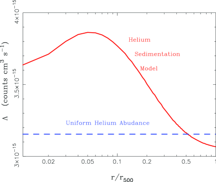
Figure 1: The band-averaged X-ray cooling function, $\Lambda_{ee}(r)$, for two different helium distributions in the ICM: a uniform helium abundance (blue dashed line) and a helium sedimentation distribution provided by Peng & Nagai (2009) (red line). The overdensity radius $r_{500}$ is the radius within which the mean cluster density is a factor of 500 times greater than the critical density of the universe at the cluster redshift.

2.2 Application of Cluster Models to X-ray Data

We start with the projected surface brightness (Birkinshaw et al., 1991; Hughes & Birkinshaw, 1998):

$$S_{x}=\frac{1}{4\pi(1+z)^{3}}\int n_{e}^{2}\ \Lambda_{ee}\ d\ell,$$ (1)

where $S_{x}$ is in detector units (counts s^-1 cm^-2 arcmin^-2), $\Lambda_{ee}$ is the band averaged X-ray cooling function in counts cm³ s^-1, $n_{e}$ is the number density of electrons, z is the redshift, and the integral is along the line of sight, $\ell$.

We calculate the X-ray cooling function in two limiting cases: (i) a uniform abundance (Anders & Grevesse, 1989) and (ii) the radial abundance profile of Peng & Nagai (2009) obtained for a sedimentation time scale of 11 Gyr with no magnetic field. We use the astrophysical plasma emission database (APED) which includes thermal bremsstrahlung, radiative recombination, line emission, and two-photon emission (Smith et al., 2001). In addition, we apply corrections for galactic absorption (Morrison & McCammon, 1983), relativistic effects (Itoh et al., 2000), and electron-electron bremsstrahlung (Itoh et al., 2001), to obtain the X-ray emissivity ($\epsilon_{\nu}$) as a function of frequency $\nu$.

The band-averaged X-ray cooling function ($\Lambda_{ee}(T,r)$) is obtained by integrating the $\epsilon_{\nu}$ over the observed Chandra energy band (0.7-7.0 keV):

$$\Lambda_{ee}(T,r)=\frac{\int_{\nu}\epsilon_{\nu}d\nu}{n_{e}^{2}}.$$ (2)

The resulting band-averaged X-ray cooling function for a uniform abundance (Anders & Grevesse, 1989) and a helium sedimentation profile (Peng & Nagai, 2009) is shown in Figure 1.

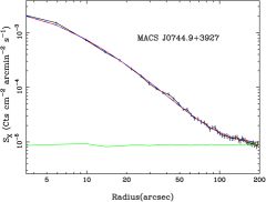
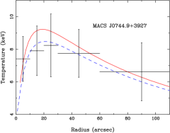
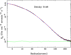
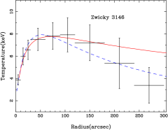
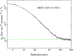
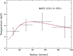
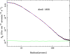
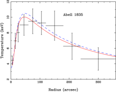
Figure 2: X-ray surface brightness (left column) and temperature profiles (right column) for the sample of eight relaxed galaxy clusters. The black points are derived from the X-ray image and spectroscopic data. The blue lines in both profiles show the best fit model to the data obtained using a uniform Anders & Grevesse (1989) helium abundance, and the red lines show the best fit model obtained using the Peng & Nagai (2009) helium sedimentation distribution; the green lines in surface brightness profiles indicate the background levels determined from the blank sky observations. The overall $\chi^{2}$ of the fits obtained from the uniform helium abundance and the helium sedimentation model (Tables LABEL:table:bestFitParams_A&G and LABEL:table:bestFitParams_P&N) show that both distributions give equally good fits to Chandra data.

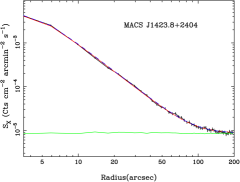
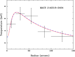
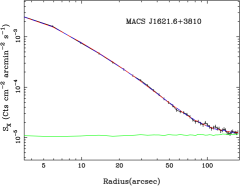
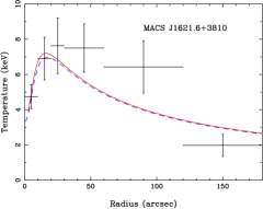
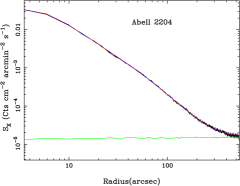
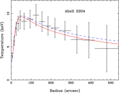
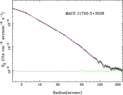
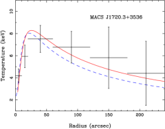
Figure 2: X-ray surface brightness and temperature profiles for our sample of galaxy clusters (cont’d).

To obtain the electron number density $n_{e}(r)$ and temperature $T(r)$ profiles, we apply the analytic model for the intra-cluster plasma developed by Bulbul et al. (2010) and compare the model predictions to the observed surface brightness and temperature data points found in §2.1.

The electron number density is

$$n_{e}(r)= n_{e0}\left(\frac{1}{(\beta-2)}\frac{(1+r/r_{s})^{\beta-2}-1}{r/r_{s}(1+r/r_{s})^{\beta-2}}\right)^{n}\tau_{cool}^{-1}(r)$$ (3)

where $n_{e0}$ is the central value of the number density of electrons, $r_{s}$ is the scaling radius, $\beta+1$ is the slope of the total matter density profile, and n is the polytropic index. $\tau_{cool}(r)$ is the phenomenological core-taper function used for cool-core clusters (Vikhlinin et al., 2006),

$$\tau_{cool}(r)=\frac{\alpha+(r/r_{cool})^{\gamma}}{1+(r/r_{cool})^{\gamma}}.$$ (4)

The corresponding Bulbul et al. (2010) temperature profile is

$$T(r)= T_{0}\left(\frac{1}{(\beta-2)}\frac{(1+r/r_{s})^{\beta-2}-1}{r/r_{s}(1+r/r_{s})^{\beta-2}}\right)\tau_{cool}(r)$$ (5)

where $T_{0}$ is the normalization parameter, and the other parameters are in common with those in Equation 3.

We vary the model parameters using a Monte Carlo Markov Chain approach (Bonamente et al., 2004; Bulbul et al., 2010); the best fit model parameters for a uniform helium abundance and a helium sedimentation scenario are given in Table LABEL:table:bestFitParams_P&N and are shown by the solid blue and red curves in Figure 2. We assume that clusters with redshift z $>$ 0.3 have $\beta=2$, since the polytropic index (n) and $\beta$ cannot be determined simultaneously from the data available. For all of the clusters we use a core taper parameter $\gamma=2.0$ except for Zwicky 3146, for which we obtained a better fit with $\gamma=1.0$. With these choices of fixed parameters, we obtain acceptable fits to the data for both the assumed uniform and sedimented helium profiles (see Tables LABEL:table:bestFitParams_A&G and LABEL:table:bestFitParams_P&N).

2.3 Cluster Mass

The gas mass is the volumetric integral of the number density of electrons multiplied by the electron mean molecular weight:

$$M_{gas}(r)=m_{p}\int_{V}\mu_{e}(r)\ n_{e}(r)\ dV,$$ (6)

where $m_{p}$ is the proton mass and $n_{e}(r)$ is defined in Equation 3. Since the mean molecular weight of electrons $\mu_{e}(r)$ is dependent on the ion distribution in the plasma, we use the same approach as in the X-ray cooling function calculations to determine its radial distribution. The electron mean molecular weight $\mu_{e}(r)$ , which is calculated for a uniform helium abundance (Anders & Grevesse, 1989) and the radial helium abundance profile of (Peng & Nagai, 2009) obtained for a sedimentation timescale of 11 Gyr with no magnetic field, is shown in the top panel of Figure 3.

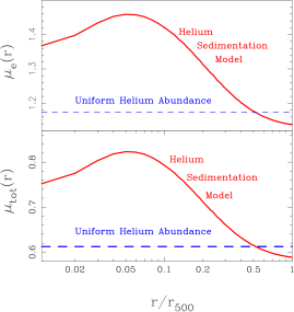
Figure 3: The distributions of the electron mean molecular weight (top panel) and the total mean molecular weight (bottom panel) as a function of radius for a uniform Anders & Grevesse (1989) helium abundance (blue dashed line) and for the 11 Gyr helium sedimentation model Peng & Nagai (2009)(red line).

Similarly, the total mass is the volumetric integral of the total matter density $\rho_{tot}(r)$,

$$M_{tot}(r)=\int_{V}\ \rho_{tot}(r)\ dV.$$ (7)

As in Bulbul et al. (2010), the total matter density is found by

$$\rho_{tot}(r)=\left[\frac{T_{0}k(n+1)(\beta-1)}{4\pi Gm_{p}r_{s}^{2}}\right]\frac{1}{\mu_{tot}(r)}\frac{1}{(1+r/r_{s})r/r_{s}}.$$ (8)

where $k$ is the Boltzmann constant, $G$ is Newton’s gravitational constant, and $\mu_{tot}(r)$ is the total mean molecular weight, which is also dependent on the ion distribution in the plasma. The total mean molecular weight, $\mu_{tot}(r)$ is calculated assuming a uniform helium distribution and the helium sedimentation model (see Figure 3 bottom panel) as was done for the $\mu_{e}$ calculations.

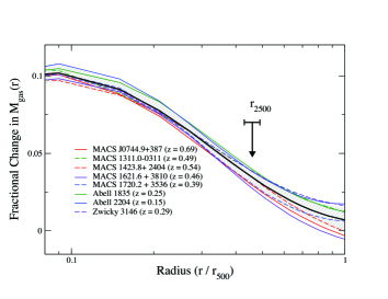
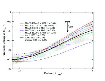
Figure 4: The fractional change in gas mass and total mass with radius as a result of an extreme helium sedimentation with respect to masses produced by a uniform Anders & Grevesse (1989) helium abundance for a sample of eight relaxed clusters. The black lines correspond to the mean fractional change and the shaded are indicates the standard deviation of the fractional change in gas mass and total mass measurements.

3 Results

We measure cluster masses and scaling relations assuming the limiting cases of uniform helium abundance (Anders & Grevesse, 1989) and the radially-varying, sedimented helium abundance profile of Peng & Nagai (2009) described in Section 2.2.

In order to determine the fractional change in cluster mass measurements introduced by the spatial variation in the helium distribution, we calculate gas mass and total mass for each helium abundance model. Gas mass is calculated using Equation 6 and the electron mean molecular weight distributions shown in the top panel of Figure 3. The total mass is calculated using Equation 7 and the total mean molecular weight distributions shown in the bottom panel of Figure 3. The gas mass and total mass at $r_{2500}$ and $r_{500}$ are given in Tables LABEL:table:masses_A&G and LABEL:table:masses_P&N for both the uniform helium abundance and the sedimented case.

Table 2: Best-fit Parameters of the Bulbul et al. (2010) Model Produced Using a Uniform helium Abundance Model (Anders & Grevesse, 1989)

Cluster	$n_{e0}$	$r_{s}$	$n$	$\beta$	$T_{0}$	$r_{cool}$	$\alpha$	$\gamma$	$\chi^{2}$ (d.o.f.)	P value
	($10^{-2}cm^{-3}$)	(arcsec)			($keV$)	(arcsec)
MACS J0744.9+3927	2.13${}^{+0.69}_{-0.30}$	13.64${}^{+2.14}_{-3.18}$	2.77${}^{+0.15}_{-0.18}$	2.0	22.47${}^{+3.73}_{-1.39}$	15.99${}^{+4.56}_{-3.82}$	0.13${}^{+0.08}_{-0.02}$	1.0	44.3 (51)	73.5%
Zwicky 3146	1.27${}^{+0.43}_{-0.06}$	52.99${}^{+5.47}_{-5.43}$	2.58${}^{+0.83}_{-0.77}$	2.85${}^{+0.83}_{-0.18}$	30.02${}^{+1.99}_{-2.31}$	58.95${}^{+5.99}_{-6.07}$	0.06${}^{+0.02}_{-0.02}$	1.0	66.8 (78)	81.2%
MACS J1311.0-0311	1.73${}^{+0.20}_{-0.65}$	40.32${}^{+5.69}_{-6.31}$	5.38${}^{+3.19}_{-0.47}$	2.0	11.36${}^{+1.46}_{-0.71}$	20.73${}^{+4.36}_{-1.36}$	0.33${}^{+0.04}_{-0.13}$	2.0	70.56 (63)	42.5 %
Abell 1835	2.57${}^{+0.29}_{-0.07}$	40.32${}^{+3.29}_{-6.48}$	3.98${}^{+0.73}_{-0.41}$	1.94${}^{+0.15}_{-0.22}$	18.26${}^{+0.42}_{-1.61}$	22.65${}^{+0.28}_{-1.17}$	0.18${}^{+0.02}_{-0.01}$	2.0	99.3 (93)	30.8%
MACS J1423.8+2404	3.29${}^{+0.68}_{-0.29}$	11.39${}^{+1.60}_{-2.17}$	2.98${}^{+0.14}_{-0.16}$	2.0	16.03${}^{+1.00}_{-1.32}$	13.07${}^{+0.63}_{-0.73}$	0.18${}^{+0.04}_{-0.02}$	2.0	45.5 (50)	65.3%
MACS J1621.6+3810	2.84${}^{+0.62}_{-0.16}$	14.39${}^{+3.85}_{-2.85}$	3.12${}^{+0.17}_{-0.12}$	2.0	12.63${}^{+0.95}_{-0.97}$	9.01${}^{+0.73}_{-0.86}$	0.26${}^{+0.05}_{-0.03}$	2.0	32.4 (45)	92.1%
Abell 2204	4.42${}^{+0.37}_{-0.24}$	21.73${}^{+1.50}_{-2.01}$	6.44${}^{+1.02}_{-0.51}$	1.39${}^{+0.04}_{-0.06}$	14.28${}^{+0.75}_{-0.78}$	19.42${}^{+0.60}_{-0.73}$	0.16${}^{+0.01}_{-0.01}$	2.0	115.5 (145)	96.6%
MACS J1720.3+3536	2.12${}^{+0.24}_{-0.20}$	31.69${}^{+5.58}_{-5.03}$	3.97${}^{+0.29}_{-0.27}$	2.0	13.01${}^{+0.97}_{-0.79}$	10.95${}^{+0.86}_{-0.80}$	0.13${}^{+0.02}_{-0.01}$	2.0	46.5 (60)	89.9%

Table 3: Best-fit Parameters of the Bulbul et al. (2010) Produced Using a helium Sedimentation Model (Peng & Nagai, 2009)

Cluster	$n_{e0}$	$r_{s}$	$n$	$\beta$	$T_{0}$	$r_{cool}$	$\alpha$	$\gamma$	$\chi^{2}$ (d.o.f.)	P value
	($10^{-2}cm^{-3}$)	(arcsec)			($keV$)	(arcsec)
MACS J0744.9+3927	2.07${}^{+0.26}_{-0.25}$	14.79${}^{+1.37}_{-1.88}$	2.84${}^{+0.10}_{-0.15}$	2.0	21.75${}^{+1.71}_{-1.91}$	12.19${}^{+3.51}_{-2.24}$	0.13	1.0	45.7 (52)	71.85%
Zwicky 3146	1.28${}^{+0.10}_{-0.07}$	51.37${}^{+7.53}_{-5.16}$	2.68${}^{+0.39}_{-0.24}$	2.68${}^{+0.37}_{-0.13}$	25.92${}^{+1.88}_{-0.91}$	47.33${}^{+3.63}_{-5.62}$	0.11	1.0	60.83 (79)	93.6%
MACS J1311.0-0311	1.56${}^{+0.07}_{-0.09}$	42.26${}^{+6.41}_{-7.56}$	5.38${}^{+0.54}_{-0.67}$	2.0	10.91${}^{+1.01}_{-0.76}$	19.32${}^{+1.94}_{-1.16}$	0.34	2.0	44.6 (64)	68.9%
Abell 1835	2.36${}^{+0.30}_{-0.05}$	38.75${}^{+5.10}_{-1.18}$	4.01${}^{+0.28}_{-0.83}$	2.88${}^{+0.35}_{-0.29}$	17.75${}^{+0.91}_{-0.16}$	21.43${}^{+0.42}_{-0.39}$	0.18	2.0	108.1 (94)	13.6 %
MACS J1423.8+2404	2.99${}^{+0.11}_{-0.09}$	11.73${}^{+0.86}_{-0.84}$	2.93${}^{+0.11}_{-0.54}$	2.0	15.49${}^{+0.98}_{-1.28}$	12.28${}^{+0.45}_{-0.54}$	0.18	2.0	47.2 (51)	58.5 %
MACS J1621.6+3810	2.58${}^{+0.16}_{-0.14}$	14.61${}^{+1.10}_{-1.26}$	3.06${}^{+0.09}_{-0.12}$	2.0	12.66${}^{+0.95}_{-1.18}$	8.29${}^{+0.69}_{-0.62}$	0.26	2.0	33.88 (46)	88.8 %
Abell 2204	4.15${}^{+0.07}_{-0.08}$	19.81${}^{+0.43}_{-0.56}$	5.59${}^{+0.66}_{-0.39}$	2.43${}^{+0.04}_{-0.05}$	14.51${}^{+0.53}_{-0.59}$	18.81${}^{+0.39}_{-0.28}$	0.16	2.0	127.7 (146)	84.6 %
MACS J1720.3+3536	1.91${}^{+0.13}_{-0.12}$	31.62${}^{+3.71}_{-5.30}$	3.85${}^{+0.21}_{-0.19}$	2.0	12.96${}^{+1.01}_{-0.79}$	10.57${}^{+0.66}_{-0.63}$	0.13	2.0	47.3(61)	90.0%

Table 4: Gas Mass and Total Mass for the Uniform helium Abundance Model at the Overdensity Radii $r_{2500}$ and $r_{500}$

Cluster	$r_{2500}$	$M_{gas}(r_{2500})$	$M_{tot}(r_{2500})$	$r_{500}$	$M_{gas}(r_{500})$	$M_{tot}(r_{500})$
	(arcsec)	($10^{13}M_{\odot}$)	($10^{14}M_{\odot}$)	(arcsec)	($10^{13}M_{\odot}$)	($10^{14}M_{\odot}$)
MACS J0744.9+3927	57.9${}^{+3.1}_{-2.8}$	2.98${}^{+0.23}_{-0.20}$	2.07${}^{+0.36}_{-0.29}$	120.2${}^{+8.1}_{-6.8}$	8.78${}^{+0.66}_{-0.55}$	3.69${}^{+0.80}_{-0.59}$
Zwicky 3146	127.6${}^{+4.5}_{-5.3}$	4.26${}^{+0.18}_{-0.20}$	3.17${}^{+0.35}_{-0.38}$	266.7${}^{+12.4}_{-14.2}$	9.72${}^{+0.39}_{-0.44}$	5.78${}^{+1.23}_{-1.10}$
MACS J1311.0-0311	78.7${}^{+5.9}_{-5.5}$	2.29${}^{+0.19}_{-0.18}$	2.51${}^{+0.61}_{-0.49}$	173.1${}^{+17.1}_{-15.1}$	5.16${}^{+0.29}_{-0.29}$	5.34${}^{+1.74}_{-1.28}$
Abell 1835	150.6${}^{+3.4}_{-4.2}$	4.97${}^{+0.14}_{-0.17}$	3.72${}^{+0.26}_{-0.30}$	309.7${}^{+9.8}_{-13.1}$	12.08${}^{+0.38}_{-0.50}$	6.38${}^{+0.64}_{-0.79}$
MACS J1423.8+2404	63.4${}^{+2.4}_{-2.8}$	2.16${}^{+0.10}_{-0.11}$	1.61${}^{+0.19}_{-0.21}$	125.9${}^{+5.4}_{-6.4}$	5.46${}^{+0.23}_{-0.27}$	2.52${}^{+0.34}_{-0.37}$
MACS J1621.6+3810	67.8${}^{+4.2}_{-3.5}$	1.78${}^{+0.15}_{-0.12}$	1.37${}^{+0.27}_{-0.20}$	135.1${}^{+9.3}_{-7.8}$	4.77${}^{+0.31}_{-0.26}$	2.17${}^{+0.48}_{-0.35}$
Abell 2204	225.7${}^{+4.1}_{-4.1}$	3.99${}^{+0.09}_{-0.09}$	3.37${}^{+0.19}_{-0.18}$	479.8${}^{+11.4}_{-11.2}$	10.35${}^{+0.26}_{-0.26}$	6.48${}^{+0.47}_{-0.44}$
MACS J1720.3+3536	91.6${}^{+4.2}_{-3.9}$	2.82${}^{+0.18}_{-0.16}$	2.34${}^{+0.34}_{-0.28}$	190.5${}^{+10.6}_{-9.3}$	7.38${}^{+0.35}_{-0.33}$	4.20${}^{+0.74}_{-0.59}$

Table 5: Gas Mass and Total Mass for the helium Sedimentation Model at the Overdensity Radii $r_{2500}$ and $r_{500}$

Cluster	$r_{2500}$	$M_{gas}(r_{2500})$	$M_{tot}(r_{2500})$	$r_{500}$	$M_{gas}(r_{500})$	$M_{tot}(r_{500})$
	(arcsec)	($10^{13}M_{\odot}$)	($10^{14}M_{\odot}$)	(arcsec)	($10^{13}M_{\odot}$)	($10^{14}M_{\odot}$)
MACS J0744.9+3927	53.9${}^{+2.7}_{-3.1}$	2.75${}^{+0.21}_{-0.22}$	1.66${}^{+0.27}_{-0.27}$	116.9${}^{+6.0}_{-6.9}$	8.43${}^{+0.50}_{-0.54}$	3.41${}^{+0.56}_{-0.56}$
Zwicky 3146	116.0${}^{+4.2}_{-3.7}$	3.94${}^{+0.17}_{-0.15}$	2.38${}^{+0.27}_{-0.22}$	246.5${}^{+13.1}_{-11.5}$	9.14${}^{+0.44}_{-0.38}$	4.56${}^{+0.77}_{-0.61}$
MACS J1311.0-0311	71.2${}^{+3.9}_{-4.3}$	2.12${}^{+0.12}_{-0.15}$	1.86${}^{+0.32}_{-0.32}$	165.6${}^{+9.2}_{-10.5}$	5.06${}^{+0.16}_{-0.19}$	4.67${}^{+0.82}_{-0.83}$
Abell 1835	138.6${}^{+2.6}_{-4.3}$	4.62${}^{+0.10}_{-0.17}$	2.89${}^{+0.16}_{-0.26}$	294.8${}^{+7.7}_{-12.7}$	11.59${}^{+0.30}_{-0.51}$	5.58${}^{+0.45}_{-0.69}$
MACS J1423.8+2404	58.8${}^{+2.4}_{-2.2}$	2.01${}^{+0.10}_{-0.01}$	1.29${}^{+0.17}_{-0.14}$	120.9${}^{+4.8}_{-4.2}$	5.20${}^{+0.19}_{-0.18}$	2.23${}^{+0.27}_{-0.23}$
MACS J1621.6+3810	63.4${}^{+3.4}_{-3.4}$	1.65${}^{+0.11}_{-0.11}$	1.12${}^{+0.19}_{-0.17}$	130.7${}^{+6.9}_{-6.8}$	4.55${}^{+0.23}_{-0.23}$	1.97${}^{+0.33}_{-0.29}$
Abell 2204	201.0${}^{+3.6}_{-3.9}$	3.55${}^{+0.08}_{-0.09}$	2.38${}^{+0.13}_{-0.14}$	440.4${}^{+11.5}_{-10.9}$	9.53${}^{+0.28}_{-0.25}$	5.01${}^{+0.40}_{-0.36}$
MACS J1720.3+3536	84.6${}^{+3.9}_{-3.5}$	2.59${}^{+0.16}_{-0.15}$	1.84${}^{+0.27}_{-0.22}$	182.9${}^{+8.5}_{-8.1}$	7.09${}^{+0.31}_{-0.29}$	3.72${}^{+0.54}_{-0.47}$

Table 6: Percentage Changes in $M_{gas}$ and $M_{tot}$

Region	% Change in Mgas	% Change in Mtot
$0.0<r<0.1r_{500}$	10.5 $\pm$ 0.8	25.1 $\pm$ 1.1
$0.0<r<r_{2500}$	3.5 $\pm$ 1.0	13.9 $\pm$ 3.1
$0.0<r<r_{500}$	1.4 $\pm$ 1.2	12.5 $\pm$ 5.5

The fractional change with radius in gas mass and total mass measurements as a result of an extreme helium sedimentation case is shown in Figure 4 for each of the relaxed galaxy clusters in our sample. The black line shows the mean fractional change in gas mass (left panel) and total mass (right panel). The shaded areas indicate the standard deviations of the gas mass and total mass inferred for the sample. In Table 6 we show the weighted mean percentage difference with rms errors in gas mass and total mass measurements within small cluster radius ($r<0.1r_{500}$), intermediate radius ($r<r_{2500}$) and large radius ($r<r_{500}$). On average, at large radii ($r<r_{500}$) the effect of helium sedimentation on gas mass is negligible (1.3 $\pm$ 1.2 %). The helium sedimentation model produces an average of 10.2 $\pm$ 5.5 % decrease in the inferred total mass within $r_{500}$. Significantly stronger effects in the gas mass (10.5 $\pm$ 0.8 %) and total mass (25.1 $\pm$ 1.1 %) are seen at small cluster radii ($r<0.1r_{500}$) where the helium abundance enhancement and gradient are greater. This result is in agreement with the expected change in the mass measurements predicted by theoretical studies (Qin & Wu, 2000; Peng & Nagai, 2009).

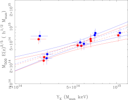
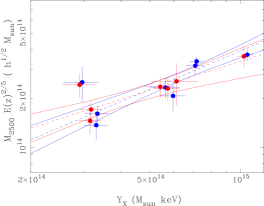
Figure 5: The Y_X-M₅₀₀ and Y_X-M₂₅₀₀ scaling relations for a sample of eight relaxed galaxy clusters. The blue data points and curves correspond to the measurements obtained from a uniform helium abundance case and red data points and curves correspond to the measurements obtained from a helium sedimentation model. The dashed lines show the best fit power law relation and solid curves show the 90% confidence levels.

3.1 $Y_{X}$-$M$ Scaling Relation

We examine the effect of helium sedimentation on the cluster mass scaling relations. The X-ray mass proxy, $Y_{X}$, is defined as (Kravtsov et al., 2006),

$$Y_{X}=M_{gas}(r_{500})\ T_{X}.$$ (9)

where $T_{X}$ is the mean X-ray spectroscopic temperature measured within $r_{500}$ (Kravtsov et al., 2006; Vikhlinin et al., 2009). The importance of this quantity is that there is a correlation between $Y_{X}$ and the total cluster mass, $M_{500}$ (Kravtsov et al., 2006; Vikhlinin et al., 2009) and this correlation motivates $Y_{X}$ as a proxy for total mass (Vikhlinin et al., 2009; Andersson et al., 2010). In this section we investigate the effect of helium sedimentation on the $Y_{X}$-$M_{\Delta}$ scaling relation at overdensities $\Delta=(2500,500)$ (i.e. for properties computed within $r<(r_{2500},r_{500})$).

The $Y_{X}$-$M_{500}$ scaling relation is found using gas mass and total mass measurements shown in Tables LABEL:table:masses_A&G and LABEL:table:masses_P&N for a uniform helium abundance and helium sedimentation distributions. The average spectral temperature $T_{X}$ is obtained with a single-temperature thermal plasma model (APEC) fit to the Chandra spectrum in the radial range $0.15r_{500}<r<r_{500}$. Using the XSPEC analysis package to vary the helium abundance assumed in our spectroscopic fits, we determine that the assumed helium distribution has a negligible effect ($\lesssim$ 1%) on the measurements of the average X-ray spectral temperatures $T_{X}$. We report the average X-ray temperature $T_{X}$ and the X-ray mass proxy $Y_{X}$ for a uniform helium distribution and helium sedimentation model in Table 7.

Table 7: Measured Average Temperature ($T_{X}$) and the Mass Proxy ($Y_{X}$)

Cluster	$T_{X}$	$Y_{X}$	$Y_{X}$
		(Uniform heliumAbundance)	( helium Sedimentation)
	(keV)	($10^{14}keVM_{\odot}$)	($10^{14}keVM_{\odot}$)
MACS J0744.9+3927	6.80 $\pm$ 0.5	5.97 $\pm$ 0.58	5.73 $\pm$ 0.54
Zwicky 3146	7.29 $\pm$ 0.4	7.09 $\pm$ 0.48	6.66 $\pm$ 0.45
MACS J1311.0-0311	5.75 $\pm$ 0.7	2.97 $\pm$ 0.39	2.91 $\pm$ 0.37
Abell 1835	8.79 $\pm$ 0.3	10.57 $\pm$ 0.49	10.30 $\pm$ 0.50
MACS J1423.8+2404	6.11 $\pm$ 0.5	3.34 $\pm$ 0.31	3.18 $\pm$ 0.27
MACS J1621.6+3810	6.93 $\pm$ 0.5	3.31 $\pm$ 0.29	3.15 $\pm$ 0.27
Abell 2204	6.91 $\pm$ 0.3	7.16 $\pm$ 0.36	6.63 $\pm$ 0.34
MACS J1720.3+3536	7.63 $\pm$ 0.8	5.63 $\pm$ 0.64	5.41 $\pm$ 0.61

The $Y_{X}$-$M_{500}$ scaling relation for our sample of eight relaxed galaxy clusters is shown in Figure 5 (left panel). For each $\Delta$, we fit the $Y_{X}$-$M_{\Delta}$ data using a power law relation (Vikhlinin et al., 2009),

$$M_{\Delta}\ E(z)^{2/5} =a\left(\frac{Y_{X}}{3\times 10^{14}M_{\odot}keV}\right)^{b}\ h^{1/2}M_{\odot},$$ (10)

where $a$ is the normalization, $b$ is the slope, and $E(z)$ is the evolution function. The best fit normalizations and slopes are reported in Table 8 with the goodness of the fit. In Figure 5 the dashed lines shows the best fit power law model and solid lines shows the 90 % confidence intervals for both a uniform helium abundance and the helium sedimentation cases.

From the $Y_{X}$-$M_{500}$ fit to the data on the eight galaxy clusters in our sample, we conclude that both the uniform and sedimented helium fits are statistically consistent with the power law slope found by Vikhlinin et al. (2009) (see Table 8). helium sedimentation changes the normalization by 10 $\pm$ 0.9 % at $r_{500}$. The difference in best-fit slope between the uniform and helium sedimentation models is small compared to the statistical uncertainty.

We also investigate the effect of helium sedimentation on the Y_X-$M_{2500}$ scaling relation. Figure 5 (right panel) shows the $Y_{X}$-$M_{2500}$ scaling relation for our sample. We fit the $Y_{X}$-$M_{2500}$ scaling relation data with a power law shown in Equation 10. The dashed lines show the best fit power law relation with the goodness of fit reported in Table 9 for the uniform and sedimented helium profiles. In Figure 5 the best fit power law model is shown in dashed line and 90% confidence levels are shown in solid lines for both uniform helium abundance and helium sedimentation models.

The self-similar $Y_{X}-M_{2500}$ scaling relation discussed by Bonamente et al. (2008) is of the form:

$$Y_{X}\propto M_{2500}^{5/3}E(z)^{2/3}$$ (11)

which is equivalent to the $Y_{X}-M_{2500}$ scaling relation form we use for this work

$$M_{2500}E(z)^{2/5}\propto Y_{X}^{3/5}.$$ (12)

Recently, Bonamente et al. (2008) measured the $Y_{X}-M_{2500}$ scaling relation, and found it to be consistent with the self-similar prediction, $b=1.66\pm 0.20$ in Equation 10. In our fit $Y_{X}-M_{2500}$ (shown in Table 9), we also find that both the uniform helium abundance and the helium sedimentation cases are consistent with the slope measured by Bonamente et al. (2008) and with the self-similar expectation (Equation 12). The difference in best-fit slopes $b$ is negligible compared to the statistical uncertainty reported in Table 9. However, we find that helium sedimentation affects the normalization of the $Y_{X}-M_{2500}$ scaling relation by 13 $\pm$ 0.6 %.

Table 8: Comparison of Normalization and Slope of the $Y_{X}-M_{500}$ Scaling Relation

	a	b	$\chi^{2}$ (d.o.f)	P (%)
	($10^{14}\ h^{1/2}\ M_{\odot}$)
Uniform helium Abundance	3.12 $\pm$ 0.87	0.83 $\pm$ 0.42	8.6 (6)	19.7
helium Sedimentation Model	2.92$\pm$ 0.61	0.77 $\pm$ 0.22	10.7 (6)	9.8

Table 9: Comparison of Normalization and Slope of the $Y_{X}-M_{2500}$ Scaling Relation

	a	b	$\chi^{2}$(d.o.f.)	P
	($10^{14}\ h^{1/2}\ M_{\odot}$)
Uniform helium Abundance	1.94 $\pm$ 0.50	0.72 $\pm$ 0.28	5.0 (6)	54.3
helium Sedimentation Model	1.66 $\pm$ 0.30	0.66 $\pm$ 0.11	5.6 (6)	46.9

4 Conclusion

In this paper we investigate the upper limits to the effect of the helium sedimentation on X-ray derived cluster masses and the $Y_{X}-M_{500}$ and $Y_{X}-M_{2500}$ scaling relations using Chandra X-ray observations of eight relaxed galaxy clusters. We used a limiting helium sedimentation profile for 11 Gyr old clusters based on the simulations performed by Peng & Nagai (2009) and compare these results with those assuming a uniform helium distribution in order to determine the maximum impact of helium sedimentation. This work is the first application of a theoretically predicted helium sedimentation profile to Chandra observations. We fit the deep exposure Chandra X-ray spectroscopic and imaging data of the eight relaxed galaxy clusters with an analytic model of the intra-cluster plasma developed by Bulbul et al. (2010). We demonstrated that both a uniform helium and a limiting helium sedimentation model can accurately describe the surface brightness and temperature profiles obtained from the Chandra X-ray data.

We have found that, on average, the effect of helium sedimentation on gas mass inferred within large radii ($r<r_{500}$) is negligible (1.3 $\pm$ 1.2 %). The helium sedimentation model produces a 10.2 $\pm$ 5.5 % mean decrease in the total mass inferred within $r<r_{500}$. Significantly stronger effects in the gas mass (10.5 $\pm$ 0.8 %) and total mass (25.1 $\pm$ 1.1 %) are seen at small radii owing to a larger variance in helium abundance in the inner region, $r\leq 0.1\,r_{500}$. This study supports the view that helium sedimentation should have a negligible impact on cluster mass inferred within large radii. This result is consistent with the predictions of the previous theoretical studies by Ettori & Fabian (2006) and Peng & Nagai (2009).

The fractional change in both the gas mass and the total mass measurements due to helium sedimentation do not show any trend with redshift. The strongest effect on the cluster total mass is observed on an intermediate redshift cluster, Zwicky 3146, while the smallest effect is observed on the highest redshift cluster in the sample, MACS J0744.9+3827.

In order to investigate the effect of helium sedimentation on the best-fit slopes and normalizations of the $Y_{X}-M_{500}$ and $Y_{X}-M_{2500}$ scaling relations, we used gas mass measurements, and the mean X-ray spectroscopic temperature $T_{X}$ to estimate the X-ray mass proxy $Y_{X}$ for both the uniform and sedimented helium abundance profiles. Both uniform and helium sedimentation models produce slopes which are statistically consistent with the power law slopes found by Bonamente et al. (2008) and Vikhlinin et al. (2009). We have found that helium sedimentation has a negligible effect on the slopes of $Y_{X}-M_{500}$ and $Y_{X}-M_{2500}$ scaling relations. We have also found that helium sedimentation changes the normalization of the $Y_{X}-M_{500}$ scaling relation by 10 $\pm$ 0.9 % and the $Y_{X}-M_{2500}$ scaling relation by 13 $\pm$ 0.6 %.

References

- Abramopoulos et al. (1981) Abramopoulos, F., Chanan, G. A., & Ku, W. H.-M. 1981, ApJ, 248, 429
- Allen et al. (2008) Allen, S. W., Rapetti, D. A., Schmidt, R. W., Ebeling, H., Morris, R. G., & Fabian, A. C. 2008, MNRAS, 383, 879
- Anders & Grevesse (1989) Anders, E., & Grevesse, N. 1989, Geochim. Cosmochim. Acta., 53, 197
- Andersson et al. (2010) Andersson, K., et al. 2010, arXiv:1006.3068
- Birkinshaw et al. (1991) Birkinshaw, M., Hughes, J. P., & Arnaud, K. A. 1991, ApJ, 379, 466
- Bonamente et al. (2004) Bonamente, M., Joy, M. K., Carlstrom, J. E., Reese, E. D., & LaRoque, S. J. 2004, ApJ, 614, 56
- Bonamente et al. (2006) Bonamente, M., Joy, M. K., LaRoque, S. J., Carlstrom, J. E., Reese, E. D., & Dawson, K. S. 2006, ApJ, 647, 25
- Bonamente et al. (2008) Bonamente, M., Joy, M., LaRoque, S. J., Carlstrom, J. E., Nagai, D., & Marrone, D. P. 2008, ApJ, 675, 106
- Bulbul et al. (2010) Bulbul, G. E., Hasler, N., Bonamente, M., & Joy, M. 2010, ApJ, 720, 1038
- Chuzhoy & Nusser (2003) Chuzhoy, L., & Nusser, A. 2003, MNRAS, 342, L5
- Chuzhoy & Loeb (2004) Chuzhoy, L., & Loeb, A. 2004, MNRAS, 349, L13
- Ettori & Fabian (2006) Ettori, S., & Fabian, A. C. 2006, MNRAS, 369, L42
- Fabian & Pringle (1977) Fabian, A. C., & Pringle, J. E. 1977, MNRAS, 181, 5P
- Gilfanov & Sunyaev (1984) Gilfanov, M. R., & Sunyaev, R. A. 1984, Pis ma Astronomicheskii Zhurnal, 10, 329
- Hasler et al. (2011) Hasler, N. et al. 2010, in prep.
- Hughes & Birkinshaw (1998) Hughes, J. P., & Birkinshaw, M. 1998, ApJ, 501, 1
- Itoh et al. (2000) Itoh, N., Sakamoto, T., Kusano, S., Nozawa, S., & Kohyama, Y. 2000, ApJS, 128, 125
- Itoh et al. (2001) Itoh, N., Kawana, Y., & Nozawa, S. 2001, arXiv:astro-ph/0111040
- Kalberla et al. (2005) Kalberla, P. M. W., Burton, W. B., Hartmann, D., Arnal, E. M., Bajaja, E., Morras, R., Poumlppel, W. G. L. 2005, A&A, 440, 775
- Kravtsov et al. (2006) Kravtsov, A. V., Vikhlinin, A., & Nagai, D. 2006, ApJ, 650, 128
- Mantz et al. (2010) Mantz, A., Allen, S. W., Ebeling, H., Rapetti, D., & Drlica-Wagner, A. 2010, MNRAS, 406, 1773
- Markevitch et al. (2003) Markevitch, M. et al. 2003, ApJ, 583, 70
- Markevitch (2007) Markevitch, M. 2007, arXiv:0705.3289
- Morrison & McCammon (1983) Morrison, R., & McCammon, D. 1983, ApJ, 270, 119
- Peng & Nagai (2009) Peng, F., & Nagai, D. 2009, ApJ, 693, 839
- Qin & Wu (2000) Qin, B., & Wu, X.-P. 2000, ApJ, 529, L1
- Reese et al. (2000) Reese, E. D., et al. 2000, ApJ, 533, 38
- Rephaeli (1978) Rephaeli, Y. 1978, ApJ, 225, 335
- Shtykovskiy & Gilfanov (2010) Shtykovskiy, P., & Gilfanov, M. 2010, MNRAS, 401, 1360
- Smith et al. (2001) Smith, R. K., Brickhouse, N. S., Liedahl, D. A., & Raymond, J. C. 2001, ApJ, 556, L91
- Vikhlinin et al. (2006) Vikhlinin, A., Kravtsov, A., Forman, W., Jones, C., Markevitch, M., Murray, S. S., & Van Speybroeck, L. 2006, ApJ, 640, 691
- Vikhlinin et al. (2009) Vikhlinin, A. et al. 2009, ApJ, 692, 1060