Nonlocality of a single photon: paths to an EPR-steering experiment

Abstract

A single photon incident on a beam splitter produces an entangled field state, and in principle could be used to violate a Bell-inequality, but such an experiment (without post-selection) is beyond the reach of current experiments. Here we consider the somewhat simpler task of demonstrating EPR-steering with a single photon (also without post-selection). That is, of demonstrating that Alice’s choice of measurement on her “half” of a single photon can affect the other “half” of the photon in Bob’s lab, in a sense rigorously defined by us and Doherty [Phys. Rev. Lett. 98, 140402 (2007)]. Previous work by Lvovsky and co-workers [Phys. Rev. Lett. 92, 047903 (2004)] has addressed this phenomenon (which they called “remote preparation”) experimentally using homodyne measurements on a single photon. Here we show that, unfortunately, their experimental parameters do not meet the bounds necessary for a rigorous demonstration of EPR-steering with a single photon. However, we also show that modest improvements in the experimental parameters, and the addition of photon counting to the arsenal of Alice’s measurements, would be sufficient to allow such a demonstration.

I Introduction

The nonlocal properties of a single photon or particle is of continuing interest, both theoretically TanWalColPRL91 ; HarPRL94 ; WisVac03 ; EnkPRA05 ; DunVedPRL07 and experimentally LeeKimPRA01 ; LomEtalPRL02 ; BabRieLvoEPL03 ; BabBreLvoPRL04 ; BabEtalPRL04 ; HesEtalPRL04 . It is well known, and experimentally verified LomEtalPRL02 ; BabEtalPRL04 , that splitting a single photon using a beam splitter produces an entangled field state. Its entanglement is “accessible” BarWisPRL03 or “extractable” JonEtalPRA06 providing there exists other fields which can be interfered with one or both “halves” of the single photon prior to detection (as photo-detection itself is a phase-insensitive operation). In particular, strong local oscillators (LOs) were used to perform the homodyne tomography which verified entanglement in Ref. BabEtalPRL04 , while it was shown theoretically that weak LOs could be used to demonstrate Bell-nonlocality TanWalColPRL91 ; HarPRL94 . Recently, these tests of Bell-nonlocality have been realized HesEtalPRL04 , as well as a different test using strong LOs BabEtalPRL04 . However, all of these experiments relied on post-selection, which can be justified on the basis of the fair-sampling assumption for inefficient photodetection in the experiments using weak LOs HesEtalPRL04 .

The advantage of using a strong LO for homodyne measurement is that the high-intensity detectors (photo-receivers) have an efficiency close to unity, as opposed to photon counters which typically have a much lower efficiency. In Ref. BabBreLvoPRL04 , the authors used homodyne detection on a split single photon to demonstrate “remote state preparation”, which, they say, is a concept that “can be traced back to the seminal work of Einstein, Podolsky, and Rosen (EPR) EinEtalPR35 , who have considered an entangled state of two particles with correlated positions and momenta. By choosing to measure either the position or the momentum of her particle, Alice can remotely prepare Bob’s particle in an eigenstate of either observable, thus instantaneously creating either of two mutually incompatible physical realities at a remote location.”

In fact, the EPR paper also considered a general pure bipartite entangled state, and a general measurement by one party (Alice). Moreover, in the same year, Schrödinger generalized the EPR phenomenon to more than two different measurement settings by Alice, and dubbed it “steering” SchPCP35 . An experimentally testable criterion for the original (two-setting) EPR phenomenon was developed by Reid ReiPRA89 . However, it was only in 2007 that a completely general characterization of EPR-steering, for arbitrarily many measurements of arbitrary type on an arbitrary bipartite state, was developed by us and Doherty WisEtalPRL07 . Even more recently, we and Cavalcanti and Reid CavEtalPRA09 have derived some broad classes of experimental tests for EPR-steering.

EPR-steering is strictly easier to demonstrate than Bell-nonlocality WisEtalPRL07 , which has recently been shown experimentally using two-photon entangled states SauEtalNat10 . Thus one might expect that the experiment in Ref. BabBreLvoPRL04 did demonstrate this effect for a single photon, without post-selection (unlike the above experiment SauEtalNat10 , which did use post-selection). The modern theory discussed in the preceding paragraph provides the tools that allow us, in this paper, to address this prospect. We show that, unfortunately, the experimental imperfections of BabBreLvoPRL04 were too great to allow a rigorous demonstration of EPR-steering with a single photon. However, we also show that, with modest improvements in the experimental parameters, and the addition of photon counting to the arsenal of Alice’s measurements, it should be possible to perform such a demonstration.

The remainder of the paper is organized as follows. First we model the experiment in Sec. II and then we elaborate on the concept of EPR-steering in Sec. III. We derive appropriate EPR-steering inequalities in Sec. IV and establish the conditions both sufficient and necessary to experimentally demonstrate EPR-steering in Sections V and VI respectively. In Sec. VII we compare our results with the experiments of Lvovsky and co-workers and conclude in Sec. VIII with a summary of our findings.

II Modelling the Experiment

II.1 The single-photon state

Consider the case where Alice and Bob share an entangled state formed from a single photon incident on a beam splitter,

$$|{\psi^{\chi}}\rangle=\sqrt{\chi}|{0,1}\rangle-\sqrt{1-\chi}|{1,0}\rangle,$$ (1)

where $\chi$ is a variable defining the beam splitter. For the special case of $\chi=0.5$, Eq. (1) is a maximally entangled state. However, in realistic experiments the preparation of the initial photon is probabilistic, occurring with efficiency $\eta$. This means that in practice Alice and Bob will end up with a mixed state that has a vacuum component. That is, the state that is actually prepared in such a situation has the form

$$W_{\eta}^{\chi}=\uplus\sqrt{1-\eta}|{0,0}\rangle\uplus\sqrt{\eta}\left(\sqrt{\chi}|{0,1}\rangle-\sqrt{1-\chi}|{1,0}\rangle\right).$$ (2)

Here $\uplus$ is defined JonEtalPRA06 by the equation $\uplus\alpha|{a}\rangle\equiv+|\alpha|^{2}|{a}\rangle\langle{a}|$.

It is this type of state that was used by Lvovsky and co-workers to demonstrate “remote state preparation” i.e. the EPR-steering phenomenon BabBreLvoPRL04 , and to violate a Bell-inequality using post-selected measurement results BabEtalPRL04 . The latter (more recent) experiment had the better experimental parameters: preparation of states of the form of $W_{\eta}^{\chi}$ with $\eta=0.64$.

Since $W_{\eta}^{\chi}$ is a two-qubit entangled state, it is quite straightforward to show that despite the introduction of the vacuum component, the state $W_{\eta}^{\chi}$ always retains at least some of its entanglement for any nonzero $\eta$ (provided that $\chi\neq 0,1$). In fact, one finds that this state possesses entanglement (concurrence) of $E=2\eta\sqrt{\chi(1-\chi)}$ WooPRL98 (which simplifies to $E=\eta$ for $\chi=0.5$).

Clearly, for small $\eta$, the state possesses little entanglement which may limit the usefulness of $W_{\eta}^{\chi}$ for some QIP tasks. For instance, we can ask whether $W_{\eta}^{\chi}$ can be used to violate a Bell inequality. For two-qubit states, there is an analytical test HorEtalPLA95 for determining whether the state violates the Clauser, Horne, Shimony, Holt (CHSH) inequality, the simplest sort of Bell-inequality (and the sort tested in Ref. BabEtalPRL04 ). This test reveals that it is necessary to have $\eta>1/[2\sqrt{2\chi(1-\chi)}]$ to violate a CHSH-inequality.

As one might expect, this is most easily satisfied when the initial state possesses maximum entanglement, at $\chi=0.5$, also as used in Ref. BabEtalPRL04 . This gives a necessary condition of $\eta>1/\sqrt{2}$, compared to the $\eta=0.64$ achieved in the experiment. This shows that CHSH-violation without post-selection would have been impossible in this experiment. It is important to note that $\eta>1/\sqrt{2}$ is only a necessary condition — even if it were achieved in the experiment this does not mean that Bell-nonlocality could have been demonstrated using the experimental detection techniques. First, the homodyne detection did not have unit efficiency, and second it does not correspond to projective measurements as are most useful for violating a CHSH-inequality. We turn in the following subsection to describing the experimental detection scheme.

II.2 Homodyne detection

As discussed above, the experiments BabBreLvoPRL04 ; BabEtalPRL04 use the high-efficiency measurement technique of homodyne detection with a strong LO. EPR-steering is about whether Alice’s measurements affect Bob’s state (in a sense to be defined rigorously later); the only efficiency that matters is Alice’s. Specifically, all we need to know is Bob’s state conditioned on Alice’s measurement results. We can allow for the non-unit efficiency $\eta_{\rm h}$ of Alice’s measurements by introducing a finite probably $1-\eta_{\rm h}$ of photon loss at Alice’s side prior to her measurement. Thus, we can modify the state $W_{\eta}^{\chi}$ to include this loss, then proceed using the measurement formalism for perfect efficiency homodyne detection.

We can describe loss by the two Kraus operators, corresponding to losing and not losing a photon respectively,

$$\hat{M}_{\rm lose} = \sqrt{1-\eta_{\rm h}}|{0}\rangle_{A}\langle{1}|,$$ (3)

$$\hat{M}_{\rm keep} = \sqrt{\hat{1}-\hat{M}^{\dagger}_{\rm lose}\hat{M}_{\rm lose}}$$ (4)

$$= |{0}\rangle_{A}\langle{0}|+\sqrt{\eta{\rm{}_{h}}}|{1}\rangle_{A}\langle{1}|,$$

where the $A$ subscript reminds us that this is for Alice’s mode. Therefore, the effective state allowing for Alice’s inefficient detection is

$$W^{\chi\rm hom}_{\eta} = \hat{M}_{\rm lose}W_{\eta}^{\chi}\hat{M}^{\dagger}_{\rm lose}+\hat{M}_{\rm keep}W_{\eta}^{\chi}\hat{M}^{\dagger}_{\rm keep}$$

$$= [(1-\eta)+(1-\eta_{h})\eta(1-\chi)]|{00}\rangle\langle{00}|$$

$$\phantom{=}\!\!\!\!\!\!+\eta\eta_{\rm h}(1-\chi)|{10}\rangle\langle{10}|+\eta\chi|{01}\rangle\langle{01}|$$

$$\phantom{=}\!\!\!\!\!\!-\sqrt{\eta_{\rm h}}\eta\sqrt{\chi(1-\chi)}\left(|{10}\rangle\langle{01}|+|{01}\rangle\langle{10}|\right).$$

The effect operator for homodyne measurement using a LO of phase $\theta$ on a state with at most one photon is WisQSO95

$$\hat{F}^{\theta}_{\rm hom}(r)=\frac{\exp(-r^{2}/2)}{\sqrt{2\pi}}\left(|{0}\rangle\langle{0}|+r\hat{\sigma}_{\theta}+r^{2}|{1}\rangle\langle{1}|\right).$$ (6)

Here $\hat{\sigma}_{\theta}$ is defined as in

$$\hat{\sigma}_{\theta}=\cos(\theta)\hat{\sigma}_{x}+\sin(\theta)\hat{\sigma}_{y},$$ (7)

where the Pauli operators are defined in the usual way given $\hat{\sigma}_{z}=|{1}\rangle\langle{1}|-|{0}\rangle\langle{0}|$, where here $|{0}\rangle$ and $|{1}\rangle$ are Fock states. These operators define a POVM normalized as $\int_{-\infty}^{\infty}dr\hat{F}(r)=\hat{1}$, and the measurement result $r$ is the suitably integrated homodyne photocurrent WisQSO95 ; WisKil97 . Thus if Alice makes a homodyne measurement with result $r$, Bob’s conditioned state is

$$\tilde{\rho}_{B}^{\theta}(r)={\rm Tr}_{A}[\hat{F}^{\theta}_{\rm hom}(r)W_{\eta}^{\chi\rm hom}]$$ (8)

Here the tilde denotes an unnormalized state, the norm of which equals the probability density for Alice to obtain the result $r$.

II.3 Photodetection

Although the experiments BabBreLvoPRL04 ; BabEtalPRL04 used only homodyne detection, we will see later that, for the purposes of EPR-steering, it can be useful to also consider photon counting, even though that typically has a far lower efficiency, $\eta_{\rm p}$. In this case loss is very easy to include in the description of the measurement itself, which is described by the photodetection effect operators

$$\hat{F}_{+} = \eta_{\rm p}|{1}\rangle\langle{1}|,$$ (9)

$$\hat{F}_{-} = \hat{1}-\hat{F}_{+}.$$ (10)

corresponding to detecting and not detecting a photon respectively. This time Bob’s conditioned states are

$$\tilde{\rho}_{B}^{\rm p}(+) = {\rm Tr}_{A}[\hat{F}_{+}W_{\eta}^{\chi}]=\wp_{+}\frac{1}{2}(\hat{1}+z_{+}\hat{\sigma}_{z}),$$ (11)

$$\tilde{\rho}_{B}^{\rm p}(-) = {\rm Tr}_{A}[\hat{F}_{-}W_{\eta}^{\chi}]=\wp_{-}\frac{1}{2}(\hat{1}+z_{-}\hat{\sigma}_{z}).$$ (12)

That is, the states are mixtures of $\hat{\sigma}_{z}$ eigenstates (Fock states), with

$$\wp_{+} = \eta\eta_{\rm p}(1-\chi),$$

$$\wp_{-} = 1-\eta\eta_{\rm p}(1-\chi),$$

$$z_{+} = \frac{\langle\hat{F}_{+}\otimes\hat{\sigma}_{z}\rangle}{\wp_{+}}=-1,$$

$$z_{-} = \frac{\langle\hat{F}_{-}\otimes\hat{\sigma}_{z}\rangle}{\wp_{-}}=\frac{2\eta\chi-(1-\eta\eta_{\rm p}(1-\chi))}{1-\eta\eta_{\rm p}(1-\chi)}.$$

III EPR-Steering

III.1 Defining EPR-Steering

The concept of steering introduced by Schrödinger in 1935 SchPCP35 as a generalization of the Einstein-Podolsky-Rosen (EPR) paradox has received renewed interest in recent years (see for example Refs. KirFPL06 ; WisEtalPRL07 ; JonWisDohPRA07 ; CavEtalPRA09 ; ReiEtalRMP09 ; SauEtalNat10 ; OppSCI10 ). In particular, it was given a formal definition WisEtalPRL07 as a quantum information task involving two parties, Alice and Bob. They share a bipartite quantum state, and Alice’s task is to convince Bob that it is entangled (assuming that it is) even though Bob does not trust her. Alice can try to convince Bob that the state is entangled if she can ‘steer’ Bob’s system into different ensembles of states by making different measurements on her part of the state, by virtue of the entanglement and the EPR effect. Bob will only be convinced however if the results he obtains could not be described by a local hidden state (LHS) model. That is, he must rule out the possibility that Alice is simply sending him a pure state, drawn from some ensemble, and using her knowledge of his state to pretend to be able to steer it. Thus we define the experiment to be a demonstration of the EPR-steering phenomenon if and only if (iff) Bob is convinced that the state is entangled.

We can make the above definition more formal as follows. To connect more directly with the rest of this paper (and with experiment) we give a slightly less general formulation than that in Ref. WisEtalPRL07 . Alice and Bob make measurements on their subsystems. Because Bob trusts his own devices, there is no necessity for his measurement to be efficient. In fact, we do not describe his measurement process explicitly (this is the point of difference from Ref. WisEtalPRL07 ), but simply assume that he is able to make measurements that enable him to determine the average of some set $\{{\hat{B}_{j}}\}$ of observables (acting on his subsystem alone) from an ensemble of repeated experiments. In a given run, Bob decides which $\hat{B}_{j}$ he is interested in, and after receiving his subsystem, informs Alice of his choice. Alice then makes a measurement on her subsystem which we can describe without loss of generality by some observable $\hat{A}_{j}$ (in the case of generalized measurements, this operator would have to be considered to act on an ancilla as well as her subsystem). We denote Alice’s outcome by $a_{j}$, a random variable taking the eigenvalues of $\hat{A}_{j}$ as its possible values. Bob can then calculate the average $\langle{\hat{B}_{j}}\rangle_{a_{j}}$ of $\hat{B}_{j}$ from each subensemble corresponding to the different outcomes $a_{j}$ of Alice.

Now if there is a LHS ensemble for Bob, described by Bob-states $\rho_{\xi}$ with weights $\wp(\xi)$, it must be the case that, for all $j$,

$$\langle{\hat{B}_{j}}\rangle_{a_{j}}=\sum_{\xi}\wp(\xi|a_{j})\mathrm{Tr}\left[{{\rho_{\xi}\hat{B}_{j}}}\right]$$ (14)

where $\wp(\xi|a_{j})=\wp(\xi)\wp(a_{j}|\xi)/\sum_{\xi}\wp(\xi)\wp(a_{j}|\xi)$. Here $\wp(a_{j}|\xi)$ is the probability that Alice (here assumed by Bob to be trying to cheat) announces the result $a_{j}$ when she knows Bob’s state to $\rho_{\xi}$. Thus if Bob’s set of expectation values $\{{\langle{\hat{B}_{j}}\rangle_{a_{j}}}\}$, for all $j$ and all $a_{j}$, are not consistent with the form of Eq. (14) then he has to admit that Alice cannot be cheating. That is, she has demonstrated EPR-steering of his state, and the state they share must be entangled.

It was shown in WisEtalPRL07 that there exist states that cannot violate any Bell inequality, but which do allow EPR-steering to be demonstrated. In particular, this was the case for two-qubit Werner states with a mixing parameter between 0.5 and $0.66$. This gives hope that the mixed states $W^{\chi}_{\eta}$ of interest in this paper could also be steerable even with the experimental $\eta=0.64$. To be useful experimentally, however, what we require is an inequality involving measurable quantities, analogous to a Bell inequality, that, if violated, would demonstrate the EPR-steering phenomenon. The first inequality of this nature was introduced by Reid ReiPRA89 . A rigorous derivation of a number of broad classes of these EPR-steering inequalities was first given in Ref. CavEtalPRA09 . In the following subsection we review the class of inequality we require for this paper.

If a quantum state violates an EPR-steering inequality that means that it cannot be that there exists an ensemble of local hidden states (LHSs) for Bob’s subsystem that will explain the observed correlations. That is, violation of an EPR-steering inequality is a sufficient condition for demonstrating EPR-steering. In many cases we can find explicitly a LHS model which saturates the bound of the inequality. In such cases we will say that the the EPR-steering inequality is tight.

III.2 Additive Convex EPR-steering inequalities

A general approach to deriving EPR-steering inequalities is to begin with a constraint which holds for Bob’s system given that it is described by a quantum state. A particularly useful type of constraint on Bob’s system for determining EPR-steering inequalities are those constraint which take an additive, convex form. The convexity of the constraints on Bob’s system is the key feature which allows derivation of the inequalities.

Consider the case where Bob’s expectation values are constrained (by the assumption that they are derived from a quantum system) by an inequality of the following form:

$$\sum_{j}f_{j}(\langle\hat{B}_{j}\rangle,\alpha_{j})\leq c,\ \ \ \ \ \forall\alpha_{j}\in\lambda(\hat{A}_{j}),$$ (15)

where $f_{j}$ is a convex function of the variable $\langle\hat{B}_{j}\rangle$ and $\lambda(\hat{A}_{j})$ are the eigenvalues of operator $\hat{A}_{j}$. We term this an additive convex constraint. The convexity property of $f_{j}$ means that inequalities of the following type must be satisfied,

$$f_{j}(px+(1-p)y,\alpha)\leq pf_{j}(x,\alpha)+(1-p)f_{j}(y,\alpha),$$ (16)

for all $p\in[0,1]$.

Now if Bob’s system possesses a LHS, then we know that Bob’s expectation value given Alice’s result $a_{j}$ is given by Eq. (14), which we rewrite as

$$\langle\hat{B}_{j}\rangle_{a_{j}}=\sum_{\xi}\wp(\xi|a_{j})\langle\hat{B}_{j}\rangle_{\rho_{\xi}}.$$ (17)

Using this definition for $\langle\hat{B}_{j}\rangle_{a_{j}}$ and recalling the convexity property of $f_{j}$ one finds

$$f_{j}(\langle\hat{B}_{j}\rangle_{a_{j}},\alpha_{j})\leq\sum_{\xi}\wp(\xi|a_{j})f_{j}(\langle\hat{B}_{j}\rangle_{\rho_{\xi}},\alpha_{j}).$$ (18)

Now consider the following expectation value involving Bob’s expectation values and Alice’s measurement results:

$$E_{A_{j}}[f_{j}(\langle\hat{B}_{j}\rangle_{a_{j}},a_{j})]=\sum_{a_{j}}\wp(a_{j})f_{j}(\langle\hat{B}_{j}\rangle_{a_{j}},a_{j}).$$ (19)

Substituting for $\langle\hat{B}_{j}\rangle_{a_{j}}$ and using Eq. (18) we find

$$E_{A_{j}}[f_{j}(\langle\hat{B}_{j}\rangle_{a_{j}},a_{j})]\leq\sum_{\xi,a_{j}}\wp(\xi,a_{j})f_{j}(\langle\hat{B}_{j}\rangle_{\rho_{\xi}},a_{j}).$$ (20)

Taking a sum over the possible measurements $j$

$$\sum_{j}E_{A_{j}}[f_{j}(\langle\hat{B}_{j}\rangle_{a_{j}},a_{j})]\leq\sum_{\xi,a_{j}}\wp(\xi,a_{j})\sum_{j}f_{j}(\langle\hat{B}_{j}\rangle_{\rho_{\xi}},a_{j}),$$ (21)

and finally, using the initial constraint Eq. (15) gives

$$\sum_{j}E_{A_{j}}[f_{j}(\langle\hat{B}_{j}\rangle_{a_{j}},a_{j})]\leq c.$$ (22)

Thus we have arrived at an EPR-steering inequality, the violation of which is an experimental criterion for demonstrating EPR-steering. This is a condition which allows detection of EPR-steering of Bob’s state based on measured expectation values for his system (conditioned on the results Alice reports), and the results Alice reports. Note that in deriving this inequality no assumption was made that Alice’s results derived from the measurement of a quantum system; this is necessary for a skeptical Bob to be convinced.

IV EPR-steering inequalities for a qubit

In this section we apply the general formalism of the preceding section to derive EPR-steering inequalities for a qubit, as describes Bob’s half of a split single photon.

IV.1 Linear inequality for an infinite number of measurements

A special case of additive convex EPR-steering inequaities is that of linear inequalities. Here we consider such inequalities for an infinite number of different observables by Bob, which we call equatorial observables. By this we mean observables defined by axes around the $z=0$ plane of the Bloch sphere. Hence we consider the following operator sum for Bob’s system

$$\hat{S}_{\rm plane}=\frac{1}{\pi}\int_{-\pi/2}^{\pi/2}d\theta\alpha_{\theta}\hat{\sigma}_{\theta},$$ (23)

where $\hat{\sigma}_{\theta}=\cos(\theta)\hat{\sigma}_{x}+\sin(\theta)\hat{\sigma}_{y}$ as before. We only consider the half-plane $|\theta|\leq\pi/2$ because $\hat{\sigma}_{\theta}=-\hat{\sigma}_{\theta+\pi}$ and so these are not distinct observables. We assume that for all $\theta$, $\alpha_{\theta}\in\{-1,1\}$, the same set of possible values as the measurement outcomes $a_{\theta}\in\{-1,1\}$ for the measurement $\hat{A}_{\theta}$ that Alice performs on being informed of Bob’s choice of $\theta$. Note that while Alice must (or at least, should, in her own best interest) make a different measurement for each $\theta$, Bob can determine the average of $\hat{\sigma}_{\theta}$ for any $\theta$ by sometimes measuring $\hat{\sigma}_{x}$ and sometimes $\hat{\sigma}_{y}$ (or, with more relevance to the split-single-photon case, by making any set of tomographically complete measurements, such as homodyne measurements BabEtalPRL04 ).

For any quantum state for Bob’s system, the expectation value of the operator $\hat{S}_{\rm plane}$ will be bounded:

$$\langle\hat{S}_{\rm plane}\rangle=\frac{1}{\pi}\int_{-\pi/2}^{\pi/2}d\theta\alpha_{\theta}\langle\hat{\sigma}_{\theta}\rangle\leq c_{\rm plane},$$ (24)

where the bound is obtained by calculating

$$c_{\rm plane}={}^{\rm max}_{\{\alpha_{\theta}\}}\lambda_{\rm max}(\hat{S}_{\rm plane}).$$ (25)

Clearly the maximum over $\{\alpha_{\theta}\}$ occurs when $\alpha_{\theta}=1\,\forall\theta$. Under this condition, we simply need to perform the integral and calculate the maximum eigenvalue, which results in $c_{\rm plane}={2/\pi}$ and thus

$$\langle\hat{S}_{\rm plane}\rangle=\frac{1}{\pi}\int_{-\pi/2}^{\pi/2}d\theta\alpha_{\theta}\langle\hat{\sigma}_{\theta}\rangle\leq\frac{2}{\pi}.$$ (26)

Due to the additivity of the integral operation and the convexity of the expectation value we have arrived at a constraint on Bob’s system which takes an additive, convex form. Thus, using the method of Sec. III.2, one can derive from Eq. (26) the following EPR-steering inequality

$$\frac{1}{\pi}\int_{-\pi/2}^{\pi/2}d\theta E_{A_{\theta}}[a_{\theta}\langle\hat{\sigma}_{\theta}\rangle_{a_{\theta}}]\leq\frac{2}{\pi}.$$ (27)

Noting that the conditional expectation value $E_{A_{\theta}}[a_{\theta}\langle\hat{\sigma}_{\theta}\rangle_{a_{\theta}}]$ can be more simply expressed as $\langle\hat{A_{\theta}}\hat{\sigma}_{\theta}\rangle$, we can rewrite Eq. (27) as

$$\frac{1}{\pi}\int_{-\pi/2}^{\pi/2}d\theta\langle\hat{A_{\theta}}\hat{\sigma}_{\theta}\rangle\leq\frac{2}{\pi}.$$ (28)

The violation of this inequality by the measured correlations on a bipartite quantum state would be a demonstration of EPR-steering. We will address the problem that it is not really possible for Alice to perform an infinite number of different measurements in an experiment in Sec. IV.3.

We now exhibit a simple LHS model to simulate correlations of the form $\langle\hat{A_{\theta}}\hat{\sigma}_{\theta}\rangle$ around the equator of the Bloch sphere. Due to the symmetry of the measurement arrangement, a suitable ensemble would consist of an infinite number of pure states $|{\xi}\rangle$ on the $z=0$ unit circle. For any measurement axis $\theta$, the ensemble can be partitioned into two even halves as shown in Fig. 1. When Bob reveals his axis $\theta$, then, Alice could report the $+1$ result if she sent a pure state closer to the positive measurement axis, or $-1$ result for a state closer to the negative axis. It is easy to verify that such a scheme would give the correlation $\langle\hat{A_{\theta}}\hat{\sigma}_{\theta}\rangle=2/\pi$. Thus the inequality (28) is tight.

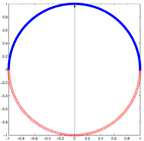
Figure 1: [Color online] An infinite LHS ensemble on the equator of the Bloch sphere. If the measurement axis is in the direction of the black vector, then Alice would report results $-1$ or $+1$ depending on whether the state she has sent in the aligned (blue solid circles) or antialigned (red circles) subensemble.

IV.2 Nonlinear EPR-steering inequality

As discussed in Ref. CavEtalPRA09 , nonlinear EPR-steering inequalities are in general better able to detect experimental steerability than simple linear inequalities. As we will show, that is the case here. In order to derive the inequality we make use of the linear inequality of the previous section involving equatorial observables, and augment it with a single additional non-equatorial Bob-observable, $\hat{\sigma}_{z}$. Once again, this involves no more extra work on Bob’s behalf, if he is already making a set of tomographically complete measurements, such as homodyne measurements BabEtalPRL04 . For Alice, it is in her best interests now to make a different measurement, $\hat{A}_{z}$, whenever Bob tells her that in this run he is interested in $\hat{\sigma}_{z}$. For simplicity we assume that $\hat{A}_{z}$ also has two possible outcomes: $a_{z}\in\{-1,1\}$. We show below, however, that even if Alice makes no measurement in this case, and merely always reports $a_{z}=+1$ (for instance), the inequality we derive is still stronger in general than the preceding one, Eq. (28).

Consider the following function

$$f(\{\langle\hat{\sigma}_{\theta}\rangle\},\langle\hat{\sigma}_{z}\rangle)=\frac{1}{\pi}\int_{-\pi/2}^{\pi/2}d\theta a_{\theta}\langle\hat{\sigma}_{\theta}\rangle-\frac{2}{\pi}\sqrt{1-\langle\hat{\sigma}_{z}\rangle^{2}},$$ (29)

which, as shown in Appendix VIII, is a convex function of its arguments and satisfies $f\leq 0\ \forall\ a_{\theta}\in\{-1,1\},\forall\ \rho$. Therefore, the constraint $f(\{\langle\hat{\sigma}_{\theta}\rangle\},\langle\hat{\sigma}_{z}\rangle)\leq 0$ defines an additive convex constraint on Bob’s system and using the approach of Sec. III.2 leads to the nonlinear EPR-steering inequality

$$\frac{1}{\pi}\int_{-\pi/2}^{\pi/2}d\theta E_{A_{\theta}}[a_{\theta}\langle\hat{\sigma}_{\theta}\rangle_{a_{\theta}}]-\frac{2}{\pi}E_{A_{z}}\left[{\sqrt{1-(\langle\hat{\sigma}_{z}\rangle_{a_{z}})^{2}}}\right]\leq 0.$$ (30)

Here $A_{z}$ ($A_{\theta}$) denotes the measurement Alice performs (or, as far as Bob is concerned, purports to perform) when Bob reveals that he has measured $\hat{\sigma}_{z}$ ($\hat{\sigma}_{\theta}$). Noting that the first term is the same as Eq. (27), and rearranging the inequality gives

$$\frac{1}{\pi}\int_{-\pi/2}^{\pi/2}d\theta\langle\hat{A_{\theta}}\hat{\sigma}_{\theta}\rangle\leq\frac{2}{\pi}E_{A_{z}}\left[{\sqrt{1-\langle\hat{\sigma}_{z}\rangle_{a_{z}}^{2}}}\right].$$ (31)

Finally, using our assumption that Alice’s observable $\hat{A}_{z}$ is dichotomic, we can write out the conditional expectation on the right hand side explicitly to obtain the nonlinear EPR-steering inequality

$$\frac{1}{\pi}\int_{-\pi/2}^{\pi/2}d\theta\langle\hat{A_{\theta}}\hat{\sigma}_{\theta}\rangle\leq\frac{2}{\pi}\left[\wp_{+}\sqrt{1-z_{+}^{2}}+\wp_{-}\sqrt{1-z_{-}^{2}}\right],$$ (32)

where $\wp_{\pm}$ is the probability that Alice obtains results $\pm 1$ and $z_{\pm}=\langle{\hat{\sigma}_{z}}\rangle_{\pm}$ are Bob’s respective conditional expectation values.

In general, the nonlinear bracketed term on the right hand side of Eq. (32) will be less than 1 and hence this side of the inequality will be less than $2/\pi$. Thus, as expected, the nonlinear EPR-steering inequality which incorporates an additional measurement setting, will be generally easier to violate than Eq. (28). Note that even if Alice’s observable is trivial ($\hat{A}_{z}=\hat{1}$), so that there is only one “result” ($\wp_{+}=1$) we obtain

$$\frac{1}{\pi}\int_{-\pi/2}^{\pi/2}d\theta\langle\hat{A_{\theta}}\hat{\sigma}_{\theta}\rangle\leq\frac{2}{\pi}\sqrt{1-\mathrm{Tr}\left[{{\hat{\sigma}_{z}\rho}}\right]^{2}},$$ (33)

where $\rho$ is Bob’s unconditioned reduced state. The right hand side here is still less than that of Eq. (28), except in the case that $\mathrm{Tr}\left[{{\hat{\sigma}_{z}\rho}}\right]=0$. This is the only case where Eq. (32) is not stronger than Eq. (28).

This example is similar to the so-called ‘inept state’ example of Ref. JonEtalPRA05 which suggests the following LHS model to model the correlations considered here. Consider two rings of pure states on the Bloch sphere centered around the $z$ axis, at $z=z_{-}$ and $z=z_{+}$. The ensemble is weighted so that it is invariant under rotations around the $z$-axis, and that so that the weighting of the upper (lower) ring is given by $\wp_{+}$ ($\wp_{-}$). By construction, such an ensemble will produce the correct correlations when Bob measures $\hat{\sigma}_{z}$, if Alice announces $a_{z}=+1$ ($a_{z}=-1$) when the LHS state she has sent is in the upper (lower) ring. Thus, we simply need to determine how well such an ensemble simulates correlations of the form $\langle\hat{A_{\theta}}\hat{\sigma}_{\theta}\rangle$. A straightforward calculation shows that the radii of the rings of pure states are given by $(1-z_{\pm}^{2})^{1/2}$. Taking the average over half of each ring centered around the measurement axis of interest results in the integral of Eq. (28), multiplied by each ring’s radius. Taking the weighted average, this LHS model can simulate a value for the left hand side of Eq. (32) equal to

$$\frac{2}{\pi}\left(\wp_{+}\sqrt{1-z_{+}^{2}}+\wp_{-}\sqrt{1-z_{-}^{2}}\right).$$ (34)

This proves that this ensemble of LHSs is optimal for these observables, and hence that Eq. (32) is a tight inequality.

IV.3 Finite setting inequality

The inequalities derived in the previous subsections assume that Alice can make an infinite number of measurements: a different $\hat{A}_{\theta}$ for each value of $\theta$ tested by Bob. In practice, a realistic experiment will be constrained to some finite number of measurement settings, such as a finite set of $\theta$ values. One might expect that using a finite number of settings will make it more difficult to demonstrate EPR-steering. While this is indeed the case, we show that we can modify Eq. (32) to account for this, and that the increase in difficulty is small even for moderate values of $n$.

Consider the case analogous to Sec. IV.1 but with $n$ evenly spaced equatorial measurements, which implies that the $\{\theta_{i}\}$ are separated by $\pi/n$. Assuming a LHS model for Bob’s subsystem ensures

$$\langle\hat{S}_{\rm plane}^{(n)}\rangle=\frac{1}{n}\sum_{i=1}^{(n)}\alpha_{i}\langle\hat{\sigma}_{\theta_{i}}\rangle\leq f(n),$$ (35)

where the bound is a function of the number of measurement axes and is given by

$$f(n)={}^{\rm max}_{\{\alpha_{i}\}}\lambda_{\rm max}(\hat{S}_{\rm plane}^{(n)}).$$ (36)

Following the approach used in the examples of Ref. SauEtalNat10 , one finds that the eigenvectors associated with the maximum eigenvalues obtainable for $\hat{S}_{\rm plane}^{(n)}$ occur along the direction of the measurement axes and a direction midway between measurement axes for $n$ odd and even respectively. Calculating these eigenvalues for the first few small $n$ allows one to obtain by induction

$$f(n)=\frac{1}{n}\left(\left|\sin\left(\frac{n\pi}{2}\right)\right|+2\sum_{k=1}^{\lfloor n/2\rfloor}\sin\left[\left(2k-1\right)\frac{\pi}{2n}\right]\right).$$ (37)

Proceeding analogously to Sec. IV.1, the constraint Eq. (35) results in the EPR-steering inequality

$$\frac{1}{n}\sum_{i=1}^{n}\langle\hat{A}_{i}\hat{\sigma}_{\theta_{i}}\rangle\leq f(n).$$ (38)

We can also incorporate an additional measurement axis orthogonal to the $n$ equatorial measurements, analogously to the proof in Sec. IV.2. We find that Eq. (32) is modified to

$$\frac{1}{n}\sum_{i=1}^{n}\langle\hat{A}_{i}\hat{\sigma}_{\theta_{i}}\rangle\leq f(n)\left[\wp_{+}\sqrt{1-z_{+}^{2}}+\wp_{-}\sqrt{1-z_{-}^{2}}\right].$$ (39)

Also following the method of Sec. IV.2 it is easy to see that the a two-ring LHS construction is optimal, but now with each ring containing a finite number of evenly space pure states. It follows on average the finite ensembles will predict

$$\frac{1}{n}\sum_{i=1}^{n}\langle\hat{A}_{i}\hat{\sigma}_{\theta_{i}}\rangle=g(n)\left[\wp_{+}\sqrt{1-z_{+}^{2}}+\wp_{-}\sqrt{1-z_{-}^{2}}\right],$$ (40)

To prove that Eq. (39) is tight it remains for us to prove that the functions $g(n)$ are the same as the $f(n)$ of Eq. (37) for the optimal arrangement for the pure states in the LHS ensemble.

Consider the first few even and odd examples for $n$ as shown in Fig. 2 (in the diagram a single ring is shown, but the optimal arrangement of LHSs will be the same for both rings). For the first even cases, $n=2$ and $n=4$, the ensembles that minimize $g(n)$ have pure states lying midway between the measurement axes (this reflects the directions of the maximum eigenvectors of $\hat{S}^{(2)}$ and $\hat{S}^{(4)}$). For the first odd cases, $n=3$ and $n=5$, the optimal ensembles have pure states aligned with the measurement axes (reflecting the directions of the maximum eigenvectors of $\hat{S}^{(3)}$ and $\hat{S}^{(5)}$). Partitioning each of these ensembles in half (as indicated in Fig. 2) leads to $g(2)=1/\sqrt{2}$, $g(3)=2/3$, $g(4)\approx 0.6533$, and $g(5)\approx 0.6472$. It is straightforward to show that these results generalise as one would expect for larger $n$ (with ensembles of $2n$ pure states off-axis per ring for even $n$, and $2n$ pure states on-axis per ring for odd $n$). Moreover, $g(n)=f(n)$ for all $n$. Thus, Eq. (40) saturates the right hand side of Eq. (39) and so the latter is indeed a tight EPR-steering inequality.

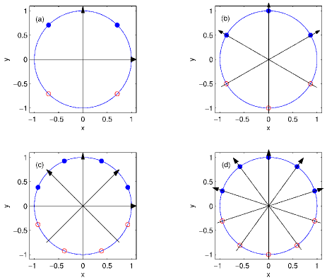
Figure 2: [Color online] Finite LHS ensembles around a circular plane. In each case the black vectors denote $n$ measurement axes, and the coloured dots denote pure states. Plots (a) and (c) correspond to the first two even cases, $n=2$ and $n=4$ respectively and have optimal ensembles of states lying midway between the measurement axes. Plots (b) and (d) correspond to the first two odd cases, $n=3$ and $n=5$ respectively and have optimal ensembles aligned with the measurements axes. In each case the blue (solid) and red colouring of the pure states denotes the partitioning of the ensemble that Alice would use if the $y$-axis was the measurement of interest for a particular run of an experiment.

It can be seen in Fig. 3 that the function $f(n)$ quickly approaches its asymptotic value. Hence, it takes relatively few equatorial measurement settings to arrive at an EPR-steerability criterion which works almost as well as the ideal criterion which incorporates an infinite number of measurement settings. Note that in the limit $n\rightarrow\infty$, $f(\infty)\to 2/\pi$ and Eq. (39) is equivalent to Eq. (32).

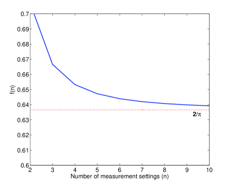
Figure 3: The finite correction factor $f(n)$ for some small values of the number of equatorial measurements used, $n$. We see that $f(n)$ quickly approaches the asymptotic value of $2/\pi$ (indicated by the red dotted line).

V EPR-steering of a single photon

V.1 Evenly split single photon state

We will now apply the EPR-steering inequalities derived in the preceding section to the single-photon state introduced in Sec. II.1, with Alice’s measurements constrained (as in experiment) to homodyne detection as introduced in Sec. II.2, supplemented by photon counting as introduced in Sec. II.3. We begin by considering the case where $\chi=0.5$, that is, when the intended initial state $W_{\eta}^{\chi}$ is maximally entangled in the limit $\eta\to 1$.

Consider the most general case using the nonlinear EPR-steering inequality defined in Eq. (39), as this allows for both homodyne ($A_{\theta}$) and photodetection ($A_{z}$) measurements. We must take into account the homodyne measurement inefficiency when evaluating the left hand side of the inequality; the photodetection inefficiency will manifest in the right hand side of the inequality.

Thus we wish to calculate the maximum value of $\frac{1}{\pi}\int_{0}^{\pi}d\theta\langle\hat{A_{\theta}}\hat{\sigma}_{\theta}\rangle$ allowed by quantum theory, given that Alice is restricted to homodyne measurements. However, this may be simplified by noting that in the state $W_{\eta}^{\chi}$, for every angle $\theta$ the maximum value of the correlation will be obtained when Alice chooses the phase of the local oscillator to be $\theta$, and reports a result $a_{\theta}=a(r)$, where $a(r)$ is negatively related to her homodyne measurement result $r$. This will result in the same value for the correlation function for every direction. Hence the correlation function becomes independent of $\theta$ and we have

$$\frac{1}{\pi}\int_{-\pi/2}^{\pi/2}d\theta\langle\hat{A}_{\theta}\hat{\sigma}_{\theta}\rangle=\max_{a(r)}\left(\int dr{\rm Tr}[\tilde{\rho}_{B}^{0}(r)\hat{\sigma}_{x}a(r)]\right),$$ (41)

where $\tilde{\rho}_{B}^{0}(r)$ is Bob’s conditioned state defined in Eq. (8), evaluated for $\theta=0$, and the function $a(r)$ is Alice’s reported result. Recall that in deriving the ineqality (39) we assumed that $a(r)\in\{-1,1\}$, but apart from that restriction, Alice is free to report any function of her result $r$. Using Eq. (8), Eq. (41) evaluates to

$$\max_{a(r)}\left(-\eta\sqrt{\eta_{\rm h}}\int_{-\infty}^{\infty}dr\frac{r}{\sqrt{2\pi}}\exp(-r^{2}/2)a(r)\right).$$ (42)

The maximum over $a(r)$ occurs when Alice chooses $a(r)=-{\rm sign}(r)$ and thus we have

$$\frac{1}{\pi}\int_{0}^{\pi}d\theta\langle\hat{A_{\theta}}\hat{\sigma}_{\theta}\rangle = \sqrt{\frac{2}{\pi}}\,\eta\sqrt{\eta_{\rm h}}.$$ (43)

Recall that $\eta$ is the efficiency of production of the single photon, while $\eta_{\rm h}$ is the efficiency of Alice’s homodyne measurement. It is easy to verify that exactly the same equation holds when the left-hand-side of Eq. (43) is replaced by a finite sum, as in the left-hand-side of Eq. (39).

Now we evaluate the right hand side of Eq. (39) for the case when Alice conditions using inefficient photodetection. The quantities in the right hand side of Eq. (39) were already determined in Sec. II.3. Substituting these in with $\chi=1/2$, we find that Eq. (39) will be violated iff

$$\sqrt{\frac{2}{\pi}}\,\eta\sqrt{\eta_{\rm h}}>f(n)\sqrt{\eta(2-\eta-\eta\eta_{\rm p})}.$$ (44)

In the limit $n\to\infty$, this can be rearranged to give the simple inequality

$$\eta>\frac{4}{2+\pi\eta_{\rm h}+2\eta_{\rm p}}.$$ (45)

This is a sufficient condition on the three parameters ($\eta,\eta_{\rm h},\eta_{\rm p}$) for experimental demonstration of EPR-steering. It may be visualized by a contour plot as shown in Fig. 4. The contours show the required minimum value of $\eta$, as a function of $\eta_{\rm h}$ and $\eta_{\rm p}$. Note that for low measurement efficiencies no contours are plotted as the preparation efficiencies required according to Eq. (45) would be unphysical ($\eta>1$). Note also that even without photodetection ($\eta_{\rm p}=0$), it would be possible (in principle) to satisfy this sufficient condition provided $\eta_{\rm h}$ and $\eta$ are high enough. But with $\eta_{\rm h}=0$ the inequality can never be satisfied, and this is because it is impossible for Alice to demonstrate EPR-steering with a single measurement.

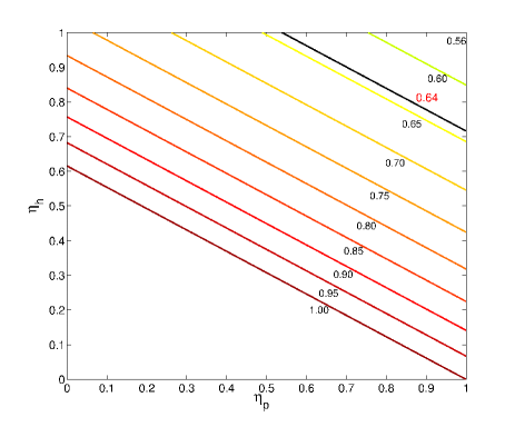
Figure 4: The pale contours indicate the value of $\eta$ required to demonstrate steering with inefficient homodyne and photodetection measurements. For lower measurement efficiencies there are no contours, as it would require unphysical values of $\eta$ (i.e. $\eta>1$) to satisfy the steerability criterion. The black contour ($\eta=0.64$) marks the preparation efficiency limit achieved experimentally in BabEtalPRL04 .

V.2 Unevenly split single photon state

The above analysis generalizes easily to the case of an unevenly split photon $W_{\eta}^{\chi}$, where $\chi$ can take any value between 0 and 1. The specific cases reported in BabBreLvoPRL04 were $\chi=0.5$ and $\chi=0.92$. We predict that the EPR-steering inequality Eq. (39) can be violated if

$$2\sqrt{\frac{2}{\pi}}\eta\sqrt{\eta_{\rm h}\chi(1-\chi)}>f(n)\sqrt{4\eta\chi\left[1-\eta\chi-\eta\eta_{\rm p}(1-\chi)\right]}.$$ (46)

Retaining this time a fully general result by not taking the number of Alice’s homodyne settings to infinity, we find the following sufficient condition:

$$\eta\left[\chi+(1-\chi)\left(\eta_{\rm p}+\frac{2}{\pi}\frac{\eta_{\rm h}}{[f(n)]^{2}}\right)\right]>1.$$ (47)

In Sec. VII we give examples showing when Eq. (47) with finite settings could be satisfied in a real experiment.

VI Necessary condition for EPR-steering

While the sufficient condition of Eq. (47) is a useful guide to experiments, failure to satisfy this condition (in the limit $n\to\infty$) does not mean that it would be impossible to demonstrate EPR-steering with the state $W_{\eta}^{\chi}$ using homodyne detection (with arbitrary phase) and photon counting, with efficiencies $\eta_{\rm h}$ and $\eta_{\rm p}$ respectively. This is because there may exist a better EPR-steering inequality than the one (39) we have derived — that is, an inequality that can be violated in a larger region of parameter space. Perhaps surprisingly, however, we can derive a necessary condition on the experimental parameters $\chi$, $\eta$, $\eta_{\rm h}$ and $\eta_{\rm p}$ for EPR-steering to be demonstrated, that makes no assumption on the inequality to be tested.

First, we consider the basic fact that in order for EPR-steering to take place, Alice must be able to perform at least two distinct measurements. In an experimental setup, if an imperfectly prepared (with efficiency $\eta$) single photon is mixed with the vacuum at a $\chi:(1-\chi)$ beam splitter, then we arrive at the situation where Alice and Bob share the state $W_{\eta}^{\chi}$. In such an experiment, Alice is assumed to receive on average a proportion $(1-\chi)\eta$ of the light from the initial single photon. We now consider what Alice could do with this light.

It is central to the definition of EPR-steering that Bob cannot trust Alice. Thus he should not simply believe her if she says that her photodetectors and homodyne photo-receivers have efficiency $\eta_{\rm p}$ and $\eta_{\rm h}$ respectively. It could be that she actually has perfect detectors. Let us assume that to be the case. It follows that if the following inequality

$$(1-\chi)\eta\eta_{\rm p}+(1-\chi)\eta 2\eta_{\rm h}\leq(1-\chi)\eta,$$ (48)

is satisfied then, Alice could use a complicated scheme to partition her fraction of the light, and simultaneously perform photodetection and homodyne measurements of two orthogonal phases, with efficiencies $\eta_{\rm p}$, $\eta_{\rm h}$, and $\eta_{\rm h}$. This is demonstrated in Fig. 5 (for the case where the inequality is saturated), by showing the proportion of the original single photon which Alice is able to send to each of her (assumed perfect) detectors. Now homodyne measurements of two orthogonal phases with efficiency $\eta_{\rm h}$ enables Alice to simulate the result of a homodyne measurement at any phase $\theta$, by suitably combining the two results, with the same efficiency $\eta_{\rm h}$. Thus this setup allows Alice to perform all of her possible measurements in a single measurement (i.e. with no change of the apparatus). By definition however, a single measurement by Alice cannot demonstrate EPR-steering. Therefore, it is necessary that Eq. (48) be violated in order for EPR-steering to be possible.

Figure 5: If Eq. (48) is satisfied then it is possible that Alice could use the measurement scheme depicted here, which would not constitute EPR-steering. That is, providing she had arbitrarily good detectors, she could partition her fraction $(1-\chi)\eta$ of the light and use $\eta_{\rm p}$ of it for performing photodetection, and two portions of $\eta_{\rm h}$ to perform homodyne measurements of orthogonal quadratures. This is essentially a single, though complicated, measurement scheme which cannot demonstrate EPR-steering.

It is obvious that Eq. (48) reduces to the much simpler condition $\eta_{p}+2\eta_{h}\leq 1$. We write the condition as in Eq. (48) to more easily relate conceptually to the next inequality we derive, which is not as straightforward, and which is a stronger inequality. Recall that a non-trusting Bob is the concept at the heart of the definition of EPR-steering. Such a Bob would know that a clever Alice could obtain a larger fraction of the light from the initial single photon than the $(1-\chi)\eta$ shown in Fig. 5. Rather, a devious Alice may obtain access to the preparation of the initial single photon and recover the fraction $1-\eta$ of the light from this state that was thought to be lost in the inefficient preparation so that she receives a total fraction $1-\eta\chi$. In this case (and again assuming perfect detectors), Alice can simultaneously obtain results for all of her possible measurements, with the right efficiencies, by a complicated measurement on her ‘boosted’ fraction of the light, provided that

$$(1-\chi)\eta\eta_{\rm p}+(1-\chi)\eta 2\eta_{\rm h}\leq 1-\chi\eta.$$ (49)

This is demonstrated in Fig. 6, for the case where the inequality is saturated and Alice must use every bit of light available. Thus, in order for it to be possible for Bob to be convinced that Alice is not simply performing a complicated single measurement on her fraction of the light, the inequality (49) must be violated.

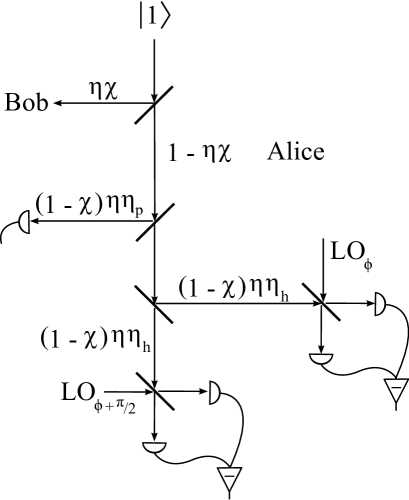
Figure 6: The setup is the same as in Fig. 5 however now Bob does not trust the initial preparation of the shared state. He knows that on average he receives $\eta\chi$ of the single photon, but he now assumes that Alice has access to the remaining $1-\eta\chi$ of the initial state, as well as having arbitrarily good detectors. In this case, she could again use a complicated measurement scheme to partition her fraction of the initial state to simultaneously perform both photodetection and homodyne measurements of orthogonal phases with efficiencies $\eta_{p}$ and $\eta_{h}$ respectively provided that Eq. (49) is satisfied.

Rearranging Eq. (49), we arrive at a necessary condition for it to be possible to demonstrate EPR-steering using the split-photon states $W_{\eta}^{\chi}$ and homodyne detection and photon counting:

$$\eta\left[\chi+(1-\chi)\left({\eta_{\rm p}+2\eta_{\rm h}}\right)\right]>1.$$ (50)

Note the similarity in form to the sufficient condition (47), and note that the necessary condition is strictly weaker than the sufficient condition.

VII Comparison with experiment

VII.1 Necessary conditions

Finally, we are in a position to reconsider the experiments BabBreLvoPRL04 ; BabEtalPRL04 . In the latter, Lvovsky and co-workers obtained experimental parameters of $\eta=0.64$, and $\eta_{\rm h}=0.86$, and in the former they used $\chi=0.5$ and $\chi=0.92$. First let us test these parameters in Eq. (50) to determine if EPR-steering was possible in this experiment. Evaluating the left hand side of the inequality we obtain $0.87$ and $0.68$ for $\chi=0.5$ and $0.92$ respectively. Clearly the necessary condition for steerability is not satisfied under either of these circumstances. Even if we add photodetection, with an efficiency $\eta_{\rm p}=0.3$ (which is experimentally feasible AltEtalOE05 ), we only raise these figures to $0.97$ and $0.69$ respectively, still short of the required value of $1$.

The easiest parameter to alter to try to improve the performance of the experiment is the splitting ratio $\chi$. As stated, the experiment of BabBreLvoPRL04 made use of a symmetric as well as a decidedly asymmetric arrangement (with Bob obtaining a much larger fraction of the light). In order to facilitate the demonstration of EPR-steering, we thus determine the optimal $\chi$. In the example above, the symmetric arrangement came much closer to satisfying the necessary condition than the asymmetric one. This might tempt one to conclude that the symmetric situation is most useful for a demonstration of EPR-steering. In fact, this is true neither for the necessary nor the sufficient criteria for EPR-steering.

Considering both Eq. (47) and Eq. (50) it is straightforward to see that $\chi=0$ is the optimal value for satisfying these conditions. However, physically this corresponds to the asymmetric case of Alice obtaining all of the light, in which case Alice and Bob do not share an entangled state at all and EPR-steering cannot occur. Thus, in practise the optimal arrangement would be to choose $\chi\ll 1$. (Experimental imperfections not modelled in our theory would presumably imply an optimal, small, value for $\chi$.) That is, in the Babichev et al. experiment BabBreLvoPRL04 , the asymmetry was weighted in the wrong direction — they had $\chi=0.92$, which sends almost all of the light to Bob.

We can understand this result intuitively, as it is Alice’s detection efficiencies that matter in the experiment, not Bob’s. Providing Alice with less of the initial state makes it more difficult for her to influence (steer) Bob’s part of the state. If the setup used in BabBreLvoPRL04 were to be reversed so that $\chi=0.08$, then with $\eta=0.64$, $\eta_{\rm h}=0.86$, and no photodetection ($\eta_{\rm p}=0$), the left hand side of Eq. (50) evaluates to $1.06$, suggesting that EPR-steering might be possible in an experiment similar to that in Ref. BabBreLvoPRL04 . Including photodection with $\eta_{\rm p}=0.3$, gives a left hand side of $1.24$, suggesting that EPR-steering should be possible using such an enhanced experiment.

VII.2 Sufficient conditions

In order to determine if these hypothetical experiments could demonstrate EPR-steering using the inequalities we have derived, we need to test the sufficient condition Eq. (47). We use the parameters of BabEtalPRL04 as above, with $\chi=0.08$ and we assume eight homodyne measurement settings. Using eight settings is few enough to seem experimentally feasible, but a large enough number so that $f(8)\simeq 0.641$ is not far from $f(\infty)=2/\pi\simeq 0.637$.

With no photodetection, the left hand side of the sufficient condition (47) evaluates to $0.84$. That is, unfortunately, the EPR-steering inequality we derived would be a long way from being violated. But including photodection with $\eta_{\rm p}=0.3$, gives a left hand side of $1.01$, implying that it would just be possible to violate Eq. (39), and so demonstrate EPR-steering, in this enhanced experiment.

In practice of course it would be extremely difficult for experimentalists to satisfactorily observe a violation which equates to $1.01>1.00$. Thus, in order to conclusively demonstrate EPR-steering of a single photon it would be desirable to have a larger violation of the steering criterion. The appeal of our approach is that we have provided a number of experimental parameters that may be adjusted to facilitate EPR-steering.

Consider first the case where there is no photodetection, as in the original experiments. Then if one chose $\chi=0.05$, and if one were able to improve the parameters to $\eta=0.78$ and $\eta_{\rm h}=0.92$, the sufficient condition (47) would be satisfied as follows: $1.10>1$. Alternatively, with photodetection included with efficiency $\eta_{\rm p}=0.30$, and with $\eta=0.66$ and $\eta_{\rm h}=0.90$, one would also find the same degree of violation. If one had access to a more efficient single-photon detector, the requirements on $\eta$ and $\eta_{\rm h}$ set by Eq. (47) become even less stringent. Thus demonstrating a substantial violation of an EPR-steering inequality with a single photon could be achieved with only moderate improvements to experimental techniques.

VIII Summary

In this work we have considered in detail the experimental prospects for demonstrating quantum nonlocality with a single photon, using homodyne detection. This question is of considerable interest experimentally, with both Bell-nonlocality (violation of a CHSH-inequality, with post-selection) BabEtalPRL04 , and “remote state preparation” (i.e. the EPR-steering phenomenon) BabBreLvoPRL04 of a single photon being addressed. Our analysis here shows that while the impure state produced in these experiments could not possibly be used to demonstrate violation of a CHSH-inequality without post-selection, it could be used to demonstrate EPR-steering, according to the definition established in Refs. WisEtalPRL07 ; JonWisDohPRA07 , without post-selection. Also, we showed that even given the efficiency of the homodyne detection used in these experiments, it might still be possible to do a rigorous demonstration of EPR-steering, if the asymmetry of the photon splitting were reversed from that used in Ref. BabBreLvoPRL04 .

To actually demonstrate EPR-steering would require violating an EPR-steering inequality, as defined in Ref. CavEtalPRA09 . Here we have introduced a family of such inequalities for homodyne detection on a single split photon, with an arbitrary number of different phase settings. Unfortunately with the experimental efficiency of homodyne detection achieved in Ref. BabEtalPRL04 , it would not be possible to violate any of these inequalities. However, we also generalized our inequality by supplementing homodyne detection with a photon detector. We showed that with a realistic photon detector efficiency, with relatively few different homodyne phases, and with only modest improvements to the efficiency of photon preparation and homodyne detection, it should be possible to achieve a substantial violation of our inequality. Thus, for rigorously demonstrating nonlocality (in the EPR-steering sense) of a single photon, in an experiment in the near future, the prospects are good.

Appendix A Convexity proof

We consider the function:

$$f(\{\langle\hat{\sigma}_{\theta}\rangle\},\langle\hat{\sigma}_{z}\rangle)=\frac{1}{\pi}\int_{-\pi/2}^{\pi/2}d\theta a_{\theta}\langle\hat{\sigma}_{\theta}\rangle-\frac{2}{\pi}\sqrt{1-\langle\hat{\sigma}_{z}\rangle^{2}},$$ (51)

with the aim of showing that

1. $f$ is a convex function of its arguments,

2. and that $f\leq 0$ $\forall\ a_{\theta}\in\{-1,1\},\forall\rho$.

In order to prove point 1, we must show that both terms in Eq. (51) are convex functions, as the sum of two convex functions is also a convex function RocCA70 . The first term is trivially convex, as the integral is just the continuous limit of adding the arguments, which are linear, and hence convex. For the second term, we need simply examine a plot of $-\sqrt{1-z^{2}}$ for $z\in\{-1,1\}$ to verify that it has a convex (i.e. concave up) shape.

Now to prove point 2, we must show that $f\leq 0$, $\forall\ a_{\theta}\in\{-1,1\},\forall\rho$. This amounts to showing that

$$\frac{1}{\pi}\int_{-\pi/2}^{\pi/2}d\theta a_{\theta}\langle\hat{\sigma}_{\theta}\rangle\leq\frac{2}{\pi}\sqrt{1-\langle\hat{\sigma}_{z}\rangle^{2}}.$$ (52)

It was shown in Sec. IV.1, that the maximum of the left hand side is occurs when $a_{\theta}\equiv 1$. Making this substitution and evaluating the integral means that we are required to prove the condition

$$\frac{2}{\pi}\langle\hat{\sigma}_{x}\rangle\leq\frac{2}{\pi}\sqrt{1-\langle\hat{\sigma}_{z}\rangle^{2}}.$$ (53)

That this holds for all $\rho$ follows immediately from the condition that $\langle\hat{\sigma}_{x}\rangle^{2}+\langle\hat{\sigma}_{z}\rangle^{2}\leq 1$.

References

- (1) S. M. Tan, D. F. Walls, and M. J. Collett, Phys. Rev. Lett. 66, 252 (1991).
- (2) L. Hardy, Phys. Rev. Lett. 73, 2279 (1994).
- (3) H. M. Wiseman and J. A. Vaccaro, Phys. Rev. Lett. 91, 097902 (2003).
- (4) S. J. van Enk, Phys. Rev. A 71, 032339 (2005).
- (5) J. Dunningham and V. Vedral, Phys. Rev. Lett. 99, 180404 (2007).
- (6) H. W. Lee and J. Kim, Phys. Rev. A 63, 012305 (2000).
- (7) E. Lombardi, F. Sciarrino, S. Popescu, and F. DeMartini, Phys. Rev. Lett. 88, 070402 (2002).
- (8) S. A. Babichev, J. Ries, and A. I. Lvovsky, Europhys. Lett. 64, 1 (2003).
- (9) S. A. Babichev, B. Brezger, and A. I. Lvovsky, Phys. Rev. Lett. 92, 047903 (2004).
- (10) S. A. Babichev, J. Appel, and A. I. Lvovsky, Phys. Rev. Lett. 92, 193601 (2004).
- (11) B. Hessmo, P. Usachev, H. Heydari, and G. Björk, Phys. Rev. Lett. 92, 180401 (2004).
- (12) S. D. Bartlett and H. M. Wiseman, Phys. Rev. Lett. 91, 097903 (2003).
- (13) S. J. Jones et al., Phys. Rev. A 74, 062313 (2006).
- (14) A. Einstein, B. Podolsky, and N. Rosen, Phys. Rev. 47, 777 (1935).
- (15) E. Schrödinger, Proc. Camb. Phil. Soc. 31, 553 (1935).
- (16) M. D. Reid, Phys. Rev. A 40, 913 (1989).
- (17) H. M. Wiseman, S. J. Jones, and A. C. Doherty, Phys. Rev. Lett. 98, 140402 (2007).
- (18) E. G. Cavalcanti, S. J. Jones, H. M. Wiseman, and M. D. Reid, Phys. Rev. A 80, 032112 (2009).
- (19) D. J. Saunders, S. J. Jones, H. M. Wiseman, and G. J. Pryde, Nature Physics 6, 845 (2010).
- (20) W. K. Wootters, Phys. Rev. Lett. 80, 2245 (1998).
- (21) R. Horodecki, P. Horodecki, and M. Horodecki, Phys. Lett. A 200, 340 (1995).
- (22) H. M. Wiseman, Quantum Semiclass. Opt. 7, 569 (1995).
- (23) H. M. Wiseman and R. B. Killip, Phys. Rev. A 56, 944 (1997).
- (24) K. A. Kirkpatrick, Found. Phys. Lett. 19, 95 (2006).
- (25) S. J. Jones, H. M. Wiseman, and A. C. Doherty, Phys. Rev. A 76, 052116 (2007).
- (26) M. D. Reid, P. D. Drummond, W. P. Bowen, and et al., Review of Modern Physics 81, 1727 (2009).
- (27) J. Oppenheim, Science 330, 1072 (2010).
- (28) S. J. Jones, H. M. Wiseman, and D. T. Pope, Phys. Rev. A 72, 022330 (2005).
- (29) J. B. Altepeter, E. R. Jeffrey, and P. G. Kwiat, Optics Express 13, 8951 (2005).
- (30) R. T. Rockafellar, Convex Analysis (Princeton Universiy Press, Princeton, NJ, 1970).