Abstract

We formulate a low energy effective theory describing phases of matter that are both solid and superfluid. These systems simultaneously break translational symmetry and the phase symmetry associated with particle number. The symmetries restrict the combinations of terms that can appear in the effective action and the lowest order terms featuring equal number of derivatives and Goldstone fields are completely specified by the thermodynamic free energy, or equivalently by the long-wavelength limit of static correlation functions in the ground state. We show that the underlying interaction between particles that constitute the lattice and the superfluid gives rise to entrainment, and mixing between the Goldstone modes. As a concrete example we discuss the low energy theory for the inner crust of a neutron star, where a lattice of ionized nuclei coexists with a neutron superfluid.

LA-UR-11-00458

1 Introduction

The low energy dynamics of strongly interacting solids and superfluids can be systematically studied through an effective theory formulation in terms of weakly interacting phonons - the collective degrees of freedom in these systems. In the familiar case of solids, one longitudinal phonon and two transverse phonons arise as Goldstone modes due to the breaking of translation symmetry. In the case of a superfluid, one mode called the superfluid phonon arises due to the breaking of the global $U(1)$ symmetry associated with phase rotations of a field operator . In special cases the ground state of the system can spontaneously break both these symmetries. A particularly simple but non-trivial realization is a solid immersed in a superfluid with strong interactions between the particles that form the solid and the superfluid respectively. It is likely that a substantial region in the crust of a neutron star is occupied by such a phase [1] and its presence may affect neutron star phenomenology. From general considerations we can argue that the inner crust of neutron stars features a lattice of neutron rich nuclei in a bath of unbound superfluid neutrons. The lattice sites can be viewed as clusters of protons, with a fraction of neutrons “entrained” on the clusters [2, 3]. Other intrinsically more complex phases where a single component exhibits both superfluid and solid characteristics have also been proposed. They include the supersolid phase of ⁴He [4] and the Larkin Ovchinnikov Fulde Ferrell (LOFF) phases [5, 6] in polarized fermion superfluids. Although these systems can in principle be realized terrestrially, they have proven to be challenging to explore in experiments [7]. Nonetheless in all these cases the low energy dynamics is described by an effective theory of four Goldstone modes [8]. The associated fields for the lattice phonons are $\xi^{a=1..3}({\bf{r}},t)$ and are related to space-time dependent deformations of the lattice. Similarly, the field associated with the superfluid mode $\phi({\bf{r}},t)$ is related to the space-time dependent phase of the condensate. Because of interactions, such as those between the neutrons and the protons in the neutron star crust, one can not in general treat the two sectors separately and a unified treatment is required. It is the aim of this paper to provide such a framework.

The low energy theory is described in terms of the fields $\phi$ and $\xi^{a}$. The symmetries associated with translation and number conservation require that the low energy theory be invariant under the transformation $\xi^{a=1..3}({\bf{r}},t)\rightarrow\xi^{a=1..3}({\bf{r}},t)+a^{a=1..3}$ and $\phi({\bf{r}},t)\rightarrow\phi({\bf{r}},t)+\theta$ where $a^{a=1..3}$ and $\theta$ are constant shifts. This naturally implies that the low energy lagrangian can contain only spatial and temporal gradients of these fields. Further, by requiring cubic symmetry for the crystalline state, the quadratic part of the effective lagrangian is given by,

$$\begin{split}{\cal{L}}=\frac{f_{\phi}^{2}}{2}&(\partial_{0}\phi)^{2}-\frac{v_{\phi}^{2}f_{\phi}^{2}}{2}(\partial_{i}\phi)^{2}+\frac{\rho}{2}\partial_{0}\xi^{a}\partial_{0}\xi^{a}-\frac{1}{4}{{\mu}}(\xi^{ab}\xi^{ab})-\frac{{K}}{2}(\partial_{a}\xi^{a})(\partial_{b}\xi^{b})\\ &-\frac{\alpha}{2}\sum_{a=1..3}(\partial_{a}\xi^{a}\partial_{a}\xi^{a})+{g_{\rm mix}f_{\phi}\sqrt{\rho}}~{}\partial_{0}\phi\partial_{a}\xi^{a}+\cdots~{}\;,\end{split}$$ (1)

where higher order terms involve higher powers of the gradients of these fields, and $\xi^{ab}=(\partial_{a}\xi^{b}+\partial_{b}\xi^{a})-\frac{2}{3}\partial_{c}\xi^{c}\delta^{ab}$. In the uncoupled case, the low energy coefficients (LECs) appearing above, such as $\rho,{\mu},{K}$ are related to the mass density, the shear modulus, and the compressibility of the solid respectively. They determine the velocities of the phonons in the solid phase. Similarly, the velocity of the phonon in the pure superfluid case is given by $v_{\phi}$. In the presence of strong coupling between the solid and superfluid these coefficients are modified. For example, the coefficient $\rho$ in Eq. 1 differs from the usual mass density of the pure lattice component due interactions that entrain the superfluid, and the mixing coefficient $g_{\rm mix}$ couples superfluid and lattice dynamics. As we will show Galilean invariance relates $g_{\rm mix}$ to the modifications of $\rho$ and $v_{\phi}$ due to entrainment [9]. An analysis of these modifications in the context of the neutron star crust due to the underlying interaction between neutrons and protons was the original motivation for this study. In this case, the mixing coefficient $g_{\rm mix}$ is relevant for heat transport properties in the inner crust [10], and the eigenmodes of the coupled superfluid-solid system could play a role in explaining the observed quasi-periodic oscillations in magnetars flares [11].

We will present a general proof that the functional form of the lowest-order Lagrangian is completely specified by the thermodynamic pressure in the presence of constant external fields that couple to the conserved densities and currents in the system. The derivatives of the pressure with respect to these external fields determine the low energy constants. Non-perturbative techniques such as Quantum Monte Carlo or Hartree-Fock techniques may be suited to calculate these thermodynamic functions. For example, the energy as a function of the density for a non-relativistic uniform Fermi gas at unitarity was calculated using Quantum Monte Carlo techniques in [12]. (For a recent example of the calculation of the LECs in relativistic superfluids, see [13].) Since these derivatives of the thermodynamic functions are related to the long-wavelength limit of static correlation functions of currents and densities, their direct calculation using non-perturbative methods also provide the needed LECs.

The outline of the paper is as follows. In Section 2 we outline the formalism and define notation. In Section 3 we revisit the effective theory of a neutron superfluid in the absence of any lattice, derived earlier in Ref. [14, 15]. This serves as a pedagogic warm-up before describing the more complicated system including the lattice. Here, we prove that lowest order lagrangian is determined by the thermodynamic pressure. In Section 4 we derive results for the relevant case of the combined neutron and proton sectors. In Section 5 we focus on the applications of our formalism to the neutron star crust and use simple estimates for the mixing coefficient in the neutron star inner crust to determine the resulting eigenmodes of the longitudinal lattice and the superfluid phonons. Here we also comment on the connection with previous work on the elastic properties of LOFF phases [16]. We present our conclusions in Section 6.

2 Symmetries of the underlying Hamiltonian  

The prototypical system we consider here is composed of two conserved species of particles. In the neutron stars, this would be the strongly coupled many-body system of non-relativistic neutrons and protons. In what follows we will continue to refer to these two components as neutron and protons but it should be understood that our considerations apply more generally. We represent the action for the system abstractly as ${\cal{S}}[\Psi_{n},\Psi_{p}]$ where $\Psi_{n}$ and $\Psi_{p}$, are the neutron and proton fields. Even though the particles may be non-relativistic, we will work in a Lorentz covariant form and take the non-relativistic limit at the end of the calculation. We will denote the spatial indices by Latin characters ($a$, $b$, $c$, $i$, $j$, $k$) running from $1$ to $3$ and the full space-time indices by Greek characters ($\mu$, $\nu$, $\sigma$, $\lambda$) running from $0$ to $3$.

The theory describing the neutrons and protons is invariant with respect to global phase rotations of the neutron field, $\Psi_{n}(x)\rightarrow\exp(-i\theta_{n})\Psi_{n}(x)$. The conservation law associated with the symmetry is the conservation of neutron number. Similarly, independent phase rotations of the protons gives rise to the conservation of proton number. We note that protons and neutrons are separately conserved on timescales small compared to the weak interaction time $\tau_{\rm weak}\simeq 1/(G_{F}^{2}~{}n_{B}~{}T^{2})$ where $n_{B}$ and $T$ are the baryon density and temperature of the system. For typical conditions the timescale for low energy dynamics is $\tau_{\rm EFT}\simeq 1/T$ and correspondingly the ratio $\tau_{\rm EFT}/\tau_{\rm weak}\simeq G_{F}^{2}n_{B}T\ll 1$. We shall refer to the corresponding conserved currents as $j^{\mu}_{n}$ and $j^{\mu}_{p}$ respectively. The action ${\cal{S}}$ is also invariant under space-time translations and spatial rotations and the conserved current associated with translations is the stress energy tensor $T^{\mu\nu}$.

To analyze the constraints provided by these symmetries on the low energy effective action, it is useful to introduce external fields that couple to the conserved currents (see e.g. discussion in Ref. [17]). For the internal symmetries we add to the action ${\cal{S}}[\Psi_{n},\Psi_{p}]$ source terms of the form $\int d^{4}x\;j^{\mu}_{n}(x)A_{\mu}^{n}(x)$ and $\int d^{4}x\;j^{\mu}_{p}(x)A_{\mu}^{p}(x)$. If the external fields are allowed to transform appropriately under local $U(1)$ transformations, this procedure promotes the global symmetries to local symmetries. This is equivalent to converting all partial derivatives $\partial_{\mu}$ to covariant derivatives $\partial_{\mu}-iA_{\mu}$.

A similar extension of space-time symmetries is slightly more subtle. It requires extending space-time from a flat space-time to a curved space-time, and writing the action in a form that is general coordinate invariant. Indeed, the non-relativistic theory of neutrons and protons may be seen as the non-relativistic, flat-space limit, of a fully relativistic, general-coordinate-invariant action. The external field that couples to the stress-energy tensor is a deformation of the metric, $\delta g_{\mu\nu}$.

Therefore, we start with an action of the form, ${\cal{S}}[\Psi_{n},\Psi_{p},A_{\mu}^{n},A_{\mu}^{p},g_{\mu\nu}]$ which is invariant under general coordinate transformations,

$$\begin{split}x^{\mu}&\rightarrow x^{{}^{\prime}\mu}=x^{\mu}+a^{\mu}(x)\\ g^{\mu\nu}(x)&\to g^{{}^{\prime}\mu\nu}(x^{\prime})=g^{\rho\sigma}(x)\frac{\partial x^{{}^{\prime}\mu}}{\partial x^{\rho}}\frac{\partial x^{{}^{\prime}\nu}}{\partial x^{\sigma}}\\ A^{\mu}(x)&\rightarrow A^{{}^{\prime}\mu}(x^{\prime})=A^{\sigma}(x)\frac{\partial x^{{}^{\prime}\mu}}{\partial x^{\sigma}}\;,\end{split}$$ (2)

these transformations include both rotations and boosts as special cases of local space and time translations. The action is also invariant under local phase rotations of neutrons,

$$\begin{split}\Psi_{n}(x)&\rightarrow\Psi_{n}^{\prime}(x)=\exp(-i\theta_{n}(x))\Psi_{n}(x)\\ A^{n}_{\mu}(x)&\rightarrow A^{{}^{\prime}n}_{\mu}(x)=A^{n}_{\mu}(x)-\partial_{\mu}\theta^{n}(x)\;,\end{split}$$ (3)

and local phase rotations of protons,

$$\begin{split}\Psi_{p}(x)&\rightarrow\Psi^{\prime}_{p}(x)=\exp(-i\theta^{p}(x))\Psi_{p}(x)\\ A^{p}_{\mu}(x)&\rightarrow A^{{}^{\prime}p}_{\mu}(x)=A^{p}_{\mu}(x)-\partial_{\mu}\theta^{p}(x)\;.\end{split}$$ (4)

The reason for extending the global symmetries to local symmetries is that correlation functions of the conserved currents can be analyzed very simply by taking appropriate functional derivatives of the generating functional $W[A_{\mu}^{n},A_{\mu}^{p},g_{\mu\nu}]$ with respect to the external fields $A_{\mu}^{n}(x),A_{\mu}^{p}(x)$ and $g_{\mu\nu}(x)$. The generating functional is defined in the standard path integral representation as

$$\begin{split}e^{iW[A_{\mu}^{n},A_{\mu}^{p},g_{\mu\nu}]}&=\int[d\Psi_{n}][d\Psi_{p}]e^{i{\cal S}[\Psi_{n},\Psi_{p},A_{\mu}^{n},A_{\mu}^{p},g_{\mu\nu}]}\\ &=Z[A_{\mu}^{n},A_{\nu}^{p},g_{\mu\nu}]\,;\end{split}$$ (5)

and $Z[A_{\mu}^{n},A_{\nu}^{p},g_{\mu\nu}]$ is thermodynamic partition function. For example, the derivative with respect to the zeroth component of the external field $A_{\mu}$ defines the number density as given by

$$\begin{split}\langle\Omega|\hat{n}_{n}(x)|\Omega\rangle_{A_{\mu}^{n},A_{\mu}^{p},g_{\mu\nu}}&=\frac{\delta W[A_{\mu}^{n},A_{\mu}^{p},g_{\mu\nu}]}{\delta A_{0}^{n}(x)}=\frac{1}{iZ}\frac{\delta Z[A_{\mu}^{n},A_{\mu}^{p},g_{\mu\nu}]}{\delta A^{n}_{0}(x)}~{}.\end{split}$$ (6)

In order to evaluate correlation functions in an equilibrium state with specified number density, the functional derivatives with respect to $A_{\mu}(x)$ are evaluated at specific values corresponding to appropriate chemical potentials as required by Eq. 6. For neutrons $A^{n}_{\mu}(x)={\bar{A}}^{n}_{\mu}=(\mu_{n}+m_{n},{\bf{0}})$, where $\mu_{n}$ is the usual non-relativistic chemical potential and similarly for protons $A^{p}_{\mu}(x)={\bar{A}}^{p}_{\mu}=(\mu_{p}+m_{p},{\bf{0}})$ and $\mu_{p}$ is the corresponding non-relativistic chemical potential. Moreover, functional derivatives with respect to $g_{\mu\nu}(x)$ are evaluated at space-time metric $g_{\mu\nu}(x)={\bar{g}}_{\mu\nu}$. For the pure neutron sector (Section 3), it suffices to set the equilibrium metric to be the Minkowski metric, ${\bar{g}}_{\mu\nu}=\eta_{\mu\nu}$. In the case of coupled system, since the spatial components of a space-time independent metric specifies the lattice structure, we will allow ${\bar{g}}_{\mu\nu}$ to be more general in Section 4. In the following we discuss specific cases in which the ground state $|\Omega\rangle$ spontaneously breaks number and translation symmetries of the underlying Hamiltonian. First, in Section 3 we discuss the simple case of a superfluid which breaks the $U(1)$ symmetry associated with number conservation, and subsequently in Section 4 we discuss the system of interest where both the global $U(1)$ and space-time translation symmetries are simultaneously broken.

3 One component superfluid 

3.1 Fields and the effective lagrangian

To illustrate the main ideas we first consider a single component superfluid such as degenerate neutron matter where attractive interactions lead to the formation of Cooper pairs and a transition to a superfluid state. Here, the two-neutron operator has a non-zero expectation value and in equilibrium

$$\langle\Omega|\Psi_{n}(x)\Psi_{n}^{T}(x)|\Omega\rangle=C\gamma^{5}\Theta(x)=C\gamma^{5}|\Theta|\;.$$ (7)

Since the phase of the condensate changes on making a global phase rotation on $\Psi_{n}$, the condensate spontaneously breaks $U(1)_{n}$ to $Z_{2}$. The corresponding Goldstone boson field $\phi(x)$ is given by the phase fluctuations of the order parameter.

The field $\phi(x)$ transforms nonlinearly under $U(1)_{n}$ transformations with parameter $\theta_{n}$:

$$\phi\to\phi+\theta_{n}~{}.$$ (8)

The effective Lagrangian for $\phi$ can be in principle obtained by integrating out the heavy modes corresponding to the gapped fermionic excitations from the system in a Wilsonian approach.

The partition function in presence of external gauge fields admits the following low-energy representation:

$$Z_{n}[A_{\mu}^{n},g_{\mu\nu}]=\int[d{\Psi}_{n}]e^{i{\cal S}[{\Psi}_{n},A_{\mu}^{n},g_{\mu\nu}]}\ \longrightarrow\ \int[d\phi]e^{i{\cal S}_{\rm eff}[\partial_{\mu}\phi,A_{\mu}^{n},g_{\mu\nu}]}\;.$$ (9)

The symmetries of the underlying fundamental theory impose stringent constraints on the form of the effective lagrangian defined by ${\cal S}_{\rm eff}=\int d^{4}x\sqrt{-g}\,{\cal{L}}_{\rm{eff}}$. Global $U(1)_{n}$ symmetry implies that the Goldstone boson can occur only through the derivative $\partial_{\mu}\phi$ and local $U(1)_{n}$ symmetry (Eq. 3) implies that $A_{\mu}^{n}$ and $\phi$ can appear in ${\cal{L}}_{\rm{eff}}$ only in the combination

$$D_{\mu}\phi(x)=\partial_{\mu}\phi(x)+A_{\mu}^{n}(x)\;.$$ (10)

Since we are working in a covariant theory, ${\cal{L}}_{{\rm{eff}}}$ should transform as a scalar density under general coordinate transformations. Therefore, the effective lagrangian can only be constructed from building blocks like $D_{\mu}\phi$, $D_{\nu}D_{\mu}\phi$ etc., with all indices contracted.

In this work we use the power counting scheme proposed by Son and Wingate [15] to organize terms in ${\cal{L}}_{{\rm{eff}}}$. We define the power of an operator as the difference between the number of $\partial$’s and the power of $\phi$. I.e. all terms of order $(\partial)^{m}(\phi)^{n}$ ($m\geq n$) with the same value of $m-n$ are considered to have the same order, $m-n$. $A_{\mu}^{n}$ has the same order as $\partial_{\mu}\phi$, i.e. order $0$, and $g_{\mu\nu}$ also has order $0$. Therefore,

$$\begin{split}{\cal{L}}_{{\rm{eff}}}[D_{\mu}\phi,g_{\mu\nu}]&={\cal{L}}_{0}[D^{\mu}\phi D_{\mu}\phi]+{\cal{L}}_{2}[(D^{\nu}D_{\mu}\phi)^{2},...]+...\end{split}$$ (11)

and the leading order lagrangian ${\cal L}_{0}$ is an arbitrary function of the building block $X=g^{\mu\nu}D_{\mu}\phi D_{\nu}\phi$. In what follows we will focus on the lowest order lagrangian and relate its coefficients to the thermodynamic derivatives.

3.2 Thermodynamic matching

We now relate the functional dependence of ${\cal L}_{0}(X)$ on $X$ to the functional dependence of the thermodynamic pressure $P(\mu_{n})$ on the chemical potential $\mu_{n}$. We refer to this result as to “thermodynamic matching”. Although this result is not new [14, 15], here we provide a derivation that can be generalized to other, more complex patterns of symmetry breaking. In fact, we will use the generalization of this result in Section 4 when we consider the simultaneous breaking of translational and particle-number symmetry.

We recall that the thermodynamic interpretation of the functionals $Z[A^{n}_{\mu},g_{\mu\nu}]$ and $W[A^{n}_{\mu},g_{\mu\nu}]$ at constant external fields ($A_{\mu}^{n}(x)={\bar{A}}_{\mu}^{n}$ and $g_{\mu\nu}(x)={\bar{g}}_{\mu\nu}=\eta_{\mu\nu}$) is given by the relation

$$\begin{split}Z_{n}[{\bar{A}}_{\mu}^{n},\eta_{\mu\nu}]&=e^{iW_{n}[{\bar{A}}_{\mu}^{n},\eta_{\mu\nu}]}=e^{-iVT\Omega_{n}}=\int[d\phi]\,e^{i{\cal S}_{\rm eff}[{\bar{D}}_{\mu}\phi,\eta_{\mu\nu}]}~{},\end{split}$$ (12)

where $\Omega_{n}=\langle\Omega|\hat{H}-{\bar{A}}^{n}_{\mu}j_{n}^{\mu}|\Omega\rangle$ is the free energy density, $V$ is the volume and $T$ is the extent in the time direction. Here $|\Omega\rangle$ is the ground state of the Hamiltonian modified by the presence of the external source $\bar{A}^{n}_{\mu}$ ($\hat{H}$ is the Hamiltonian density). For the specific choice $\bar{A}^{n}_{\mu}=(m_{n}+\mu_{n},\vec{0})$ and at zero temperature, $|\Omega\rangle$ is the many-body ground state at chemical potential $\mu_{n}$ and $\Omega_{n}=\langle\Omega|\hat{H}-(\mu_{n}+m_{n})\hat{j}^{0}_{n}|\Omega\rangle=-P(\mu_{n})$, where $P(\mu_{n})$ is the usual thermodynamic pressure of the system.

The low energy effective action ${\cal S}_{\rm eff}[{\bar{D}}_{\mu}\phi,\eta_{\mu\nu}]$ is a function of the external fields and the Goldstone fields. It contains all the quantum dynamics of the high energy Fermionic modes encoded as low energy coefficients. In order to evaluate the partition function $Z[A^{n}_{\mu},g_{\mu\nu}]$ we expand the effective action about its saddle point $\phi_{0}$ which satisfies

$$\frac{\delta{\cal S}_{\rm eff}[\bar{D}_{\mu}\phi(x),\eta_{\mu\nu}]}{\delta\phi(x)}|_{\phi_{0}}=0=-\partial_{\mu}\frac{d{\cal{L}}_{{\rm{eff}}}({\bar{D}}_{\mu}\phi(x),\eta_{\mu\nu})}{d\partial_{\mu}\phi(x)}|_{\phi_{0}}\;,$$ (13)

minimizes the Euclidean action, and is well behaved at infinity. For general external fields $A_{\mu}^{n}(x)$, the solution to Eq. 13 is a functional of the external field, $\phi_{0}[A_{\mu}^{n}]$. However, for our homogeneous and static system with constant external fields the well behaved solution is $\phi_{0}=0$. Expanding about this point we can write

$${\cal S}_{\rm eff}[{\bar{D}}_{\mu}\phi,\eta_{\mu\nu}]={\cal S}_{\rm eff}|_{\phi_{0}=0}+\frac{1}{2}\int d^{4}xd^{4}x^{\prime}\varphi(x)\varphi(x^{\prime})\frac{\delta^{2}\cal S_{\rm eff}}{\delta\phi(x)\delta\phi(x^{\prime})}|_{\phi_{0}}+...\;,$$ (14)

where $\varphi=\phi-\phi_{0}$, and thus Eq. 12 can be evaluated as a loop expansion

$$e^{iW[{\bar{A}}_{\mu}^{n},\eta_{\mu\nu}]} = e^{i{\cal S}_{\rm eff}|_{\phi_{0}=0}+W_{\rm 1-loop}+\cdots}$$ (15)

$$e^{iW_{\rm 1-loop}} = \int[d\varphi]e^{i(\frac{1}{2}\int d^{4}xd^{4}x^{\prime}\varphi(x)\varphi(x^{\prime})\frac{\delta^{2}{\cal{S}}_{\rm eff}}{\delta\phi(x)\delta\phi(x^{\prime})}|_{\phi_{0}}+...)}~{},$$ (16)

where we have explicitly displayed only the quadratic (Gaussian) part of the functional integral in $[d\varphi]$ which corresponds to the one-loop approximation. Let us now discuss this loop expansion in light of the EFT power counting. The key observation, which is a generic feature of low-energy effective theories [18], is the following: within the momentum (gradient) expansion of the EFT, loop diagrams generated by ${\cal{L}}_{0}$ are higher order than tree-level diagrams with vertices from ${\cal L}_{0}$. In our case, one-loop contributions to phonon amplitudes are suppressed by four powers of momenta compared to the tree graphs generated by ${\cal{L}}_{0}$ as shown by Son and Wingate [15]. Using the above considerations we can write

$$\begin{split}W[A_{\mu}^{n}]&=\int d^{4}x{\cal{L}}_{{\rm{eff}}}\bigl{(}(D_{\mu}\phi_{0}[A_{\mu}^{n}]),\eta_{\mu\nu}\bigr{)}+W_{\rm{1-loop}}(A_{\mu}^{n})+...\\ &=\int d^{4}x\,\Big{[}{\cal{L}}_{0}\bigl{(}X_{0}\bigr{)}+{\cal{L}}_{2}[A_{\mu}^{n}]+{\cal{L}}_{4}[A_{\mu}^{n}]\Big{]}+W_{\rm{1-loop}}(A_{\mu}^{n})+...~{},\end{split}$$ (17)

where $X_{0}=D_{\mu}\phi_{0}D^{\mu}\phi_{0}$. ${\cal{L}}_{0}\bigl{(}X_{0}\bigr{)}$ in Eq. 17 is the leading term (${\cal{O}}(p^{0})$), the second term is of ${\cal{O}}(p^{2})$, the third and fourth are ${\cal{O}}(p^{4})$. The contribution of ${\cal{O}}(p^{0})$ involves either no derivatives on the external fields or two derivatives compensated by a Goldstone propagator of ${\cal{O}}(p^{-2})$. Higher order contributions necessarily involve derivatives acting on the external field $A_{\mu}^{n}(x)$. So we arrive at a very important result: for very long wavelength external field ($A_{\mu}^{n}(x)\rightarrow{\rm{constant}})$, only the first term in Eq. 17 survives., i.e.,

$$W[{\bar{A}}_{\mu}^{n}]=\int d^{4}x\,{\cal{L}}_{0}({\bar{A}}_{\mu}^{n}{\bar{A}}^{\mu\;n})=VT\,{\cal{L}}_{0}({\bar{A}}_{\mu}^{n}{\bar{A}}^{\mu\;n})$$ (18)

Now recall that ${\bar{A}}_{\mu}{\bar{A}}^{\mu}=(m_{n}+\mu_{n})^{2}$ so that $\mu_{n}=\sqrt{{\bar{A}}_{\mu}{\bar{A}}^{\mu}}-m_{n}$. Moreover, ${\cal L}_{0}$ depends on $D_{\mu}\phi$ only through $X$. At the classical solution, for constant external field, one has $X\to X_{0}={\bar{A}}_{\mu}{\bar{A}}^{\mu}$. So we have from Eqs. 18 and 12,

$${\cal L}_{0}(X_{0})=P(\sqrt{{\bar{A}}_{\mu}{\bar{A}}^{\mu}}-m_{n})=P(\sqrt{X_{0}}-m_{n}=\mu_{n})~{}.$$ (19)

The above relation fixes the functional dependence of ${\cal L}_{0}$ on the variable $X$ once the functional dependence of $P$ on $\mu_{n}$ is known. So in general we have:

$${\cal L}_{0}(X)=P(Y\equiv\sqrt{X}-m_{n})~{}.$$ (20)

Finally we note that in the non-relativistic limit the relevant building block takes the form $Y=\sqrt{(m_{n}+\mu_{n}+\partial_{0}\phi)^{2}-(\partial_{i}\phi)^{2}}-m_{n}\ \simeq\mu_{n}+\partial_{0}\phi-\frac{(\partial_{i}\phi)^{2}}{2m_{n}}$ [14, 15, 19].

3.3 Identifying the low-energy constants

Eq. 20 gives us the complete expression of the superfluid lagrangian to the lowest order in $(m-n)$. Expanding the function ${\cal{L}}_{0}(\phi)$ in powers of the Goldstone fields, one can read off the phonon kinetic term and self-interaction vertices:

$$\begin{split}{\cal{L}}_{{\rm{eff}}}[\phi]&={\cal{L}}_{0}[(\mu_{n}+m_{n})^{2}]+\frac{dP}{dY}\,(\partial_{0}\phi)+\frac{1}{2!}\frac{d^{2}P}{dY^{2}}\,(\partial_{0}\phi)^{2}-\frac{1}{2!(\mu_{n}+m_{n})}\frac{\partial P}{\partial{Y}}\,(\partial_{i}\phi)(\partial_{i}\phi)\\ &+\frac{1}{3!}\frac{d^{3}P}{dY^{3}}\,(\partial_{0}\phi)^{3}+\frac{1}{2!}\left[-\frac{1}{(\mu_{n}+m_{n})}\frac{d^{2}P}{dY^{2}}+\frac{1}{(\mu_{n}+m_{n})^{2}}\frac{dP}{dY}\right](\partial_{0}\phi)(\partial_{i}\phi)(\partial_{i}\phi)+...~{}\end{split}$$ (21)

where all derivatives are evaluated at $Y=\mu_{n}$. The above expansion makes it clear that the low energy constants of the theory are then given by the derivatives of the pressure with respect to the chemical potential. Eq. 21 also serves as a starting point for a fluid dynamical study of the system once one realizes that $-\partial_{i}\phi/(m_{n}+\mu_{n})$ is the velocity of the superfluid. (See Ref. [20] and references therein.)

Alternatively, one can show that the thermodynamic derivatives are related to the static correlation functions involving the neutron charge and current operators. For example,

$$\frac{\partial W_{n}}{\partial{\bar{A}}_{\mu}^{n}}=\langle J_{n}^{\mu}(0)\rangle=\frac{dP}{dY}|_{eq}\eta^{\mu 0}\;.$$ (22)

Similarly,

$$\begin{split}\frac{\partial^{2}W_{n}}{\partial{\bar{A}}_{\nu}^{n}\partial{\bar{A}}_{\mu}^{n}}|_{eq}&=i\int d^{4}x\langle T\{J_{n}^{\nu}(x)J_{n}^{\mu}(0)\}\rangle_{\rm{connected}}\\ &=\left[\frac{1}{(\mu_{n}+m_{n})}\frac{dP}{dY}|_{eq}\eta^{\mu\nu}+\left(-\frac{1}{\mu_{n}+m_{n}}\frac{dP}{dY}+\frac{d^{2}P}{dY^{2}}\right)|_{eq}\eta^{\mu 0}\eta^{\nu 0}\right]\;.\end{split}$$ (23)

A more careful analysis taking ${\bar{A}}$ to be long wavelength but not quite constant shows that the current-current correlation function thus obtained is the momentum independent part of the transverse-current—transverse-current correlation function.

Finally, in the non-relativistic limit, separating the space and time components we obtain the well known results

$$\begin{split}\frac{\partial^{2}W_{n}}{\partial{\bar{A}}_{0}^{n}\partial{\bar{A}}_{0}^{n}}|_{eq}&=\frac{d^{2}P}{dY^{2}}\\ \frac{\partial^{2}W_{n}}{\partial{\bar{A}}_{i}^{n}\partial{\bar{A}}_{j}^{n}}|_{eq}&=\frac{1}{m_{n}}\frac{dP}{dY}\eta^{ij}\;.\end{split}$$ (24)

4 The superfluid and lattice phonon lagrangian 

4.1 Fields and the effective lagrangian

A crystalline ground state of the system spontaneously breaks translations and rotations. The proton number density acts as the relevant order parameter. Since space-time dependent translations include rotations as special cases, it will suffice to consider the breaking of the abelian group $G$ of spatial translations to the subgroup $H=\{T_{\vec{b}}\}$ containing discrete translations by multiples of lattice basis vectors, ${\vec{b}}$. The generators of $G$ are the components of the three-momentum $P^{a}$ given by space integrals of the energy-momentum tensor components $T^{0a}(x)$, and momentum conservation takes the local form

$$\partial_{\mu}\,T^{\mu a}(x)=0.$$ (25)

The Goldstone effective fields can be chosen as space-time dependent coordinates $\xi_{a}(x)$ ($a=1,2,3$) of the coset space $G/H$:

$$\gamma(x)=e^{i\xi^{a}(x)\,P^{a}}~{},\qquad\gamma\in G/H~{}.$$ (26)

The nonlinear action of the translations group on the Goldstone fields is specified by:

$$x_{b}\to x_{b}^{\prime}=x_{b}+a_{b},\;\;\xi_{b}(x)\to\xi_{b}^{\prime}(x^{\prime})=\xi_{b}(x)+a_{b}~{},$$ (27)

as can be verified by left multiplication of $\gamma\in G/H$ with $g=e^{ia^{b}P^{b}}\in G$.

Promoting the global symmetry to local symmetry, a generally covariant formulation [21, 14] of the phonon dynamics in the background metric $g_{\mu\nu}$ can be readily achieved by introducing a set of fields that transform as scalar fields under the general coordinate transformations of Eqs. 2:

$$z^{a}(x)=x^{a}-\xi^{a}(x)\qquad\qquad a=1,2,3\;.$$ (28)

The fields $z^{a}(x^{\mu})$ can be thought of as one particular choice of body-fixed coordinates of a material point located at $x^{\mu}=(t,\vec{x})$. With this choice the body-fixed coordinates coincide with the “laboratory” coordinates $(x^{a},g_{ab})$ when the displacement field $\xi^{a}$ vanishes.

As in the pure neutron case, the partition function in the presence of generic external fields $A_{\mu}^{n}(x)$, $A_{\mu}^{p}(x)$, $g_{\mu\nu}(x)$, admits a low-energy representation in terms of the four Goldstone modes $\phi$ and $\xi^{a}$:

$$Z[A_{\mu}^{n},A_{\mu}^{p},g_{\mu\nu}]=\int[d\Psi_{n}][d\Psi_{p}]e^{i{\cal{S}}[\Psi_{n},\Psi_{I},A_{\mu}^{n},A_{\mu}^{p},g_{\mu\nu}]}\ \rightarrow\ \int[d\phi][d\xi^{a}]e^{i{\cal{S}_{\rm eff}}[\phi,\xi^{a},A_{\mu}^{n},A_{\mu}^{p},g_{\mu\nu}]}~{}.$$ (29)

At the end, we will evaluate the partition function for space-time independent external fields ${\bar{A}}_{\mu}^{n}$, ${\bar{A}}_{\mu}^{p}$ and ${\bar{g}}_{\mu\nu}$, specifying a particular density, and lattice shape for the system.

${\cal{S}_{\rm eff}}$ represents the effective action of $\xi^{a}$ (or equivalently $z^{a}$) and $\phi$ in the presence of external fields. We can organize the terms in ${\cal S}_{\rm eff}$ according to the same power counting introduced earlier in our discussion of the superfluid, i.e. in increasing difference between the number of derivative operators and the Goldstone fields,

$${\cal S}_{\rm eff}[\phi,\xi^{a},A_{\mu}^{n},A_{\mu}^{p},g_{\mu\nu}] = \int d^{4}x\sqrt{-g}\Big{[}{\cal{L}}_{0}(\partial_{\mu}\phi,\partial_{\mu}z^{a},A_{\mu}^{n},A_{\mu}^{p},g_{\mu\nu})$$ (30)

$$+ {\cal{L}}_{1}(D_{\nu}\partial_{\mu}\phi,D_{\nu}\partial_{\mu}{z}^{a},D_{\mu}A^{n}_{\nu}...)+...\Big{]}~{}.$$ (31)

Symmetries impose powerful constraints on the form of ${\cal{L}}_{{\rm{eff}}}$. Since $z^{a}$ transform as scalars, $\partial_{\mu}z^{a}$ transforms as a contravariant vector. The building blocks of the scalar function ${\cal{L}}_{{\rm{eff}}}$ are scalar combinations of ${A}_{\mu}^{n}(x)$, ${A}_{\mu}^{p}(x)$, ${g}_{\mu\nu}(x)$, $\partial_{\mu}\phi$, $\partial_{\mu}{z}^{a}$, and their covariant derivatives. Symmetry under phase rotations of the neutrons, Eq. 3, implies that $A_{\mu}^{n}(x)$ should appear in a combination such that the transformation ${A}_{\mu}^{n}(x)\rightarrow{A}_{\mu}^{n}(x)+\partial_{\mu}\theta_{n}(x)$ leaves the effective action invariant. The same is required for the protons. In the pure neutron case we found that gauge symmetries implied that $\partial_{\mu}\phi$ and ${A}_{\mu}^{n}(x)$ could appear only in the combination $D_{\mu}\phi$. To lowest order in the power counting, the scalar combinations that can be constructed from the gauge invariant combinations are

$$X = g^{\mu\nu}D_{\mu}\phi D_{\nu}\phi$$ (32)

$$W^{a} = g^{\mu\nu}\,D_{\mu}\phi\partial_{\nu}z^{a}$$ (33)

$$H^{ab} = g^{\mu\nu}\,\partial_{\mu}z^{a}\partial_{\nu}z^{b}~{}.$$ (34)

In addition to these building blocks, other possibilities arise in the mixed case that were not present in the case of a pure neutron superfluid. The following terms only change by a total derivative on making gauge transformations defined in Eqs. 3, 4,

$$\int d^{4}x\frac{1}{3!}\epsilon^{\mu\nu\sigma\lambda}\epsilon^{abc}\Bigl{(}C_{1}\,A^{p}_{\mu}(x)+C_{2}\,\partial_{\mu}\phi(x)\Bigr{)}(\partial_{\nu}z^{a}(x)\partial_{\sigma}z^{b}(x)\partial_{\lambda}z^{c}(x))\;.$$ (38)

Hence, the most general form of ${\cal{L}}_{0}$ is

$$\begin{split}{\cal{L}}_{0}(\partial_{\mu}\phi,&\partial_{\mu}z^{a},A^{n}_{\mu},A^{p}_{\mu},g_{\mu\nu})=f(X,W^{a},H^{ab})\\ &+\frac{1}{3!\sqrt{-g}}\epsilon^{\mu\nu\sigma\lambda}\epsilon^{abc}\Bigl{(}C_{1}\,A^{p}_{\mu}+C_{2}\,\partial_{\mu}\phi\Bigr{)}(\partial_{\nu}z^{a}\partial_{\sigma}z^{b}\partial_{\lambda}z^{c})~{}.\end{split}$$ (39)

The term proportional to $C_{2}$ is a total derivative that becomes relevant only in presence of non-trivial topological configurations (vortices) for the field $\phi$ [8]. This would be relevant for calculations of vortex-phonon interactions but for now on we disregard this term and restrict our discussion to vortex free configurations.

4.2 Thermodynamic matching

Extending the analogy with the neutron superfluid case further we can relate ${{\cal{L}}}_{0}$ to the free energy of the neutron-proton system. The free energy $\Omega[A_{\mu}^{n},A_{\mu}^{p},g_{\mu\nu}]$ is proportional to the $\log$ of the partition function. Following the discussion in the pure neutron case, one can show that for space-time independent external fields, $g_{\mu\nu}(x)={\bar{g}}_{\mu\nu}$, $A_{\mu}^{p}(x)={\bar{A}}_{\mu}^{p}$, $A_{\mu}^{n}(x)={\bar{A}}_{\mu}^{n}$, $\Omega$ it is also equal to ${\cal{L}}_{0}$ evaluated at the classical solution $\phi|_{0}=0$, $\xi^{a}|_{0}=0$. Hence,

$$\begin{split}Z[{\bar{A}}_{\mu}^{n},{\bar{A}}_{\mu}^{p},{\bar{g}}_{\mu\nu}]&=e^{iW[{\bar{A}}_{\mu}^{n},{\bar{A}}_{\mu}^{p},{\bar{g}}_{\mu\nu}]}=e^{-iVT\Omega[\mu_{n},\mu_{p},{\bar{g}}_{\mu\nu}]}=e^{iVT{\cal{L}}_{0}(0,\delta_{\mu}^{a},{\bar{A}}_{\mu}^{n},{\bar{A}}_{\mu}^{p},{\bar{g}}_{\mu\nu})}\;,\end{split}$$ (40)

where $VT=\int d^{4}x\sqrt{-{\bar{g}}}$. For this choice of the many body ground state, $X_{0}={\bar{A}}_{\mu}^{n}{\bar{A}}^{\mu\;n}$, $W^{a}_{0}=0$ and $H^{ab}={\bar{g}}^{ab}$. Therefore,

$$\begin{split}-\Omega[\mu_{n},\mu_{p},{\bar{g}}_{\mu\nu}]&=f(X=X_{0},W^{a}=0,H^{ab}={\bar{g}}^{ab})+\frac{1}{\sqrt{-{\bar{g}}}}C_{1}\,(\mu_{p}+m_{p})\;.\end{split}$$ (41)

The constant $C_{1}$ can be determined from the requirement that $\frac{\partial\Omega}{\partial\mu_{p}}=\frac{C_{1}}{\sqrt{-{\bar{g}}}}_{p}$. Thus, we see that $C_{1}$ is the density of protons for a configuration whose metric has determinant $-1$. Symbolically, $C_{1}=n_{p}^{\eta}$, where $\eta_{\mu\nu}$ is a particularly convenient choice (also see footnote $5$) for a metric with determinant $-1$.

When we consider the functional form of $f$, we encounter a feature different from the previous case where we considered the pure neutron superfluid. There, we were able to determine the complete dependence of the function $f$ on its arguments from the free energy function $\Omega$ (${\cal{L}}_{0}(X)=P(Y)=-\Omega_{n}(Y)$), i.e. from a calculation of the partition function with the specific form ${\bar{A}}_{\mu}^{n}=(m_{n}+\mu_{n},\vec{0})$ for the external field. In the mixed case, however, since $D_{\mu}\phi\partial^{\mu}z^{a}|_{eq}=0$ for ${\bar{A}}_{\mu}^{n}=(m_{n}+\mu_{n},\vec{0})$, it is not possible to calculate the dependence of $f$ on $W^{a}$ from the free energy calculation in this external field. To determine the dependence of $f$ on $W^{a}$ one needs to evaluate the partition function $Z$ for a space-time independent external gauge field $A_{\mu}^{n}(x)$ that has non-zero spatial components, ${\tilde{A}}_{\mu}^{n}=(\mu_{n}+m_{n},{\bf{A}}_{i})$. This gives ${\tilde{D}}_{\mu}\phi_{0}={\tilde{A}}_{\mu}^{n}$, $\tilde{X}_{0}={\tilde{A}}_{\mu}^{n}{\tilde{A}}^{\mu\;n}$ and $\tilde{W}^{a}_{0}={\bar{g}}^{a\nu}{\tilde{A}}_{\nu}^{n}={\tilde{A}}^{a\;n}$. Then,

$$-\Omega[{\tilde{A}}_{\mu}^{n},{\bar{A}}_{\mu}^{p},{\bar{g}}_{\mu\nu}] = {\cal{L}}_{0}(0,\delta^{a}_{\mu},{\tilde{A}}_{\mu}^{n},{\bar{A}}_{\mu}^{p},{\bar{g}}_{\mu\nu})$$ (42)

$$= f(X=\tilde{X}_{0},W^{a}=\tilde{W}^{a},H^{ab}={\bar{g}}^{ab})+\frac{1}{\sqrt{-{\bar{g}}}}n^{\eta}_{p}(\mu_{p}+m_{p})$$ (43)

By calculating the free energy for various ${\tilde{A}}_{\mu}^{n}$ and ${\bar{g}}^{ab}$ we can map out the functional dependence of $f$ on $X$, $W^{a}$ and $H^{ab}$. Finally, noting that $\Omega=\langle\Omega|\hat{H}-{\tilde{A}}_{\mu}^{n}j^{\mu}_{n}-n_{p}(\mu_{p}+m_{p})|\Omega\rangle$ ($\hat{H}$ is the hamiltonian density), the term proportional to $n_{p}$ cancels out from both sides and the function $f$ is given by,

$$\begin{split}f(\tilde{X}_{0},\tilde{W}^{a}_{0},{\bar{g}}^{ab})=\langle\Omega|{\tilde{A}}_{\mu}^{n}j^{\mu}_{n}-\hat{H}|\Omega\rangle\;.\end{split}$$ (44)

The generalization of Eq. 40 with the full ${\tilde{A}}_{n}$ is simply

$$\begin{split}Z[{\tilde{A}}_{\mu}^{n},{\bar{A}}_{\mu}^{p},{\bar{g}}_{\mu\nu}]&=e^{iW[{\tilde{A}}_{\mu}^{n},{\bar{A}}_{\mu}^{p},{\bar{g}}_{\mu\nu}]}=e^{-iVT\,\Omega[{\tilde{A}}_{\mu}^{n},\mu_{p},{\bar{g}}_{\mu\nu}]}=e^{iVT{\cal{L}}_{0}(0,\delta_{\mu}^{a},{\tilde{A}}_{\mu}^{n},{\bar{A}}_{\mu}^{p},{\bar{g}}_{\mu\nu})}\;.\end{split}$$ (45)

4.3 Identifying the low-energy constants

Expanding the function ${\cal{L}}_{0}$ in powers of the Goldstone fields $\phi$ and $\xi^{a}$, one can read off the phonon kinetic term (including kinetic mixing among the $\xi$ and $\phi$) and self-interaction vertices. The expansion in the $\phi$ field can be done as in Section 3. The expansion in $\xi^{a}$ is performed about the undeformed equilibrium configuration with ${\bar{g}}_{\mu\nu}=\eta_{\mu\nu}$ and $\xi^{a}=0$. Deviations from the equilibrium shape are then signified by $\xi^{a}\neq 0$, which gives $H^{ab}=\eta^{ab}+\Delta{H}^{ab}$ with $\Delta{H}^{ab}=-(\partial^{a}\xi^{b}+\partial^{b}\xi^{a})+\partial_{\mu}\xi^{a}\partial_{\nu}\xi^{b}\eta^{\mu\nu}$. At equilibrium, $X=X_{0}$ and $W^{a}=W^{a}_{0}=0$, and deviations from equilibrium are given by $X-X_{0}=\Delta X=2(\mu_{n}+m_{n})\partial_{0}\phi+\partial_{\mu}\phi\partial_{\nu}\phi\eta^{\mu\nu}$ and $W^{a}-W^{a}_{0}=\Delta W^{a}=-(\mu_{n}+m_{n})\partial_{0}\xi^{a}+\eta^{ab}\partial_{b}\phi-\partial_{\mu}\phi\partial_{\nu}\xi^{a}\eta^{\mu\nu}$.

To second order in the fields, the expansion of $f$ is

$$\begin{split}f(X,W^{a},H^{ab})&=f(X_{0},{\bf{0}},\eta^{ab})\\ &+\frac{\partial f}{\partial X}\Big{|}_{eq}(2(\mu_{n}+m_{n})\partial^{0}\phi+\partial_{\mu}\phi\partial^{\mu}\phi)+\frac{1}{2!}\frac{\partial^{2}f}{\partial X^{2}}\Big{|}_{eq}(2(\mu_{n}+m_{n})\partial^{0}\phi)^{2}\\ &+\frac{1}{2}\frac{\partial^{2}f}{\partial W^{a}\partial W^{b}}\Big{|}_{eq}({-}(\mu_{n}+m_{n})\partial^{0}\xi^{a}+\partial^{a}\phi)({-}(\mu_{n}+m_{n})\partial^{0}\xi^{b}+\partial^{b}\phi)\\ &+\frac{\partial f}{\partial H^{ab}}\Big{|}_{eq}\Delta{H}^{ab}+\frac{1}{2}\frac{\partial^{2}f}{\partial H^{ab}\partial H^{cd}}\Delta{H}^{ab}\Delta{H}^{cd}\\ &+\frac{\partial^{2}f}{\partial H^{ab}\partial X}\Big{|}_{eq}\Delta{H}^{ab}(2(\mu_{n}+m_{n})\partial^{0}\phi)~{}.~{}\end{split}$$ (46)

We have simplified the expansion above by taking $\frac{\partial f}{\partial W^{a}}|_{eq}=0$, $\frac{\partial^{2}f}{\partial X\partial W^{a}}|_{eq}=0$ and $\frac{\partial^{2}f}{\partial H^{ab}\partial W^{c}}|_{eq}=0$. This would be the case for any crystal with reflection symmetry, for example a cubic crystal. For a cubic crystal, one can further simplify the expressions by using symmetry under rotation by $\frac{\pi}{2}$ along the axes. This gives $\frac{\partial^{2}f}{\partial W^{a}\partial W^{b}}=\frac{1}{3}\frac{\partial^{2}f}{\partial W^{c}\partial W^{c}}\delta^{ab}$, $\frac{\partial f}{\partial H^{ab}}=\frac{1}{3}\frac{\partial f}{\partial H^{cc}}\delta^{ab}$, and $\frac{\partial^{2}f}{\partial X\partial H^{ab}}=\frac{1}{3}\frac{\partial^{2}f}{\partial H^{cc}\partial X}\delta^{ab}$, where $\frac{\partial}{\partial H^{cc}}=\frac{\partial}{\partial H^{11}}\!+\frac{\partial}{\partial H^{22}}+\!\frac{\partial}{\partial H^{33}}\!$. Finally, we make the non-relativistic approximation $\mu_{n}\ll m_{n}$, $\mu_{p}\ll m_{p}$, and separate the space and time components.

With all these simplifications,

$$\begin{split}f(&X,W^{a},H^{ab})=f(X_{0},{\bf{0}},\eta^{ab})+\frac{1}{2}\frac{\partial^{2}f}{\partial Y^{2}}(\partial_{0}\varphi)^{2}+\frac{1}{2}\partial_{i}\varphi\partial_{j}\varphi\eta^{ij}\left[\frac{1}{m_{n}}\frac{\partial f}{\partial Y}-\frac{\partial^{2}f}{3\partial W^{c}\partial W^{c}}\right]\\ &+\frac{1}{2}\left[\frac{2}{3}\frac{\partial f}{\partial H^{cc}}+m_{n}^{2}\frac{\partial^{2}f}{3\partial W^{c}\partial W^{c}}\right]\partial_{0}\xi^{a}\partial_{0}\xi^{a}+(\partial^{0}\varphi\partial_{a}\xi^{a})\left[\frac{2}{3}\frac{\partial^{2}f}{\partial H^{ee}\partial Y}+m_{n}\frac{\partial^{2}f}{3\partial W^{c}\partial W^{c}}\right]\\ &+\frac{1}{3}\frac{\partial f}{\partial H^{cc}}(\partial_{i}\xi^{a}\partial^{i}\xi^{a})+\frac{1}{2}\frac{\partial^{2}f}{\partial H^{ab}\partial H^{cd}}(\partial_{a}\xi^{b}+\partial_{b}\xi^{a})(\partial_{c}\xi^{d}+\partial_{d}\xi^{c})+...~{}\end{split}$$ (47)

One key consequence of Eq. 47 is that the low-energy constants are related to derivatives of the function $f$ with respect to $X$, $W^{a}$, and $H^{ab}$ evaluated at the “equilibrium” point $X=X_{0},\;W^{a}=W^{a}_{0},\;H^{ab}=\eta^{ab}$. In turn, due to the thermodynamic matching relation Eq. 45, the low-energy constants can be expressed in terms of derivatives of the generating functional $W[{\tilde{A}}_{\mu}^{n},{\bar{A}}_{\mu}^{p},{\bar{g}}_{\mu\nu}]$. The analysis proceeds along parallel lines to the pure neutron case, but it contains a number of novel features, which we discuss in some detail below.

4.3.1 Thermodynamic derivatives

The first order derivatives of the functional $W[{\tilde{A}}_{\mu}^{n},{\bar{A}}_{\mu}^{p},{\bar{g}}_{\mu\nu}]$ specify the number density of particles in, and the stress energy tensor of, the system:

$$\begin{split}\frac{1}{VT}\frac{\partial W}{\partial A_{0}^{n}}|_{eq}=\langle n_{n}\rangle&=\frac{\partial f}{\partial Y}\\ \frac{-2}{VT}\frac{\partial W}{\partial g_{00}}|_{eq}=\langle T^{00}\rangle&=(m_{n}+\mu_{n})\,\frac{\partial f}{\partial Y}-f\\ \frac{-2}{VT}\frac{\partial W}{\partial g_{ab}}|_{eq}=\langle T^{ab}\rangle&=\bigl{[}-2\frac{1}{3}\frac{\partial f}{\partial H^{cc}}-f\bigr{]}\eta^{ab}~{}\;.\end{split}$$ (48)

In particular, $2\frac{1}{3}\frac{\partial f}{\partial H^{cc}}=-\frac{1}{3}\langle T^{a}_{a}\rangle-f$. The second order derivatives of $W$ have the following form,

$$\begin{split}\frac{1}{VT}\frac{\partial^{2}W}{\partial A_{0}^{n}\partial A_{0}^{n}}|_{eq}&=\frac{\partial^{2}f}{\partial Y^{2}}\equiv-F_{A_{0}A_{0}}\\ \frac{1}{VT}\frac{\partial^{2}W}{\partial A_{a}^{n}\partial A_{b}^{n}}|_{eq}&=\bigl{[}\frac{1}{m_{n}}\frac{\partial f}{\partial Y}-\frac{1}{3}\frac{\partial^{2}f}{\partial W^{c}\partial W^{c}}\bigr{]}\eta^{ab}\equiv-F_{A_{a}A_{b}}\\ \frac{1}{VT}\frac{\partial^{2}W}{\partial A_{0}^{n}\partial g_{00}}|_{eq}&=m_{n}\frac{\partial^{2}f}{\partial Y^{2}}\equiv-F_{A_{0}g_{00}}\\ \frac{-2}{VT}\frac{\partial^{2}W}{\partial A^{n}_{0}\partial g_{ab}}|_{eq}&=\bigl{[}{-\frac{\partial f}{\partial Y}-2\frac{1}{3}\frac{\partial^{2}f}{\partial H^{cc}\partial Y}}\bigr{]}\eta^{ab}\equiv-F_{A_{0}g_{ab}}\\ \frac{-2}{VT}\frac{\partial^{2}W}{\partial A_{a}^{n}\partial g_{b0}}|_{eq}&=\bigl{[}\frac{\partial f}{\partial Y}-{{m_{n}}}\frac{\partial^{2}f}{3\partial W^{c}\partial W^{c}}\bigr{]}\eta^{ab}\equiv-F_{A_{a}g_{b0}}\\ \frac{4}{VT}\frac{\partial^{2}W}{\partial g_{00}\partial g_{00}}|_{eq}&={-f+m_{n}\frac{\partial f}{\partial Y}+m_{n}^{2}\frac{d^{2}f}{dY^{2}}}\equiv-F_{g_{00}g_{00}}\\ \frac{4}{VT}\frac{\partial^{2}W}{\partial g_{00}\partial g_{ab}}|_{eq}&=\bigl{[}-f-m_{n}\frac{\partial f}{\partial Y}+2\frac{1}{3}\frac{\partial f}{\partial H^{cc}}-2\frac{1}{3}{m_{n}}\frac{\partial^{2}f}{\partial Y\partial H^{cc}}\bigr{]}\eta^{ab}\equiv-F_{g_{00}g_{ab}}\\ \frac{4}{VT}\frac{\partial^{2}W}{\partial g_{a0}\partial g_{b0}}|_{eq}&=\bigl{[}-f+m_{n}\frac{\partial f}{\partial Y}-2\frac{1}{3}\frac{\partial f}{\partial H^{cc}}-{m_{n}^{2}}\frac{\partial^{2}f}{3\partial W^{c}\partial W^{c}}\bigr{]}\eta^{ab}\equiv-F_{g_{a0}g_{b0}}\\ \frac{4}{VT}\frac{\partial^{2}W}{\partial g_{ab}\partial g_{cd}}|_{eq}&={-(f+\frac{4}{3}\frac{\partial f}{\partial H^{ee}})(\eta^{ac}\eta^{bd}+\eta^{ad}\eta^{bc}-\eta^{ab}\eta^{cd})+4\frac{\partial^{2}f}{\partial H^{ab}\partial H^{cd}}}\\ &\equiv-F_{g_{ab}g_{cd}}\;,~{}\end{split}$$ (49)

where all derivatives of $f$ are evaluated at equilibrium. The second order correlations are proportional to the momentum independent part of appropriate time ordered correlation functions of the neutron current and the total stress energy tensor. Since they can be found simply from Eq. 49 by noting that $j^{\mu}$ and $T^{\mu\nu}$ are obtained as the partial derivatives of $W$ with respect to $A_{\mu}$ and $g_{\mu\nu}$, respectively, we don’t explicitly include them here. The expressions in Eqs. 46 and 49 look complicated but have simple physical interpretations, as we discuss below.

4.3.2 The entrainment coefficient

Here we note that the current-current correlation function for neutrons, $\frac{\partial^{2}W}{\partial A_{a}^{n}\partial A_{b}^{n}}|_{eq}$ is not simply proportional to the total neutron density but is instead proportional to $\frac{df}{dY}-\frac{m_{n}}{3}\frac{\partial^{2}f}{\partial W^{c}\partial W^{c}}$ . We conjecture that $n_{b}\equiv\frac{m_{n}}{3}\frac{\partial^{2}f}{\partial W^{c}\partial W^{c}}>0$ and this represents the number density of neutrons “bound” or “entrained” on the nuclei. $\frac{\partial f}{\partial Y}-m_{n}\frac{1}{3}\frac{\partial^{2}f}{\partial W^{c}\partial W^{c}}$ is then interpreted as the number of “unbound” neutrons in the system. Indeed, from the coefficient of $(\partial_{i}\phi)^{2}$ in Eq. 47 we see that the current of the superfluid mode is proportional to $n_{f}=(n_{n}-n_{b})$, where $n_{f}$ is neutron density that can participate in superfluid transport.

It is also reassuring that in Eq. 47 the effective mass density of the “proton” clusters involved in lattice vibrations is correspondingly increased by $m_{n}n_{b}$. This is easily seen by noting that the coefficient of the kinetic term is given by $\frac{1}{2}[\frac{2}{3}\frac{\partial f}{\partial H^{cc}}+m_{n}^{2}\frac{1}{3}\frac{\partial^{2}f}{\partial W^{c}\partial W^{c}}]=\frac{1}{2}[\frac{2}{3}\frac{\partial f}{\partial H^{cc}}+m_{n}n_{b}]$. The picture of the inner crust as periodic clusters of ions and neutrons “entrained” on the clusters has been discussed previously [2, 3]. Our formalism confirms this intuition, and provides a field theoretic derivation of the entrained neutron density in terms of generalized thermodynamic derivatives.

4.3.3 Relating the LECs to the stress and elastic tensors

From Eq. 46 and the last relation in Eq. 49 one sees that the part of the effective lagrangian quadratic in gradients of $\xi^{a}$ can be expressed in terms of $\frac{\partial^{2}W}{\partial g_{ab}\partial g_{cd}}|_{eq}$. This result establishes a non-trivial relation between the LECs appearing in the phonon quadratic lagrangian and the stress tensor correlator that can be calculated in the underlying theory using non-perturbative methods. We can go one step further and relate the LECs to first and second order thermodynamic derivatives of the free energy with respect to the strain tensor (i.e. the stress and elastic tensors). This step relies on the relationship between the external metric $g_{\mu\nu}$ and the strain of the crystal structure, i.e. its shape. We will find that since the strain has pieces both linear and quadratic in the displacement fields (see Eq. 51 below) the elastic constants are linear combinations of first and second order derivatives of the free energy with respect to the strain.

Let us first recall a few basic definitions from the theory of elasticity. The elastic constants can be defined through thermodynamic derivatives of the free-energy (or internal energy) per unit mass with respect to the strain tensor $s_{ab}$ associated with deformations around some reference point:

$$F=F_{0}-t^{ab}s_{ab}+\frac{1}{2}\,X^{abcd}\ s_{ab}s_{cd}\ +\ ...$$ (50)

In the above relation $t^{ab}$ is the stress tensor associated with the reference configuration, which we will take to be the equilibrium configuration. $X^{abcd}$ is known as the elastic tensor. For an equilibrium configuration in absence of external forces, $t^{ab}=0$, and the components of $X^{abcd}$ are simply the elastic constants. For an equilibrium configuration in the presence of external forces ($t^{ab}\neq 0$), for example a solid under pressure, the elastic constants are linear combinations of $t^{ab}$ and $X^{abcd}$.

The strain tensor is defined in terms of the displacement fields $\zeta^{a}(x)$ as follows:

$$s_{ab}=\frac{1}{2}\left(\frac{\partial\zeta^{a}}{\partial x^{b}}+\frac{\partial\zeta^{b}}{\partial x^{a}}+\frac{\partial\zeta^{i}}{\partial x^{a}}\frac{\partial\zeta^{i}}{\partial x^{b}}\right)~{}.$$ (51)

The strain tensor has a simple geometric interpretation. Imagine choosing the body-fixed coordinates $x^{a}$ so that they coincide with the Euclidean (flat) laboratory coordinates when the body is in equilibrium. After a deformation specified by the displacement fields $\zeta^{a}(x)$, the body-fixed coordinate system will have a non-trivial three-dimensional metric, whose deviation from flat metric is specified by $s_{ab}$:

$$\eta_{ab}\equiv-\delta_{ab}\to g_{ab}=\eta_{ab}-2\,s_{ab}~{}.$$ (52)

We now state the results that ensure the connection with the elastic constants, relegating their proof to Appendix A. The main point is that the energy density $\Omega[{\tilde{A}}^{n},{\bar{A}}^{p},{\bar{g}}]$ calculated using the path integral (Eqs. 29 and 40) in the presence of a space-time independent metric of block form

$${\bar{g}}_{\mu\nu}=\left[\begin{array}[]{cc}1&0\\ 0&{\bar{g}}_{ab}\end{array}\right]~{}$$ (53)

is equal to the flat-space energy density in the lowest energy state $|\Omega_{g}\rangle$ subject to the “deformation condition” $\langle\Omega_{g}|\hat{\xi}^{a}(x)|\Omega_{g}\rangle=\zeta_{g}^{a}(\vec{x})$, with $\zeta^{a}_{g}(x)$ related to ${\bar{g}}_{ab}$ by

$${\bar{g}}_{ab}=\eta_{ab}-2\,s_{ab}(\zeta_{g})~{}\;,$$ (54)

and $s_{ab}(\zeta)$ given in Eq. 51. This result establishes a correspondence between the ground state in presence of ${\bar{g}}_{ab}\neq\eta_{ab}$ and a deformed configuration around the “true ground state” in the absence of external gravitational field, ${\bar{g}}_{ab}=\eta_{ab}$. Therefore, by varying the external metric ${\bar{g}}_{ab}$ we probe different deformed configurations of the system, with strain tensor related to ${\bar{g}}_{ab}$ by Eq. 54.

Identifying the free energy $F[s]$ per unit volume in flat space with $F=\sqrt{-{\bar{g}}}\Omega=-\frac{\sqrt{-{\bar{g}}}}{VT}W[{\tilde{A}}_{\mu}^{n},{\bar{A}}_{\mu}^{p},{\bar{g}}_{\mu\nu}]$ we have:

$$X^{abcd}\equiv\frac{\delta^{2}F}{\delta s_{ab}\delta s_{cd}}\Bigg{|}_{s=0}=\frac{\delta^{2}\sqrt{-g}\Omega}{\delta s_{ab}\delta s_{cd}}\Bigg{|}_{s=0}=-\frac{4}{VT}\frac{\delta^{2}W}{\delta{\bar{g}}_{ab}\delta{\bar{g}}_{cd}}\Bigg{|}_{{\bar{g}}=\eta}~{}.$$ (55)

For a cubic crystal

$$X^{abcd}=\left(\bar{K}-\frac{2}{3}\bar{\mu}\right)\delta^{ab}\delta^{cd}\ +\ \bar{\mu}\,\left(\delta^{ac}\delta^{bd}+\delta^{ad}\delta^{bc}\right)\ +\ \alpha\,\delta^{abcd}~{},$$ (56)

where the term proportional to $\alpha$ is non-zero only if $a=b=c=d$ and represents the anisotropy in the elastic coefficients. Now we have all the pieces to write the LECs in terms of thermodynamic derivatives. For convenience, we define $P=-\frac{1}{3}\langle T^{a}_{a}\rangle$, and $E=\langle T^{00}\rangle$.

4.3.4 The quadratic phonon lagrangian

Making the identifications discussed above, we can write the quadratic lagrangian in a rather compact form. Neglecting constant terms and total derivatives, and using integration by parts to simplify some terms, we find:

$${\cal L}_{0} = \frac{1}{2}\bigl{[}-{F}_{A_{0}A_{0}}\bigr{]}(\partial_{0}\phi)^{2}-\frac{1}{2}\left[-\frac{1}{3}\bigl{(}{F}_{A_{a}A_{b}}\bigr{)}\eta_{ab}\right](\partial_{i}\phi)^{2}$$ (57)

$$+ \frac{1}{2}\left[P+E+\frac{m_{n}^{2}}{3}\bigl{(}F_{A_{a}A_{b}}\bigr{)}\eta_{ab}\right]\dot{\xi}^{a}\dot{\xi}^{a}$$

$$+ \left[\frac{1}{3}\bigl{(}{F}_{A_{0}g_{ab}}+m_{n}{F}_{A_{a}A_{b}}\bigr{)}\eta_{ab}\right](\partial_{c}\xi^{c})(\partial_{0}\phi)$$

$$- \frac{1}{4}\big{[}\mu\big{]}\,\xi^{ab}\,\xi^{ab}-\frac{1}{2}\left[K\right](\partial_{c}\xi^{c})^{2}-\frac{1}{2}\alpha\sum_{a}(\partial_{a}\xi^{a}\partial_{a}\xi^{a})~{}~{}.$$

This form allows us to express the low-energy constants appearing in Eq. 1 in terms of thermodynamic functions and derivatives as follows,

$$\begin{split}\rho&=P+E+\frac{m_{n}^{2}}{3}\bigl{(}F_{A_{a}A_{b}}\bigr{)}\eta_{ab}\\ {K}&=\bar{K}+\frac{1}{3}P\\ {\mu}&=\bar{\mu}-P\\ f_{\phi}^{2}&=-F_{A_{0}A_{0}}\\ v_{\phi}^{2}f_{\phi}^{2}&=-\frac{1}{3}F_{A_{a}A_{b}}\eta_{ab}\\ g_{\rm mix}&=\frac{1}{\sqrt{\rho}f_{\phi}}\bigl{[}\frac{1}{3}\bigl{(}{F}_{A_{0}g_{ab}}+m_{n}{F}_{A_{a}A_{b}}\bigr{)}\eta_{ab}\bigr{]}~{}\;~{},\end{split}$$ (58)

where

$$\bar{K} = \bigl{(}\frac{-5}{18}\delta_{abcd}+\frac{1}{6}\delta_{ab}\delta_{cd}+\frac{1}{9}\delta_{ac}\delta_{bd}\bigr{)}X^{abcd}$$ (59)

$$\bar{\mu} = \bigl{(}-\frac{1}{6}\delta_{abcd}+\frac{1}{6}\delta_{ac}\delta_{bd}\bigr{)}X^{abcd}$$ (60)

$$\alpha = \bigl{(}\frac{5}{6}\delta_{abcd}-\frac{1}{6}\delta_{ab}\delta_{cd}-\frac{1}{3}\delta_{ac}\delta_{bd}\bigr{)}X^{abcd}\;,$$ (61)

with $X^{abcd}$ given in Eqs. 55, 56.

The pressure term in the definition of the bulk ($K$) and shear modulus ($\mu$) in Eq. 58 should not be cause for concern. Its origin can be traced back to the term linear in $s_{ab}$ in Eq. 50, which is present in a system at finite pressure [23, 24].

This dependence of the elastic constants on the linear term in the Taylor expansion of the free energy with respect to the strain tensor $s_{ab}$ appears to be counter-intuitive. However, the key point here is that the strain tensor associated with a deformation $\xi^{a}$ has parts both linear and quadratic in $\partial_{b}\xi^{a}$ (Eq. 51). Using this, one can show that the elastic constants are entirely determined by the quadratic terms in the expansion of the free energy with respect to the displacement field $\xi^{a}$ (that appears in the combinations $\xi^{ab}$ and $\partial_{a}\xi^{a}$).

5 Applications 

5.1 Neutron star inner crust

Here we apply the formalism to the inner crust of neutron stars and illustrate the importance of entrainment and kinetic mixing induced by the neutron-proton interactions. We revise the calculation of the mixing constant $g_{\rm mix}$ (Eq. 1) in Ref. [10] including the effects due to entrainment. In this earlier work, a somewhat arbitrary distinction was made between neutrons bound in the nuclei and the neutrons “outside”. The interaction between the nuclei and unbound neutrons was modeled by a short-range potential $V(r)=-2\pi a_{nI}~{}\delta^{3}(r)/{m_{n}}$ where $a_{nI}$ was the effective neutron-nucleus scattering length. Here, using the results of the previous section we show that neither of these ad hoc assumptions are necessary as the LECs of the effective theory are simply related to generalized thermodynamic derivatives evaluated in the non-perturbative ground state. A first principles calculation of the LECs would require a numerical non-perturbative calculation. Such a calculation is beyond the scope of this study. In what follows we will use simple estimates based on earlier calculations to draw some qualitative conclusions about the role of interactions between the solid and the superfluid in the neutron star crust.

From the preceding discussions the lowest order effective lagrangian for longitudinal modes with canonically normalized fields ${\tilde{\phi}}=f_{\phi}\phi$ and ${\tilde{\xi}_{i}}=\sqrt{\rho}\xi_{i}$ in the inner crust can be written as

$${\cal L}=\frac{1}{2}(\partial_{0}{\tilde{\phi}})^{2}-\frac{1}{2}v_{\phi}^{2}~{}(\partial_{i}{\tilde{\phi}})^{2}+\frac{1}{2}(\partial_{0}{\tilde{\xi}_{i}})^{2}-\frac{1}{2}~{}v_{l}^{2}(\partial_{i}\tilde{\xi}_{i})^{2}+g_{\rm mix}~{}\partial_{0}{\tilde{\phi}}~{}\partial_{i}{\tilde{\xi}}_{i}\,,$$ (62)

where the LECs defined in Eq. 58 can be written as

$$v_{\phi}^{2}=\frac{n_{f}}{m_{n}~{}f_{\phi}^{2}}\,,\quad v_{l}^{2}=\frac{{K}+(4/3){\mu}}{\rho}\,,{\rm and}\quad g_{\rm mix}=\frac{1}{3}\frac{\bigl{(}{F}_{A_{0}g_{ab}}+m_{n}{F}_{A_{a}A_{b}}\bigr{)}~{}\eta_{ab}}{\sqrt{-F_{A_{0}A_{0}}\rho}}\,,$$ (63)

Here we note that $(-F_{A_{a}A_{b}}\eta_{ab}/3)_{f}/m_{n}=(n_{n}-n_{b})/m_{n}$ where $n_{f}$ is the density of “free” neutrons that participate in superfluid motion, $n_{b}$ is the number density of neutrons entrained by the lattice and $n_{n}$ is the total neutron number density. Further, since neutrons and ions remain non-relativistic in the neutron star crust, the LECs simplify

$$\begin{split}\rho&=E+P+\frac{m_{n}^{2}}{3}\bigl{(}F_{A_{a}A_{b}}\bigr{)}\eta_{ab}\\ &\xrightarrow{\rm Non-Rel}(n_{p}+n_{b})~{}m_{n}\\ g_{\rm mix}&=\frac{1}{3}\frac{\bigl{(}{F}_{A_{0}g_{ab}}+m_{n}{F}_{A_{a}A_{b}}\bigr{)}\eta_{ab}}{f_{\phi}\sqrt{\rho}}\\ &\xrightarrow{\rm Non-Rel}\frac{1}{f_{\phi}\sqrt{\rho}}\bigl{[}n_{b}-n_{p}~{}\frac{\partial^{2}f}{\partial n_{p}\partial\mu_{n}}\bigr{]}=\frac{1}{f_{\phi}\sqrt{\rho}}\bigl{[}n_{b}-n_{p}~{}\frac{\partial n_{n}}{\partial n_{p}}\bigr{]}\end{split}$$ (64)

where the hybrid free energy function is

$$f(\mu_{n},n_{p})=(\mu_{n}+m_{n})n_{n}(\mu_{n})-E(\mu_{n},n_{p})\,.$$ (65)

Here $n_{p}$ is the proton density, ${{K}}$ and ${{\mu}}$ are respectively the bulk and shear moduli of the combined system, and we have ignored the small contribution due to the LEC $\alpha$ that encodes the anisotropic contribution. In [10] a simple estimate of $g_{\rm mix}$ was derived but failed to include the contribution due to entrainment effects. We have verified that the result in Ref. [10] can be recovered by setting $n_{b}=0$ in Eq. 64.

In Ref. [10], assuming that the effective interaction between the unbound neutrons and ions is weak, it was found that $f_{\phi}^{2}=m_{n}k_{F}/\pi$, and $v_{\phi}^{2}=n_{f}/(m_{n}f_{\phi}^{2})$, where $k_{F}$ and $n_{f}=k_{F}^{3}/3\pi^{2}$ are the Fermi momentum and number density of unbound neutrons. The speed of longitudinal lattice vibrations was approximated as the Bohm-Staver sound speed. The longitudinal sound speed is given by $v_{l}=\sqrt{{K}_{I}/\rho}$ where ${K}_{I}=\rho(\partial(P_{Ie})/\partial{\rho})$ is the bulk-modulus of the electron-ion system. To calculate the longitudinal speed in the Bohm-Staver approximation, the total pressure of the electron-ion system is (well) approximated by the electron pressure $P_{e}$, and the mass density of lattice is taken to be $\rho=m_{n}A$ where $A$ is the number of bound nucleons in the ion. Interactions between nucleons will modify these simple estimates quantitatively. Qualitatively, the effect of strong neutron-proton interactions is the induced mixing between longitudinal lattice phonons and the superfluid modes. This interaction is characterized by the dimensionless LEC, $g_{\rm mix}$, which in turn depends on two contributions, one proportional to $n_{p}(\partial n_{n}/\partial n_{p})$ and the other proportional to the entrainment parameter $n_{b}$.

In the neutron star context, both of these quantities can be calculated using phenomenological models. The ground state structure which specifies the profiles of nucleons is obtained by solving the single-particle equations in the Wigner-Seitz (WS) approximation [1] or more realistic boundary conditions that reflect the cubic lattice structure [25, 26]. For a given volume of the WS unit cell $V_{\rm WS}$, these calculations determine the number of bound neutrons ($N_{b}$), protons ($Z$), and the total number of neutrons in the cell ($N_{\rm WS}$). They also determine how $\mu_{n}$ and $\mu_{p}$ vary with neutron and proton densities. The first contribution to $g_{\rm mix}$ is found by noting that $n_{p}(\partial n_{n}/\partial n_{p})=n_{p}f_{\phi}^{2}V_{\rm np}$ where $V_{\rm np}=(\partial\mu_{n}/\partial n_{p})$ is the effective interaction between neutrons and protons. The other contribution is related to the density of bound neutrons and a naive estimate would suggest that $n_{b}=N_{b}/V_{\rm WS}$. However, as discussed earlier in section  4.3.2 and in Ref. [9], the number density of neutrons that effectively move with the nucleus is defined through the static limit of the current-current correlation function $\kappa=-F_{A_{a}A_{b}}\eta_{ab}/3=(n_{n}-n_{b})/m$. This correlation function has been computed earlier for neutrons in the background of a static periodic potential designed to mimic the neutron star crust in Refs. [2, 25]. In these calculations $\kappa=(n_{n}-n^{*})/m^{*}$ is defined in terms of an ad hoc but convenient quantity called the effective mass $m^{*}$ of unbound neutrons, and the average number density of neutrons with energy greater than zero is denoted by $n^{*}$. Thus the LEC

$$n_{b}=n_{n}-\frac{m_{n}}{m^{*}_{n}}(n_{n}-n^{*})\,,$$ (66)

where $n_{n}=N_{\rm WS}/V_{\rm WS}$ is the average neutron density in the cell.

We now turn to a simple illustration of how mixing affects the propagation of longitudinal modes in the crust. For this purpose it would be ideal to compute the three LECs ($v_{\phi},v_{l},g_{\rm mix}$) from a self-consistent underlying microscopic model using Eq. 63. However, such a calculation is beyond the scope of this work and we adopt a less rigorous approach where we use the results of Ref. [10] for the velocities of the superfluid and lattice modes in the uncoupled system, and assume that $n_{b}\gg n_{p}(\partial n_{n}/\partial n_{p})$ and $m^{*}/m\simeq 1$. Simple estimates support our expectation that the dominant contribution to $g_{\rm mix}$ is due to $n_{b}$. In this case,

$$g_{\rm mix}\simeq v_{\phi}~{}\frac{n_{b}}{\sqrt{(n_{b}+n_{p})n_{f}}}$$ (67)

Our second assumption $m^{*}/m\simeq 1$ is likely to be invalid in some regions of the crust [27]. Nonetheless to simply illustrate the role of mixing we have set $m^{*}=m$ and plan to return to a fully self-consistent calculation in future work.

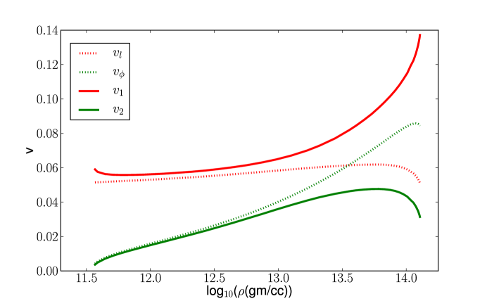
Figure 1: The velocities of the two eigenmodes. The dotted lines are $v_{l}$ and $v_{\phi}$ ignoring mixing.

In terms of the canonically normalized fields the kinetic terms in Fourier space has the form,

$${{\cal{S}}}=\frac{1}{2}\sum_{k}(\tilde{\varphi}(-k)\;\;\hat{{\bf{k}}}.\tilde{\xi}(-k))\left(\begin{array}[]{cc}k_{0}^{2}-v_{\phi}^{2}{\bf{k}}^{2}&g_{\rm mix}k_{0}|{\bf{k}}|\\ g_{\rm mix}k_{0}|{\bf{k}}|&k_{0}^{2}-v_{l}^{2}{\bf{k}}^{2}\end{array}\right)\left(\begin{array}[]{c}\tilde{\varphi}(k)\\ \hat{{\bf{k}}}.\tilde{\xi}(k)\end{array}\right)$$ (68)

The velocities of the two eigenmodes can be obtained by diagonalizing the matrix in Eq. 68. The results are shown in Fig. 1 where the solid curves incorporate mixing effects due to a finite $g_{\rm mix}$ given by Eq. 67 and the dotted curves show the uncoupled case with $g_{\rm mix}=0$.

In contrast, the speed of the transverse lattice modes are unaffected by mixing and is given by

$$v_{t}=\sqrt{\frac{{\mu}}{\rho}}=\sqrt{\frac{{\mu}}{(n_{p}+n_{b})m_{n}}}\,.$$ (69)

Here, only entrainment effects play a role in the propagation of transverse lattice phonons, as was previously pointed out in Ref. [9].

5.2 Crystalline superfluids or LOFF-like phases

Other systems of phenomenological interest where this low energy theory applies are the LOFF phases [5, 6]. Here, attractive interactions between two species of fermions leads to pairing at the Fermi surface but with a pair condensate $\langle\psi_{1}\psi_{2}\rangle$ which is spatially inhomogeneous in the ground state. A mismatch in the Fermi-momenta of the two interacting species in the absence of pairing, disfavors the formation of zero-momentum Cooper pairs and instead pairs with finite total momentum are favored. These pairs condense to form a ground state that breaks translation symmetry and can be written as a sum over plane-waves,

$$\langle\psi_{1}(x)\psi_{2}(x)\rangle\sim\Delta({\bf r})=\Delta\sum_{\{{\bf q}^{a}\}}e^{2i{\bf q}^{a}\cdot{\bf r}}\;,$$ (70)

where $\Delta$ is the gap parameter. The magnitude of the momentum $|{\bf{q}}^{a}|\simeq\delta k_{F}$ where $\delta k_{F}$ is the splitting between the Fermi momenta of the interacting species. The magnitudes of the momenta and their spatial orientation is determined by minimizing the total free energy and this set of momenta specifies a crystalline ground state. The LOFF phases can in principle be realized in cold atomic Fermi gases where a splitting between Fermi levels can be achieved through a population imbalance [28] and in dense quark matter where a Fermi level splitting arises naturally [29, 30].

In dense quark matter, pairing between different flavors of quarks can play a role in determining the ground state structure. The relatively large strange quark mass, and charge neutrality induce a splitting between the Fermi energies of up, down and strange quarks. The expected splitting between the Fermi energies is $\delta\mu\simeq m_{s}^{2}/(8\mu_{q})$ where $m_{s}$ is the strange quark mass and $\mu_{q}$ is the quark chemical potential. At moderate densities, such as those realized in the neutron star core where $\mu_{q}\simeq 400$ MeV, this splitting between Fermi energies can favor LOFF phases in quark matter with spatially varying di-quark condensates with a crystalline structure when $\delta\mu\sim\Delta_{0}/\sqrt{2}$ [31, 32, 33], where $\Delta_{0}$ is the gap in the absence of Fermi surface splitting. As this ground state breaks the same symmetries as those discussed in Section 2, these phases are amenable to the same low energy energy effective theory formulation.

Several aspects of the low energy theory of crystalline phases in quark matter have already been described in Ref. [34]. In Ref. [16], the coefficients of the “lattice only” ($\phi=0$ in Eq. 1) effective theory were computed microscopically in a Ginzburg-Landau expansion [33]. This work was primarily focussed on the shear modes and showed that both the kinetic coefficient, $\rho$, and the elastic constants ${\mu}$ etc., were of the order $\mu_{q}^{2}\Delta^{2}$ where $\Delta$ is the pairing gap parameter. The mixing between the longitudinal lattice phonon mode and the superfluid mode was mentioned but the relevant mixing coefficient was not calculated. Using the same techniques, we have estimated the mixing coefficient and we find that in the regime where LOFF-like phases are favored

$$g^{\rm LOFF}_{\rm mix}\sim\frac{\Delta}{\delta\mu}\,.$$ (71)

Similarly, the coefficients for the “superfluid only” ($\xi^{a}=0$) sector can also be computed (some were calculated in [35]). For $\Delta\ll\mu_{q}$ we expect the coefficient $f_{\phi}^{2}\sim\mu_{q}^{2}$, corresponding to the density of states near the Fermi surface for a relativistic system. Our simple estimates here show that strong mixing between the superfluid and the longitudinal mode can be realized, with important implications for hydrodynamic oscillations both in the context of dense quark matter and trapped imbalanced Fermi gases, where LOFF phases may also be potentially realized. Definitive results require a rigorous derivation of the low-energy constants and such a calculation is being pursued and will be reported elsewhere.

6 Conclusions

We have studied a low energy effective theory describing phases of matter that simultaneously break translational symmetry and a number conservation symmetry. $U(1)$ phase invariance and general coordinate invariance restrict the combinations of terms that can appear in the effective lagrangian. We have shown that the lowest order lagrangian (featuring equal number of derivatives and Goldstone fields) is determined by the derivatives of the thermodynamic pressure with respect to the external fields such as the chemical potential. While this was known in the case of one superfluid system [14, 15], here we have provided a different proof for superfluids and we have generalized it to the mixed system. The two main results of this paper, Eqs. 49 and 57, provide a useful framework for computing the low energy dynamics.

Our thermodynamic matching relates the LECs to thermodynamic derivatives of the free energy with respect to external fields (chemical potential, vector potential, background metric). We have also pointed out the relation between LECs and correlators of the $U(1)$ current and the stress tensor at small momenta. Both approaches might be pursued in future non-perturbative calculations using many-body techniques such as Skyrme Hatree-Fock and Quantum Monte Carlo.

As a concrete example of phenomenological interest, we have considered matter in the inner crust of a neutron star, updating a previous estimate of the parameter characterizing the kinetic mixing of superfluid and lattice phonons. We also discussed briefly how this formulation would apply to the crystalline superfluids or LOFF-like phases and highlighted the role of mixing between the modes in these systems.

Finally, we note that the formalism that we have set up here can be applied to study the low-energy dynamics of other physical systems with several spontaneously broken symmetries, such as a system composed of two superfluid species.

Acknowledgements We thank Tanmoy Bhattacharya, Nicolas Chamel, Michael Forbes, Michael Graesser, Emil Mottola, Chris Pethick, and Dam Son for useful discussions at various stages of this work. We thank Krishna Rajagopal and Massimo Mannarelli for comments and suggestions on the manuscript. This work was supported by grants from the department of energy DE-AC52-06NA25396 (LANL), and the DOE topical collaboration to study of Neutrinos and nucleosynthesis in hot and dense matter.

Appendix A $\Omega[{\bar{A}}^{n},{\bar{A}}^{p},{\bar{g}}]$ and energy density of deformed states

In this appendix we show that the energy density $\Omega[{\bar{A}}^{n},{\bar{A}}^{p},{\bar{g}}]=-W[{\bar{A}}^{n},{\bar{A}}^{p},{\bar{g}}]/(VT)$ calculated using the path integral (Eqs. 29 and 40) admits a simple physical interpretation. It is the expectation value per unit volume ${\cal E}[\zeta_{g}]=\langle\Omega_{g}|\hat{H}_{{\bar{A}}^{n},{\bar{A}}^{g},{\bar{g}}=\eta}|\Omega_{g}\rangle/V$ of the flat-space Hamiltonian in the state $|\Omega_{g}\rangle$ that minimizes ${\cal E}[\zeta_{g}]$ subject to the constraint $\langle\Omega_{g}|\xi^{a}(x)|\Omega_{g}\rangle=\zeta_{g}^{a}(x)$, with $\zeta_{g}^{a}(x)$ satisfying ${\bar{g}}_{ab}=\eta_{ab}-2s_{ab}(\zeta)$ (see Eq. 51). In other words $\Omega[{\bar{A}}^{n},{\bar{A}}^{p},{\bar{g}}]$ is the energy density in the lowest energy state subject to the “deformation condition” $\langle\Omega_{g}|\xi^{a}(x)|\Omega_{g}\rangle=\zeta_{g}^{a}(x)$. It is precisely in this sense one should think of the metric ${\bar{g}}_{ab}$ as determining the shape of the system. To avoid notational clutter, we will focus here on the case of a pure solid system and neglect the dependence on the external fields ${\bar{A}}^{n}$ and ${\bar{A}}^{p}$. The derivation involves several steps, which we summarize below.

• First, let us evaluate the partition function in the presence of a space-time independent background metric $\bar{g}_{\mu\nu}$ of form Eq. 53 by the saddle point method. The classical solution that minimizes the Euclidean action and is well behaved at $|x|\rightarrow\infty$ is given by $\xi^{a}=0$. So we have:

  $$Z[{\bar{g}}]=e^{iW[{\bar{g}}]} = {\rm Exp}\left\{iVT\,{\cal L}_{0}\Big{(}H^{ab}(g={\bar{g}},\xi=0)\Big{)}\right\}$$ (72)

• Since we are working with a diffeomorphism invariant theory, we can obtain the same result for the free energy in a different coordinate system. Let us use this freedom to switch from coordinates $(x^{a},{\bar{g}}_{ab})$ to the “flat” coordinates $(\tilde{x}^{a},\eta_{ab})$. The appropriate variable transformation can be found by noting that $H^{ab}$ is a scalar density. This results in $x^{a}(\tilde{x})=\tilde{x}^{a}-\xi^{a}_{g}(\tilde{x})$, with the field $\xi_{g}$ determined by the condition $H^{ab}(g={\bar{g}},\xi=0)=H^{ab}(g=\eta,\xi=\xi_{g})$, which explicitly reads

  $${\bar{g}}^{ab}=\eta^{ab}-\Big{(}\frac{\partial\xi_{g}^{b}}{\partial{\tilde{x}_{a}}}+\frac{\partial\xi_{g}^{a}}{\partial\tilde{x}_{b}}-\eta^{ij}\frac{\partial\xi^{a}_{g}}{\partial\tilde{x}_{i}}\,\frac{\partial\xi^{b}_{g}}{\partial\tilde{x}_{j}}\,\Big{)}~{}.$$ (73)

  Eq. 73 defines $\xi_{g}^{a}$ up to rigid rotations and translations. For constant ${\bar{g}}_{ab}$ the solution has the form $\xi_{g}^{a}(\tilde{x})=K^{a}_{b}\tilde{x}^{b}+c^{a}$ where the elements of $K^{a}_{b}$ and $c^{a}$ are constant . Equivalently the inverse change of variables reads $\tilde{x}^{a}(x)=x^{a}+\zeta^{a}_{g}(x)$, with $\zeta^{a}_{g}(x)=\xi^{a}_{g}(\tilde{x})+O(\xi_{g}^{2})$, and one has ${\bar{g}}_{ab}=\eta_{ab}-2s_{ab}(\zeta)$, with the strain $s_{ab}(\zeta)$ given in Eq. 51.
  In summary, as a consequence of general coordinate invariance one has:

  $$Z[{\bar{g}}]=e^{iW[{\bar{g}}]} = {\rm Exp}\left\{iVT\,{\cal L}_{0}\Big{(}H^{ab}(g=\eta,\xi=\zeta_{g})\Big{)}\right\}~{},$$ (74)

  with a time-independent field configuration $\zeta_{g}(\vec{x})$ determined by Eqs. 51 or alternatively 73.

• Next we note that the exponent on the RHS of Eq. 74 is the flat-space action evaluated at the field $\xi=\zeta_{g}$. Moreover, to leading order in the loop expansion (and low-energy expansion) the action coincides with the quantum effective action $\Gamma[\zeta_{g}]={\cal S}_{\rm eff}[\zeta_{g}]$. But the quantum effective action $\Gamma[\zeta_{g}]$ admits an energy interpretation [36, 37, 38]: for time-independent field configurations $\zeta_{g}(\vec{x})$, one has that $\Gamma[\zeta_{g}]/T=-\,\langle\Omega_{g}|\hat{H}_{{\bar{A}}^{n},{\bar{A}}^{g},{\bar{g}}=\eta}|\Omega_{g}\rangle$ where $|\Omega_{g}\rangle$ is the state that minimizes the expectation value of the Hamiltonian under the constraint $\langle\Omega_{g}|\hat{\xi}^{a}(x)|\Omega_{g}\rangle=\zeta_{g}^{a}(\vec{x})$ . In equations, the above chain of reasoning reads

  $$W[{\bar{g}}] \equiv -VT\,\Omega[{\bar{g}}]$$ (75)

  $$W[{\bar{g}}] = {\cal S}_{\rm eff}[\zeta_{g}]=\Gamma[\zeta_{g}]=-T\,\langle\Omega_{g}|\hat{H}_{{\bar{A}}^{n},{\bar{A}}^{g},{\bar{g}}=\eta}|\Omega_{g}\rangle$$ (76)

  $$\equiv -VT\,{\cal E}[\zeta_{g}]~{},$$ (77)

  thus proving that $\Omega[{\bar{g}}]={\cal E}[\zeta_{g}]$, with $\zeta_{g}$ related to ${\bar{g}}_{ab}$ by $\bar{g}_{ab}=\eta_{ab}-2s_{ab}(\zeta_{g})$.

References

• [1] M. Baldo, U. Lombardo, E. E. Saperstein, and S. V. Tolokonnikov. The role of superfluidity in the structure of the neutron star inner crust. Nuclear Physics A, 750:409–424, April 2005.
• [2] B. Carter, N. Chamel, and P. Haensel. Entrainment coefficient and effective mass for conduction neutrons in neutron star crust: simple microscopic models. Nuclear Physics A, 748(3-4):675 – 697, 2005.
• [3] B. Carter, N. Chamel, and P. Haensel. Entrainment Coefficient and Effective Mass for Conduction Neutrons in Neutron Star Crust:. Macroscopic Treatment. International Journal of Modern Physics D, 15:777–803, 2006.
• [4] A. F. Andreev and I. M. Lifshitz. Quantum theory of crystal defects. Soviet Physics-JETP., 29:1107, 1969.
• [5] P. Fulde and R. A. Ferrell. Superconductivity in a strong spin-exchange field. Phys. Rev., 135(3A):A550–A563, 1964.
• [6] A. I. Larkin and Yu. N. Ovchinnikov. Inhomogeneous state of superconductors. Soviet Physics-JETP., 20:762–769, 1965.
• [7] E. Kim and M. H. W. Chan. Probable observation of a supersolid helium phase. Nature, 427:225–227, 2004.
• [8] D. T. Son. Effective lagrangian and topological interactions in supersolids. Phys. Rev. Lett., 94(17):175301, 2005.
• [9] C. J. Pethick, N. Chamel, and S. Reddy. Superfluid Dynamics in Neutron Star Crusts. Progress of Theoretical Physics Supplement, 186:9–16, 2010.
• [10] D. N. Aguilera, V. Cirigliano, J. A. Pons, S. Reddy, and R. Sharma. Superfluid heat conduction and the cooling of magnetized neutron stars. Phys. Rev. Lett., 102(9):091101, 2009.
• [11] T. E. Strohmayer and A. L. Watts. The 2004 Hyperflare from SGR 1806-20: Further Evidence for Global Torsional Vibrations. Astrophys. J., 653:593–601, 2006.
• [12] Alexandros Gezerlis and J. Carlson. Strongly paired fermions: Cold atoms and neutron matter. Phys. Rev. C, 77(3):032801, 2008.
• [13] Roberto Anglani, Massimo Mannarelli, and Marco Ruggieri. Collective modes in the color flavor locked phase. hep-ph/1101.4277, 2011.
• [14] D. T. Son. Low-energy quantum effective action for relativistic superfluids. hep-ph/0204199, 2002.
• [15] D. T. Son and M. Wingate. General coordinate invariance and conformal invariance in nonrelativistic physics: Unitary Fermi gas. Annals of Physics, 321(1):197 – 224, 2006. January Special Issue.
• [16] Massimo Mannarelli, Krishna Rajagopal, and Rishi Sharma. Rigidity of crystalline color superconducting quark matter. Phys. Rev. D, 76(7):074026, 2007.
• [17] H. Leutwyler. Nonrelativistic effective Lagrangians. Phys. Rev., D49:3033–3043, 1994.
• [18] S. Weinberg. Phenomenological lagrangians. Physica A: Statistical and Theoretical Physics, 96(1-2):327 – 340, 1979.
• [19] M. Greiter, F. Wilczek, and E. Witten. Hydrodynamic Relations in Superconductivity. Modern Physics Letters B, 3:903–918, 1989.
• [20] Massimo Mannarelli and Cristina Manuel. Bulk viscosities of a cold relativistic superfluid: color- flavor locked quark matter. Phys. Rev., D81:043002, 2010.
• [21] H. Leutwyler. Phonons as Goldstone bosons. Helv. Phys. Acta, 70:275–286, 1997.
• [22] L. D. Landau and E. M. Lifshitz. Theory of Elasticity. Course of theoretical physics by L. D. Landau and E. M. Lifshitz, Vol. 6. Butterworth-Heinemann, 3 edition, 1986.
• [23] D. C. Wallace. Thermoelasticity of stressed materials and comparison of various elastic constants. Phys. Rev., 162(3):776–789, 1967.
• [24] J. R. Ray. Effective elastic constants of solids under stress: Theory and calculations for helium from 11.0 to 23.6 GPa. Phys. Rev. B, 40(1):423–430, 1989.
• [25] N. Chamel. Band structure effects for dripped neutrons in neutron star crust. Nuclear Physics A, 747:109–128, January 2005.
• [26] W. G. Newton, J. R. Stone, and A. Mezzacappa. From microscales to macroscales in 3D: selfconsistent equation of state for supernova and neutron star models. Journal of Physics Conference Series, 46:408–412, 2006.
• [27] N. Chamel. Effective mass of free neutrons in neutron star crust. Nuclear Physics A, 773:263–278, 2006.
• [28] R. Combescot. Introduction to FFLO phases and collective mode in the BEC-BCS crossover. ArXiv Condensed Matter e-prints, February 2007.
• [29] Roberto Casalbuoni and Giuseppe Nardulli. Inhomogeneous superconductivity in condensed matter and QCD. Rev. Mod. Phys., 76(1):263–320, 2004.
• [30] Mark G. Alford, Andreas Schmitt, Krishna Rajagopal, and Thomas Schäfer. Color superconductivity in dense quark matter. Rev. Mod. Phys., 80(4):1455–1515, 2008.
• [31] Mark G. Alford, Jeffrey A. Bowers, and Krishna Rajagopal. Crystalline color superconductivity. Phys. Rev., D63:074016, 2001.
• [32] Jeffrey A. Bowers and Krishna Rajagopal. The crystallography of color superconductivity. Phys. Rev., D66:065002, 2002.
• [33] Krishna Rajagopal and Rishi Sharma. Crystallography of three-flavor quark matter. Phys. Rev. D, 74(9):094019, 2006.
• [34] R. Casalbuoni, Raoul Gatto, M. Mannarelli, and G. Nardulli. Effective field theory for the crystalline colour superconductive phase of QCD. Phys. Lett., B511:218–228, 2001.
• [35] R. Gatto and M. Ruggieri. On the ground state of gapless two flavor color superconductors. Phys. Rev., D75:114004, 2007.
• [36] K. Symanzik. Renormalizable models with simple symmetry breaking. 1. Symmetry breaking by a source term. Commun. Math. Phys., 16:48–80, 1970.
• [37] S. R. Coleman. Secret Symmetry: An Introduction to Spontaneous Symmetry Breakdown and Gauge Fields. Subnucl. Ser., 11:139, 1975.
• [38] S. Weinberg. The quantum theory of fields. Vol. 2: Modern applications. Univ. Pr., Cambridge, UK, 1996.