Energy Efficiency and Goodput Analysis in Two-Way Wireless Relay Networks

Abstract

In this paper, we study two-way relay networks (TWRNs) in which two source nodes exchange their information via a relay node indirectly in Rayleigh fading channels. Both Amplify-and-Forward (AF) and Decode-and-Forward (DF) techniques have been analyzed in the TWRN employing a Markov chain model through which the network operation is described and investigated in depth. Automatic Repeat-reQuest (ARQ) retransmission has been applied to guarantee the successful packet delivery. The bit energy consumption and goodput expressions have been derived as functions of transmission rate in a given AF or DF TWRN. Numerical results are used to identify the optimal transmission rates where the bit energy consumption is minimized or the goodput is maximized. The network performances are compared in terms of energy and transmission efficiency in AF and DF modes.

I Introduction

Recently, there has been much interest on two-way relay networks (TWRNs) in which two source nodes $T_{1}$ and $T_{2}$ without a direct link communicate with each other via a relay node. The architecture of TWRNs makes it possible to better exploit the channel multiplexing of uplink and downlink wireless medium [1]. The source nodes initially send their data to the relay node. The received data is combined employing a certain method according to the Amplify-and-Forward (AF) or the Decode-and-Forward (DF) mode and gets broadcasted from the relay back to both source nodes. With the application of network coding and channel estimation techniques [2], $T_{1}$ and $T_{2}$ can perform self-interference cancelation and remove their own transmitted codewords from the received signal. Four time slots needed in a traditional one-way transmission for the forward and backward channels to accomplish one-round information exchange between $T_{1}$ and $T_{2}$ via the relay node can be reduced to two in TWRNs by comparison.

In a realistic multi-user wireless network, e.g. IS-856 system [3] which has more relaxed delay requirements, the transmission power is fixed while the rate can be adapted according to the channel conditions. Moreover, Automatic Repeat reQuest (ARQ) techniques have been applied to improve the transmission reliability above the physical layer [4]. Prior works [5], [6] also show there is a compromise between transmission rate $R$ and ARQ such that the network average successful throughput, i.e., the goodput, can be maximized at an optimal rate $R^{*}$. In addition to the goodput analysis, we in this paper are interested in energy-efficient operation. In such cases, the energy consumption due to retransmission should also be taken into account to evaluate the energy efficiency with respect to $R$. Hence, we investigate the joint optimization of $R$ (at the physical layer) and the number of ARQ retransmissions (at the data-link layer) by adopting a cross-layer framework in TWRNs.

The remainder of this paper is organized as follows. Section II introduces the TWRN model, channel assumptions as well as its general working mechanism. In Sections III and IV, we investigate the Markov chain model under both AF and DF modes to derive the analytical expressions for the bit energy consumption and goodput. In Section V, the numerical results are shown to compare the system performance in AF and DF modes. Section VI provides the conclusion.

II System Formulation and Channel Assumptions

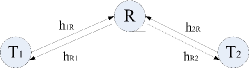
Figure 1: Two-Way Relay Network

In Figure 1, we depict a 3-node TWRN where source nodes $T_{1}$ and $T_{2}$ can only exchange information via the relay node. Codewords $x_{1}$ and $x_{2}$ from $T_{1}$ and $T_{2}$, respectively, have equal length and unit energy. All nodes are working in half-duplex mode and the channels between $T_{1}$ and the relay, and $T_{2}$ and the relay are modeled as complex Gaussian random variables with distributions $h_{1r}\sim{\mathcal{CN}(0,\sigma_{1}^{2})}$ and $h_{2r}\sim{\mathcal{CN}(0,\sigma_{2}^{2})}$. Without loss of generality, we also assume channel reciprocity such that $h_{r1}$ and $h_{r2}$ have identical distributions as $h_{1r}$ and $h_{2r}$, respectively. Odd and even time slots have equal length, which is the time to transmit one codeword, and are dedicated for uplink and downlink data transmissions, respectively. ACK and NACK control packets are assumed to be always successfully received and the trivial processing time is ignored. Additive Gaussian noise at the receiver terminals is modeled as $n\sim{\mathcal{CN}(0,\sigma_{n}^{2})}$.

There are two more key assumptions: 1) channel codes support communication at the instantaneous channel capacity levels, and outages, which occur if transmission rate exceeds the instantaneous channel capacity, lead to packet errors and are perfectly detected at the receivers; 2) depending on whether packets are successfully received or not, ACK or NACK control frames are sent and received with no errors. Based on above network formulations, we can further discuss the TWRN working procedure according to the current network states under AF and DF relay schemes, and find out the inherent impact of the transmission rate $R$ on network performances.

III Amplify-and-Forward TWRN

III-A Network Model

The TWRN in AF mode can be visualized as two bi-directional cascade channels where in the odd time slots, $T_{1}$ and $T_{2}$ send individual codewords simultaneously to the relay and the signals are actually superimposed in the wireless medium. The relay will then amplify the received signals proportional to the average received power and broadcast the combined signals back to $T_{1}$ and $T_{2}$ in the even time slots.

According to Fig.1, the received signals at the relay in odd time slots is

$$y_{r}=\sqrt{P_{1}}h_{1r}x_{1}+\sqrt{P_{2}}h_{2r}x_{2}+n,$$ (1)

where $P_{1}$, $P_{2}$ are the transmit power of $T_{1}$ and $T_{2}$ respectively. The relay will forward $y_{r}$ with a scaling factor $\beta$ which is

$$\beta=\frac{\sqrt{P_{r}}}{\sqrt{P_{1}\sigma_{1}^{2}+P_{2}\sigma_{2}^{2}+\sigma_{n}^{2}}}.$$ (2)

where $P_{r}$ is the relay’s transmit power.

Here, we normalize the variance of the channel between $T_{1}$ and $T_{2}$ as $\sigma^{2}=1$ and by using a normalized distance factor [7] $k=\frac{d_{T_{1},Relay}}{d_{T_{1},T_{2}}}\in(0,1)$ while assuming the variances of the other links are proportional to $d^{-\alpha}$ where $\alpha$ is the path loss coefficient, we then have $\sigma_{1}^{2}=k^{-\alpha}\sigma^{2}$ and $\sigma_{2}^{2}=(1-k)^{-\alpha}\sigma^{2}$. At the end of even time slots, the received signals on $T_{1}$ and $T_{2}$ can be written as

$$y_{1} =\sqrt{P_{1}}\beta h_{r1}h_{1r}x_{1}+\sqrt{P_{2}}\beta h_{r1}h_{2r}x_{2}+\beta h_{r1}n+n_{1}$$

$$y_{2} =\sqrt{P_{1}}\beta h_{r2}h_{1r}x_{1}+\sqrt{P_{2}}\beta h_{r2}h_{2r}x_{2}+\beta h_{r2}n+n_{2},$$ (3)

where $n_{1}$, $n_{2}$, and $n$ are i.i.d Gaussian noise components. Assuming the instantaneous channel state information is perfectly known at $T_{1}$ and $T_{2}$, the self-interference part can be removed from $y_{1}$ and $y_{2}$ and the signals for decoding can be represented by

$$\widehat{y}_{1} =\sqrt{P_{2}}\beta h_{r1}h_{2r}x_{2}+\beta h_{r1}n+n_{1}$$

$$\widehat{y}_{2} =\sqrt{P_{1}}\beta h_{r2}h_{1r}x_{1}+\beta h_{r2}n+n_{2}.$$ (4)

The cascade channel instantaneous rate from $T_{1}$ to $T_{2}$ and from $T_{2}$ to $T_{1}$ are hence represented by

$$R_{12} =\log\left(1+\frac{|\beta h_{r2}h_{1r}|^{2}P_{1}}{(1+|\beta h_{r2}|^{2})\sigma_{n}^{2}}\right)$$

$$R_{21} =\log\left(1+\frac{|\beta h_{r1}h_{2r}|^{2}P_{2}}{(1+|\beta h_{r1}|^{2})\sigma_{n}^{2}}\right).$$ (5)

To describe the network mechanism more accurately, we need to formulate the protocol of TWRN in AF mode as follows:

1. Each transmission round contains two consecutive time slots. In the odd slot, source nodes $T_{1}$ and $T_{2}$ both transmit codewords to the relay with transmission rate $R$ bit/sec/Hz, and the relay in the following even slot broadcasts $\beta y_{r}$ back to source nodes.

2. At the end of one transmission round, $T_{1}$ and $T_{2}$ perform self-interference cancelation (SIC) to subtract their own weighted messages, and decode $\widehat{y}_{1}$ and $\widehat{y}_{2}$, respectively. If the decoding fails, an outage event will be declared on that cascade link.

3. The outage event on the cascade link $T_{1}-T_{2}$ (or $T_{2}-T_{1}$) is defined as the probability of the event $R_{12}<R$ (or $R_{21}<R$). ACK or NACK packets would be sent back to the relay based on successful transmission or outage. The relay will also notify $T_{1}$ and $T_{2}$ whether a new codeword or an old codeword should be (re)transmitted in the next odd time slot with the control packet information.

The network state transition diagram of the AF TWRN can be modeled as a Markov chain as shown in Fig. 2, where the probability on each path denotes the probability of the transition between two states. $p_{12}$ and $p_{21}$ are defined as the outage probabilities on the cascade $T_{1}-T_{2}$ and $T_{2}-T_{1}$ links and are given by

$$p_{12} =p(R_{12}<R)=p\left(\frac{|h_{r2}h_{1r}|^{2}}{\frac{1}{\beta^{2}}+|h_{r2}^{2}|}<\frac{(2^{R}-1)\sigma_{n}^{2}}{P_{1}}\right)$$ (6)

$$p_{21} =p(R_{21}<R)=p\left(\frac{|h_{r1}h_{2r}|^{2}}{\frac{1}{\beta^{2}}+|h_{r1}^{2}|}<\frac{(2^{R}-1)\sigma_{n}^{2}}{P_{2}}\right).$$ (7)

(6) and (7) can be determined using the cumulative distribution function of the random variable $X$ [8]

$$F_{X}(x) =1-\frac{1}{\mu_{2}}\int_{0}^{\infty}e^{-\frac{x(a+z)}{\mu_{1}z}-\frac{z}{\mu_{2}}}dz$$ (8)

where

$$X =\frac{Y_{1}Y_{2}}{a+Y_{2}},$$ (9)

and $Y_{1}$ and $Y_{2}$ are independent exponential distributed with mean $\mu_{1}$ and $\mu_{2}$, and $a$ is a constant. In this context, we know

$$\left\{\begin{array}[]{l}\mu_{1}=E[|h_{1r}|^{2}],\,\hskip 8.5359pt\mu_{2}=E[|h_{r2}|^{2}],\hskip 8.5359ptfor\hskip 8.5359ptp_{12}\\ \mu_{1}=E[|h_{2r}|^{2}],\,\hskip 8.5359pt\mu_{1}=E[|h_{r1}|^{2}],\hskip 8.5359ptfor\hskip 8.5359ptp_{21}\\ \alpha=\frac{1}{\beta^{2}}\end{array}\right.$$ (13)

With the given network parameters, $p_{12}$ and $p_{21}$ can be derived accordingly.

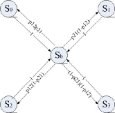
Figure 2: Markov Chain of TWRN in AF

III-B Goodput Analysis

In Fig. 3, it is explicitly seen at the beginning of each odd time slot that both $T_{1}$ and $T_{2}$ transmit to the relay such that at the beginning of each even time slot, the relay is always in the ready-for-broadcasting state $S_{b}$ and will consequently transition to $S_{0}$, $S_{1}$, $S_{2}$, or $S_{3}$ with certain probabilities.

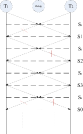
Figure 3: State Transition of TWRN in AF

We first determine the following four equations according to the state transitions in the Markov chain to derive the probability of each state:

$$\begin{cases}p(S_{0})=p(S_{b})p_{12}p_{21}\\ p(S_{1})=p(S_{b})p_{21}(1-p_{12})\\ p(S_{2})=p(S_{b})p_{12}(1-p_{21})\\ p(S_{3})=p(S_{b})(1-p_{21})(1-p_{12})\\ p(S_{0})+p(S_{1})+p(S_{2})+p(S_{3})+p(S_{b})=1.\end{cases}$$ (14)

After solving the set of equations in (14), we obtain $p(S_{b})=\frac{1}{2}$. We know from the inherent characteristics of the AF TWRN that the data exchange only happens in the broadcasting phases with successful packet delivery. Therefore, the system goodput is defined similarly as in [1] by

$$\eta_{AF}$$

$$=p(S_{b})R(2(1-p_{12})(1-p_{21})+p_{12}(1-p_{21})+p_{21}(1-p_{12}))$$

$$=\frac{R(2-p_{12}-p_{21})}{2}.$$ (15)

(III-B) indicates through the terms $p_{12}$ and $p_{21}$ that a higher transmission rate $R$ will result in higher packet error rates (outage), leading to more ARQ retransmissions which equivalently reduce the data rate. Intuitively, a balance between transmission rate and the number of ARQ retransmissions needs to be found such that the goodput is maximized.

III-C Average Bit Energy Consumption

Energy efficiency has always been a major concern in wireless networks. Recently, power or energy efficiency in wireless one-way relay networks have been extensively studied. In [9], the average bit energy consumption $E_{b}$ is minimized by determining the optimal number of bits per symbol, i.e., the constellation size, in a specific modulation format. Similarly as in one-way relay channels, the outage probabilities in TWRNs are functions of the transmission rate $R$. For instance, there could be an increased number of outage events on the cascade channels when codewords are transmitted at a high rate. In such a case, more retransmissions and higher energy expenditure are needed to accomplish the reliable packet delivery. Therefore, we are interested in a possible realization of TWRN operation, which can provide a well-balanced performance on both the goodput $\eta$ and the required energy. We evaluate this by formulating the average bit energy consumption $E_{b}$ required for successfully exchanging one information bit between $T_{1}$ and $T_{2}$.

We then evaluate $E_{b}$ by considering long-term transmissions on TWRN. Regardless of the previous state, whenever the relay is in state $S_{b}$ and is broadcasting, the resulting state would be any of the other four states previously described. Assuming there are $K$ rounds of two-way transmission, each of which consists of a pair of consecutive time slots and each codeword has $L$ bits. Therefore, with $\sum_{i=0}^{3}K_{i}=K$, where $K_{i}$ is the number of transmission round corresponding to state $S_{i}$, the average bit energy consumption could be derived as the ratio of total bits successfully exchanged over total energy consumption:

$$E_{b} =\lim_{K\rightarrow\infty}\frac{K(P_{1}+P_{2}+P_{r})\frac{L}{R}}{K_{3}2L+K_{1}L+K_{2}L}$$

$$=\lim_{K\rightarrow\infty}\frac{(P_{1}+P_{2}+P_{r})\frac{L}{R}}{\frac{K_{3}}{K}2L+\frac{K_{1}}{K}L+\frac{K_{2}}{K}L}$$

$$=\frac{P_{1}+P_{2}+P_{r}}{(2-p_{12}-p_{21})R}.$$ (16)

IV Decode-and-Forward TWRN

IV-A Network Model

The DF TWRN differs from the AF TWRN in that there is a crucial intermediate decoding procedure at the the relay when it has received the codeword from the uplink transmission. If both source nodes are allowed to send codewords to the relay simultaneously in the uplink transmission, the decoding at the relay has to deal with the multiple access problem in a realistic application, with successive interference cancelation techniques. To reduce the hardware complexity and increase the feasibility of implementation, we hereby adopt the DF TWRN mode from [1] where the relay performs sequential Decode-and-Forward. The outage probabilities on $T_{1}-Relay$, $T_{2}-Relay$, $Relay-T_{1}$, $Relay-T_{2}$ links are denoted as $p_{1r}$, $p_{2r}$, $p_{r1}$ and $p_{r2}$. The protocol for sequential DF TWRN is described as follows:

1. In the initial state $S_{0}$, the relay’s buffer is empty and the relay first polls on $T_{1}$ until it receives codeword $x1$ successfully with probability $1-p_{1r}$. Then, the state moves to $S_{1}$ which means the relay holds $x_{1}$ in the buffer. Otherwise, the state remains as $S_{0}$ with probability $p_{1r}$.

2. If the relay already has $x_{1}$, it starts polling $T_{2}$. The state $S_{1}$ either changes to $S_{3}$ with probability $1-p_{2r}$ upon successfully receiving $x_{2}$, or stays in $S_{1}$ with $p_{2r}$.

3. When the relay has both $x_{1}$ and $x_{2}$, it generates a new codeword $y_{n}=\sqrt{\frac{P_{r}}{2}}x_{1}+\sqrt{\frac{P_{r}}{2}}x_{2}$ according to a Gaussian codebook of $2^{2LR}$ with equal power allocation. Then at rate $R$, it broadcasts to $T_{1}$ and $T_{2}$, which will perform SIC to decode $x_{2}$ and $x_{1}$, respectively. Accordingly, the state will transit to $S_{0}$, $S_{1}$, $S_{2}$ or $S_{3}$ with corresponding probabilities $(1-p_{r1})(1-p_{r2})$, $(1-p_{r2})p_{r1}$, $(1-p_{r1})p_{r2}$ or $p_{r1}p_{r2}$ respectively.

4. At the beginning of next transmission round, the relay will decide to poll a new codeword from $T_{1}$ (or $T_{2}$) based on the previous state being $S_{0}$,$S_{2}$ (or $S_{1}$) or just retransmits the old $y_{n}$ if the previous state was $S_{3}$.

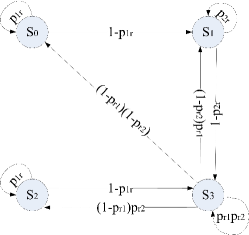
Figure 4: Markov Chain of TWRN in DF

The network state transition diagram of the DF TWRN can be modeled as in Fig. 4 with detailed probabilities on each path. Since the relay receives and decodes $x_{1}$ and $x_{2}$ at different time slots, the received signals at the relay from uplink transmissions can be represented as

$$y_{1r} =\sqrt{P_{1}}h_{1r}x_{1}+n_{1}$$

$$y_{2r} =\sqrt{P_{2}}h_{2r}x_{2}+n_{2}.$$ (17)

Similar to (III-A), the signals for decoding at $T_{1}$ and $T_{2}$ after SIC has been performed can be written as

$$x_{r1} =\sqrt{\frac{P_{r}}{2}}h_{r1}x_{2}+n_{1}$$

$$x_{r2} =\sqrt{\frac{P_{r}}{2}}h_{r2}x_{1}+n_{2}.$$ (18)

IV-B Goodput Analysis

Similarly as in the discussion of the goodput of AF TWRN in Section III, the data exchange only occurs upon the successful signal receptions at $T_{1}$ and $T_{2}$ at the end of the broadcasting time slot. Hence, initially, it is necessary to calculate the probability of being in state stays 3, i.e., $p(S_{3})$.

We start from calculating the outage probabilities on the forward and backward channels as

$$p_{1r} =1-e^{\frac{-(2^{R}-1)\sigma_{n}^{2}}{\mu_{1}P_{1}}}$$

$$p_{2r} =1-e^{\frac{-(2^{R}-1)\sigma_{n}^{2}}{\mu_{2}P_{2}}}$$

$$p_{r1} =1-e^{\frac{-(2^{R}-1)2\sigma_{n}^{2}}{\mu_{1}P_{r}}}$$

$$p_{r2} =1-e^{\frac{-(2^{R}-1)2\sigma_{n}^{2}}{\mu_{2}P_{r}}}.$$ (19)

The probabilities of buffer states can be solved by noting the following relations from Fig. 4:

$$\begin{cases}p(S_{0})=p(S_{0})p_{1r}+p(S_{3})(1-p_{r1})(1-p_{r2})\\ p(S_{1})=p(S_{1})p_{r2}+p(S_{3})(1-p_{r2})p_{r1}\\ p(S_{2})=p(S_{2})p_{1r}+p(S_{3})(1-p_{r1})p_{r2}\\ p(S_{3})=p(S_{3})p_{r1}p_{r2}+p(S_{1})(1-p_{2r})+p(S_{2})(1-p_{1r}).\end{cases}$$ (20)

Solving the equations in (20) with given outage probabilities, we can obtain the following results for the buffer states:

$$\begin{cases}p(S_{0})&=\frac{(1-p_{2r})(1-p_{r1})(1-p_{r2})}{D}\\ p(S_{1})&=\frac{(1-p_{1r})(1-p_{r2})}{D}\\ p(S_{2})&=\frac{(1-p_{2r})(1-p_{r1})p_{r2}}{D}\\ p(S_{3})&=\frac{(1-p_{1r})(1-p_{2r})}{D},\end{cases}$$ (21)

where the polynomial in the denominators is denoted by

$$D =3-2p_{1r}-2p_{2r}-p_{r1}-p_{r2}+p_{r1}p_{2r}+p_{1r}p_{r2}+p_{1r}p_{2r}.$$ (22)

Therefore, the system goodput in the DF mode can be derived as

$$\eta_{DF}$$

$$=p(S_{3})R\left(2(1-p_{r1})(1-p_{r2})+p_{r1}(1-p_{r2})+p_{r2}(1-p_{r1})\right)$$

$$=\frac{R(2-p_{12}-p_{21})(1-p_{1r})(1-p_{2r})}{p_{2r}p_{1r}+p_{r2}p_{1r}+p_{r1}p_{2r}+3-2p_{1r}-2p_{2r}-p_{r1}-p_{r2}}.$$ (23)

IV-C Average Bit Energy Consumption

$E_{b}$ in the DF TWRN is more complicated to calculate than in the AF TWRN where each transmission round has fixed power as can be seen in (III-C). Hence, in the DF scenario, we have to separate the energy expenditure into two parts, energy consumption in the first stage and energy consumption in the second stage. The first stage denotes the state transition from any of 4 previous states to state $S_{3}$, where the relay holds two codewords $x_{1}$ and $x_{2}$ in its buffer and is ready to broadcast. The second stage is that the relay broadcasts its newly generated codeword and the state transits back to any of the four states again.

Considering the relay’s buffer is to be loaded with both codewords $x_{1}$ and $x_{2}$ from any of the previous states on the first stage, the energy consumption conditioned on the previous state $S_{0}$, $S_{1}$, $S_{2}$, or $S_{3}$ on this particular transition will be

$$E_{S_{0}} =\frac{P_{1}L}{(1-p_{1r})R}+\frac{P_{2}L}{(1-p_{2r})R}$$

$$E_{S_{1}} =\frac{P_{2}L}{(1-p_{2r})R}$$

$$E_{S_{2}} =\frac{P_{1}L}{(1-p_{1r})R}$$

$$E_{S_{3}} =0.$$ (24)

On the second stage, the energy consumption for broadcasting is always $\frac{P_{r}L}{R}$, so the average bit energy consumption for one information bit successfully exchanged on the DF TWRN can be computed as

$$E_{b}=\frac{\sum_{i=0}^{3}(E_{S_{i}}+\frac{P_{r}L}{R})p(S_{i})}{(2(1-p_{r1})(1-p_{r2})+(1-p_{r1})p_{r2}+(1-p_{r2})p_{r1})L}$$

$$=\frac{E_{S_{0}}p(S_{0})+E_{S_{1}}p(S_{1})+E_{S_{2}}p(S_{2})+\frac{P_{r}L}{R}}{(2-p_{r1}-p_{r2})L}.$$ (25)

whenever the state probabilities and outage probabilities are known.

V Numerical Results and Comparisons

In this section, we present the numerical results to evaluate the system performance of TWRN in both AF and DF modes. The network configurations are assumed to be as follows: Relay is located in the middle between $T_{1}$ and $T_{2}$ which means $k=0.5$. The power spectrum density of the Gaussian white noise is $\sigma_{n}^{2}=10^{-10}$ and the channel bandwidth is set to $B=10^{6}$ Hz. Path loss coefficient is $\alpha=3.12$ [10]. We also assume the same transmit power for both source nodes and the relay, which is $P_{1}=P_{2}=P_{r}=P$ and define the SNR by $\gamma=\frac{P}{\sigma_{n}^{2}}$.

Firstly, we are particularly interested in how the goodput varies as a function of the transmission rate $R$ at specific SNR values. In Fig. 5, $\eta_{AF}$ and $\eta_{DF}$ are plotted as functions of $R$, with solid and dashed lines corresponding to AF and DF modes, respectively. On each curve with a given specific $\gamma$ value, it’s immediately seen that the goodput first increases within low $R$ range and then begins to drop once the rate is increased beyond the optimal $R^{*}$ which maximizes the goodput $\eta$. Additionally, at low values of the rate $R$, the AF TWRN has higher goodput $\eta_{AF}$, while beyond a certain rate $R$, DF starts to outperform, regardless of the SNR $\gamma$ value.

To better illustrate the goodput performance in AF and DF modes, we look into transmission efficiency by defining a normalized rate $\frac{\eta}{R}$ and plotting it in Fig. 6. The normalized rate is always decreasing when $R$ increases at all SNR’s in both AF and DF. In other words, increasing outage probabilities due to increasing $R$ has eventually resulted in more ARQ retransmissions. Specifically in the high SNR scenario, the normalized rate levels off between 0.6 and 0.7 in AF and 0.9 and 1 in DF, which means the transmission efficiency doesn’t change too much within this rate range. In addition, the AF mode seems to have higher normalized rate in low rate range.

In Fig. 7, we analyze the energy efficiency. We notice that the difference of the average bit energy consumptions between two modes is insignificant up until $R=1$, but DF stills has a better energy efficiency with a lower $E_{b}$ regardless of $\gamma$. However when compared with the corresponding points ($R<1$) in Fig. 6, it is shown that even though DF can achieve a slightly lower $E_{b}$ than AF, it also suffers a lower transmission efficiency in the metric of lower normalized rate. Above $R=1$ in low SNR scenario of $\gamma=0$, AF predominates with both higher normalized rate and lower $E_{b}$ until $R$ approaches about $6$ bits/sec/Hz. Similar results can be observed on the high SNR scenarios also. In Fig. 8, we study the impact of SNR on the normalized rate in both AF and DF. Basically the normalized rate is increasing as SNR increases at all transmission rates. At low SNR e.g. $R=-5\hskip 2.84544ptdB$, DF performs better than AF. As SNR approaches $R=20\hskip 2.84544ptdB$, the normalized rate gets close to 1 (or 0.7) in AF (or DF) mode. Consequently, one way to improve on the transmission efficiency is to increase SNR in the TWRN. Considering overall impacts of rate $R$ and SNR, we can always find an scheme for the TWRN to achieve optimality in respect to the goodput $\eta$, the average bit energy consumption $E_{b}$ or the transmission efficiency.

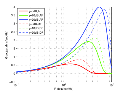
Figure 5: Goodput Vs. Transmission Rate in AF and DF TWRN

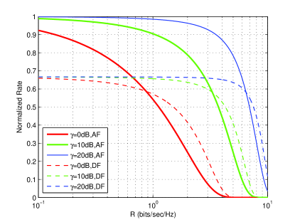
Figure 6: Normalized Transmission Rate Vs. Transmission Rate

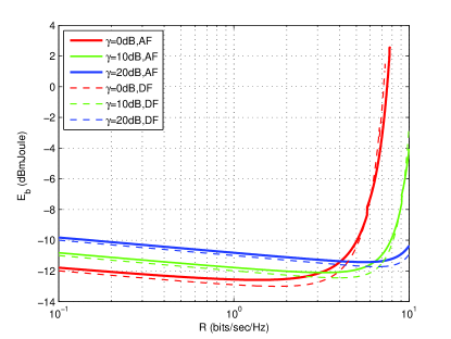
Figure 7: Average Bit Energy Vs. Transmission Rate

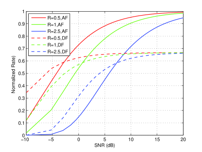
Figure 8: Normalized Transmission Rate Vs. SNR

VI Conclusion

In this paper, we have studied the two-way relay networks working in Amplify-and-Forward and Decode-and-Forward modes. In each mode, we set up a Markov chain model to analyze the state transition in details. ARQ transmission is employed to guarantee the successful packet delivery at the end and mathematical expressions for the goodput and bit energy consumption have been derived. Several interesting results are observed from simulation results: 1) the transmission rate $R$ can be optimized to achieve a maximal goodput in both AF and DF modes; 2) generally the transmission efficiency is higher in AF within a certain $R$ range, while the DF can achieve a slightly higher energy efficiency instead; 3) increasing SNR will always increase the normalized rate regardless of $R$. Hence, it’s possible the network performance be optimized in a balanced manner to maintain a relatively high goodput as well as a low $E_{b}$.

References

- [1] P. Popovski, H. Yomo,“Bi-directional Amplification of Throughput in a Wireless Multi-Hop Network,” IEEE Vehicular Technology Conference 2006, pp. 588 - 593.
- [2] F. Gao, R. Zhang, Y.-C. Liang, “Optimal Channel Estimation and Training Design for Two-Way Relay Networks”, IEEE Trans. Communiction, Vol.57, No. 10, 2009
- [3] D. Tse, P. Viswanath, Fundamentals of Wireless Communication, Cambridge University Press, 2005.
- [4] W. Choi, D. I. Kim, B-H. Kim, “Adaptive multi-node incremental relaying for hybrid-ARQ in AF relay networks”, IEEE Trans. on Wireless Communication, Vol. 9, No. 2, Feb. 2010.
- [5] P. Wu, N. Jindal, “Coding versus ARQ in fading channels: How reliable should the PHY be?”, Globecom 2009.
- [6] R. Aggarwal, P. Schniter, and C. Koksal,“Rate adaptation via linklayer feedback for goodput maximization over a time-varying channel,” IEEE Trans. Wireless Commun., Vol.8, No.8, 2008.
- [7] K. J. Ray Liu, A. K . Sadek, W. Su, A. Kwasinski, Cooperative Communications and Networking, Cambridge University Press, 2009.
- [8] A. Bletsas, Y. Shin and M. Z. Win, “Cooperative Communications with Outage-Optimal Opportunistic Relaying,” IEEE Trans. Wireless Commun., Vol.6, No.9, 2007.
- [9] Q. Chen, M. C. Gursoy, “Energy Efficiency Analysis in Amplify-and-Forward and Decode-and-Forward Cooperative Networks”, IEEE WCNC, Apr. 2010
- [10] V. Erceg, L. J. Greenstein, S. Y. Tjandra, S. R. Parkoff, A. Gupta, B. Kulic, A. A. Julius, and R. Bianchi, “An emperically based path loss model for wireless channels in suburban environments,” IEEE J.Select. Areas Commun, Vol. 17, No. 7, pp.1205-1211, Jul. 1999.