Electron scattering from domain walls in ferromagnetic Luttinger liquids

Abstract

We study the properties of interacting electrons in a one-dimensional conduction band coupled to bulk non-collinear ferromagnetic order. The specific form of non-collinearity we consider is that of an extended domain wall. The presence of ferromagnetic order breaks spin-charge separation and the domain wall introduces a spin-dependent scatterer active over the length of the wall $\lambda$. Both forward and backward scattering off the domain wall can be relevant perturbations of the Luttinger liquid and we discuss the possible low temperature phases. Our main finding is that backward scattering, while determining the ultimate low temperature physics, only becomes important at temperatures $T/J<\exp(-\lambda/\lambda_{+})$ with $J$ being the magnetic exchange and $\lambda_{+}$ the backward scattering length scale. In physical realizations, $\lambda\gg\lambda_{+}$ and the physics will be dominated by forward scattering which can lead to a charge conducting but spin insulating phase. In a perturbative regime at higher temperatures we furthermore calculate the spin and charge densities around the domain wall and quantitatively discuss the interaction induced changes.

I Introduction

In a one-dimensional electron system, particle-like excitations cannot survive in the presence of interactions leading to a breakdown of Fermi liquid theory. Instead, the excitations are of a collective, bosonic nature and can be described by a universal low-energy effective theory, the Luttinger liquid (LL).Tomonaga (1950); Luttinger (1963); Giamarchi (2003) Impurities are expected to play a particularly important role in one dimension, because electrons are not able to circumvent them. Studies have indeed revealed that impurities in many cases are relevant perturbations effectively cutting the chain and therefore impeding transport at low temperatures.Kane and Fisher (1992a); Kane and Fisher (1992b); Eggert and Affleck (1992, 1995); Rommer and Eggert (2000); Sirker et al. (2007, 2008) More surprisingly, however, there are also situations where the low-temperature behavior in the presence of multiple impurities corresponds to “healing”, i.e., to perfect transmission.Eggert and Affleck (1992); Kane and Fisher (1992b)

One of the hallmarks of the Luttinger liquid is spin-charge separation. This means that the normal modes of the Luttinger model have either spin or charge character and are completely decoupled. Spin-charge separation, however, only holds in the case of spin degeneracy. In the presence of a magnetic field—which leads to spin split bands—the normal modes of the Luttinger model acquire a mixed character. This situation was first studied in Refs. Penc and Sólyom, 1993; Frahm and Korepin, 1991 using the Hubbard model in a magnetic field as a starting point. One obvious question to ask is how impurities affect the low temperature properties in such a system. Since spin and charge are no longer decoupled we might expect new low-energy fixed points which are not covered by the standard Kane and Fisher picture.Kane and Fisher (1992b)

Of experimental relevance is, in particular, the case of electrons in a quasi one-dimensional wire coupled to bulk ferromagnetic order. Domain walls in the ferromagnet then act as spatially extended magnetic impurities for the electrons in the wire. Such systems of coupled electronic and magnetic degrees of freedom have received considerable interest,Marrows (2005) spurred, in particular, by possible applications as magnetic domain-wall racetrack memories.Parkin et al. (2008) However, the focus has principally been on how the transport properties of free electrons behave in a ferromagnetic wire with a domain wall, and how these spin polarized currents set the domain wall itself into motion. An interesting question to ask then is whether electron-electron interactions can become important in such cases. Aside from some work on mean-fieldDugaev et al. (2002) and Hartree-FockAraújo et al. (2006, 2007) interactions, there is little consideration in the literature of how the electronic and magnetic behaviour of quasi one-dimensional ferromagnetic systems is modified in a strongly correlated system.

In particular, the case of a ferromagnetic Luttinger liquid with a domain wall present has not yet been fully addressed. In the limit of an infinitely sharp domain wall, Pereira and MirandaPereira and Miranda (2004) have considered an effective low temperature model containing only a spin-flip back scattering term. Based on this model, they have argued that the domain wall scattering in the ultimate low temperature limit is the magnetic analog of the Kane-Fisher problem.Penc and Sólyom (1993); Kane and Fisher (1992b); Eggert and Affleck (1992) In other words at low temperatures either a spin-charge insulator or a Luttinger liquid is found. In addition to the spin-flip back scattering process considered in Ref. [Pereira and Miranda, 2004], however, also a pure potential (spin-independent) back scattering term is allowed by symmetry.Araújo et al. (2006, 2007) By starting from a model for an extended domain wall we will show that such a term is indeed present and can be important for the physics at very low temperatures. Our main focus, however, is what happens in the more physically relevant regime of longer domain walls and higher temperatures. The behaviour of the system in this case remains unknown, and it is that question we wish to address here.

There are three possible temperature regimes in this problem and it is convenient to introduce here some notation for them. At high temperatures we have a “perturbative regime” where the domain wall scattering can be treated as a small perturbation. As we consider lower temperatures the perturbative treatment will break down due to the presence of relevant operators. At first we may still consider the domain wall as an extended region and we refer to this as the “extended regime”. This regime is the focus of our study. At even lower temperatures in the renormalization group flow the domain wall will become effectively delta function like and we can treat the relevant operators as boundary terms. This regime we refer to as the “sharp regime”, and is the regime which has been previously discussed in the literature.Pereira and Miranda (2004); Araújo et al. (2006, 2007) In the sharp regime, the spin-flip and the potential back scattering terms with scattering length $\lambda_{+}$ are the possible relevant perturbations determining the low-temperature physics. We will show, however, that if we start from a system with an extended domain wall with length $\lambda\gg\lambda_{+}$, then temperatures $T/J<\exp(-\lambda/\lambda_{+})$, with $J$ being the magnetic exchange, are required to enter this regime. This regime therefore is only accessible if one already starts with a very sharp domain wall, a situation which can possibly be realized by nanoconstrictions.Bruno (1999)

Experimentally the construction of ferromagnetic chains of single magnetic atoms is already possible.Gambardella et al. (2002) In such systems the ferromagnetic order is observed to extend over small distances separated by regions of non-collinearity.Gambardella et al. (2002); Shen et al. (1997); Elmers et al. (1994); Hauschild et al. (1998); Wiesendanger (2009) It is important to note that these chains are assembled on some substrate and therefore cannot be considered as fully isolated one-dimensional systems. Therefore the Mermin-Wagner theorem,Mermin and Wagner (1966) which forbids long-range ferromagnetic order at finite temperatures in a strictly one-dimensional system with sufficiently short-range interactions, does not apply. Furthermore, the substrate has consequences for the effective spin exchange between the atoms. The spin exchange tensor can quite generally be decomposed into a symmetric and an antisymmetric part. In spin chains which are part of a regular three-dimensional crystal the antisymmetric part is often forbidden by inversion symmetry. For chains of single magnetic atoms on a substrate, on the other hand, both terms are expected to be present so that non-collinear spin order is a generic property of such systems. The presence of the substrate might also disguise the Luttinger liquid properties of the atomic wire and our model system might therefore be too simplistic to directly apply to this situation. Nevertheless, it might serve as a starting point for the investigation of more realistic models.

Other possible candidates our model might apply to include dilute magnetic semiconductors,Jungwirth et al. (2006) and low temperature ferromagnetic metals.Natelson et al. (2000); Granitzer et al. (2007) Systems where the magnetic and electronic degrees of freedom belong to different layers would also be a possible realization. Furthermore, we want to point out that our analysis is also valid for a quantum wire with a non-uniform external magnetic field applied.

Our paper is organized as follows: In Sec. II we introduce the model and derive the low-energy effective theory by linearizing the excitation spectrum followed by bosonization. In Sec. III we consider the first order renormalization group (RG) equations for the various scattering processes and discuss the fixed points of the RG flow in the extended and sharp regimes. In Sec. IV we study an experimentally accessible temperature regime where the relevant scattering terms can be treated perturbatively. We discuss different cases depending on the hierarchy of the different length scales present in the problem and calculate the spin and charge densities around the domain wall. In the final section we present a brief summary of our results and some additional conclusions.

II The Model

We will consider an “s-d” like model in which the bulk magnetization and the conduction electrons are treated separately (though of course still coupled). We assume two timescales in the problem, a fast electronic one and a slow magnetic one. This allows us to answer the question of how the presence of the domain wall affects the Luttinger liquid, forgetting the effect the motion of the domain wall will have on the conduction electrons. For the already mentioned dilute magnetic semiconductors and, in particular, ferromagnetic metals this model with separate electronic and magnetic degrees of freedom, active on different time scales, is a realistic starting point.

The direction of the bulk magnetization of the wire can be described by a unit vector $\vec{n}(z)=\cos[\Theta(z)]\hat{\mathbf{z}}+\sin[\Theta(z)]\hat{\mathbf{y}}$ and we consider, in particular, the case $\cos[\Theta(z)]=-\tanh[z/\lambda]$ describing the spatial profile of a domain wall of length $\lambda$ situated at $z=0$, this is plotted schematically in Fig. 1. The magnetization is coupled to the conduction band electrons with a strength given by the exchange coupling $J$. We consider a screened, and hence short range, interaction $V(z-z^{\prime})$. To simplify the presentation we consider here a spin-independent, $SU(2)$ symmetric interaction. We want to point out, however, that the low-energy theory, Eqs. (3) and (4), obtained after linearizing the excitation spectrum remains valid for a spin-dependent interaction $V_{\sigma\sigma^{\prime}}(z-z^{\prime})$ as long as the interaction is spin conserving.

We start from the following standard “s-d” Hamiltonian,Blundell (2009) $\tilde{H}=\tilde{H}_{0}+\tilde{H}_{M}+H_{I}$:

$$\tilde{H}_{0} = \int\,\mathrm{d}z\,\tilde{\psi}^{\dagger}_{\sigma}(z)\bigg{[}-\frac{1}{2m}\partial^{2}_{z}-\mu\bigg{]}\tilde{\psi}_{\sigma}(z),$$ (1)

$$\tilde{H}_{M} = -\frac{J}{2}\int\,\mathrm{d}z\,\tilde{\psi}^{\dagger}_{\sigma}(z)\tilde{\psi}_{\sigma^{\prime}}(z)\vec{\sigma}_{\sigma\sigma^{\prime}}.\vec{n}(z),$$

$$H_{I} = \frac{1}{2}\int\,\mathrm{d}z\,\mathrm{d}z^{\prime}\tilde{\psi}^{\dagger}_{\sigma}(z)\tilde{\psi}^{\dagger}_{\sigma^{\prime}}(z^{\prime})V(z-z^{\prime})\tilde{\psi}_{\sigma^{\prime}}(z^{\prime})\tilde{\psi}_{\sigma}(z).$$

$\tilde{\psi}^{\dagger}_{\sigma}(z)$ is the creation operator for an electron of spin $\sigma$ at a position $z$, $\mu$ is the chemical potential, $m$ is the electron mass, and summation over the spin indices $\{\sigma,\sigma^{\prime}\}$ is implied. Due to the incommensurate nature of the spin split Fermi points we gain no advantage from explicitly considering half or full filling and the filling factor is left general. We do exclude, however, the case of very small filling where the Fermi energy $\varepsilon_{F}$ would become so small that a linearization of the spectrum would only be appropriate at very low temperatures. Furthermore, we only want to consider the case where the filling in both bands is non-zero, i.e. we are not interested in the fully spin polarized “half-metallic” caseGroot et al. (1983) which would bring us back to an effective spinless fermion model. In the following we set $\hbar=1$ and $k_{B}=1$.

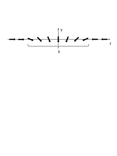
Figure 1: A schematic view of the magnetization orientation in the wire. $\lambda$ is the length of the domain wall.

In order to be able to linearize the system our first step must be to remove the spatially dependent, and in principle perhaps very large, magnetization. This is achievable by rotating the spin direction around the $x$-axis to a collinear ferromagnetic alignment via the following gauge transformation:Tatara and Fukuyama (1997); Korenman et al. (1977) $\mathbf{H}=\mathbf{U}^{\dagger}(z)\tilde{\mathbf{H}}\mathbf{U}(z)$, $\psi_{\sigma}(z)=U^{\dagger}_{\sigma\sigma^{\prime}}(z)\tilde{\psi}_{\sigma^{\prime}}(z)$, and $\mathbf{U}(z)=e^{\frac{i}{2}\Theta(z)\bm{\sigma}^{x}}$. The interaction is left unaffected as it is $SU(2)$ invariant, the magnetization is locally rotated to a Zeeman term $\tilde{H}_{M}\to H_{M}$, and a gauge potential is introduced: $\tilde{H}_{0}\to H_{0}+H_{G}$. Thus $H=H_{0}+H_{G}+H_{I}+H_{M}$ and

$$H_{0} = \sum_{\sigma}\int\,\mathrm{d}z\,\psi^{\dagger}_{\sigma}(z)\bigg{[}-\frac{1}{2m}\partial^{2}_{z}-\mu\bigg{]}\psi_{\sigma}(z),$$

$$H_{G} = \frac{1}{8m}\sum_{\sigma\sigma^{\prime}}\int\,\mathrm{d}z\psi^{\dagger}_{\sigma}(z)[\Theta^{\prime}(z)]^{2}\delta_{\sigma\sigma^{\prime}}\psi_{\sigma^{\prime}}(z)$$

$$-\frac{1}{4m}\sum_{\sigma\sigma^{\prime}}\int\,\mathrm{d}z\bigg{[}\psi^{\dagger}_{\sigma}(z)i\Theta^{\prime}(z)\sigma^{x}_{\sigma\sigma^{\prime}}\partial_{z}\psi_{\sigma^{\prime}}(z)$$

$$\qquad\qquad-\big{(}\partial_{z}\psi^{\dagger}_{\sigma}(z)\big{)}i\Theta^{\prime}(z)\sigma^{x}_{\sigma\sigma^{\prime}}\psi_{\sigma^{\prime}}(z)\bigg{]},$$

$$H_{M} = -\frac{J}{2}\sum_{\sigma}\int\,\mathrm{d}z\,\psi^{\dagger}_{\sigma}(z)\sigma^{z}_{\sigma\sigma}\psi_{\sigma}(z)$$ (2)

with $\Theta^{\prime}(z)=[\lambda\cosh(z/\lambda)]^{-1}$. The gauge potential has been written in a manifestly Hermitian form. The first term of $H_{G}$ is a pure potential scatterer, the next two terms describe spin-flip scattering. Without $H_{G}$ this is simply a spin split band model,Penc and Sólyom (1993) see Fig. 2. In our model the gauge potential introduces extended scattering terms, active over the length of the domain wall, which have to be included and are important for the low energy physics. The amplitudes of the spin-flip scattering and the potential term are proportional to $\lambda/\lambda_{F}$ and $(\lambda/\lambda_{F})^{2}$, respectively, where $\lambda_{F}$ is the Fermi wave length. We are here mainly interested in the case $\lambda\gg\lambda_{F}$. Except for very low temperatures the potential scattering term can then be safely neglected. On the other hand, in the limit of a sharp domain wall $\lambda\to 0$, then $\Theta^{\prime}(z)\to\pi\delta(z)$, the scattering terms become boundary operators, and both the spin-flip and the potential scatterer have to be taken into account. We will discuss these issues in greater depth in section III.

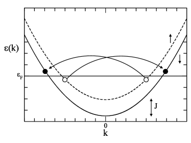
Figure 2: A schematic view of the spin split bands. One of the $g_{1\perp}$ processes is shown, which involve spin-flip scattering between left and right moving electrons.

The Hamiltonian (2) is now amenable to the usual bosonization procedure,Giamarchi (2003) the first step of which is linearization via the ansatz $\psi_{\sigma}(z)=e^{ik_{F\sigma}z}\psi_{\sigma+}(z)+e^{-ik_{F\sigma}z}\psi_{\sigma-}(z)$, where $k_{F\sigma}=\sqrt{2m(\mu\pm J/2)}$. The $+$ and $-$ indices denote the right- and left-moving electrons, respectively. Note that if the Zeeman term is large we must linearize around the spin split Fermi points, leading to the breakdown of spin-charge separation. After linearization we have $H_{0}+H_{M}\to H_{0\uparrow}+H_{0\downarrow}$, with the linearized Hamiltonians

$$H_{0\sigma}=v_{F\sigma}\!\!\!\int\!\!\,\mathrm{d}z[\psi^{\dagger}_{\sigma-}(z)i\partial_{z}\psi_{\sigma-}(z)-\psi^{\dagger}_{\sigma+}(z)i\partial_{z}\psi_{\sigma+}(z)]$$ (3)

where $mv_{F\sigma}=k_{F\sigma}$.

The interaction $H_{I}$ can be decomposed into spin parallel and spin perpendicular components and written as

$$\tilde{H}_{2} = \sum_{\sigma,r=\pm}\int\,\mathrm{d}z\bigg{[}\frac{\tilde{g}_{2\parallel\sigma}}{2}\rho_{\sigma r}\rho_{\sigma-r}+\frac{g_{2\perp}}{2}\rho_{\sigma r}\rho_{\bar{\sigma}-r}\bigg{]},$$ (4)

$$H_{4} = \sum_{\sigma,r=\pm}\int\,\mathrm{d}z\bigg{[}\frac{g_{4\parallel\sigma}}{2}\rho_{\sigma r}\rho_{\sigma r}+\frac{g_{4\perp}}{2}\rho_{\sigma r}\rho_{\bar{\sigma}r}\bigg{]}\textrm{, and}$$

$$H_{1} = \sum_{\sigma,r=\pm}\int\,\mathrm{d}z\bigg{[}-\frac{g_{1\parallel\sigma}}{2}\rho_{\sigma r}\rho_{\sigma-r}$$

$$+\frac{g_{1\perp\sigma}}{2}e^{2iz(k_{F\bar{\sigma}}-k_{F\sigma})}\psi^{\dagger}_{\sigma r}\psi^{\dagger}_{\bar{\sigma}-r}\psi_{\bar{\sigma}r}\psi_{\sigma-r}\bigg{]}.$$

Here we have suppressed the spatial indices and defined the local density $\rho_{\sigma\pm}=\psi^{\dagger}_{\sigma\pm}\psi_{\sigma\pm}$. Note that the “g-ology” given here refers to the already rotated model, not the original physical picture. The chiral electrons of this linearized model, physically speaking, have a non-collinear spin orientation throughout the wire. Umklapp processes scattering two left movers into right movers and vice versa are always neglected here due to the non-commensurate nature of the Fermi wavevectors. We can rescale the $g_{2\parallel\sigma}$ term to include the $g_{1\parallel\sigma}$ process by redefining $g_{2\parallel\sigma}=\tilde{g}_{2\parallel\sigma}-g_{1\parallel\sigma}$ with $\tilde{H}_{2}\to H_{2}$. The final $g_{1\perp\sigma}$ process, schematically shown in Fig. 2, can not be formulated as a density-density interaction.

Finally we have our model to be bosonized. We introduce the chiral bosonic fields $\phi_{\sigma r}(z)$.Giamarchi (2003) The vertex operator is

$$\psi_{\sigma r}(z)=\frac{1}{\sqrt{2\pi\alpha}}e^{ir\sqrt{2\pi}\phi_{\sigma r}(z)}$$ (5)

where $\alpha$ is a short distance cutoff. This leads to the following expression for the densities:

$$\rho_{\sigma r}(z)=-\frac{1}{\sqrt{2\pi}}\partial_{z}\phi_{\sigma r}.$$ (6)

Thus we can write the quadratic part of the bosonic Hamiltonian, $H_{q}$, which is composed from $H_{0}$, $H_{M}$, $H_{2}$, $H_{4}$ as a matrix equation

$$H_{q} = \int\,\mathrm{d}z[\partial_{z}\Phi(z)]^{T}\mathbf{M}\partial_{z}\Phi(z).$$ (7)

$[\Phi(z)]^{T}=(\phi_{\uparrow+},\phi_{\uparrow-},\phi_{\downarrow+},\phi_{\downarrow-})$. The bosonization procedure is thus sufficient to re-express all but $H_{1\perp}$ and $H_{G}$ in terms of a diagonalizable quadratic bosonic Hamiltonian. The matrix, $\mathbf{M}$, is

$$\mathbf{M} = \frac{1}{8\pi}\begin{pmatrix}4\pi v_{F\uparrow}+2g_{4\parallel\uparrow}&g_{2\parallel\uparrow}&g_{4\perp}&g_{2\perp}\\ g_{2\parallel\uparrow}&4\pi v_{F\uparrow}+2g_{4\parallel\uparrow}&g_{2\perp}&g_{4\perp}\\ g_{4\perp}&g_{2\perp}&4\pi v_{F\downarrow}+2g_{4\parallel\downarrow}&g_{2\parallel\downarrow}\\ g_{2\perp}&g_{4\perp}&g_{2\parallel\downarrow}&4\pi v_{F\downarrow}+2g_{4\parallel\downarrow}\end{pmatrix}.$$

$\mathbf{M}$ is a real symmetric matrix and as such has real eigenvalues. We can now diagonalize $\mathbf{M}$ and will do so in several steps to fully show the comparison with more standard expressions. In order for our final normal modes to have positive velocities there is a condition on this diagonalization procedure, given in the appendix. However, for any realistic microscopic model this condition should always be met, which can be shown explicitly in the case of the Hubbard model in a magnetic field.Penc and Sólyom (1993)

We can now make two unitary transformations. The first is $\phi_{\sigma\pm}=(\phi_{\sigma}\mp\theta_{\sigma})/\sqrt{2}$. Note that $\theta_{\sigma}$ is the adjoint of $\phi_{\sigma}$ and they satisfy $[\phi_{\sigma}(z),\Pi_{\sigma}(z^{\prime})]=i\delta(z-z^{\prime})$ where $\Pi_{\sigma}(z)=\partial_{z}\theta_{\sigma}(z)$. This first rotation has the effect of uncoupling the two adjoint fields. The second transformation is to rotate to the spin-charge representation: $\phi_{c/s}(z)=[\phi_{\uparrow}(z)\pm\phi_{\downarrow}(z)]/\sqrt{2}$ (and similar for the $\theta(z)$ fields). The effect of these two rotations can be summarized as $\tilde{\mathbf{M}}=\tilde{\mathcal{U}}^{-1}\mathcal{U}^{-1}\mathbf{M}\mathcal{U}\tilde{\mathcal{U}}$ with $[\tilde{\Phi}(z)]^{T}=[\Phi(z)]^{T}\mathcal{U}\tilde{\mathcal{U}}$ (see equations (32) and (33) in the appendix). If $[\tilde{\Phi}(z)]^{T}=(\phi_{s},\phi_{c},\theta_{s},\theta_{c})$ then our rotated Hamiltonian is defined by the matrix

$$\tilde{\mathbf{M}} = \frac{1}{2}\begin{pmatrix}\frac{v_{s}}{K_{s}}&v_{b}&0&0\\ v_{b}&\frac{v_{c}}{K_{c}}&0&0\\ 0&0&v_{s}K_{s}&v_{a}\\ 0&0&v_{a}&v_{c}K_{c}\end{pmatrix}.$$ (8)

Here $K_{s}$ and $K_{c}$ are the spin and charge Luttinger parameters, $v_{s}$ and $v_{c}$ are the spin and charge velocities, and $v_{a}$ and $v_{b}$ describe the coupling between the spin and charge sectors. These parameters are functions of the interaction strengths and Fermi velocities, and to lowest order can be calculated directly, see Eq. (30) in the appendix. At the non interacting $SU(2)$ symmetric point $K_{s}=K_{c}=1$. In the case of spin degeneracy we find, as expected, $v_{a}=v_{b}=0$ and the spin and charge modes decouple.

The non-quadratic contributions from $H_{G}$ in this representation are

$$H^{f}_{Gsf} = \frac{g_{f}}{2\pi m\alpha}\int\,\mathrm{d}z\Theta^{\prime}(z)\sin[\sqrt{2\pi}\theta_{s}(z)]$$

$$\sin[z(k_{F\uparrow}-k_{F\downarrow})+\sqrt{2\pi}\phi_{s}(z)],$$

$$H^{b}_{Gsf} = \frac{g_{b}}{2\pi m\alpha}\int\,\mathrm{d}z\Theta^{\prime}(z)\sin[\sqrt{2\pi}\theta_{s}(z)]$$

$$\sin[-z(k_{F\uparrow}+k_{F\downarrow})+\sqrt{2\pi}\phi_{c}(z)],$$

$$H^{f}_{Gp} = -\frac{1}{8m}\sqrt{\frac{2}{\pi}}\int\,\mathrm{d}z[\Theta^{\prime}(z)]^{2}\partial_{z}\phi_{c}(z),\textrm{ and}$$

$$H^{b}_{Gp} = -\frac{1}{8\pi m}\sum_{\sigma}\int\,\mathrm{d}zg_{b\sigma}[\Theta^{\prime}(z)]^{2}$$

$$\cos[2zk_{F\sigma}+2\sqrt{\pi}\phi_{\sigma}(z)].$$

The first term, $H^{f}_{Gsf}$, describes a forward scattering (upper index “f”) spin-flip (lower index “sf”) process where a fermion is exchanged between the spin up and spin down bands but stays on the same side of the Fermi surface. The second term, $H^{b}_{Gsf}$, is a backward scattering spin-flip term where a fermion is exchanged between the bands and also moves from one side of the Fermi surface to the other. The third contribution $H^{f}_{Gp}$ is a potential (lower index “p”), spin conserving forward scattering process. The final term, $H^{b}_{Gp}$, is a spin conserving backward scattering process. This is the scatterer considered by Kane and Fisher which gives rise to the usual insulating fixed point.Kane and Fisher (1992b) All scattering processes are only active over the length of the domain wall (or, more generally speaking, the region of non-collinear spin order) where $\Theta^{\prime}(z)\neq 0$. The scattering coupling constants for forward and backward spin-flip scattering from the domain wall are given by $g_{f/b}=k_{F\uparrow}\pm k_{F\downarrow}$. We have also introduced the bare potential scattering values $g_{b\sigma}=1/\alpha$ for convenience.

The non-quadratic interaction term $H_{1\perp}$ is then

$$H_{1\perp} = \frac{2}{(2\pi\alpha)^{2}}\int\,\mathrm{d}z\cos[2\sqrt{2\pi}\phi_{s}(z)]$$

$$\big{[}g_{1\perp\uparrow}e^{-2iz(k_{F\uparrow}-k_{F\downarrow})}+g_{1\perp\downarrow}e^{2iz(k_{F\uparrow}-k_{F\downarrow})}\big{]}.$$

This last term also corresponds to a backward scattering process. It stems, however, from the interaction $H_{I}$ and therefore involves two fermions being scattered between the different bands and from one side of the Fermi surface to the other. These contributions have their simplest interpretation in terms of the spin and charge modes. However, the spin and charge modes are not eigenmodes of the model, see Eq. (8), and we also require Eqs. (II) and (II) in the appropriately rotated basis.

The diagonalization of $\tilde{\mathbf{M}}$ introduces new velocities, $u_{i}$, for $H_{q}$ and a set of $\{T_{i}^{\theta,\phi}\}$ parameters. It can be summarized as

$$\begin{pmatrix}\phi_{c}(z)\\ \phi_{s}(z)\end{pmatrix} = \begin{pmatrix}\tilde{T}^{\phi}_{1}&\tilde{T}^{\phi}_{2}\\ T^{\phi}_{1}&T^{\phi}_{2}\end{pmatrix}\begin{pmatrix}\phi_{1}(z)\\ \phi_{2}(z)\end{pmatrix}\textrm{ and}$$

$$\begin{pmatrix}\theta_{c}(z)\\ \theta_{s}(z)\end{pmatrix} = \begin{pmatrix}\tilde{T}^{\theta}_{1}&\tilde{T}^{\theta}_{2}\\ T^{\theta}_{1}&T^{\theta}_{2}\end{pmatrix}\begin{pmatrix}\theta_{1}(z)\\ \theta_{2}(z)\end{pmatrix}$$ (11)

with the parameters $\{T_{i}^{\theta,\phi}\}$ as given in Eq. (A) of the appendix. They are all known in terms of the previously mentioned Luttinger parameters. We have also simultaneously rescaled the fields to obtain two distinct eigenvalues rather than four. The final Hamiltonian is $H=H_{q}+H_{1\perp}+H^{f}_{Gsf}+H^{b}_{Gsf}+H^{b}_{Gp}+H^{f}_{Gp}$ where

$$H_{q} = \frac{u_{i}}{2}\int\,\mathrm{d}z\,\left[(\partial_{z}\phi_{i}(z))^{2}+(\Pi_{i}(z))^{2}\right]$$ (12)

and, with summation over $i$ and $j$ implied:

$$H^{f}_{Gsf} = \frac{g_{f}}{2\pi m\alpha}\int\,\mathrm{d}z\,\Theta^{\prime}(z)\sin[\sqrt{2\pi}T_{i}^{\theta}\theta_{i}(z)]$$

$$\sin[z(k_{F\uparrow}-k_{F\downarrow})+\sqrt{2\pi}T_{j}^{\phi}\phi_{j}(z)],$$

$$H^{b}_{Gsf} = \frac{g_{b}}{2\pi m\alpha}\int\,\mathrm{d}z\,\Theta^{\prime}(z)\sin[\sqrt{2\pi}T_{i}^{\theta}\theta_{i}(z)]$$

$$\sin[-z(k_{F\uparrow}+k_{F\downarrow})+\sqrt{2\pi}\tilde{T}_{j}^{\phi}\phi_{j}(z)],$$

$$H^{f}_{Gp} = -\frac{1}{8m}\sqrt{\frac{2}{\pi}}\int\,\mathrm{d}z[\Theta^{\prime}(z)]^{2}\tilde{T}^{\phi}_{i}\partial_{z}\phi_{i}(z),\textrm{ and}$$

$$H^{b}_{Gp} = -\frac{1}{8\pi m}\sum_{\sigma}\int\,\mathrm{d}zg_{b\sigma}[\Theta^{\prime}(z)]^{2}$$

$$\cos[2zk_{F\sigma}+\sqrt{2\pi}(\tilde{T}^{\phi}_{i}+\sigma_{\sigma\sigma}^{z}T^{\phi}_{i})\phi_{i}(z)]$$

for the scattering terms and finally:

$$H_{1\perp} = \frac{2}{(2\pi\alpha)^{2}}\int\,\mathrm{d}z\cos[2\sqrt{2\pi}T_{i}^{\phi}\phi_{i}(z)]$$

$$\big{[}g_{1\perp\uparrow}e^{-2iz(k_{F\uparrow}-k_{F\downarrow})}+g_{1\perp\downarrow}e^{2iz(k_{F\uparrow}-k_{F\downarrow})}\big{]}.$$

The appropriate excitations of such an $SU(2)$ asymmetric model have no obvious physical interpretation. This effective bosonic field theory lays the foundation of our further analysis. A similar model is found by Braunecker et al.Braunecker et al. (2009a, b) in a different situation, and of course by Pereira and MirandaPereira and Miranda (2004) but without the $H^{f}_{Gsf}$ and $H_{1\perp}$ terms which do not play any role for very sharp domain walls where the length scale $\lambda$ is no longer present. However they also neglect $H^{b}_{Gp}$ which does play a role in the sharp wall limit. Indeed it is this term which, when dominant, leads to the Kane and Fisher insulating fixed point. This will become clear in Sec. III where the case of a sharp domain wall is obtained as a specific limit in our general analysis.

III Low Energy Physics

In the generic case, we have three natural length scales present in the problem: $\lambda_{+}\sim(k_{F\uparrow}+k_{F\downarrow})^{-1}$ related to spin-flip backward scattering, $\lambda_{-}\sim(k_{F\uparrow}-k_{F\downarrow})^{-1}$ related to spin-flip forward scattering, and the domain wall length $\lambda$. In the limit of weak magnetization $\lambda_{-}\to\infty$ and $2\lambda_{+}\to\lambda_{F}$ while, on the other hand, the limit of large magnetization, when one spin channel becomes frozen out, gives $\lambda_{+}\approx\lambda_{-}\approx\lambda_{F}$. It is crucial for the further analysis to observe that the relative importance of the forward and backward scattering terms is now not only determined by their scaling dimensions but also by the hierarchy of the three different length scales. Furthermore, in the RG flow we must distinguish between the extended and sharp regimes. In the beginning of the RG flow we have an extended domain wall and the scattering terms can be treated as bulk terms of dimension $d=2$. However, when the ultraviolet momentum cutoff $\Lambda$ during the RG process becomes of the order $1/\lambda$ then the extended domain wall will begin to look effectively point like, i.e. of dimension $d=1$. The scattering terms then become boundary operators. At this stage the direction and rate of the flow of all of the operators can change, leading to the final low-temperature fixed points. For this effective $d=1$ flow we must take the result of the $d=2$ flow as the “zeroth order” coupling constants. In physical terms, the domain wall starts to look point-like if the electrons are correlated spatially over lengths much larger than the domain wall length, i.e., if $J/T\gg\lambda/\alpha$.

Another important point to note is that for an extended domain wall we usually have $\lambda\gg\lambda_{+}$, i.e., the backward scattering terms are strongly oscillating over the length of the domain wall. This leads to very small bare effective backward scattering couplings which can be estimated as follows: The derivative of the domain wall profile, $\Theta^{\prime}(z)$, can be Fourier transformed leading to $\Theta^{\prime}(k)=\pi/\cosh(\pi k\lambda/2)$. The non-oscillating component of the backward scattering amplitude is then proportional to $g_{b}\Theta^{\prime}(k=\pm 1/\lambda_{+})$. Since $\Theta^{\prime}(k)$ is a function which is sharply peaked at $k=0$ for long domain walls, we have $|g_{b}\Theta^{\prime}(k=\pm 1/\lambda_{+})|\sim|g_{b}\exp(-\lambda/\lambda_{+})|\ll 1$. If backward scattering is relevant, then the effective coupling constant will grow under the RG flow as

$$g_{b}^{\rm eff}\sim g_{b}\exp(-\lambda/\lambda_{+})\left(\frac{T_{0}}{T}\right)^{d-\gamma_{b}}$$ (14)

where $T_{0}$ is an energy scale of order $J$. Backward scattering will only have an appreciable effect if the initially small bare coupling has again become of order $1$ under the RG flow. This requires temperatures $T/J<\exp(-\lambda/\lambda_{+})$ which are extremely small for many realistic situations. We therefore expect that forward scattering—ignored in previous investigations of the domain wall problem—will play the dominant role in these cases.

Before discussing the various regimes any further, we want to derive the first order RG equations for the forward and backward scattering terms. We start by writing a functional integral partition functionNegele and Orland (1998)

$$\mathcal{Z}=\int D\phi_{i}D\Pi_{i}e^{-\int_{0}^{\beta}\,\mathrm{d}\tau\big{[}\int\,\mathrm{d}z[-i\Pi_{i}(z)\partial_{\tau}\phi_{i}(z)]+H[\Pi_{i}(z),\phi_{i}(z)]\big{]}}$$ (15)

with periodic boundary conditions in imaginary time $\tau$. Following the standard procedure we split the fields into fast, $\phi^{>}$, and slow, $\phi^{<}$, fields. Our fast fields are defined for $\Lambda^{\prime}<|k|,|\omega|/u_{i}<\Lambda$, and the slow for $|k|,|\omega|/u_{i}<\Lambda^{\prime}$, with $\Lambda$ an ultraviolet cut-off. Expanding the exponent in terms of $H_{1\perp}$, $H^{f,b}_{Gsf}$ and $H^{b}_{Gp}$ and performing the averaging over the fast modes we then re-exponentiate the expression to find the appropriate scaling equations. The flow is parametrized in terms of $l$, defined as $\Lambda=\Lambda_{0}e^{-l}$ and $\Lambda^{\prime}=\Lambda_{0}e^{-l-\delta l}$.

We find for the $H_{1\perp}$ term to first order that

$$\frac{\,\mathrm{d}g_{1\perp\sigma}}{\,\mathrm{d}l}=g_{1\perp\sigma}\big{[}2-\underbrace{2[(T^{\phi}_{1})^{2}+(T^{\phi}_{2})^{2}]}_{\equiv\gamma_{1}}\big{]}.$$ (16)

This term is an irrelevant perturbation ($\gamma_{1}>2$) for any realistic situation we are here interested in. In the limit of weak magnetization we can simplify the expression to find $\gamma_{1}=2K_{s}$. In this limit $K_{s}>1$ and it becomes clear that the term is irrelevant.

The same analysis is performed on the domain wall scattering terms. For spin-flip back scattering we find:

$$\frac{\,\mathrm{d}g_{b}}{\,\mathrm{d}l}=g_{b}\big{[}d-\underbrace{\frac{1}{2}[(\tilde{T}^{\phi}_{1})^{2}+(\tilde{T}^{\phi}_{2})^{2}+(T^{\theta}_{1})^{2}+(T^{\theta}_{2})^{2}]}_{\equiv\gamma_{b}}\big{]}.$$ (17)

As already mentioned $d$ is the dimension of the wall, for spatially extended walls this is $2$, whereas it is $1$ in the limit of an infinitely sharp wall. As usual the perturbation is relevant (irrelevant) if $\gamma_{b}<d$ ($\gamma_{b}>d$). In the limit of $J\to 0$ we can simplify this expression to $\gamma_{b}=[(K_{s})^{-1}+K_{c}]/2$ consistent with Refs. Pereira and Miranda, 2004, Pereira, 2004. If we consider the Luttinger parameters for the Hubbard model in the zero magnetization limit we see that this term is always relevant for repulsive interactions both for $d=1$ and $d=2$ but can also become irrelevant in both cases for attractive interactions. In the general case described by Eq. (17) the relevance or irrelevance of backward scattering depends on the set of rotation parameters $T_{i}^{\theta,\phi}$ and no general conclusions are possible.

Similarly the spin-flip forward scattering equation stands as

$$\frac{\,\mathrm{d}g_{f}}{\,\mathrm{d}l}=g_{f}\big{[}d-\underbrace{\frac{1}{2}[(T^{\phi}_{1})^{2}+(T^{\phi}_{2})^{2}+(T^{\theta}_{1})^{2}+(T^{\theta}_{2})^{2}]}_{\equiv\gamma_{f}}\big{]}.$$ (18)

In the limit of $J\to 0$ this simplifies to $\gamma_{f}=[(K_{s})^{-1}+K_{s}]/2$. Since $K_{s}\geq 1$, in this limit it follows that $\gamma_{f}\geq 1$. For the case of a sharp wall ($d=1$) forward scattering is therefore always irrelevant.Pereira and Miranda (2004); Pereira (2004) In the case of an extended wall ($d=2$), on the other hand, forward scattering is relevant in this limit if $K_{s}<2+\sqrt{3}$. The generic case described by Eq. (18) is again very complicated to analyze. However, at least for simple microscopic models and in the limit of weak interactions where the rotation parameters can be calculated explicitly (see Eqs. (36), (37) in the appendix), we find that forward scattering is always relevant for $d=2$.

The potential back scattering equations are, for the two spin channels,

$$\frac{\,\mathrm{d}g_{b\sigma}}{\,\mathrm{d}l}=g_{b\sigma}\big{[}d-\underbrace{\frac{1}{2}[(\tilde{T}^{\phi}_{1}\pm T^{\phi}_{1})^{2}+(\tilde{T}^{\phi}_{2}\pm T^{\phi}_{2})^{2}]}_{\equiv\gamma_{b\sigma}}\big{]}$$ (19)

with the plus (minus) sign applying for $\sigma=\uparrow$ ($\sigma=\downarrow$). In the limit of $J\to 0$ we find $\gamma_{b\sigma}=[K_{c}+K_{s}]/2$. In the isotropic limit, $K_{s}\to 1$, this term is always relevant for repulsive interactions. In general however it can be either relevant or irrelevant. Indeed, it is also possible that potential backward scattering is relevant for one spin channel and irrelevant for the other.

The potential forward scattering term has scaling dimension $x=1$. It will therefore be relevant for an extended domain wall and marginal in the limit of a sharp wall.

As an example, we present in Fig. 3 the two scaling dimensions for forward and backward spin-flip scattering off an extended wall as a function of $\xi=J/2\varepsilon_{F}$ calculated for a $U$-$V$ model with an on-site interaction $U/t=1.10$, and nearest neighbor interaction $V/t=0.11$, where $t$ is the hopping amplitude. Here the parameters of our low-energy effective model are determined in a lowest order expansion in the interaction parameters.

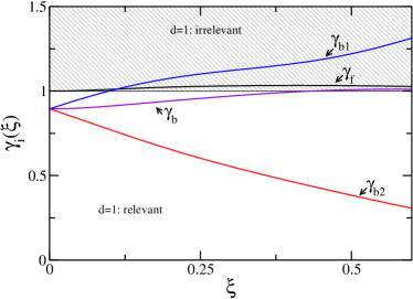
Figure 3: (Color online) $\gamma_{f,b}$ and $\gamma_{b\sigma}$ for forward and backward, spin flip and potential, scattering from an extended domain wall obtained for a specific $U$-$V$ model (see text for details) as a function of $\xi=J/2\varepsilon_{F}$. The regions where the operators are relevant or irrelevant for $d=1$ are marked. The condition $K_{s}=1$ has been imposed by hand at the $SU(2)$ symmetric point ($J=0$), see appendix.

We want to remind the reader that by rotating back to the original physical model one finds that “spin-flip forward scattering” refers to an electron which passes through the wall without changing its spin.

III.1 RG flow in the extended domain wall regime

At first we will focus on the $d=2$ case. For extended domain walls ($\lambda\gg\lambda_{F}$) the bare potential scattering terms $\sim(\lambda/\lambda_{F})^{2}$ are much smaller than the spin-flip scattering terms $\sim(\lambda/\lambda_{F})$. In the temperature range where it is appropriate to use the RG flow with $d=2$ we can therefore neglect the potential scattering terms. They will, however, become important for the RG flow with $d=1$ at even lower temperatures discussed in the next subsection.

Though with the physical parameters we consider in section IV we find both $g_{f,b}$ to be relevant, by varying the $v_{c,s}$, $K_{c,s}$, and $v_{a,b}$ parameters we can find regimes where forward scattering remains relevant but backscattering becomes irrelevant.

We can now identify several regimes. We focus here first on the small magnetization limit close to half-filling where $\lambda_{-}\gg\lambda_{+}$. For the backward scattering Hamiltonian, $H_{Gsf}^{b}$, Eq. (II), this means that we take the limit where $k_{F\uparrow}\approx k_{F\downarrow}\to k_{F}\approx\pi/2$. We can then simplify (II) and find

$$H_{Gsf}^{b} = \frac{g_{b}}{2\pi m\alpha}\int\,\mathrm{d}z\Theta^{\prime}(z)\sin[\sqrt{2\pi}\theta_{s}(z)]$$ (20)

$$\cos[2zk_{F}]\sin[\sqrt{2\pi}\phi_{c}(z)].$$

We now consider the case that this term is relevant, i.e., $g_{b}$ becomes large at low temperatures. Firstly, for ‘narrow enough’ walls, i.e., for domain walls of the order of the Fermi wave length $\lambda_{F}$ when the $2k_{F}$ oscillations do not cancel out the contributions, then in order to minimize the energy the fields become locked over the length of the domain wall in the values $\{\phi_{c}=\sqrt{2\pi}(m+\frac{3}{4}),\theta_{s}=\sqrt{2\pi}(n+\frac{1}{4})\}$ or $\{\phi_{c}=\sqrt{2\pi}(m+\frac{1}{4}),\theta_{s}=\sqrt{2\pi}(n+\frac{3}{4})\}$ for integer $m,n$. Therefore the domain wall becomes an impenetrable barrier for both charge and spin excitations and we find a spin charge insulator.Pereira and Miranda (2004); Fabrizio and Gogolin (1995) If we consider longer domain walls then, as already discussed previously, the effective bare coupling for backward scattering will be close to zero. Hence, for extended domain walls, $\lambda\gg\lambda_{F}$, forward scattering is always the more important because $\lambda_{+}\ll\lambda_{-}$.

Therefore there is also a regime in which only forward scattering is relevant: either the long domain wall case or the case of irrelevant backward scattering ($\gamma_{b}>2$). Considering again the limit of small magnetization and a system close to half-filling, the forward scattering term in Eq. (II) simplifies to

$$H_{Gsf}^{f} = \frac{g_{f}}{2\pi m\alpha}\int\,\mathrm{d}z\Theta^{\prime}(z)\sin[\sqrt{2\pi}\theta_{s}(z)]$$ (21)

$$\cos[z(k_{F\uparrow}-k_{F\downarrow})]\sin[\sqrt{2\pi}\phi_{s}(z)].$$

In order to minimize the energy in this case the fields become locked over the length of the domain wall in the values $\{\phi_{s}=\sqrt{2\pi}(m+\frac{3}{4}),\theta_{s}=\sqrt{2\pi}(n+\frac{1}{4})\}$ or $\{\phi_{s}=\sqrt{2\pi}(m+\frac{1}{4}),\theta_{s}=\sqrt{2\pi}(n+\frac{3}{4})\}$ for integer $m,n$. In this scenario only the spin sector is frozen out and we find a C$1$S$0$ phase where the spin mode is gapped but charge excitations remain gapless.Balents and Fisher (1996) In the physical reference frame this is a state in which the incoming spin current does not scatter from the domain wall and, after traversing the domain wall, ends in the anti-parallel spin configuration with respect to the bulk. This means that the domain wall profile can no longer be taken as adiabatic.

From the above considerations we have several possibilities. Firstly we can have backward scattering as either relevant or irrelevant. Secondly we must consider the relative length scales. If $\lambda_{+}<\lambda$ then the backward scattering terms are small due to averaging over their oscillations. A similar case holds for the forward scattering with $\lambda_{+}\to\lambda_{-}$ in the preceding. For the case in which both the forward and backward scattering length-scales are shorter than the domain wall length we end up in the completely adiabatic limit, as one would expect, and the system shows Luttinger liquid properties (“adiabatic LL”). Again we note that at extremely low temperatures we have to switch to a $d=1$ RG flow and backward scattering processes will begin to dominate and can lead to insulating regimes. In principle, we can also be in the opposite regime when both forward and backward scattering length-scales are longer than the domain wall length in which case the scaling dimensions of the forward and backward scattering terms alone determine what the low-energy fixed point is. Note that this is possible without requiring a very sharp delta function like domain wall profile. In general, however, the low-temperature phase the system ends up in in the extended regime depends not only on the relevance of the operators, but also on the hierarchy of length scales.

The different behaviour in the extended regime which could be identified from the first order RG equations are summarized in table 1.

Table 1: The different phases of the ferromagnetic Luttinger liquid with an extended domain wall ($d=2$, relevant spin-flip forward scattering) depending on the scaling dimensions of the spin-flip backward scattering operator and the hierarchy of the three length scales present in the problem.

	$\lambda\lesssim\lambda_{\pm}$	$\lambda_{+}<\lambda<\lambda_{-}$	$\lambda_{\pm}<\lambda$
$2-\gamma_{b}>0$	Spin and charge	C$1$S$0$	Adiabatic
	insulator		LL
$2-\gamma_{b}<0$	C$1$S$0$	C$1$S$0$	Adiabatic
			LL

Finally, let us also comment on the case of a generic magnetization and arbitrary filling. In this case the analysis above stays valid, the spin and charge modes, however, get locked into more complicated spin and charge density wave states over the length of the domain wall.

III.2 Fixed points of the $d=1$ sharp domain wall regime

For the case of a very sharp domain wall ($d=1$) we have shown that forward spin-flip scattering is always irrelevant. The forward potential scattering term is marginal and we will ignore it as well. In this case the possible phases are therefore determined by the scaling dimensions of the two backward scattering terms alone. (Naturally for a sharp wall the length-scales can play no further role.) Formally one can find the sharp domain wall limit from Eq. (2) by taking the limit $\lambda\to 0$, which requires $\Theta^{\prime}(z)\to\pi\delta(z)$. This leads to an effective model where all the boundary scattering terms allowed by symmetry are present. A full description of the phase space for this model with different relevant perturbations present requires the solution to the second order RG equations to find the separatrix between the different low temperature fixed points. The second order equation for our model is more complicated than for the standard sine-Gordon model. A diagonal equation in the $\phi_{i}$’s is not recovered and to perform any further analysis we would have to re-diagonalize the problem and then renormalize the model once again, repeating these steps until we reached the fixed point.Chudzinski et al. (2010) This is perhaps not totally unexpected as the scattering terms we are dealing with explicitly couple the normal modes. We leave the more involved second order RG analysis to a future work and focus here on what the first order equations can tell us. The flow of a similar model has already been analyzed by Araújo, et al.Araújo et al. (2006, 2007) using poor man’s scaling. In that work they consider both spin-flip and pure potential backscattering from a sharp domain wall, treating the interaction only perturbatively. They find phases dominated by the spin-flip and pure potential backscattering processes. In contrast Pereira and MirandaPereira and Miranda (2004) consider only the spin-flip backscattering term and hence cannot recover all possible low energy phases.

There are three possible fixed points of the RG flow depending on the relative relevance of the three backscattering channels, $g_{b}$, $g_{b\uparrow}$, and $g_{b\downarrow}$. The system can flow to a spin and charge insulator, an effectively spinless Luttinger liquid, or a spin-full Luttinger liquid. Furthermore the spin and charge insulator itself can show different physical behaviour in the region of the domain wall depending on the relative relevance of the backscattering operators. This behaviour will be confined to some region around the boundary. Firstly let us discuss the spin and charge insulating phase. If the pure potential backscattering for both spin channels is relevant and dominates, $\gamma_{b\sigma}<\gamma_{b}$, then the system will flow to the spin and charge insulating fixed point already studied by Kane and FisherKane and Fisher (1992b) with the spin part of the system remaining completely unaffected. If the spin-flip back scattering term is relevant and dominates, $\gamma_{b}<\gamma_{b\sigma}$, then we have the fixed point analyzed by Pereira and Miranda.Pereira and Miranda (2004) The spin-flip back scattering will tend to equilibriate the number of up and down spins. This fixed point must therefore correspond physically to a spin and charge insulator with a region of reduced spin polarization around the boundary. It is also possible to have the situation where $\gamma_{b\sigma}<\gamma_{b}<\gamma_{b\bar{\sigma}}$ with $\gamma_{b\sigma},\gamma_{b}<1$. In this case as the system approaches the fixed point first one spin channel will become insulating, however, before the second spin channel also becomes insulating the spin-flip backscattering term will tend to align the spins into the first channel. Once the spins are scattered into the first channel they are more likely to be scattered without a spin flip than back into the other spin channel. Therefore the final fixed point will likely be an insulator with a region of increased spin polarization around the domain wall. Secondly if potential back scattering is relevant for one channel but irrelevant for the other and spin-flip scattering is irrelevant as well, then we are left with an effective spinless Luttinger liquid, i.e., we have one insulating and one conducting channel. Finally, if all back scattering operators are irrelevant, then the system remains a Luttinger liquid.

These results are summarized in table 2.

Table 2: The different phases of the ferromagnetic Luttinger liquid with an effectively sharp domain wall ($d=1$, irrelevant forward scattering) depending on the relevance or irrelevance of the backward scattering operators. The physics of the system surrounding the domain wall for the spin and charge insulating phase depends upon the relative relevance of the backward scattering operators and is discussed fully in the text.

$\gamma_{b}<1$	$\gamma_{b\sigma}<1$	$\gamma_{b}>1$
and/or $\gamma_{b\uparrow},\gamma_{b\downarrow}<1$	$\gamma_{b},\gamma_{b\bar{\sigma}}>1$	$\gamma_{b\uparrow},\gamma_{b\downarrow}>1$
Spin and charge
insulator	Effective spinless LL	LL

IV Spin and Charge Density in the perturbative regime

We now return to the case of an extended domain wall, $\lambda\gg\lambda_{F}$, where the potential scattering terms can be ignored and consider a perturbative temperature regime where the spin flip scattering terms can be treated perturbatively. This allows us to calculate the spin and charge densities around the domain wall. Spin and charge density oscillations around impurities are not only experimentally relevant, but also provide a useful theoretical tool to analyze the dominant physical scattering processes in general low dimensional strongly correlated systems.Eggert and Rommer (1998); Anfuso and Eggert (2006); Eggert et al. (2007); Sirker and Laflorencie (2009) As we are interested in the case where both forward and backward scattering are relevant perturbations, a perturbative treatment of the scattering terms will break down at low enough temperatures. We indeed find that the perturbative corrections increase as a power law in inverse temperature. In order for perturbation theory to be valid, we find that the following conditions, for forward and backward scattering terms respectively, have to be held:

$$\left(\frac{T}{T^{*}_{1}}\right)^{\alpha_{1}}\left(\frac{T}{T^{*}_{2}}\right)^{\alpha_{2}} \ll \frac{4\pi\lambda mT}{g_{f}[T^{\phi}_{1}T^{\theta}_{1}+T^{\phi}_{2}T^{\theta}_{2}]}$$ (22)

and

$$\left(\frac{T}{T^{*}_{1}}\right)^{\beta_{1}}\left(\frac{T}{T^{*}_{2}}\right)^{\beta_{2}} \ll \frac{4\pi\lambda mT}{g_{b}[T^{\phi}_{1}T^{\theta}_{1}+T^{\phi}_{2}T^{\theta}_{2}]}.$$ (23)

Here $T^{*}_{i}\sim u_{i}/(2\pi\alpha)$ is a cutoff scale and the exponents are given by $\alpha_{i}=[(T^{\phi}_{i})^{2}+(T^{\theta}_{i})^{2}]/4$ and $\beta_{i}=[(\tilde{T}^{\phi}_{2})^{2}+(T^{\theta}_{2})^{2}]/4$. Note that $\alpha_{1}+\alpha_{2}=\gamma_{f}/2$ and $\beta_{1}+\beta_{2}=\gamma_{b}/2$ so that the scaling dimensions show up in Eqs. (22) and (23) in the expected way.

We want to present our results in the physical unrotated frame. The perturbative results are, however, obtained in the rotated frame so that we have to use the gauge transformation $\mathbf{U}(z)$ once more. The spin density, in the physical frame, is

$$\vec{S}(z)=\frac{1}{2}{\tilde{\bm{\psi}}}^{\dagger}(z)\vec{{\bm{\sigma}}}{\tilde{\bm{\psi}}}(z)=\frac{1}{2}{\bm{\psi}}^{\dagger}(z)\underbrace{{\bm{U}}^{\dagger}\vec{{\bm{\sigma}}}{\bm{U}}}_{\vec{{\bm{\sigma}}}^{\prime}}{\bm{\psi}}(z)$$ (24)

where the gauge rotated Pauli matrices are given explicitly by

$${\bm{\sigma}}^{\prime}_{x} = {\bm{\sigma}}^{x},$$

$${\bm{\sigma}}^{\prime}_{y} = \cos[\Theta(z)]{\bm{\sigma}}^{y}-\sin[\Theta(z)]{\bm{\sigma}}^{z},$$

$${\bm{\sigma}}^{\prime}_{z} = \sin[\Theta(z)]{\bm{\sigma}}^{y}+\cos[\Theta(z)]{\bm{\sigma}}^{z}.$$ (25)

Using these relations, the spin densities in the physical frame $\vec{S}(z)$ can now be constructed from the spin densities $\vec{S}_{0}(z)=\frac{1}{2}{\bm{\psi}}^{\dagger}(z)\vec{{\bm{\sigma}}}{\bm{\psi}}(z)$ in the rotated frame. The corrections to the bulk in first order in forward and backward scattering off the domain wall are given by

$$\langle\Delta S^{x}_{0}(z)\rangle = \frac{1}{\alpha\pi}\big{\langle}\cos[\sqrt{2\pi}\theta_{s}(z)]\times$$

$$\big{[}\cos[(k_{F\uparrow}-k_{F\downarrow})z+\sqrt{2\pi}\phi_{s}(z)]$$

$$+\cos[(k_{F\uparrow}+k_{F\downarrow})z+\sqrt{2\pi}\phi_{c}(z)]\big{]}\big{\rangle},$$

$$\langle\Delta S^{y}_{0}(z)\rangle = \frac{1}{\alpha\pi}\big{\langle}\sin[\sqrt{2\pi}\theta_{s}(z)]\times$$

$$\big{[}\cos[(k_{F\uparrow}-k_{F\downarrow})z+\sqrt{2\pi}\phi_{s}(z)]$$

$$+\cos[(k_{F\uparrow}+k_{F\downarrow})z+\sqrt{2\pi}\phi_{c}(z)]\big{]}\big{\rangle}\textrm{, and}$$

$$\langle\Delta S^{z}_{0}(z)\rangle = \bigg{\langle}-\frac{1}{\sqrt{2\pi}}\partial_{z}\phi_{s}(z)$$

$$+\frac{1}{2\alpha\pi}\sum_{\sigma}\sigma^{z}_{\sigma\sigma}\cos[2xk_{F\sigma}-2\sqrt{\pi}\phi_{\sigma}(z)]\bigg{\rangle}.$$

Note that in the linearization procedure, strictly speaking, we should write $\psi_{\sigma}(z)=\psi_{0\sigma}(z)+e^{ik_{F\sigma}z}\psi_{\sigma+}(z)+e^{-ik_{F\sigma}z}\psi_{-\sigma}(z)$. As such there are ${\bm{\psi}}_{0}^{\dagger}(z)\vec{{\bm{\sigma}}}{\bm{\psi}}_{0}(z)$ terms missing from the above spin densities which give the bulk values. We can also use a description where we absorb the effective magnetic field by a shift in the bosonic fields instead of linearizing around the spin split Fermi points. In this case, however, we must take into account curvature terms.Pereira et al. (2007) This would reintroduce the bulk spin density terms explicitly in Eqs. (IV) to (IV).

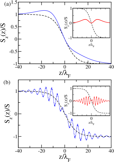
Figure 4: (Color online) The spin density $S_{z}(z)/S$, showing the zeroth order (dashed line) term and the total value (blue, solid line). The inset shows a comparison of the the zeroth order (dashed line) and first order (red, solid line) terms. Zeroth and first order refer to an expansion in the scattering potential. All the spin figures are normalized to the average value per conduction electron, $S=\frac{1}{2}$. The domain wall length is $\lambda=10\lambda_{F}$ with (a) $\frac{J}{2}=0.112$ eV and $T=25$K, and (b) $\frac{J}{2}=2.23$ eV and $T=50$K.

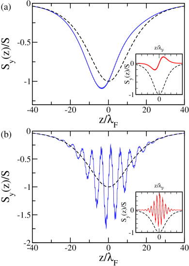
Figure 5: (Color online) Same as Fig. 4 but for the spin density $S_{y}(z)/S$.

In the following, we want to consider two examples. Example (a) corresponds to a case where $\lambda_{+}\ll\lambda<\lambda_{-}$ so that only forward scattering contributes. In example (b), on the other hand, we consider the case $\lambda_{+}\ll\lambda_{-}\lesssim\lambda$ so that forward scattering is again dominant but is oscillating over the length of the domain wall. More specifically, we consider values which are appropriate for Fe, $\lambda_{F}=0.367$ nm, and a lattice cutoff $\alpha=\lambda_{F}$. We plot results for two sets of parameters: (a) $\frac{J}{2}=0.112$ eV, $\lambda=10\lambda_{F}$, and $T=25$K; and (b) $\frac{J}{2}=2.23$ eV, $\lambda=10\lambda_{F}$, and $T=50$K. These parameters give us the following scaling terms: (a) $\gamma_{f}=1.12$, and $\gamma_{b}=0.923$; and (b) $\gamma_{f}=1.09$, and $\gamma_{b}=0.937$. In both cases the conditions (22) and (23) are fulfilled with the ratio of r.h.s divided by l.h.s being of the order $10^{-3}$ for the condition on backward scattering, Eq. (23), and of the order $10^{-1}$ for forward scattering, Eq. (22).

Figs. 4, and 5 show the spin density around the domain wall, normalized to the average value per conduction electron, $S=\frac{1}{2}$. For the situation where the length-scale of the forward scattering oscillations is larger than the domain wall length, case (a), the spin density profile is significantly altered, see Figs. 4(a), 5(a). Such a shift will affect how the domain wall itself behaves in the effective magnetic field applied by the conduction electrons and therefore will strongly affect the domain wall dynamics. As expected, the backward scattering plays no role in the considered temperature range.

The asymmetric distortion of the spin density clearly visible in Figs. 4(a) and 5(a) is due to the addition of antisymmetric and symmetric combinations of the spin densities. In contrast to Figs. 4(b) and 5(b), where the Friedel oscillations are rapid when compared to the domain wall length, here the Friedel oscillations from forward scattering are on a longer length-scale than $\lambda$. Hence the changes in the spin density they cause can be seen as an overall distortion in its profile.

When both $\lambda_{+}$ and $\lambda_{-}$ are smaller than the domain wall length, see Figs. 4(b), 5(b), oscillations within the overall domain wall profile are clearly visible. Here the long wavelength oscillations are caused by forward scattering while the much faster oscillating backward scattering term causes the small “wiggles” on top of the oscillations. In this case the overall spin density profile is not shifted.

The first order charge density correction, derived similarly, is given by

$$\langle\Delta\rho(z)\rangle = e\bigg{\langle}-\sqrt{\frac{2}{\pi}}\partial_{z}\phi_{c}(z)$$

$$+\frac{1}{\alpha\pi}\sum_{\sigma}\cos[2zk_{F\sigma}-2\sqrt{\pi}\phi_{\sigma}(z)]\bigg{\rangle}.$$

The main contribution to the charge density can be calculated analytically and can be found in the appendix, Eq. (A). Results for the cases (a) and (b) are shown in Fig. 6.

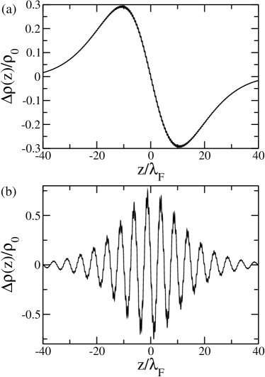
Figure 6: The charge density correction, $\Delta\rho(z)$, per electron per unit cell: $\rho_{0}=2e/\alpha$Cm^-1. The domain wall length is $\lambda=10\lambda_{F}$ with parameters for panels (a) and (b) as given in Fig. 4.

In case (a) we do see a charge build up, and respectively depletion, antisymmetric with respect to the center of the domain wall. The small “wiggles” on top of the overall charge rearrangement are caused by backward scattering. In case (b) we see strong oscillations of the charge density caused by forward scattering which are largest at the center of the domain wall. The very fast oscillations, which can be seen in more detail in Fig. 7, originate from back scattering.

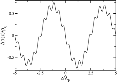
Figure 7: Same as Fig. 6(b) where we have zoomed in on a shorter length making the oscillations due to back-scattering clearly visible.

Finally, we note that the overall charge in the model is conserved, i.e., $\int\,\mathrm{d}z\Delta\rho(z)=0$. The total spin $\langle S^{2}\rangle$ in the system is also conserved and is related to the charge density: $\langle S^{2}(z)\rangle=\frac{3}{4e}\langle\rho(z)\rangle$. Therefore the total spin is redistributed throughout the wire in precisely the same way as the charge. However none of $S^{x}$, $S^{y}$, or $S^{z}$ are themselves conserved.

If we compare Fig. 6 to the results found by Dugaev et al., Ref. Dugaev et al., 2002, the most striking difference is the presence of strong Friedel oscillations. Such oscillations are well known and are already present in the non-interacting case. However, we also see that depending on parameters the amplitude of the Friedel oscillations can be quite small (see e.g. Fig. 6(a)) and might be easily overlooked if one mainly concentrates on the overall shape. Compared to the non-interacting caseTaniguchi et al. (2009) the spin density corrections have a different profile around the domain wall in the transverse direction. We want to stress that our model offers a method of calculating non-perturbatively the full effect of short range electron-electron interactions on any physical property we are interested in. Provided of course that one is in the regime of sufficiently high temperatures such that the perturbative analysis of the gauge potential remains valid. This includes, in particular, the physically important regime for quantum wires in ferromagnetic materials discussed above. In such systems, however, the phases of the extended domain wall regime (see table 1) should also be accessible.

We now want to briefly discuss consequences of the strong correlations in the electronic systems for the dynamics of the domain wall. The magnetization dynamics are described by the Landau-Lifschitz-Gilbert equation, or some suitable generalization thereof.Lifschitz and Pitaevskii (2002); Gilbert (2004); Zhang and Li (2004) There are two different aspects to this we must consider. One is the straightforward point that the dynamics, over the length of the wall, will be affected by the different spin density of the Luttinger liquid compared to the Fermi liquid or non-interacting case. The second, more interesting point, is whether the derivation of the non-adiabatic terms in the LLG equation are valid for a Luttinger liquid.

Following Zhang and LiZhang and Li (2004) one can derive contributions to the magnetization dynamics which allow for the fact that the electrons do not instantaneously follow the magnetization profile. One first writes a continuity equation for the spins, assuming part of it to be always parallel to the bulk magnetization and allowing a small deviation from this. In order to derive the current dependent (so called $\beta$-) terms, those which drive the domain wall along the wire, one assumes that $j^{x,y,z}_{s}(z,t)=-\mu_{B}Pj^{x,y,z}_{e}(z,t)n^{x,y,z}(z,t)/e$. $\vec{j}_{e}(z,t)$ is the charge current and $P$ is the magnitude of the polarization, whilst $\vec{j}_{s}(z,t)$ is the spin current. A quite reasonable assumption in a Fermi liquid, this of course starts to look more dubious in the case of a Luttinger liquid. In the standard Luttinger liquid model spin and charge are of course uncorrelated and possess different velocities. Thus this assumption would completely fail. For us the situation is not so simple as we do not have spin-charge separation, nonetheless what is obvious from our model is that spin and charge are not fully correlated. One is forced to work with the spin current and not the electric current and, as we have already seen, the spin degrees of freedom can behave rather differently for this model.

V Conclusion

We have investigated a Luttinger liquid coupled to a non-collinear ferromagnetic magnetization profile in the shape of a domain wall. The domain wall acts as a spatially extended magnetic impurity for the electrons and introduces both forward and backward scattering terms, active over the length of the domain wall. In contrast to the well studied case of point-like impurities in Luttinger liquids the finite extent of the domain wall introduces a whole new layer of complexity to the problem. In a renormalization group treatment of the scattering terms, one has to distinguish between an extended regime and a sharp regime at low temperatures where the domain wall effectively becomes a delta function. In the extended regime the scattering terms are bulk operators while they become boundary operators in the sharp regime. An operator relevant in the extended regime can therefore become irrelevant in the sharp regime.

Simplest to understand is the sharp regime. Here the spin-flip and potential forward scattering terms are irrelevant or marginal, respectively. The low-temperature fixed points are then determined by the spin-flip and potential back scattering terms which both can be either relevant or irrelevant. If both are irrelevant, then the fixed point is the Luttinger liquid if potential back scattering is only relevant for one spin channel with the other terms being irrelevant, then the fixed point is an effective spinless Luttinger liquid. In all other cases the fixed-point will be a spin and charge insulator. Depending on the relative relevance of the backscattering operators, the region of the insulator in the vicinity of the domain wall can show a reduced, increased or unaffected polarization in comparison to the bulk.

If we start with an extended domain wall, however, then the domain wall length $\lambda$ will usually be large compared to the backward scattering length $\lambda_{+}$, i.e., the backward scattering terms will strongly oscillate over the length of the domain wall. This means that the effective bare coupling—roughly proportional to the Fourier mode of the domain wall potential commensurate with the backward scattering oscillations—will be exponentially small $\sim\exp(-\lambda/\lambda_{+})$. So even if backward scattering is relevant, temperatures $T/J<\exp(-\lambda/\lambda_{+})$ are required in order to make this scattering process important. The sharp regime is therefore only physically relevant if we already start with a very sharp domain wall (of the order of a few lattice sites) which could possibly be realized by a nanoconstriction.

In the extended regime, the low temperature physics of the model is not only determined by the relevance or irrelevance of the various scattering terms but also by the hierarchy of the three different length scales present in the problem. Analyzing the first order RG equations for backward and forward scattering and taking the hierarchy of the three length scales into account we could identify three phases. If either, both the scattering terms are irrelevant, or they are relevant but the associated length scales are much smaller than the domain wall length $\lambda$, we find an adiabatic Luttinger liquid. In this case the spins of the electrons follow the magnetization profile and both charge and spin excitations are gapless. If both scattering terms are relevant and their respective length scales larger than $\lambda$ then the first order RG equations suggest that the system will become a spin-charge insulator, i.e., the domain wall will act as a perfectly reflecting barrier. This case corresponds to the normal Kane-Fisher fixed point. Finally, there is the case of forward scattering being relevant and the associated length scale being larger than $\lambda$, with backward scattering being either irrelevant or having an associated length scale which is smaller than $\lambda$. In this case the charge modes are gapless and charge is allowed to pass through the domain wall barrier. The spin modes, on the other hand, are locked to a specific value over the length of the domain wall and the system becomes insulating with respect to spin transport (C$1$S$0$ phase). Physically, this means that electrons no longer undergo a change of spin on passing through the domain wall. The latter phase has not been discussed so far in this context and it is this phase which we believe is most important in possible experimental realizations.

We also calculated the spin and charge densities around the domain wall for physically reasonable parameters in a regime at high enough temperatures so that even relevant scattering terms can be treated perturbatively. Here one finds spin and charge distributions markedly different to the previously reported mean field interaction case. Both the overall profile, and the local distribution, of spin and charge show different behaviour, including Friedel oscillations. A similar result to ours for the lateral component of spin is found in the non-interacting case,Taniguchi et al. (2009) though the transverse components look qualitatively different. As an outlook, we believe that it will be interesting to study how the dynamics of the domain wall is changed in this temperature range where correlation effects dramatically alter the spin and charge densities compared to the non-interacting case but where we are still far above the phase transition temperatures to the low-temperature phases discussed above.

Appendix A Details of the Rotations

The spin and charge Luttinger parameters are, to lowest orders:

$$v_{c} = \frac{v_{F\uparrow}+v_{F\downarrow}}{2}+\frac{g_{4\parallel\uparrow}+g_{4\parallel\downarrow}+2g_{4\perp}}{4\pi},$$

$$v_{s} = \frac{v_{F\uparrow}+v_{F\downarrow}}{2}+\frac{g_{4\parallel\uparrow}+g_{4\parallel\downarrow}-2g_{4\perp}}{4\pi},$$

$$K_{c} = 1-\frac{1}{2\pi}\frac{g_{2\parallel\uparrow}+g_{2\parallel\downarrow}+2g_{2\perp}}{v_{F\uparrow}+v_{F\downarrow}},$$

$$K_{s} = 1-\frac{1}{2\pi}\frac{g_{2\parallel\uparrow}+g_{2\parallel\downarrow}-2g_{2\perp}}{v_{F\uparrow}+v_{F\downarrow}},$$

$$v_{a} = \frac{v_{F\uparrow}-v_{F\downarrow}}{2}-\frac{g_{2\parallel\uparrow}-g_{2\parallel\downarrow}}{4\pi}+\frac{g_{4\parallel\uparrow}-g_{4\parallel\downarrow}}{4\pi}\textrm{, and}$$

$$v_{b} = \frac{v_{F\uparrow}-v_{F\downarrow}}{2}+\frac{g_{2\parallel\uparrow}-g_{2\parallel\downarrow}}{4\pi}+\frac{g_{4\parallel\uparrow}-g_{4\parallel\downarrow}}{4\pi}.$$ (30)

In order to enforce the condition $K_{s}=1$ at the $SU(2)$ symmetric point ($J=0$) we set

$$K_{s} = 1-\frac{1}{2\pi}\frac{g_{2\parallel\uparrow}+g_{2\parallel\downarrow}}{v_{F\uparrow}+v_{F\downarrow}},$$ (31)

canceling the $g_{2\perp}$ term by hand. It is clear that this $J$ independent term must cancel when higher order corrections are included. What we do not know in this low-order analysis is how the $J$ dependence of the Luttinger parameters will be modified by higher order terms.

The two rotations we use on the bosonic fields are

$$\begin{pmatrix}\phi_{\uparrow}\\ \phi_{\downarrow}\\ \theta_{\uparrow}\\ \theta_{\downarrow}\end{pmatrix}=\underbrace{\frac{1}{\sqrt{2}}\begin{pmatrix}-1&0&-1&0\\ 0&-1&0&-1\\ 1&0&-1&0\\ 0&1&0&-1\end{pmatrix}}_{=\mathcal{U}^{-1}}\begin{pmatrix}\phi_{\uparrow+}\\ \phi_{\downarrow+}\\ \phi_{\uparrow-}\\ \phi_{\downarrow-}\end{pmatrix}$$ (32)

and

$$\begin{pmatrix}\phi_{s}\\ \phi_{c}\\ \theta_{s}\\ \theta_{c}\end{pmatrix}=\underbrace{\frac{1}{\sqrt{2}}\begin{pmatrix}1&-1&0&0\\ 1&1&0&0\\ 0&0&1&-1\\ 0&0&1&1\end{pmatrix}}_{=\tilde{\mathcal{U}}^{-1}}\begin{pmatrix}\phi_{\uparrow}\\ \phi_{\downarrow}\\ \theta_{\uparrow}\\ \theta_{\downarrow}\end{pmatrix}.$$ (33)

To diagonalize the matrix $\tilde{M}$, Eq. (8), we perform two steps. The first is a rotation to make the Hamiltonian diagonal, characterized by the $R_{1,2}^{\theta,\phi}$ terms. The second is a rescaling to leave us with two distinct eigenvalues rather than four, this introduces the $\Gamma$’s. Together this gives us

$$\begin{pmatrix}\theta_{1}(z)\\ \theta_{2}(z)\end{pmatrix} = \begin{pmatrix}R^{\theta}_{1}\sqrt{\Gamma_{1}^{\theta}}&R^{\theta}_{2}\sqrt{\Gamma_{1}^{\theta}}\\ -R^{\theta}_{2}\sqrt{\Gamma_{2}^{\theta}}&R^{\theta}_{1}\sqrt{\Gamma_{2}^{\theta}}\end{pmatrix}\begin{pmatrix}\theta_{c}(z)\\ \theta_{s}(z)\end{pmatrix}\textrm{ and}$$

$$\begin{pmatrix}\phi_{1}(z)\\ \phi_{2}(z)\end{pmatrix} = \begin{pmatrix}R^{\phi}_{1}\sqrt{\Gamma_{1}^{\phi}}&R^{\phi}_{2}\sqrt{\Gamma_{1}^{\phi}}\\ -R^{\phi}_{2}\sqrt{\Gamma_{2}^{\phi}}&R^{\phi}_{1}\sqrt{\Gamma_{2}^{\phi}}\end{pmatrix}\begin{pmatrix}\phi_{c}(z)\\ \phi_{s}(z)\end{pmatrix}.$$ (34)

Here the rotation components are

$$2(R^{\theta}_{1,2})^{2} = 1\pm\bigg{[}1+\frac{v_{a}^{2}}{(\frac{v_{c}K_{c}}{2}-\frac{v_{s}K_{s}}{2})^{2}}\bigg{]}^{-\frac{1}{2}}\textrm{, and}$$

$$2(R^{\phi}_{1,2})^{2} = 1\pm\bigg{[}1+\frac{v_{b}^{2}}{(\frac{v_{c}}{2K_{c}}-\frac{v_{s}}{2K_{s}})^{2}}\bigg{]}^{-\frac{1}{2}}.$$ (35)

In order for the rotated Hamiltonian to have positive eigenvalues the condition $v_{c}v_{s}/v_{b}^{2}>K_{c}K_{s}>v_{a}^{2}/v_{c}v_{s}$ must also be satisfied. This condition seems to be always fulfilled, at least if one uses the integrable Hubbard model as the underlying microscopic lattice model.Penc and Sólyom (1993)

The rescaling of the fields requires

$$(\Gamma_{1,2}^{\phi})^{2} = (\Gamma_{1,2}^{\theta})^{-2}\textrm{, and}$$ (36)

$$(\Gamma_{1,2}^{\phi})^{2} = \frac{\frac{v_{c}}{2K_{c}}+\frac{v_{s}}{2K_{s}}\pm\sqrt{v_{b}^{2}+(\frac{v_{c}}{2K_{c}}-\frac{v_{s}}{2K_{s}})^{2}}}{\frac{v_{c}K_{c}}{2}+\frac{v_{s}K_{s}}{2}\pm\sqrt{v_{a}^{2}+(\frac{v_{c}K_{c}}{2}-\frac{v_{s}K_{s}}{2})^{2}}}.$$

Note that as the rotation is a unitary transformation we have the condition $[R^{\theta,\phi}_{1}]^{2}+[R^{\theta,\phi}_{2}]^{2}=1$. For our convenience we finally define

$$T^{\theta,\phi}_{1} = R^{\theta,\phi}_{2}/\sqrt{\Gamma_{1}^{\theta,\phi}},$$ (37)

$$T^{\theta,\phi}_{2} = R^{\theta,\phi}_{1}/\sqrt{\Gamma_{2}^{\theta,\phi}},$$

$$\tilde{T}^{\theta,\phi}_{1} = R^{\theta,\phi}_{1}/\sqrt{\Gamma_{1}^{\theta,\phi}}\textrm{, and}$$

$$\tilde{T}^{\theta,\phi}_{2} = -R^{\theta,\phi}_{2}/\sqrt{\Gamma_{2}^{\theta,\phi}}.$$

Therefore the inverse of Eq. (34) is

$$\begin{pmatrix}\phi_{c}(z)\\ \phi_{s}(z)\end{pmatrix} = \begin{pmatrix}\tilde{T}^{\phi}_{1}&\tilde{T}^{\phi}_{2}\\ T^{\phi}_{1}&T^{\phi}_{2}\end{pmatrix}\begin{pmatrix}\phi_{1}(z)\\ \phi_{2}(z)\end{pmatrix}\textrm{ and}$$

$$\begin{pmatrix}\theta_{c}(z)\\ \theta_{s}(z)\end{pmatrix} = \begin{pmatrix}\tilde{T}^{\theta}_{1}&\tilde{T}^{\theta}_{2}\\ T^{\theta}_{1}&T^{\theta}_{2}\end{pmatrix}\begin{pmatrix}\theta_{1}(z)\\ \theta_{2}(z)\end{pmatrix}.$$ (38)

Finally, the values of the new eigenvalues are

$$u_{1,2}^{2}=\bigg{(}\frac{v_{c}}{2K_{c}}+\frac{v_{s}}{2K_{s}}\pm\sqrt{v_{b}^{2}+\big{(}\frac{v_{c}}{2K_{c}}-\frac{v_{s}}{2K_{s}}\big{)}^{2}}\bigg{)}\qquad$$ (39)

$$\times\bigg{(}\frac{v_{c}K_{c}}{2}+\frac{v_{s}K_{s}}{2}\pm\sqrt{v_{a}^{2}+\big{(}\frac{v_{c}K_{c}}{2}-\frac{v_{s}K_{s}}{2}\big{)}^{2}}\bigg{)}.$$

As expected this reduces directly to the spin and charge excitation velocities in the absence of spin asymmetry. In such a case the Hamiltonian is already diagonal and the above rotation is no longer necessary.

The analytical result for the charge density correction is

$$\langle\Delta\rho(z)\rangle = \frac{e\operatorname{sech}[z/\lambda]}{2\pi mT\alpha\lambda}[T^{\phi}_{1}T^{\theta}_{1}+T^{\phi}_{2}T^{\theta}_{2}]\times$$

$$\bigg{[}g_{f}\sin[z/\lambda_{-}]\left(\frac{T}{T^{*}_{1}}\right)^{\alpha_{1}}\left(\frac{T}{T^{*}_{2}}\right)^{\alpha_{2}}$$

$$+g_{b}\sin[z/\lambda_{+}]\left(\frac{T}{T^{*}_{1}}\right)^{\beta_{1}}\left(\frac{T}{T^{*}_{2}}\right)^{\beta_{2}}\bigg{]}.$$

References

- Tomonaga (1950) S. Tomonaga, Progress of Theoretical Physics 5, 544 (1950).
- Luttinger (1963) J. M. Luttinger, Journal of Mathematical Physics 4, 1154 (1963).
- Giamarchi (2003) T. Giamarchi, Quantum Physics in One-Dimension (Oxford, 2003).
- Kane and Fisher (1992a) C. L. Kane and M. P. A. Fisher, Phys. Rev. Lett. 68, 1220 (1992a).
- Kane and Fisher (1992b) C. L. Kane and M. P. A. Fisher, Phys. Rev. B 46, 15233 (1992b).
- Eggert and Affleck (1992) S. Eggert and I. Affleck, Phys. Rev. B 46, 10866 (1992).
- Eggert and Affleck (1995) S. Eggert and I. Affleck, Phys. Rev. Lett. 75, 934 (1995).
- Rommer and Eggert (2000) S. Rommer and S. Eggert, Phys. Rev. B 62, 4370 (2000).
- Sirker et al. (2007) J. Sirker, N. Laflorencie, S. Fujimoto, S. Eggert, and I. Affleck, Phys. Rev. Lett. 98, 137205 (2007).
- Sirker et al. (2008) J. Sirker, S. Fujimoto, N. Laflorencie, S. Eggert, and I. Affleck, Journal of Statistical Mechanics: Theory and Experiment 2008, P02015 (2008).
- Penc and Sólyom (1993) K. Penc and J. Sólyom, Phys. Rev. B 47, 6273 (1993).
- Frahm and Korepin (1991) H. Frahm and V. E. Korepin, Phys. Rev. B 43, 5653 (1991).
- Marrows (2005) C. H. Marrows, Advances in Physics 54, 585 (2005).
- Parkin et al. (2008) S. S. P. Parkin, M. Hayashi, and L. Thomas, Science 320, 190 (2008).
- Dugaev et al. (2002) V. K. Dugaev, J. Barnaś, A. Łusakowski, and L. A. Turski, Phys. Rev. BSU 65, 224419 (2002).
- Araújo et al. (2006) M. A. N. Araújo, V. K. Dugaev, V. R. Vieira, J. Berakdar, and J. Barnaś, Phys. Rev. B 74, 224429 (2006).
- Araújo et al. (2007) M. A. N. Araújo, J. Berakdar, V. K. Dugaev, and V. R. Vieira, Phys. Rev. B 76, 205107 (2007).
- Pereira and Miranda (2004) R. G. Pereira and E. Miranda, Phys. Rev. B 69, 140402 (2004).
- Bruno (1999) P. Bruno, Phys. Rev. Lett. 83, 2425 (1999).
- Gambardella et al. (2002) P. Gambardella, A. Dallmeyer, K. Maiti, M. C. Malagoli, W. Eberhardt, K. Kern, and C. Carbone, Nature 416, 301 (2002).
- Shen et al. (1997) J. Shen, R. Skomski, M. Klaua, H. Jenniches, S. S. Manoharan, and J. Kirschner, Phys. Rev. B 56, 2340 (1997).
- Elmers et al. (1994) H. J. Elmers, J. Hauschild, H. Höche, U. Gradmann, H. Bethge, D. Heuer, and U. Köhler, Phys. Rev. Lett. 73, 898 (1994).
- Hauschild et al. (1998) J. Hauschild, H. J. Elmers, and U. Gradmann, Phys. Rev. B 57, R677 (1998).
- Wiesendanger (2009) R. Wiesendanger, Rev. Mod. Phys. 81, 1495 (2009).
- Mermin and Wagner (1966) N. D. Mermin and H. Wagner, Phys. Rev. Lett. 17, 1133 (1966).
- Jungwirth et al. (2006) T. Jungwirth, J. Sinova, J. Mašek, J. Kučera, and A. H. MacDonald, Rev. Mod. Phys. 78, 809 (2006).
- Natelson et al. (2000) D. Natelson, R. L. Willett, K. W. West, and L. N. Pfeiffer, Appl. Phys. Lett. 77, 1991 (2000). SU
- Granitzer et al. (2007) P. Granitzer, K. Rumpf, P. Pölt, A. Reichmann, M. Hofmayer, and H. Krenn, Journal of Magnetism and Magnetic Materials 316, 302 (2007), ISSN 0304-8853, proceedings of the Joint European Magnetic Symposia.
- Blundell (2009) S. Blundell, Magnetism in Condensed Matter (Oxford, 2009).
- Groot et al. (1983) R. Groot and F. Mueller, and P. Engen, and K. Buschow, Phys. Rev. Lett. 50, 2024 (1983).
- Tatara and Fukuyama (1997) G. Tatara and H. Fukuyama, Phys. Rev. Lett. 78, 3773 (1997).
- Korenman et al. (1977) V. Korenman, J. L. Murray, and R. E. Prange, Phys. Rev. B 16, 4032 (1977).
- Braunecker et al. (2009a) B. Braunecker, P. Simon, and D. Loss, Phys. Rev. Lett. 102, 116403 (2009a).
- Braunecker et al. (2009b) B. Braunecker, P. Simon, and D. Loss, Phys. Rev. B 80, 165119 (2009b).
- Negele and Orland (1998) J. W. Negele and H. Orland, Quantum Many-Particle Systems (Westview Press, 1998).
- Pereira (2004) R. G. Pereira, Master thesis, Universidade Estadual de Campinas Instituto de Fisica Gleb Wataghin (2004).
- Chudzinski et al. (2010) P. Chudzinski, M. Gabay, and T. Giamarchi, Phys. Rev. B 81, 165402 (2010).
- Fabrizio and Gogolin (1995) M. Fabrizio and A. O. Gogolin, Phys. Rev. B 51, 17827 (1995).
- Garate and Affleck (2010) I. Garate and I. Affleck, Phys. Rev. B 81, 144419 (2010).
- Balents and Fisher (1996) L. Balents and M. P. A. Fisher, Phys. Rev. B 53, 12133 (1996).
- Eggert and Rommer (1998) S. Eggert and S. Rommer, Phys. Rev. Lett. 81, 1690 (1998).
- Anfuso and Eggert (2006) F. Anfuso and S. Eggert, Phys. Rev. Lett. 96, 017204 (2006).
- Eggert et al. (2007) S. Eggert, O. F. Syljuasen, F. Anfuso, and M. Andres, Phys. Rev. Lett. 99, 097204 (2007).
- Sirker and Laflorencie (2009) J. Sirker and N. Laflorencie, Europhys. Lett. 86, 57004 (2009).
- Pereira et al. (2007) R. G. Pereira, J. Sirker, J.-S. Caux, R. Hagemans, J. M. Maillet, S. R. White, and I. Affleck, Journal of Statistical Mechanics: Theory and Experiment 2007, P08022 (2007).
- Taniguchi et al. (2009) T. Taniguchi, J. Sato, and H. Imamura, Phys. Rev. B 79, 212410 (2009).
- Lifschitz and Pitaevskii (2002) E. M. Lifschitz and L. P. Pitaevskii, Statistical Physics Part 2: Theory of the Condensed State (Butterworth-Heinemann, 2002).
- Gilbert (2004) T. Gilbert, IEEE Transactions on Magnetics 40, 3443 (2004).
- Zhang and Li (2004) S. Zhang and Z. Li, Phys. Rev. Lett. 93, 127204 (2004).