Two-photon decay of $\pi^{0}$ from two-flavor lattice QCD

Abstract:

We study the correction to the radiative $\pi^{0}$ decay width due to finite light quark mass. Using lattice QCD with the overlap fermion formulation, we calculate the three-point function of the form $\langle PV_{\mu}V_{\nu}\rangle$ in the (Euclidean) momentum space, which corresponds to the $\pi^{0}\rightarrow\gamma^{*}\gamma^{*}$ amplitude. To fit the lattice data, we use two different modifications of vector meson dominance (VMD) ansatz. One is a combined form of VMD with the next-to-leading order (NLO) chiral perturbation theory (ChPT), and the other is a resummed form of pion-loop diagrams. We extract one of the low energy constants in NLO ChPT, and estimate $\pi^{0}\rightarrow\gamma\gamma$ decay width.

1 Introduction

We present an update on our study [1] of the $\pi^{0}\rightarrow\gamma\gamma$ decay width using lattice QCD calculation of its off-shell amplitude. In the limit of massless up and down quarks, the corresponding amplitude is completely determined by the triangle anomaly [2, 3], which is valid to all orders in perturbation theory [4]. Once the quark mass is introduced, the correction term arises, which can be classified most conveniently in the effective field theory framework [5, 6]. The most recent analysis based on the next-to-next-to-leading order chiral perturbation theory including the isospin breaking effect [7] quoted $\Gamma_{\pi^{0}\gamma\gamma}$ = 8.09(11) eV, which marginally agrees with the recent experimental data $\Gamma_{\pi^{0}\rightarrow\gamma\gamma}$ = 7.82(22) eV [8]. The experimental error is expected to be reduced by a factor of 2 in the near future, and the improvement of the theoretical prediction would become more important. Presently, the theoretical estimate is limited by the lack of knowledge of the low energy constants in the effective theory, for which the lattice input is most desirable.

We calculate the $\pi^{0}\rightarrow\gamma^{*}\gamma^{*}$ (two photons are off-shell) amplitude in lattice QCD from the $\langle PV_{\mu}V_{\nu}\rangle$-type three-point function in the momentum space. In our previous report [1], we showed that the $\pi^{0}\rightarrow\gamma^{*}\gamma^{*}$ amplitude calculated on the lattice using the overlap fermion formulation is consistent with the expectation from the axial anomaly, which is $1/(4\pi^{2})$, after extrapolating to the limit of on-shell photons and massless quarks. The overlap fermion is most suitable for this study, because it has an exact U(1)_A chiral symmetry at the Lagrangian level that is violated by the quantum effect. Namely, it has the same symmetry structure as in the continuum theory even at finite lattice spacings.

We work on a two-flavor QCD ensemble of a $16^{3}\times 32$ lattice with the lattice cutoff $1/a$ = 1.667(17) GeV [10]. Dynamical quarks are also described by the overlap fermion. Topological charge $Q$ in this ensemble is fixed at $Q=0$, which is a source of the finite size effect [11]. There are four different quark masses, $m_{q}$ = 0.015, 0.025, 0.035, and 0.050 (in the lattice unit), which cover the range between $m_{s}/6$ and $m_{s}/2$ with physical strange quark mass $m_{s}$.

In the analysis presented last year [1], we used the naive vector meson dominance (VMD) ansatz to fit the lattice data and to extrapolate to the limit of on-shell photons. In the present report, we update this work including an analysis using other functional forms motivated by the chiral effective theories. We then present our preliminary result for the pion decay width.

Once the $\pi^{0}\rightarrow\gamma^{*}\gamma^{*}$ amplitude is determined including its off-shell form factor, it may be used to estimate the size of the light-by-light scattering contribution to the muon $g-2$, which occurs through a (probably dominant) virtual process $\gamma\gamma^{*}\to\pi^{0}\to\gamma^{*}\gamma^{*}$.

2 $\pi^{0}\rightarrow\gamma^{*}\gamma^{*}$ transition form factor

The $\pi^{0}\rightarrow\gamma^{*}\gamma^{*}$ transition form factor $f_{\pi^{0}\gamma^{*}\gamma^{*}}(p_{1},p_{2})$ is defined as a matrix element of two electromagnetic (vector) currents $V_{\mu}^{\rm EM}$ between the pion state and the vacuum:

$$\int\!d^{4}x_{1}d^{4}x_{2}e^{-ip_{1}x_{1}-ip_{2}x_{2}}\langle\pi^{0}(q)|V_{\nu}^{\rm EM}(p_{2})V_{\mu}^{\rm EM}(p_{1})|0\rangle=\varepsilon_{\mu\nu\alpha\beta}p_{1}^{\alpha}p_{2}^{\beta}f_{\pi^{0}\gamma^{*}\gamma^{*}}(p_{1},p_{2}),$$ (1)

where $p_{1}$ and $p_{2}$ denotes the off-shell photon momenta and $q=-p_{1}-p_{2}$. On the lattice we extract $f_{\pi^{0}\gamma^{*}\gamma^{*}}(p_{1},p_{2})$ from a three-point function

$$G^{PVV}_{\mu\nu}(P_{2},Q)=\sum_{x,y}e^{-iQx-iP_{2}y}\left\langle 2m_{q}P^{\rm rot\,3}(x)V^{\rm loc\,EM}_{\nu}(y)V^{\rm loc\,EM}_{\mu}(0)\right\rangle$$

$$=2m_{q}{\rm tr}[\tau^{3}Q_{e}^{2}]\left\langle\sum_{x,y,y^{\prime}}e^{-iQx-iP_{2}y}2{\rm Re}\,{\rm Tr}[S_{q}(0,x)\Gamma_{P}(x,y^{\prime})S_{q}(y^{\prime},y)\gamma_{\nu}S_{q}(y,0)\gamma_{\mu}]\right\rangle,$$ (2)

where $\langle\cdots\rangle$ denotes an ensemble average. $S_{q}(x,y)$ represents the quark propagator $D_{ov}(m)^{-1}(x,y)$ for the overlap-Dirac operator $D_{ov}(m)$ with the mass term $m$. To achieve the $O(a)$-improvement of the pseudoscalar density operator $P^{\rm rot\,3}$ contains the structure $\Gamma_{P}(x,y)=(1-D_{ov}(0)/M_{0})\gamma_{5}(x,y)$. “tr” means a trace over flavor indices, and “Tr” represents a trace over color and spinor indices. The (Euclidean) four-momenta $P_{1}$, $P_{2}$ and $Q(=-P_{1}-P_{2})$ are those of two photons and a pion, respectively. Their components are limited to discrete values $2\pi n_{\mu}/(L_{\mu}a)$, with the lattice spacing $a$ and the lattice size $L_{x,y,z}=16$ and $L_{t}=32$. In obtaining the second line of (2), we assumed that the disconnected quark diagrams are negligible.

With the overlap fermion formulation, the (flavor non-singlet) pseudo-scalar density operator $P^{\rm rot\,3}(x)=\bar{q}(x)\tau^{3}\gamma_{5}[(1-D_{ov}(0)/M_{0})q](x)$ satisfies the axial-Ward-Takahashi (AWT) identity $2m_{q}P^{\rm rot\,3}=\partial_{\mu}A_{\mu}^{\rm cv\,3}$ with the conserved axial-current $A_{\mu}^{\rm cv\,3}$ [12], which we numerically confirmed. For the electromagnetic current $V_{\mu}^{\rm loc\,EM}$ we use a local current defined with the overlap fermion field. The electromagnetic charge is assigned as $Q_{e}={\rm diag}\{2/3e,-1/3e\}$ for up and down quarks.

Because we use the sequential source method, we have to invert the overlap-Dirac operator for each choice of $P_{2}$, which is inserted at the point $y$. We restrict $P_{2}$ to the cases that it has a non-zero component only in the temporal direction, $P_{2}=(0,0,0,P_{2t})$, with $\nu=1$. Then we construct the three-point function by contracting the trace at the point $x$ with a momentum $Q=-P_{1}-P_{2}$ inserted. In order to minimize the numerical effort and the storage, we also restrict $P_{1}$ as

$$P_{1}=(0,P_{1y},0,0)\textrm{ when $\mu=3$} P_{1}=(0,0,P_{1z},0)\textrm{ when $\mu=2$},$$ or (3)

with all possible values of $P_{1y}$ and $P_{1z}$. With these choices, we can pick up the non-zero components of $P_{1\alpha}P_{2\beta}\varepsilon_{\mu\nu\alpha\beta}$ in (1).

We then extract the form factor $f_{\pi^{0}\gamma^{*}\gamma^{*}}(P_{1},P_{2})$ as

$$F^{\rm lat}(P_{1},P_{2}) = G^{PVV}_{\mu\nu}(P_{2},Q)\Big{/}\left(\sum_{\alpha\beta}P_{1\,\alpha}P_{2\,\beta}\varepsilon_{\mu\nu\alpha\beta}\right)=-\frac{f_{\pi}m_{\pi}^{2}}{Q^{2}+m_{\pi}^{2}}f_{\pi^{0}\gamma^{*}\gamma^{*}}(P_{1},P_{2})$$ (4)

up to the contributions from excited states and disconnected diagrams. Saturation of the pseudo-scalar channel by the pion field is quite accurate for small momenta, because the first excited state, called $\pi(1300)$ in PDG, is much heavier. We numerically confirmed this by looking at the two-point function $\langle PP\rangle$ in the momentum space.

Since $P_{1}$ and $P_{2}$ are defined in the Euclidean space-time, the on-shell condition is realized only at the zero momentum for both $P_{1}$ and $P_{2}$. In this limit, the three-point function trivially vanishes and no information on the form factor could be extracted. In order to obtain the decay width, we therefore have to work with slightly off-shell photons and to extrapolate to the on-shell limit assuming some functional form for $f_{\pi^{0}\gamma^{*}\gamma^{*}}(P_{1},P_{2})$.

3 Fit ansatz

For the form factor $f_{\pi^{0}\gamma^{*}\gamma^{*}}(P_{1},P_{2})$, a naive choice would be that of the vector dominance model (VMD)

$$F^{\rm VMD}(P_{1},P_{2})=-\frac{m_{\pi}^{2}}{Q^{2}+m_{\pi}^{2}}\frac{1}{4\pi^{2}}G_{V}(P_{1},m_{V})G_{V}(P_{2},m_{V}),$$ (5)

where $G_{V}(P,m_{V})=m_{V}^{2}/(P^{2}+m_{V}^{2})$ with the vector meson mass $m_{V}$. In the limit of $P_{1}=P_{2}=0$, (5) reduces to $1/4\pi^{2}$, which is the expectation of the anomaly valid in the massless limit. Note that the above approximation is too naive as the same value $1/(4\pi^{2})$ is also obtained even at finite quark mass, and so we clearly need modifications.

Apart from this limit, we expect some corrections. For small quark mass and external momenta, those can be described by the one-loop ChPT. A formula for the cases of off-shell photons is available in [13]. We slightly extend the formula by adding some analytic term and use a function

$$\Gamma^{\rm 1loop+VMD}(m_{\pi}^{2},P_{1}^{2}.P_{2}^{2}) = 1+\frac{1}{f_{\pi}^{2}}\Big{(}-\frac{4}{3}\Delta_{\pi}(m_{\pi}^{2})+J(m_{\pi}^{2},P_{1}^{2})+J(m_{\pi}^{2},P_{2}^{2})\Big{)}$$ (6)

$$-\frac{256\pi^{2}}{3}m_{\pi}^{2}y_{1}+\frac{64\pi^{2}}{3}\left(\frac{P_{1}^{2}}{P_{1}^{2}+m_{V}^{2}}+\frac{P_{2}^{2}}{P_{2}^{2}+m_{V}^{2}}\right)y_{2}$$

$$+\frac{P_{1}^{2}P_{2}^{2}}{(P_{1}^{2}+m_{V}^{2})(P_{2}^{2}+m_{V}^{2})}y_{3}$$

for $-4\pi^{2}F(P_{1},P_{2})/(m_{\pi}^{2}/(Q^{2}+m_{\pi}^{2}))$. (Namely, $\Gamma(m_{\pi}^{2},P_{1}^{2},P_{2}^{2})$ becomes 1 in the massless and soft photon limit.) Here, the first line in the above equation corresponds to the one-loop corrections. The tadpole diagram (Figure 1(a)) and the vector-vector correlator diagram (Figure 1(b)) lead to the following non-analytic functions

$$\Delta_{\pi}(m_{\pi}^{2}) = \frac{m_{\pi}^{2}}{16\pi^{2}}\ln\frac{m_{\pi}^{2}}{\mu^{2}},$$ (7)

$$J(m_{\pi}^{2},P^{2}) = \frac{2}{3}\left[\frac{P^{2}}{64\pi^{2}}\sigma^{2}\left\{-1+\ln\frac{m_{\pi}^{2}}{\mu^{2}}+2\sigma\tanh^{-1}\frac{1}{\sigma}\right\}-\frac{P^{2}+6m_{\pi}^{2}}{96\pi^{2}}\right],$$ (8)

respectively, with $\sigma=\sqrt{1+4m_{\pi}^{2}/P^{2}}$. The scale $\mu$ is the renormalization point that defines the counter terms. We set $\mu$ = 775 MeV, the physical $\rho$ meson mass.

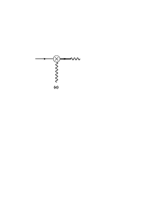
Figure 1: Vertices contribution to the $\pi^{0}\rightarrow\gamma^{*}\gamma^{*}$ decay. The solid, double-line and waved lines show pion, vector meson, and photon propagator, respectively.

The second and third lines of (6) define the analytic (or counter) terms. Since the lowest non-zero momentum $P_{1}^{2}\simeq$ 0.43 GeV² is already quite large to apply the one-loop ChPT formula, we modify the analytic terms motivated by VMD. Namely, the term with a single vector meson propagator (the forth term) represents the effective interaction of the form $\pi^{0}\gamma\rho$ (Figure 1(c)), while the last term represents $\pi^{0}\rho\omega$ (Figure 1(d)). The parameters $y_{1}$, $y_{2}$ and $y_{3}$ are to be determined by a numerical fit of the lattice data.

Another fit form we attempted is that of a resummed pion loops. Again motivated by VMD, we assume that the bubble diagrams shown in Figure 2 dominate the higher loop corrections and eventually produce the vector meson pole after summed up. Then, an expected functional form in the channel corresponding to the rho meson would be

$$\Gamma^{\rm resum}(m_{\pi}^{2},P_{1}^{2}.P_{2}^{2}) = 1-\frac{2}{f_{\pi}^{2}}\Delta_{\pi}(m_{\pi}^{2})-\frac{256\pi^{2}}{3}m_{\pi}^{2}z_{1}$$ (9)

$$+ \frac{L(m_{\pi}^{2},P_{1}^{2},z_{2})}{1-2L(m_{\pi}^{2},P_{1}^{2},z_{2})}+\frac{L(m_{\pi}^{2},P_{2}^{2},z_{2})}{1-2L(m_{\pi}^{2},P_{2}^{2},z_{2})},$$

$$L(m_{\pi}^{2},P^{2},z_{2}) = \frac{1}{f_{\pi}^{2}}\left(\frac{1}{3}\Delta_{\pi}(m_{\pi}^{2})+J(m_{\pi}^{2},P^{2})\right)+\frac{64\pi^{2}}{3}P^{2}z_{2},$$ (10)

where $z_{1}$ and $z_{2}$ are fit parameters.

Figure 2: Bubble diagram of pion loops. Symbols are the same as in Figure 1. Filled circle shows the tree-level vertex for the $\pi$-$\pi$ scattering diagram.

4 Fitting results

Here we describe the fit of the lattice data.

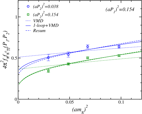
Figure 3: $\pi^{0}\rightarrow\gamma^{*}\gamma^{*}$ transition form factor as a function of pion mass squared. Different symbol denotes the different $(aP_{2})^{2}$, and $(aP_{1})^{2}$ is fixed in the lowest value, $0.154$. Thick solid and dashed curves are results in fit function $\Gamma^{\rm 1loop+VMD}$ and $\Gamma^{\rm resum}$ respectively. Thin dashed curve shows the naive VMD results as the comparison with them.

In order to keep the external momenta as small as possible, we restrict the momentum range to use, so that only $(aP_{1})^{2}=0.154$ and $0.039\leq(aP_{2})^{2}\leq 0.154$ are included. These correspond to the lowest $(aP_{1})^{2}$ and the lowest and second lowest $(aP_{2})^{2}$ in the momentum assignment (3). The data points are plotted in Figure 3 as a function of pion mass squared. The plot is normalized so that the on-shell limit corresponds to 1 in the chiral limit. So, we can see that the deviation from that limit is quite significant (as large as $\sim$ 50%).

By fitting the lattice data with the functions $\Gamma^{\rm 1loop+VMD}(m_{\pi}^{2},P_{1}^{2},P_{2}^{2})$ and $\Gamma^{\rm resum}(m_{\pi}^{2},P_{1}^{2},P_{2}^{2})$, we obtain the solid and dashed curves shown in Figure 3, respectively. Here we input the measured value of $m_{V}$ from two-point function $\langle VV\rangle$ into $\Gamma^{\rm 1loop+VMD}(m_{\pi}^{2},P_{1}^{2},P_{2}^{2})$. The naive VMD is also plotted by thin dashed curves for comparison. In the plot, one can see that both fit curves with the modified VMD show a better agreement with the lattice data than the naive VMD does, especially for the second lowest momentum.

	$y_{1}(=w_{3})$	$y_{2}$	$y_{3}$
1-loop + VMD	$-$0.00030(20) GeV-2	$-$0.0054(6)	1.65(48)
	$z_{1}(=w_{3})$	$z_{2}$
Resummation	$-$0.00120(12) GeV-2	$-$0.0271(37) GeV-2

Table 1: Fitting results with the function $\Gamma^{\rm 1loop+VMD}(m_{\pi}^{2},P_{1}^{2},P_{2}^{2})$ and with $\Gamma^{\rm resum}(m_{\pi}^{2},P_{1}^{2},P_{2}^{2})$. $y_{1}(z_{1})$ corresponds to LECs, $w_{3}$.

Fit parameters are listed in Table 1. A comparison with the phenomenological analysis in [13] is possible for the parameter controlling the pion mass dependence $w_{3}$, which corresponds to $y_{1}$ and $z_{1}$ in our functional form. Unfortunately, we find a significant discrepancy between $y_{1}$ and $z_{1}$. This suggests that the extraction of the low energy constants in the chiral effective theory from our calculation suffers from large systematic error. That is due to several possible reasons. One of them appears to be due to the large momentum we took for the off-shell photons to apply the one-loop ChPT. we estimate this parameter as $w_{3}=-0.00075(23)(63)\,{\rm GeV}^{-2}$, where the first error is statistical the second error denotes the systematic error coming from the ambiguity of the fit function. The phenomenological work used a value $w_{3}=0.0131$ [13], which is an order of magnitude larger than our result.

The $\pi^{0}\rightarrow\gamma\gamma$ decay width is defined as

$$\Gamma_{\pi^{0}\gamma\gamma}=\frac{m_{\pi}^{3}\alpha_{e}^{2}}{64\pi^{3}f_{\pi}^{2}}|\Gamma^{\rm fit}_{\textrm{on-shell}}|^{2}$$ (11)

with QED fine structure constant $\alpha_{e}=1/137$. Inserting the fitting results after taking $P_{1}^{2}=P_{2}^{2}=0$, which is consistent with CHPT formula in on-shell two photon decay, we obtain

$$\Gamma_{\pi^{0}\gamma\gamma}=7.98(6)(20)\,{\rm eV},$$ (12)

where the first error is statistical and the second is systematic one. While the systematic uncertainty is still rather large in our calculation, the result and its error are compatible with the present world average, 7.87(47) eV [9], and also with the recent experimental result 7.82(22) eV [8].

5 Conclusions

Lattice calculation of the $\pi^{0}\rightarrow\gamma^{*}\gamma^{*}$ decay amplitude is feasible for space-like momenta $p_{1}$, $p_{2}$ and $q$. We attempt a fit of the lattice data with the functional forms motivated by the NLO ChPT, from which we can in principle extract the low energy constants in the effective theory. With our current setup, however, the smallest non-zero momentum is already too large to safely apply the NLO ChPT, so that we have to introduce some model functions to extend the ChPT form to larger momenta. Our proposals partly motivated by the vector meson dominance ansatz describe the lattice data very well, but are not an unique choice. The result for the physical decay width thus has large systematic effect, but is already compatible with other estimates in the size of uncertainty. An extension to larger lattices and an introduction of the twisted boundary condition will improve this situation a lot, which is a subject of future studies.

Numerical calculations are performed on IBM System Blue Gene Solution and Hitachi SR11000 at High Energy Accelerator Research Organization (KEK) under a support of its Large Scale Simulation Program (No. 09/10-09). This work is supported by the Grant-in-Aid of the Japanese Ministry of Education (No. 20105002, 21105508, 21764002, 22011012, 22740183 ).

References

• [1] E. Shintani, S. Aoki, S. Hashimoto, T. Onogi and N. Yamada [JLQCD Collaboration], PoS LAT2009, 246 (2009) [arXiv:0912.0253 [hep-lat]].
• [2] S. L. Adler, Phys. Rev.  177, 2426 (1969).
• [3] J. S. Bell and R. Jackiw, Nuovo Cim.  A 60, 47 (1969).
• [4] S. L. Adler and W. A. Bardeen, Phys. Rev.  182, 1517 (1969).
• [5] J. Wess and B. Zumino, Phys. Lett.  B 37, 95 (1971).
• [6] E. Witten, Nucl. Phys.  B 223, 422 (1983).
• [7] K. Kampf and B. Moussallam, Phys. Rev.  D 79, 076005 (2009) [arXiv:0901.4688 [hep-ph]].
• [8] I. Larin et al. [PrimEx Collaboration], arXiv:1009.1681 [nucl-ex].
• [9] K. Nakamura et al. [Particle Data Group], J. Phys. G 37, 075021 (2010).
• [10] S. Aoki et al. [JLQCD Collaboration], Phys. Rev.  D 78, 014508 (2008) [arXiv:0803.3197 [hep-lat]].
• [11] S. Aoki, H. Fukaya, S. Hashimoto and T. Onogi, Phys. Rev.  D 76, 054508 (2007) [arXiv:0707.0396 [hep-lat]].
• [12] Y. Kikukawa and A. Yamada, Nucl. Phys.  B 547, 413 (1999) [arXiv:hep-lat/9808026].
• [13] B. Borasoy and R. Nissler, Eur. Phys. J.  A 19, 367 (2004) [arXiv:hep-ph/0309011].