Wavelet Ensemble Kalman Filters

Abstract

We present a new type of the EnKF for data assimilation in spatial models that uses diagonal approximation of the state covariance in the wavelet space to achieve adaptive localization. The efficiency of the new method is demonstrated on an example.

Wavelet Ensemble Kalman Filters

Data assimilation, EnKF, wavelet transform, Coiflet, diagonal approximation, orthogonal wavelets, FFT

1 Introduction

Incorporating new data into computations in progress is a well-known problem in many areas, including weather forecasting, signal processing, and computer vision. Sequential Bayesian techniques based on the state-space model are known as filtering or data assimilation [1, 2]. The probability distribution of the system state is advanced in time by the computational model, while data is incorporated from time to time by modifying the probability distribution of the state by an application the Bayes theorem. Gaussian probability distributions are represented by their mean and covariance. An assumed constant state covariance then yields the classical optimal statistical interpolation (OSI). The Kalman filter (KF) evolves the state covariance, but it needs to maintain the covariance matrix, so it is not suitable for high-dimensional systems. The ensemble Kalman filter (EnKF) [2] replaces the state covariance by sample covariance of an ensemble of simulations. The EnKF allows an implementation without any change to the model; the model only needs to be capable of exporting its state and restarting from the state modified by the EnKF. Convergence of the ensemble covariance to the state covariance is guaranteed in the large ensemble limit [3, 4], but a good approximation may require hundreds of ensemble members [2] because the covariance between physically distant variables is small, yet the sample covariance for a small ensemble has many large long-range terms. Localization techniques [5, 6, 7] improve the approximation by suppressing the long-range terms.

In [8, 9, 10], we have proposed an alternative approach, the fast Fourier transform (FFT) EnKF. The FFT EnKF assumes that the state is a random field that is approximately homogeneous in space. Then the covariance matrix in the frequency domain can be well represented by its diagonal, which gives a good approximation even for very small ensembles. However, the covariance is not represented well when it varies with location. The sample covariance can be used for the cross-covariance between different physical fields in the state [10], which, however, may again cause spurious long-range correlations.

In this paper we extend the spectral approach to the wavelet EnKF, resulting in an automatic localization that varies in space adaptively. We also introduce a new technique for automatic localization of the cross-covariances, based on a projection and a diagonalization in the spectral space. The efficiency of the new methods is demonstrated on an example.

2 Related work

Diagonal approximation of the covariance in the frequency space was proposed for weather fields [11]. Wavelets are well suited for approximation of meteorological fields [12], and the diagonal approximation was extended to wavelet spaces [13, 14, 15]. The Fourier domain KF [16] is the KF applied to independent frequency modes. The Laplace operator represented by a diagonal matrix in the frequency space was used for a fast OSI [10]. The inverse of the Laplace operator was proposed as a covariance model [17], but higher negative powers [10] yield better distributions.

3 The ensemble Kalman filter

The modeled quantity is the probability distribution of the state $u$, represented by an ensemble of simulation states $\left\{u_{1},\ldots,u_{N}\right\}$. A data vector $d$ is linked with the state $u$ by the observation matrix $H$ such that if the model and the data are correct, then $d=Hu$. The data error is assumed to have normal distribution with zero mean and known covariance $R$. When the data arrives, the ensemble is updated by

$$u_{k}^{a}=u_{k}+Q_{N}H^{\mathrm{T}}\left(HQ_{N}H^{\mathrm{T}}+R\right)^{-1}\left(d+e_{k}-Hu_{k}\right),$$ (1)

where $Q_{N}$ is the sample covariance computed from the ensemble, and the data perturbation vectors $e_{k}$ are sampled from the data error distribution. The ensemble members are then advanced in time by the model until the next data vector is to be assimilated. See [2] for details.

4 Orthogonal wavelet transform

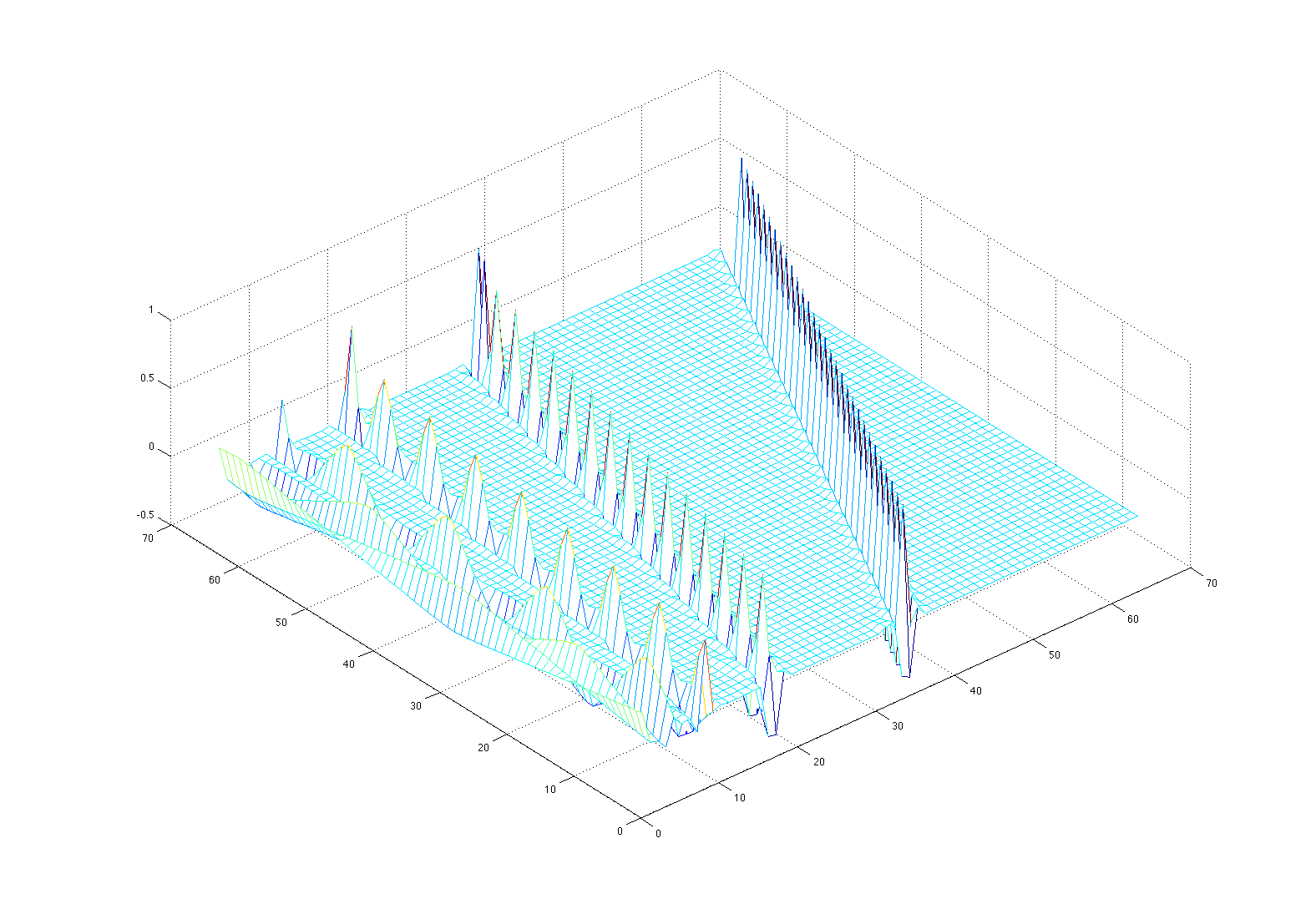
Figure 1: Wavelet transform matrix with $n=64$ and $5$ octaves, for the Coiflet 2 wavelet.

For vector $u$, denote $\widehat{u}=Fu$ the transform

$$\widehat{u}=\left[\widehat{u}_{\ell}\right]_{\ell=1}^{n},\quad\widehat{u}_{\ell}=f_{\ell}\cdot u,$$

where $f_{\ell}$ are the rows of $F$ and $F$ is orthonormal, $F^{-1}=F^{\mathrm{T}}$. Matrices are then transformed by

$$\widehat{M}=FMF^{-1}=FMF^{\mathrm{T}}.$$

In the FFT EnKF, we use the Fourier sine transform. In the wavelet EnKF, we use the orthogonal wavelet transform, where the rows of $F$ are $f_{\ell}=f_{\left(k,j\right)}$, given by values of the family of functions $\phi(2^{k}x-j)$ at the points $x=i/n$ for a total $n$ of composite indices $\ell=\left(k,j\right)$ such that $0\leq j\leq 2^{k}-1$. Each range of the indices $\left(k,j\right)$ with a fixed $k$ is called an octave. The function $\phi$ is called the mother wavelet and is chosen so that the rows $f_{\ell}$ are orthonormal. The indices need to span full octaves, which restricts the dimension $n$ to a power of $2$ (cf. Fig. 1), though generalizations are possible. See [18, 12] for further details. We use WaveLab [19] to perform the wavelet transform $\widehat{u}=Fu$ in Matlab. The complexity of the fast wavelet transform is only $O\left(n\right)$, compared to $O\left(n\log n\right)$ for the FFT.

In more than 1D, the spectral transformations are applied in each dimension separately, i.e., the basis functions are taken to be tensor products of 1D basis functions. Unlike in the case of the FFT, the tensor product of wavelets creates a certain bias for coordinate directions; the impact of this bias on specific applications must be examined [13]. However, 2D wavelets do not seem to be practical yet.

5 Spectral approximation of the covariance

5.1 Single variable

Consider first the case when the model state consists of one variable, in 1D only. Denote by $u\left(x_{i}\right)$, $i=1,\ldots,n$ the entry of the vector $u$, corresponding to node $x_{i}$. If the random field $u$ is stationary, then the covariance matrix satisfies $Q\left(x_{i},x_{j}\right)=c\left(x_{i}-x_{j}\right)$ for some covariance function $c$, and matrix-vector multiplication $v=Qu$ is the convolution,

$$v\left(x_{i}\right)=\sum_{j=1}^{n}Q\left(x_{i},x_{j}\right)u\left(x_{j}\right)=\sum_{j=1}^{n}u\left(x_{j}\right)c\left(x_{i}-x_{j}\right).$$

In the spectral domain, convolution becomes entry-by-entry multiplication of vectors, that is, the multiplication by a diagonal matrix, at least approximately.

Let $\widehat{u}_{ik}$ be the entries of the column vector $\widehat{u}_{k}=Fu_{k}$, i.e., ensemble member $k$ in the spectral space. Then we have the sample covariance in the spectral domain,

$$\widehat{C}(u,u) =FC(u,u)F^{-1}$$ (2)

$$=\frac{1}{N-1}{\sum_{k=1}^{N}F}\left(u_{k}-\overline{u}\right)\left(\widehat{u}_{k}-\overline{u}\right)^{\mathrm{T}}F^{-1}$$

$$=\frac{1}{N-1}{\sum_{k=1}^{N}}\left(\widehat{u}_{k}-\overline{\widehat{u}}\right)\left(\widehat{u}_{k}-\overline{\widehat{u}}\right),$$

where $\overline{\widehat{u}}=\frac{1}{N}\sum_{k=1}^{N}\widehat{u}_{k}$ is the sample mean. Assuming that the covariance is primarily a function of the physical distance between the nodes $x_{i}$, we approximate the forecast covariance in the spectral domain by the diagonal $\widehat{D}(u,u)$ of $\widehat{C}(u,u)$,

$$\left(\widehat{D}(u,u)\right)_{ii} =\frac{1}{N-1}{\sum_{k=1}^{N}}\left|\widehat{u}_{ik}-\overline{\widehat{u}}_{i}\right|^{2},$$ (3)

$$\left(\widehat{D}(u,u)\right)_{ij} =0\text{ for }i\neq j.$$

5.2 Multiple variables

When the model state consists of more than one variable, the covariance is split into blocks of cross-covariances between each variable. The diagonal blocks of the covariance can be approximated as in (3). Off-diagonal blocks cannot, in general, be treated the same way because the meshes over which different variables are defined may not coincide. In this case, we define an interpolation operator $P_{uv}$ that projects a variable $u$ to the mesh of variable $v$. While this matrix is rectangular in general, we require an approximate left inverse, such as the Moore-Penrose pseudoinverse, $P_{uv}^{\dagger}$, where $P_{uv}^{\dagger}P_{uv}\approx I$. In practice, more sophisticated and efficient methods with a sparse representation of the approximate left inverse are possible. In Section 7, we consider only cross-covariances between identical grids, leaving a more detailed examination of these techniques for future research.

By projecting $u$ to the grid of $v$, it is possible to proceed as in the single variable case and construct an approximate cross-covariance,

$$C(u,v)\approx P_{uv}^{\dagger}C(P_{uv}u,v)\approx P_{uv}^{\dagger}F^{-1}\widehat{C}\left(P_{uv}u,v\right)F.$$

6 Spectral EnKF

6.1 Single variable

First assume that the observation function $H=I$, that is, the whole state $u$ is observed. The evaluation of the EnKF formula (1) in the frequency domain, with the diagonal spectral approximation $\widehat{D}(u,u)$ of the covariance becomes

$$\widehat{u}^{a}=\widehat{u}+\widehat{D}(u,u)\left(\widehat{D}(u,u)+\widehat{R}\right)^{-1}\left(\widehat{d}+\widehat{e}-\widehat{u}\right).$$ (4)

The analysis ensemble is obtained by the inverse transform at the end, $u_{k}^{a}=F^{-1}\widehat{u}_{k}^{a}.$ Since $\widehat{D}$ is diagonal, (4) can be evaluated very efficiently in several important cases: (i) $\widehat{R}$ is diagonal; then $\widehat{D}+\widehat{R}$ is also diagonal and the evaluation of (4) reduces to term-by-term operations on vectors; (ii) $\widehat{R}$ is the perturbed data sample covariance and we can use the Sherman-Morrison-Woodbury formula, which only requires solving a system of dimension equal to the ensemble size $N$; (iii) $\widehat{R}$ is approximated by the diagonal part of the sample covariance in the spectral domain, just like the state covariance.

6.2 Multiple variables

Consider the state with multiple variables and the covariance and the observation matrix in the block form. Using the spectral covariance estimation in Sec. 5,

$$QH^{\mathrm{T}}=\left[C(u_{i},H_{j}u)\right]\approx P^{\dagger}F^{-1}\left[\widehat{D}(P_{i}u_{i},H_{j}u)\right]F,$$

with $P_{i}$ the interpolation operator from mesh $i$ to the observation grid, $P^{\dagger}$ the block diagonal matrix made up of $P_{1}^{\dagger},\cdots,P_{n_{v}}^{\dagger}$, and $F$ consisting likewise of the spectral transform in each variable. Similarly, we have $HQH^{\mathrm{T}}\approx F^{-1}\left[\widehat{D}(H_{i}u,H_{j}u)\right]F$, where the blocks are diagonal, so the term $HQH^{\mathrm{T}}+R$ in (1) can be inverted easily in the spectral domain. Since the cross covariances in the term $QH^{\mathrm{T}}$ in (1) are not involved in a matrix inversion, we can use another approximation, such the usual sample covariance [10], which may be more suitable when the field depends on the observed field non-locally, such as by advection.

7 Computational example

Variable $1$	Variable $2$
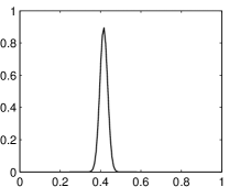
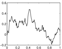
(a)	(b)

Figure 2: A single realization of the stochastic model.

We conclude with a simple example highlighting the advantages of the proposed method. We create a synthetic two-variable model state in one spatial dimension. Both variables are discretized on the same mesh of size $128$ over the domain $[0,1]$. The first variable is a simple Gaussian shape with random center, width, and height defined by

$$u_{1}(x)=h\exp(-\left(x-c\right)^{2}/w^{2}),$$ (5)

where $c\sim\mathcal{N}(0.3,0.1^{2})$, $w\sim\mathcal{N}(0.1,0.01^{2})$, and $h\sim\mathcal{N}(1,0.1^{2})$. The second variable is made up of the sum of two components. The first is a smooth random field made up of a sum of sine functions with random amplitudes. The amplitudes are sampled from a Gaussian distribution with variance decaying as the inverse square of the frequency. The second component is identical to the first variable scaled by $0.3$. The variables are chosen in this way so that the diagonal of $\operatorname*{Cov}(u_{1},u_{1})$ is non-uniform with a peak at $x=0.3$. Further, it is not obvious looking at a single realization (Figure 2) that the two variables are correlated; however, it is easily verified that $\operatorname*{Cov}(u_{1},u_{2})=0.3\operatorname*{Cov}(u_{1},u_{1})$.

Using a relatively small ensemble of size $10$, one can see from Figure 3 that both the FFT and wavelet covariance estimates decay to zero with distance as expected. In comparison to a large sample covariance (size $1000$), the spectral estimates offer a far better estimate of the true covariance than the traditional sample covariance when computed with the same ensemble. In addition, the wavelet covariance estimate correctly captures the spatial variability of the first variable’s distribution. This is in contrast to the FFT estimate that smooths the peak located at $0.3$ uniformly across the domain.

Large sample covariance	Small sample covariance
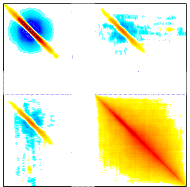
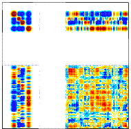
(a)	(b)
Covariance by FFT	Covariance by wavelets
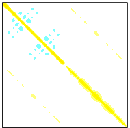
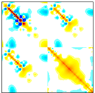
(c)	(d)

Figure 3: In (b)-(d), covariance estimates with an ensemble size $10$ are compared with the sample covariance of a large ensemble of size $1000$ in (a). The color scale is the same in each figure with positive and negative correlations displayed in red and blue, respectively.

In order to test the effectiveness of the spectral EnKF itself, we simulate an observation of the first variable with an observation grid that corresponds to the discretization of the model variables. We choose an observation generated from (5) with $c=0.4$, $w=0.12$, and $h=1.5$. We apply the spectral EnKF described in Section 6 with spectral transformations constructed from the discrete sine and Coiflet 2 wavelet transforms. We use same ensemble of size $10$ from Figure 3 for each assimilation test and choose a small data covariance $R=0.01^{2}I$ in order to force the assimilation to react visibly to the observation.

Figure 4 shows the forecast and analysis of the first ensemble member for each method. The data is displayed in each figure to help gauge the accuracy of the response of the observed peak at $x=0.4$. The traditional EnKF produces spurious noise near the peak of the forecast variable one, while the innovation in variable two is large throughout the domain rather than local to the observed peak. The FFT EnKF seems to react well to the observation in the second variable, but the first variable exhibits spurious noise similar to a Gibb’s effect throughout the domain. Finally, wavelet EnKF appears to provide the best analysis with very little spurious noise and a seemingly appropriate reaction to the observation.

EnKF	FFT EnKF	Wavelet EnKF
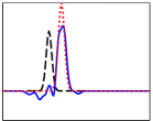
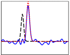
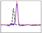
(a)	(b)	(c)
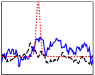
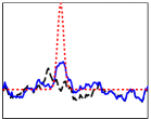
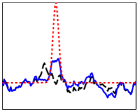
(d)	(e)	(f)

Figure 4: The first (a-c) and second (d-f) variables of a single ensemble member for each algorithm compared. The analysis is displayed as a solid blue line along with the forecast as a dashed black line and observation as a dotted red line.

8 Conclusion

Preliminary results indicate that the wavelet EnKF offers a vast improvement over the traditional assimilation techniques with similar ensemble sizes and without any localization needed. It requires only spatial information of the computational mesh, with no expert knowledge necessary to construct background covariances. Future work will analyze the effects of varying computational meshes as well as more complex observation functions on a range of operational computational models.

References

- [1] B. D. O. Anderson and J. B. Moore, Optimal filtering. Englewood Cliffs, N.J.: Prentice-Hall, 1979.
- [2] G. Evensen, Data Assimilation: The Ensemble Kalman Filter, 2nd ed. Springer Verlag, 2009.
- [3] J. Mandel, L. Cobb, and J. D. Beezley, “On the convergence of the ensemble Kalman filter,” arXiv:0901.2951, January 2009, To appear in Applications of Mathematics.
- [4] F. Le Gland, V. Monbet, and V.-D. Tran, “Large sample asymptotics for the ensemble Kalman filter,” INRIA Report 7014, August 2009.
- [5] R. Furrer and T. Bengtsson, “Estimation of high-dimensional prior and posterior covariance matrices in Kalman filter variants,” J. Multivariate Anal., vol. 98, no. 2, pp. 227–255, 2007.
- [6] B. Hunt, E. Kostelich, and I. Szunyogh, “Efficient data assimilation for spatiotemporal chaos: a local ensemble transform Kalman filter,” Physica D: Nonlinear Phenomena, vol. 230, pp. 112–126, 2007.
- [7] J. L. Anderson, “An ensemble adjustment Kalman filter for data assimilation,” Monthly Weather Review, vol. 129, pp. 2884–2903, 2001.
- [8] J. Mandel, J. Beezley, L. Cobb, and A. Krishnamurthy, “Data driven computing by the morphing fast Fourier transform ensemble Kalman filter in epidemic spread simulations,” Procedia Computer Science, vol. 1, no. 1, pp. 1215–1223, 2010.
- [9] J. Mandel, J. D. Beezley, and V. Y. Kondratenko, “Fast Fourier transform ensemble Kalman filter with application to a coupled atmosphere-wildland fire model,” in Computational Intelligence in Business and Economics, Proceedings of MS’10, A. M. Gil-Lafuente and J. M. Merigo, Eds. World Scientific, 2010, pp. 777–784.
- [10] J. Mandel, J. D. Beezley, K. Eben, P. Juruš, V. Y. Kondratenko, and J. Resler, “Data assimilation by morphing fast Fourier transform ensemble Kalman filter for precipitation forecasts using radar images,” CCM Report 289, University of Colorado Denver, April 2010, http://ccm.ucdenver.edu/reports/rep289.pdf.
- [11] L. Berre, “Estimation of synoptic and mesoscale forecast error covariances in a limited-area model,” Monthly Weather Review, vol. 128, no. 3, pp. 644–667, 2000.
- [12] A. Fournier, “Introduction to orthonormal wavelet analysis with shift invariance: Application to observed atmospheric blocking spatial structure,” Journal of the Atmospheric Sciences, vol. 57, no. 23, pp. 3856–3880, 2000.
- [13] A. Deckmyn and L. Berre, “A wavelet approach to representing background error covariances in a limited-area model,” Monthly Weather Review, vol. 133, no. 5, pp. 1279–1294, 2005.
- [14] A. Fournier and T. Auligné, “Development of wavelet methodology for WRF data assimilation,” Presentation given at University of Colorado Denver, November 2010, http://ccm.ucdenver.edu/wiki/File:Fournier-nov15-2010.pdf.
- [15] O. Pannekoucke, L. Berre, and G. Desroziers, “Filtering properties of wavelets for local background-error correlations,” Quarterly Journal of the Royal Meteorological Society, vol. 133, no. 623, Part B, pp. 363–379, 2007.
- [16] E. Castronovo, J. Harlim, and A. J. Majda, “Mathematical test criteria for filtering complex systems: plentiful observations,” J. Comput. Phys., vol. 227, no. 7, pp. 3678–3714, 2008.
- [17] P. K. Kitanidis, “Generalized covariance functions associated with the Laplace equation and their use in interpolation and inverse problems,” Water Resour. Res., vol. 35, no. 5, pp. 1361–1367, 1999.
- [18] M. V. Wickerhauser, Adapted wavelet analysis from theory to software. Natick, MA, USA: A. K. Peters, Ltd., 1994.
- [19] J. B. Buckheit and D. L. Donoho, “WaveLab and reproducible research,” Department of Statistics, Stanford University, 1995.