Realtime calibration of the A4 electromagnetic lead fluoride (PbF₂) calorimeter

Abstract

Sufficient energy resolution is the key issue for the calorimetry in particle and nuclear physics. The calorimeter of the A4 parity violation experiment at MAMI is a segmented calorimeter where the energy of an event is determined by summing the signals of neighbouring channels. In this case the precise matching of the individual modules is crucial to obtain a good energy resolution. We have developped a calibration procedure for our total absorbing electromagnetic calorimeter which consists of 1022 lead fluoride (PbF₂) crystals. This procedure reconstructs the the single-module contributions to the events by solving a linear system of equations, involving the inversion of a 1022$\times$1022-matrix. The system has shown its functionality at beam energies between 300 and 1500 MeV and represents a new and fast method to keep the calorimeter permanently in a well-calibrated state.

1 Introduction

The calibration procedure described here has been developed for the total absorbing homogenous electromagnetic calorimeter of the A4 experiment at the Mainz electron accelerator facility MAMI. The A4 collaboration investigates single spin asymmetries in the cross section of the elastic scattering of polarized electrons off unpolarized hydrogen and deuterium [1, 2, 3, 4]. In order to separate elastic scattering events from inelastic background, the energy of the detected particles is measured by means of a totally absorbing electromagnetic calorimeter. For such a a measurement, the analog signals of nine neighbouring modules are summed to form the event signal which is then digitized. It is obvious that a coherent signal response of all calorimeter modules is decisive to obtain an optimal energy resolution.

For the calibration of an electromagnetic calorimeter various methods are applicable. One common method is to use a radioactive source which delivers well-known energies up to a few MeV [5]. For a total absorbing calorimeter which measures energies in the range between several hundred MeV and a few GeV, however, no suitable radioactive sources exist. Another possible procedure uses direct photoelectrons. Light produced by UV lasers or LEDs is guided to the calorimeter modules by fibers [7]. However, the precision of this method is limited by the uniformity of the coupling of the fibers to the calorimeter crystals, the homogenity of the light sources and the losses in the individual fibers that determines the light input variation from crystal to crystal. A third common technique is the use of cosmic events for calibration purposes [6].

The method presented here is based on a calibration using elastically scattered electrons which are easy to identify and have well-defined energies. A difficulty arises from the fact that the data used to determine the current calibration state are not individual signals of single modules. Only the sum of the signals of nine neighbouring modules is accessible. The reconstruction of the individual yields of the modules involves linear algebra and is one of the main tasks in the calibration procedure.

2 The electromagnetic homogenous lead fluoride calorimeter

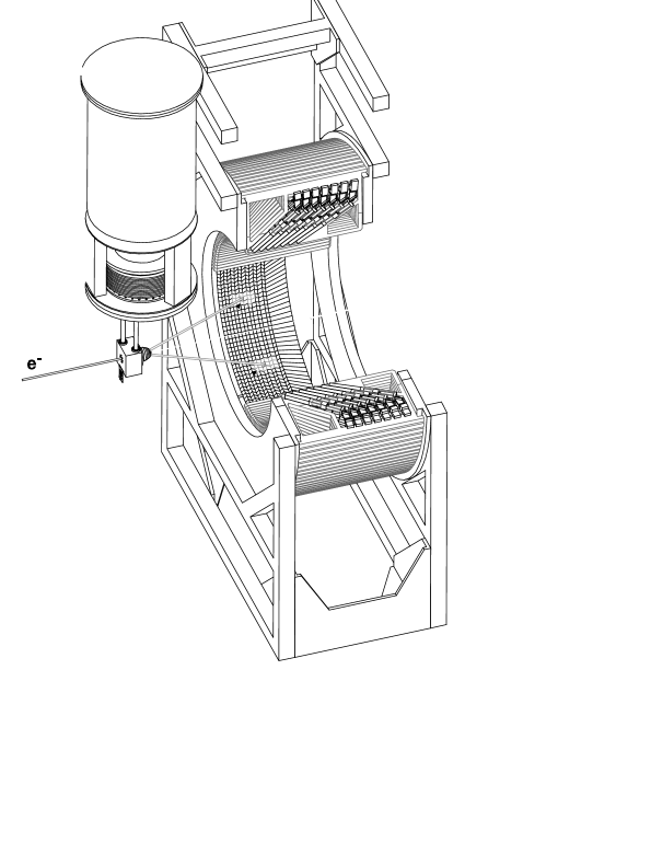
Figure 1: Partly cut-away view of the lead fluoride calorimeter. The electrons come from the left, hit the hydrogen target and are scattered into the calorimeter at polar angles of $30^{\circ}\leq\theta_{e}\leq 40^{\circ}$. The resulting electromagnetic shower is contained within a cluster of 3$\times$3 PbF₂ crystals.

The calorimeter consists of 1022 individual lead fluoride (PbF₂) crystals mounted on 146 aluminium frames and arranged in 7 rings (fig. 1). PbF₂ is a pure Cherenkov radiator with high transmission down to 270 nm [8]. Its radiation length is $X_{0}=0.93$ cm and its effective “Molière radius” for the production of Cherenkov photons from an electromagnetic shower is $R_{M}=1.8$ cm. The light is read out by photomultiplier tubes XP 2900 with borosilicate windows and transistorized, actively stabilized bases. We employ seven types of trapezoid-shaped PbF₂ crystals with slightly different shapes. The calorimeter geometry is that of a barrel with the individual crystals pointing to the target. The crystals have a cross section of 2.6 cm x 2.6 cm at the front, 3.0 cm x 3.0 cm at the back, and a length of 15–18 cm. In longitudinal direction we have chosen the crystal length to cover more than 15 radiation lengths in order to minimize shower leakages. In the transverse direction we have chosen a crystal width of 4/3 $R_{M}$. Hence, more than 95% of the Cherenkov light of an event is emitted in a cluster of 3$\times$3 crystals. The signals of all channels within this cluster are summed up for the energy measurement of an event (fig. 2). If another particle hits the same crystal (dark gray) during the integration window of 20 ns, a veto logic detects this double hit as long as the time lag between the two events is at least 6 ns. Also, during the integration time no other particle may hit the area around this cluster (light gray), because the electromagnetic shower of this event would overlap with that from the first particle. Both types of pile-up events would lead to a wrong energy determination and are rejected.

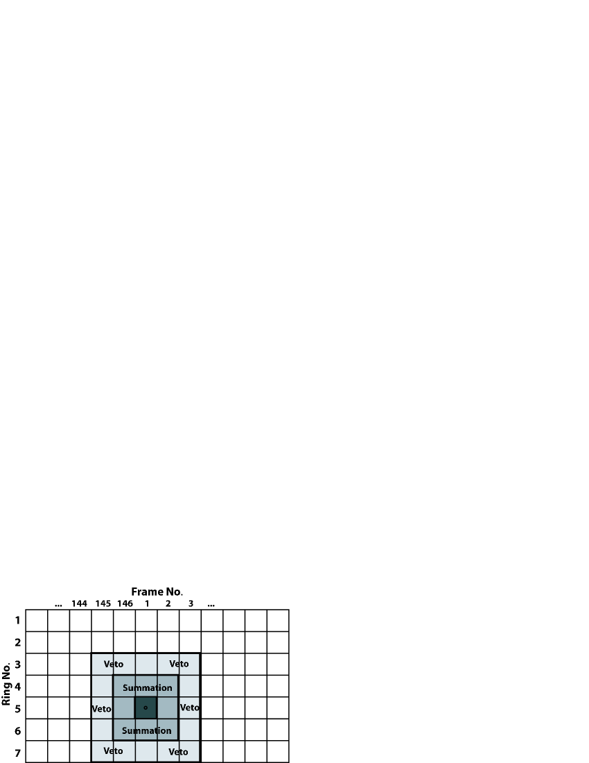
Figure 2: Schematic view of the array of lead fluoride crystals in the calorimeter. The modules are labelled according to the aluminium frame they are mounted on (1 to 146) and the ring they belong to (1 to 7). In this example, a particle hits the calorimeter at frame 1, ring 5 (marked in dark gray). In order to determine the energy of this event, the signal of this module and the signals of the eight neighbouring modules are summed up (medium gray). During the integration time no other particle may hit the area around this cluster (light gray), because the electromagnetic shower of this event would overlap with that from the first particle. In the case of such a pile-up both events are rejected.

Triggering, pile-up rejection, summing up the signals and storing them at event rates of up to 100 MHz requires parallelized electronics [9]. For each of the 1022 channels of the calorimeter there is a dedicated electronic circuit (fig. 3) implementing the event detection as follows: when a particle hits the calorimeter and deposits energy in the crystals around the impact zone, the trigger electronics of each of those modules recognizes the hit in the calorimeter. The center of the impact is determined by finding the crystal with the largest signal pulse height (Local Maximum, LM). This crystal defines the center of a 3$\times$3 cluster of crystals. The signals of the photomultiplier tubes of these nine crystals are summed up by an analog summation circuit. If this sum exceeds the trigger level of a constant fraction discriminator (Constant Fraction, CFD) and there is neither a double hit in the central crystal recognized by the pulse shaper unit (Pulse Shaper, PS) nor a second hit in the neighbouring modules, then a trigger flag is set. The signal of the 3$\times$3-cluster is digitized by an 8-bit ADC, the signal of the central crystal is additionally digitized by a 6-bit ADC and both values are stored in a histogramming unit. After a specified run time — usually 5 minutes — the histogram is read out and transferred to a storage device.

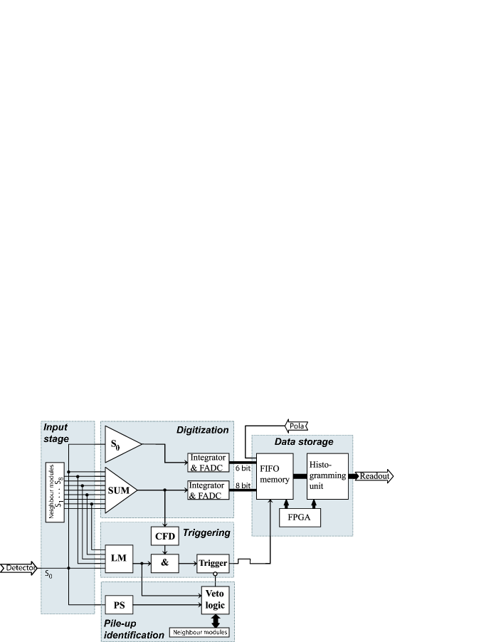
Figure 3: Diagram of the readout electronics [10]. The input signal from the photomultiplier tube is denoted with $S_{0}$. The signals of the neighbouring channels are denoted with $S_{1}$ to $S_{8}$. The signals are summed up by a summation amplifier. A triggering and a veto unit decide whether the event is stored into the histograms.

3 The calibration procedure

The aim of the calibration is to normalize the gain for all 1022 modules of the calorimeter: the same amount of energy deposited in a PbF₂ crystal should result in the same integrated current, i.e. collected charge, in the photomultiplier tubes (PMT) for all modules. Prior to installing the PMTs into the calorimeter, all of them were precalibrated in a test stand. The transit times were measured and the signal cable lengths adjusted to ensure an equal timing. Also, precision electronic parts were used in the summation circuits, e.g. resistors with 0.1% tolerance and capacitors with 1% tolerance. Even with low tolerance parts fitted into the calorimeter, the individual gains may still differ because of different light yields of the individual lead fluoride crystals or because of differences in the optical couplings between crystal and PMT. These residual differences are eliminated by adjusting the gains of the individual modules by varying the high voltage of the PMT. In order to determine these gains, we use the energy spectra which are measured during regular data taking. During data taking, there are two types of histograms available: The histograms from the 6-bit ADC which give the energy information of the single modules and the histograms from the 8-bit ADC which contain the summed energy information of a 3$\times$3-cluster of crystals. The histograms shown in fig. 4 are examples of such spectra. At large ADC values one can see the peak of elastic scattering events.

Figure 4: Typical energy spectra of the PbF₂ calorimeter: (a) Histogram of the 6-bit ADC with the signal of a single module, (b) Histogram of the 8-bit ADC with the signals of the modules of a 3$\times$3-cluster summed up. One can identify the peak of the elastically scattered electrons which corresponds to an energy of 734 MeV at around ADC channel 48 in (a) and around ADC channel 170 in (b). The cutoff at low ADC values is a threshold effect in the electronics. Due to the limited resolution of the 6-bit histogram we use the 8-bit histograms for the analysis where the signals of a 3$\times$3-cluster were summed up.

The cutoff at low ADC values is a threshold effect in the electronics. The offsets are measured in a separate procedure [10] and are located around ADC channel 32 for the 6-bit histogram and between ADC channels -25 and +10 for the 8-bit histograms. Due to the limited resolution of the 6-bit histogram we use the 8-bit histograms for the analysis. Since the energy of the electrons after elastic scattering is fixed by the kinematics, the position of the elastic peak given in ADC units together with the measured offset allows an unambiguous determination of the gain of a 3$\times$3-cluster in units of ADC/MeV. In order to disentangle the contributions of the single modules to this sum signal, one needs to understand how the energy of an event is deposited within the cluster. With the knowledge of the average lateral distribution of the electromagnetic shower, one can set up a system of equations which relates the sum signals to the individual gains of the single modules. By solving this system of equations, one can determine the individual amplification factors. The latter can be used to calculate a new set of high voltages for the photomultipliers necessary to reach the desired calibration state.

The following steps are necessary for the calibration procedure. They will be discussed in detail in the remainder of this chapter:

1. Understand and parameterize the lateral distribution of the electromagnetic shower in the PbF₂ calorimeter.

2. Analyze the 1022 energy spectra to find the position of the elastic peak which gives the information about the signal gain for a whole 3$\times$3 cluster

3. Using the methods of linear algebra, solve the equations and calculate the amplification factors of the individual single modules

4. Calculate and apply new high voltages to reach the desired amplification for all modules

3.1 Lateral distribution of the electromagnetic shower in the calorimeter

When a scattered electron with an energy of several hundred MeV hits a calorimeter module, it will lose its kinetic energy developing an electromagnetic shower where bremsstrahlung and pair production are the dominant processes. Since the crystals have a length of at least 15 radiation lengths, electrons with energies up to 1 GeV will be absorped completely in the calorimeter and there is no concern about the longitudinal distribution of the shower. The transverse development of the electromagnetic shower scales with the Molière radius $R_{M}$. About 90% of the energy is deposited within a cylinder with radius $R_{M}$. The lateral energy distribution of the electromagnetic shower can be parameterized using a sum of two exponentials [11]:

$$f(r)=a_{1}\exp\left(-r/b_{1}\right)+a_{2}\exp\left(-r/b_{2}\right)$$ (1)

For our calorimeter material, lead fluoride, these coefficients have been determined by GEANT simulations [12]. Normalizing $f(r)$ to one,

$$\int\limits_{0}^{2\pi}\int\limits_{0}^{\infty}rf(r)\,d\phi\,dr=1$$ (2)

one gets $a_{1}=2.41~{}\mathrm{mm}^{-2}$, $a_{2}=0.19~{}\mathrm{mm}^{-2}$, $b_{1}=1.5~{}\mathrm{mm}$ and $b_{2}=7.4~{}\mathrm{mm}$ (fig. 5).

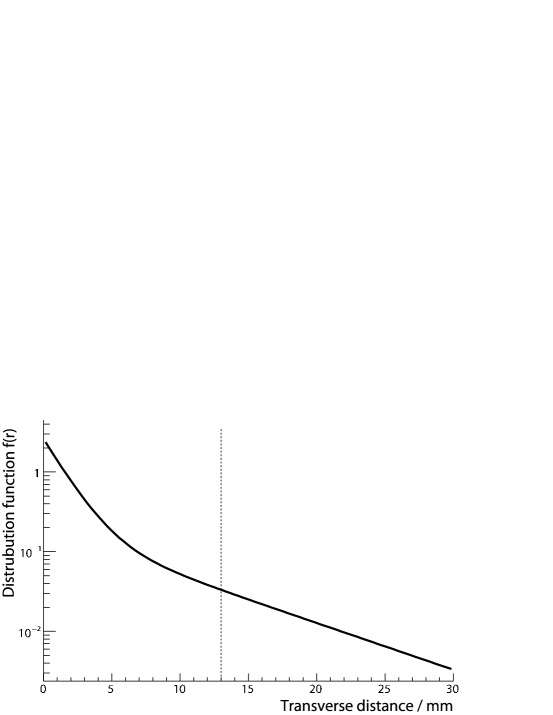
Figure 5: Lateral distribution (eq. 1) of the energy of an electromagnetic shower in lead fluoride, where the parameters $a_{1}$, $a_{2}$, $b_{1}$ and $b_{2}$ were determined by a GEANT simulation. The dotted line indicates the limit of the crystal surface whereas the origin of the x-axis lies on the center of the crystal.

With this shower distribution function one can calculate the amount of energy that is deposited on average in the modules of a 3$\times$3 cluster whose central crystal has been hit by a scattered particle. There are three “types” of crystals in such a cluster (fig. 6):

Figure 6: Schematic representation of a 3$\times$3 cluster of crystals. There are three “types” of modules, the central crystal (no. 0) which defines the 3$\times$3 cluster, the direct neighbours (no. 1,3,5,7) and the diagonal neighbours (no. 2,4,6,8). The fraction of energy that is deposited on average in these three classes of crystals is denoted by $\mu_{c}$, $\mu_{n}$ and $\mu_{d}$ respectively.

the central crystal c (no. 0) which defines the 3$\times$3 cluster, the direct neighbours n (no. 1,3,5,7) and the diagonal neighbours d (no. 2,4,6,8). How the energy is spread out over the modules for a single event depends on the impact position of the incident particle as well as on the actual development of the electromagnetic shower which is subject to statistical fluctuations. However, since the calibration is performed using a histogram of a large number of events (between $10^{6}$ and $10^{7}$ events), only the average of that distribution over all possible impact positions and over a large number of electromagnetic showers is relevant. The fraction of energy that is deposited on average in these three classes of crystals is denoted by the distribution parameters $\mu_{c}$, $\mu_{n}$ and $\mu_{d}$, respectively:

$$E_{\rm{deposit}}=\left(\mu_{c}+4\mu_{n}+4\mu_{d}\right)E_{\rm{incident}}$$ (3)

These parameters can be determined by averaging the energy deposition of the electromagnetic shower over all possible impact positions on the central crystal’s surface. We assume that within one crystal all impact positions have equal probability which is a good approximation considering the small single-crystal acceptance:

$$\mu_{c,n,d}=\frac{1}{S_{c}}\,\int\limits_{S_{c}}\;\>\int\limits_{S_{c,n,d}}f(x^{\prime}-x,y^{\prime}-y)\,dx^{\prime}\,dy^{\prime}\,dx\,dy$$ (4)

The $S_{c,n,d}$ denote the surface of the center, neighbour or diagonal crystal, respectively, $f(x,y)=f(r)$ with $r=\sqrt{x^{2}+y^{2}}$ parameterizes the lateral energy deposition of the electromagnetic shower (eq. 1). We have computed this integral using the actual dimensions of the crystals. The parameters are $\mu_{c}=65.3\%$, $\mu_{n}=6.2\%$ and $\mu_{d}=1.2$%. On average, the biggest fraction of energy is deposited in the central crystal, while the diagonal neighbours contribute only 1.2% each.

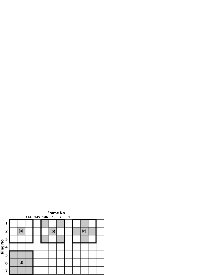
Figure 7: Method for a measurement of the distribution parameters $\mu$ with the electron beam. The colored boxes indicate modules which are supplied with high voltages: (a) Only the central crystal, (b) the central crystal and its diagonal neighbours, (c) the central crystal and its direct neighbours, (d) all modules of a 3$\times$3 cluster.

We also performed a measurement of the distribution parameters $\mu_{c,n,d}$. The method is to supply only the PMTs of selected modules of a 3$\times$3-cluster with high voltages (fig. 7). In this way the other modules, either the direct neighbours or the diagonal neighbours or all neighbours, do not contribute to the signal, resulting in a shift of the position of the elastic peak in the ADC spectra (fig. 8). Measuring this shift, the contribution of neighbouring modules can be determined.

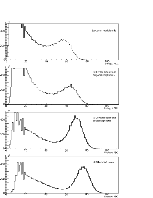
Figure 8: PbF₂ spectra used for measuring the distribution parameters $\mu$. The beam energy was 510 MeV. The spectra were obtained applying the HV supply patterns of fig. 7. When the contribution of neighbouring modules are included, the shift of the elastic peak to higher ADC values is clearly visible.

Several of these spectra were analyzed. The offset-corrected position of the elastic peak (see sec. 3.2 on how the positions were determined) is denoted by $P_{3\times 3}$ when all modules were on (fig. 7d), $P_{cn}$ when the central module and its direct neighbours were on (fig. 7c), $P_{cd}$ when central module and its diagonal neighbours were on (fig. 7b )and $P_{c}$ when only the central module was on (fig. 7a). Then one can calculate the distribution parameters as follows:

$$\mu_{c}=0.95\cdot\frac{P_{c}}{P_{3\times 3}},\,\,\,\mu_{n}=0.95\cdot\frac{1}{4}\frac{P_{cn}-P_{c}}{P_{3\times 3}},\,\,\,\mu_{d}=0.95\cdot\frac{1}{4}\frac{P_{cd}-P_{c}}{P_{3\times 3}}$$ (5)

The factor of 0.95 is used to take into account the lateral energy leakage which is included in the calculation based on eq. 1 but which cannot be measured by the method described here. The results are summarized in table 1. The quoted uncertainties are statistical only.

Parameter	Measurement	Calculation
$\mu_{c}$	(64.1 $\pm$ 0.3${}_{\rm{\,stat}}$) %	65.3 %
$\mu_{n}$	( 5.3 $\pm$ 0.1${}_{\rm{\,stat}}$) %	6.2 %
$\mu_{d}$	( 2.3 $\pm$ 0.1${}_{\rm{\,stat}}$) %	1.2 %

Table 1: Results of the measurement of the distribution parameters. The quoted uncertainties are statistical only. The calculation following eq. 4 is based on the parameterization of the lateral shower distribution according to eq. 1.

The values from the measurement differ slightly but significantly from those resulting from the calculation based on the lateral shower distribution. On the one hand, the parameterization of the shower distribution eq. 1 might not describe perfectly the actual averaged shower distribution in lead fluoride. On the other hand, systematic errors of the measurement are not included here: the trigger conditions change when some modules are not supplied with high voltages. Furthermore, the local maximum (LM) and the absence of a pile-up veto is necessary for accepting an event. These conditions are different for each of the high voltage patterns, which adds an additional systematic uncertainty to the measurement of the distribution parameter $\mu_{c}$, $\mu_{n}$ and $\mu_{d}$. Altogether, the agreement is good enough since the differences are small enough to be irrelevant for the calibration procedure.

3.2 Analyzing the energy spectra

In order to extract the information about the actual gains of calorimeter modules, the energy spectra have to be analyzed. Although fitting is a common method to do so, we do not use it for two reasons: first, due to the large number of spectra per run a complete fitting to all spectra is too time consuming for an online calibration with 10 seconds only of available time, and second, a fit is not reliable enough because there is always the possibility of a wrong convergence or no convergence at all. Instead, we use a combination of filtering and peak finding algorithms. In order to establish a relationship between ADC channels and deposited energy, we use first the pedestals of the modules and, second, characteristic locations in the energy spectra which are (see fig. 9) either

• the elastic peak: its position in the sum spectrum corresponds unambiguously to a well-defined electron energy. For example, with a beam energy of $E=855$ MeV and a scattering angle of $\theta=35^{\circ}$ the energy of the elastically scattered electrons is $E^{\prime}=734$ MeV.

or

• the so-called “edge”, which we define as the inflection point of the right shoulder in the logarithm of the spectrum. Here, the relation to a specific energy is only approximative.

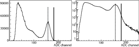
Figure 9: The spots in the spectrum which we use to get a relationship between ADC channel and deposited energy. The example spectrum is plotted twice, once in linear and once in logarithmic scale. The position of the elastic peak is shown by the dotted line, the so-called high-energy “edge”, which is defined as the inflection point at the right end of the logarithmic spectrum, is shown by the solid line.

Advantages and disadvantages of the usage of these two special locations in the spectra will be discussed below. First we describe how these positions are determined in the experimental spectra, which is a non-trivial task as for each five minute run 1022 energy spectra have to be analyzed and hence a fully automatic procedure is required.

3.2.1 Finding the peaks in the spectra

Figure 10: Energy spectrum with Gaussian filter applied (left) and its first derivative (right). The algorithm searches for the first zero crossing with negative slope starting from the upper end of the spectrum. This point indicates the position of the elastic peak in the ADC spectrum.

Mathematically, the elastic peak marks a local maximum in the energy spectrum and can be identified by a zero-crossing in the first derivative. Since there are no other maxima in the spectra at energies higher than the energy of elastically scattered electrons, the local maximum found at the highest energy indicates the position of the elastic peak. The procedure that determines this position is composed of three stages and is illustrated in fig. 10: first, a Gaussian filter is applied to the spectra with a sigma of two ADC channels. This prevents misidentification of statistical fluctuations or differential non-linearities of the ADC as a peak. Second, the first derivative is computed by subtracting the number of counts $N_{n}$ in the ADC channel $n$ from the number of counts $N_{n+1}$ in the ADC channel $n+1$, i.e. $N^{\prime}_{n}=N_{n+1}-N_{n}$, for $0\leq n\leq 254$. Third, the algorithm searches for the first zero crossing with negative slope in the derivative starting from the highest possible ADC value, $n=254$ (and then going down to lower ADC values). Normally, for a vast majority of calorimeter modules the positions of the elastic peaks are found reliably. However, if the calorimeter is not well calibrated, the peaks may be deformed to a shallow bump in the spectrum and the peak search may fail, the treatment of these cases are discussed in section 3.2.3.

3.2.2 Finding the edges in the spectra

Figure 11: Logarithm of an energy spectrum (left) and its second derivative (right). The indicated zero crossing in the second derivative marks the inflection point of the logarithmic spectrum which defines the position of the so-called high-energy “edge”.

As stated before, we define the so-called “edge” as the inflection point of the right shoulder in the logarithm of the spectrum (see fig. 11). If the right side of the elastic peak was perfectly Gaussian-shaped, there would be no inflection point in its logarithm at all, since the logarithm of a Gaussian is a parabola. However, the spectrum also contains a small amount of unrecognized pile-up events with energies that may sum up to values beyond the elastic peak. This results in an edge in the spectrum, at the location where the number of such pile-up events exceeds the number of elastically scattered electrons. The procedure to find the high-energy edge is similar to that for finding the peaks: First, the spectrum is smoothed, in this case by a median filter which is a rank filter with a window size of 11 ADC channels in our case. The advantage to use this kind of filter is that a median filter preserves the position of edges whereas a Gaussian filter preserves the position of the peaks. Next, the second derivative is computed and then the algorithm searches for the first zero crossing with positive slope starting from the upper end of the spectrum. Even if the calorimeter is in a completely uncalibrated state, the high-energy edges are found with 100% reliability.

3.2.3 Determining the position of the elastic peak

The position of the elastic peak together with the measured offset of the ADC spectrum gives sufficient information to relate the sum signal of the 3$\times$3 cluster of crystals to the known energy of the elastically scattered electron. Preferably this position is taken from the peak finding algorithm described in section 3.2.1. However, this peak search may fail if there are difficult conditions like:

• The calorimeter is in an uncalibrated state

• The module is located at an outer ring with only 5 neighbouring modules

• The module is operated at its high voltage limit

The general procedure is therefore to search both for the elastic peak and for the high-energy edge simultaneously. If both positions are found, the algorithm determines whether the distance between the peak and the edge is reasonable. This distance depends on the beam energy and the energy resolution of the cluster. If the distance exceeds specified limits, the peak determination is assumed to have failed. In this case — or if no peak is found — the peak position is estimated from the position of the high-energy edge.

3.3 Amplification factors of the individual modules

With the knowledge of the distribution parameters $\mu_{c}$, $\mu_{n}$ and $\mu_{d}$ one can write down an equation for the signal strength $S_{i}$ of each 3$\times$3 cluster $i$ caused by elastic events of energy $E_{0}$ depending on the amplification factors of the central crystal and its eight neighbours (see fig. 6):

$$S_{i}=[\mu_{c}k_{i_{0}}+\mu_{n}(k_{i_{1}}+k_{i_{3}}+k_{i_{5}}+k_{i_{7}})+\mu_{d}(k_{i_{2}}+k_{i_{4}}+k_{i_{6}}+k_{i_{8}})]E_{0}$$ (6)

where $k_{i_{j}}$ denotes the actual amplification factor of the members $0\leq j\leq 8$ of the 3$\times$3 cluster $i$, $1\leq i\leq 1022$. The numbering for $j$ follows the definition in fig. 6. Altogether there are 1022 equations for the 1022 3$\times$3 clusters of the calorimeter. Denoting from now on the amplification factor of module $i$ by $k_{i}$, one can write down 1022 equations for all 1022 clusters:

$$S_{1} = [\mu_{c}k_{1}+\mu_{n}(k_{2}+k_{8}+k_{1016})+\mu_{d}(k_{9}+k_{1017})]E_{0}$$

$$S_{2} = [\mu_{c}k_{2}+\mu_{n}(k_{1}+k_{3}+k_{9}+k_{1017})+\mu_{d}(k_{8}+k_{10}+k_{1016}+k_{1018})]E_{0}$$

$$\ S_{3} = [\mu_{c}k_{3}+\mu_{n}(k_{2}+k_{4}+k_{10}+k_{1018})+\mu_{d}(k_{9}+k_{11}+k_{1017}+k_{1019})]E_{0}$$

$$\dots$$

$$S_{1022} = [\mu_{c}k_{1022}+\mu_{n}(k_{7}+k_{1015}+k_{1021})+\mu_{d}(k_{6}+k_{1014})]E_{0}$$ (7)

Introducing the vectors $\vec{S}$ and $\vec{k}$,

$$\vec{S}=\begin{pmatrix}S_{1}\\ S_{2}\\ S_{3}\\ ..\\ S_{1022}\end{pmatrix}\,\,\,\,\,{\rm and}\,\,\,\,\,\vec{k}=\begin{pmatrix}k_{1}\\ k_{2}\\ k_{3}\\ ..\\ k_{1022}\end{pmatrix}$$ (8)

and the $1022\times 1022$ matrix ${\bf A}$,

$${\bf A}=\begin{pmatrix}\mu_{c}&\mu_{n}&0&0&0&0&0&\mu_{n}&\mu_{d}&...\\ \mu_{n}&\mu_{c}&\mu_{n}&0&0&0&0&\mu_{d}&\mu_{n}&...\\ 0&\mu_{n}&\mu_{c}&\mu_{n}&0&0&0&0&\mu_{d}&...\\ 0&0&\mu_{n}&\mu_{c}&\mu_{n}&0&0&0&0&...\\ 0&0&0&\mu_{n}&\mu_{c}&\mu_{c}&\mu_{n}&0&0&...\\ {10}\\ 0&0&0&0&0&\mu_{d}&\mu_{n}&0&0&...\end{pmatrix}$$ (9)

the system of linear equations can be written in matrix form

$$\vec{S}={\bf A}\vec{k}E_{0}$$ (10)

By matrix inversion of ${\bf A}$ the individual amplification factors $k_{i}$ of all calorimeter modules can now be calculated:

$$\vec{k}=\frac{1}{E_{0}}{\bf A}^{-1}\vec{S}$$ (11)

The inversion of a 1022$\times$1022-matrix requires usually a lot of computation time. It is done here using a numerical method which benefits from the fact that the matrix has non-zero elements only close to its main diagonal. The values of the elements of the inverted matrix which are calculated this way differ by less than one percent from those using no approximation. The matrix ${\bf A}$ needs to be adapted to the actual situation of the calorimeter. If, for example, the calorimeter channel $j$ is out of order due to a technical problem, its high voltage is set to zero and this individual channel does not contribute to the sum signal of its neighbours. This can easily be taken into account by setting all members of the $j$th row and $j$th column in the matrix to zero except for the diagonal element ($j$,$j$) which is set to 1, i.e. channel $j$ is completely decoupled from the neighbouring modules.

3.4 Adjusting the amplification factors

The channels are calibrated by adjusting the high voltages of the photomultipliers. The charge $Q_{i}$ for a fixed number of incident photons at the photocathode is a power function of the applied voltage $U$:

$$Q_{i}=\alpha_{i}U^{\beta_{i}}$$ (12)

Having determined the current amplification factor $k_{i}$ of channel $i$ using eq. 11, one can calculate the new voltage $U_{i}^{new}$ to reach the desired amplification factor $k_{demand}$:

$$U_{i}^{new}=\sqrt[\beta_{i}]{\frac{k_{demand}}{k_{i}}}U_{i}^{old}$$ (13)

The proportionality factor $\alpha_{i}$ cancels out when calculating new voltages, so only the amplification exponent $\beta_{i}$ is of interest. Several tubes have been tested using a pulsed blue LED. The measured pulse heights as a function of the applied high voltage are shown in fig. 12. The proportionality between pulse height and charge $Q$ was assumed.

Figure 12: Pulse heights of four different photomultiplier tubes as a function of the applied high voltage in logarithmic scale. From the slope of the straight line one can derive the parameter $\beta$, in this case $6.48\leq\beta\leq 7.39$.

Due to the large number of photomultipliers, not all $\beta_{i}$ have been individually determined. Approximate values were provided by the manufacturer. An average value of $\beta_{0}=7.0$ is used which means that the error $\Delta\beta_{i}$ in the amplification exponent is of the order $\pm 0.5$. For $\beta_{i}\neq 7.0$ the new voltage $U_{i}^{new}$ is rather an approximation than the exactly desired value and the calibration has to be iterated to reach the desired charge $Q_{nom}$. It can be shown mathematically that the procedure converges as long as the true $\beta_{i}\leq 1.5\cdot\beta_{0}$: let $\Delta\beta$ the deviation of the the true parameter $\beta_{i}$ from $\beta_{0}$, i.e.

$$\beta_{i}=\beta_{0}+\Delta\beta$$ (14)

Since $Q_{i}$ is proportional to $k_{i}$, we get for the new voltage $U_{i}^{new}$:

$$U_{i}^{new}=\sqrt[\beta_{i}-\Delta\beta]{\frac{Q_{nom}}{Q_{i}^{old}}}U_{i}^{old}$$ (15)

Using eq. 12, one gets the new charge

$$Q_{i}^{new}=\alpha_{i}\left(\frac{Q_{nom}}{Q_{i}^{old}}\right)^{\frac{\beta_{i}}{\beta_{i}-\Delta\beta}}(U_{i}^{old})^{\beta_{i}}=\left(\frac{Q_{nom}}{Q_{i}^{old}}\right)^{\frac{1}{1-\frac{\Delta\beta}{\beta_{i}}}}Q_{i}^{old}$$ (16)

With the abbreviation

$$\gamma=\frac{\Delta\beta}{\beta_{i}}$$ (17)

we can rewrite eq.(16):

$$Q_{i}^{new}=(Q_{nom})^{\frac{1}{1-\gamma}}\left(Q_{i}^{old}\right)^{\frac{-\gamma}{1-\gamma}}$$ (18)

Division by $Q_{nom}$ yields

$$\frac{Q_{i}^{new}}{Q_{nom}}=\left(\frac{Q_{nom}}{Q_{i}^{old}}\right)^{\frac{\gamma}{1-\gamma}}$$ (19)

From eq. 19 follows that the calculation of new voltages converges as long as

$$|\frac{\gamma}{1-\gamma}|<1$$ (20)

Hence, the convergence constraint for $\gamma$ and $\Delta\beta$ respectively is:

$$\gamma<\frac{1}{2}\quad\Leftrightarrow\quad\Delta\beta<\frac{1}{2}\beta_{i}$$ (21)

The condition $\Delta\beta<\frac{1}{2}\beta_{i}$ means in our case that as long as $\Delta\beta<3.5$, the procedure still converges. This requirement is very well fulfilled since for our photomultipliers $\,\,-\frac{1}{2}<\Delta\beta<+\frac{1}{2}$, so one can expect a fast convergence.

4 Measurements and results

Since the setup of the PbF₂ calorimeter in 2000, the calibration procedure has been successfully used during 8000 hours of beam. In this section, some of the benefits and properties will be presented.

4.1 Calibration starting from an uncalibrated state

To test the calibration procedure, the calorimeter was brought in an uncalibrated state by applying random high voltages within the allowed limits to all modules. An amplification factor $k_{nom}$ was demanded so that the elastic peak lies at ADC channel 170 above pedestals. In this case, three steps were sufficient to bring the calorimeter into a well-calibrated state. Fig. 13 shows 3$\times$3 sum spectra before and after calibration. One can clearly see the enhancement in energy resolution and uniformity of the energy spectra.

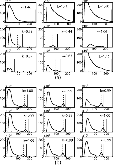
Figure 13: Energy spectra of 3$\times$3 crystal clusters in uncalibrated state (a) and after calibration (b). The positions of the high energy edge that were found by the algorithm are indicated by the solid lines. The positions of the elastic peak — if found by the algorithm — are indicated by the dashed lines. The normalized amplification factors $k=k_{i}/k_{nom}$ for each module are denoted in the graphs. After three calibration steps the spectra get more uniform and the elastic peaks become more prominent.

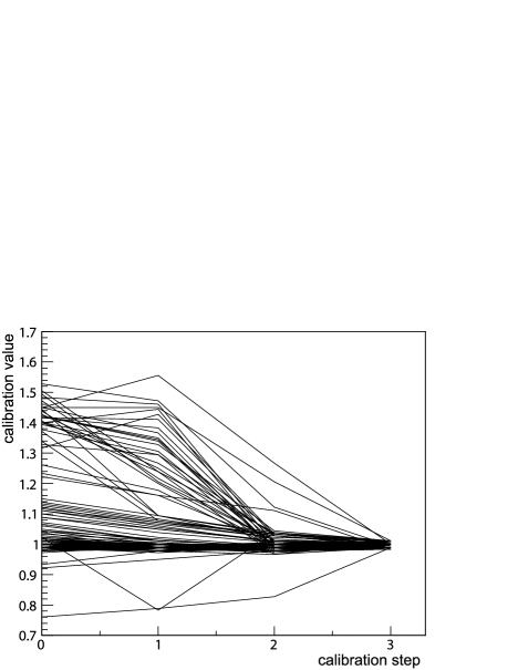
Figure 14: Normalized amplification factors $k$ of selected single modules and their development during the calibration procedure. After three calibration steps the mean calibration value changed from 1.02 to 1.00, the standard deviation decreased from 0.11 to 0.01.

Fig. 14 shows how the normalized amplification factors $k=k_{i}/k_{nom}$ of the single modules evolve during the calibration procedure. A normalized amplification factor of $k_{i}=1$ means that channel $i$ is perfectly calibrated. After three calibration steps the mean calibration value changed from $\bar{k}=1.02$ to $\bar{k}=1.00$, the standard deviation decreased from 0.11 to 0.01.

4.2 Energy resolution of the PbF₂ calorimeter

To quantify the energy resolution of the calorimeter, we use the width of the elastic peaks in the measured energy spectra. The observed peak width depends on various factors, like the variation of the scattered electron energy within the acceptance, energy straggling of the electrons within the hydrogen target and the material between target and calorimeter crystals, or the intrinsic energy resolution of the detector material itself.

This observed relative energy resolution is determined by fitting a phenomenological function to the elastic peak of the energy spectra [14] which takes into account the radiative tail and the shower leakages. The function describes the peak with a Gaussian with mean $\mu$ and width $\sigma_{R}$ for the high energy side and a Gaussian with mean $\mu$ and width $\sigma_{L}$ modified by an exponential for the low energy side:

$$f(x)=\left\{\begin{array}[]{l l r}C\cdot\left\{\exp\left[-\frac{1}{2}\left(\frac{x-\mu}{\sigma_{L}}\right)^{2}\right]+\exp\left[\frac{x-\mu}{\lambda}\right]\cdot\left(1-\exp\left[-\frac{1}{2}\left(\frac{x-\mu}{\sigma_{L}}\right)^{2}\right]\right)\right\}&\mathrm{,}&x<\mu\\ C\cdot\exp\left[-\frac{1}{2}\left(\frac{x-\mu}{\sigma_{R}}\right)^{2}\right]&\mathrm{,}&x\geq\mu\end{array}\right.$$ (22)

The relative energy resolution $\Delta E/E$ is defined here as $\sigma_{R}/\mu$. Because the signals of nine neighbouring channels are summed up, the calibration enhances the energy resolution. For the calibration example presented in the previous section, the average effective resolution improved from $13.9\%$ before calibration to $5.0\%$ after calibration.

4.3 Stability of the calibration and routine operation

Once a calibrated state has been reached, the calorimeter remains calibrated for several hours. In order to test the stability, we left the high voltage of the multipliers unchanged during a measurement period of 24 h and observed only small decalibration effects. This is possible because of the stable experimental conditions: the temperature in the experimental halls is kept stable to $\Delta T=\pm 1^{\circ}$C, the beam current is stabilized on the $10^{-6}$ level and hence the rates on the detector are very stable. The main source of decalibration is the response of the PbF₂ crystals to the high radiation level to which they are exposed. Radiation damages in the crystals lead to the formation of color centers and thus to a loss of light yield which is specific to each crystal. The calibration procedure compensates for this effect by increasing the high voltages of the photomultiplier tubes and is applied once per hour. During a beam period of three weeks, the average high voltage is increased by about 25 V. After a data taking period (typically two weeks), optical bleaching is applied to the crystals [13] and most of the radiation damages are repaired. The average HV at the beginning of the following beam time is then lowered again, as shown in fig. 15,

Figure 15: Average PMT high voltage of the calorimeter versus run number. The graph covers four beam times where one can see an increase of the voltage with time because of the radiation damage in the PbF₂ crystals. After each beam time the radiation damage is reduced by exposing the crystals to blue light thus reducing the necessary HV again.

where the mean voltage of the calorimeter channels is shown as a function of the run number. Ten runs correspond to one hour of data taking. One can see four periods of data taking, each of them 2–3 weeks long. The high voltages start at low values and are increased automatically by the calibration procedure to compensate for the radiation damage.
Using massive parallelization and high-speed network equipment, the interval between runs needed for readout, storage and preparation of the next run was reduced to 30 s, resulting in a data taking efficiency of 90%. The calibration procedure described here can be partly performed during data taking, applying the new high voltages can be done in the time window between two runs without compromising the efficiency.

5 Summary

A calibration procedure was developed for a segmented, total absorbing homogenous electromagnetic calorimeter consisting of 1022 lead fluoride crystals. Since the signals of 3$\times$3 neighbouring modules are summed up and digitized to determine the energy of a single event, a uniform gain in all modules is a prerequisite for a good effective energy resolution. In order to achieve this, the photomultipliers were precalibrated before they were installed in the calorimeter. For the analog summation circuit high precision components such as resistors with 0.1% tolerance and capacitors with 1% tolerance were used. A uniform gain is then obtained by the calibration procedure that was presented here. Three conditions had to be fulfilled: first, the large number of channels required a fully automatic, reliable treatment. Second, since only the sum signals are available with sufficient digital resolution, the amplification factors of the single modules had to be extracted from the sum signal. And third, the method had to tolerate ignorance of the precise gain coefficients of the PMTs.

The first issue was addressed by implementing a combined search for the elastic peak and the so-called high-energy “edge” in the energy spectra which ensures that the calibration state of the 3$\times$3-clusters is always correctly determined. For the second issue a mathematical solution was found by forming a set of 1022 linear equations and solving them by inverting a 1022$\times$1022 matrix. For the third issue it could be proven that the exact knowledge of the individual exponential gain factors $\beta$ of the photomultipliers is not necessary as long as the true gain factor of a multiplier does not exceed the average gain factor which is used for the calculation of the voltages by more than a factor of 1.5.

The calibration procedure has been in use for several years now. More than $10^{8}$ energy spectra measured at beam energies from 300 MeV up to 1500 MeV have been successfully analyzed. The calorimeter can be brought from an uncalibrated to a well-calibrated state within three calibration steps corresponding to 10 minutes real time. The energy resolution is significantly enhanced within these three calibration steps and can be kept at the same level by applying a new calibration step once an hour.

6 Acknowledgements

This work was supported by the Deutsche Forschungsgemeinschaft in the framework of the CRC 201, 443 and the SPP 1034. We would like to thank the crew of the MAMI accelerator for providing us with an excellent electron beam.

References

- [1] Maas, F. E. et al.: Phys. Rev. Lett.93 (2004) 022002
- [2] Maas, F. E. et al.: Phys. Rev. Lett.94 (2005) 152001
- [3] Maas, F. E. et al.: Phys. Rev. Lett.94 (2005) 082001
- [4] Baunack, S. et al.: Phys. Rev. Lett.102 (2009) 151803
- [5] Abdullin, S. et al.: Eur. Phys. J. C55 (2008) 159-171
- [6] Ambrosino, F. et al.: Nucl. Instr. and Meth. A598 (2009) 239-243
- [7] Abachi, S. et al.: Nucl. Instr. and Meth. A338 (1994) 185-253
- [8] Achenbach, P.et al.: Nucl. Instrum. Meth. A465 (2001) 318-328
- [9] Köbis, S. et al..: Nucl. Phys. Proc. Suppl. 61 B (1998), 625-629
- [10] Kothe, R.: Ph.D. thesis, Mainz University (2008)
- [11] Bianchi, E.: Nucl. Instr. and Meth. A279 (1989) 473-478
- [12] Grimm:, K: Diploma thesis, Universität Mainz (1996)
- [13] Achenbach, P.et al.: Nucl. Instrum. Meth. A416 (1998) 357-363
- [14] Matulewicz, T. et al., Nucl. Instrum. Meth. A289 (1990) 194-204