On minimising automata with errors

Abstract

The problem of $k$-minimisation for a DFA $M$ is the computation of a smallest DFA $N$ (where the size $\lvert M\rvert$ of a DFA $M$ is the size of the domain of the transition function) such that $L(M)\mathop{\bigtriangleup}L(N)\subseteq\Sigma^{<k}$, which means that their recognized languages differ only on words of length less than $k$. The previously best algorithm, which runs in time $\mathcal{O}(\lvert M\rvert\log^{2}n)$ where $n$ is the number of states, is extended to DFAs with partial transition functions. Moreover, a faster $\mathcal{O}(\lvert M\rvert\log n)$ algorithm for DFAs that recognise finite languages is presented. In comparison to the previous algorithm for total DFAs, the new algorithm is much simpler and allows the calculation of a $k$-minimal DFA for each $k$ in parallel. Secondly, it is demonstrated that calculating the least number of introduced errors is hard: Given a DFA $M$ and numbers $k$ and $m$, it is NP-hard to decide whether there exists a $k$-minimal DFA $N$ with $\lvert L(M)\mathop{\bigtriangleup}L(N)\rvert\leq m$. A similar result holds for hyper-minimisation of DFAs in general: Given a DFA $M$ and numbers $s$ and $m$, it is NP-hard to decide whether there exists a DFA $N$ with at most $s$ states such that $\lvert L(M)\mathop{\bigtriangleup}L(N)\rvert\leq m$.

1 Introduction

Deterministic finite automata (DFAs) are one of the simplest devices recognising languages. The study of their properties is motivated by (i) their simplicity, which yields efficient operations, (ii) their wide-spread applications, (iii) their connections to various other areas in theoretical computer science, and (iv) the apparent beauty of their theory. A DFA $M$ is a quintuple ${\langle Q,\Sigma,\delta,q_{0},F\rangle}$, where $Q$ is its finite state-set, $\Sigma$ is its finite alphabet, $\delta\colon Q\times\Sigma\to Q$ is its partial transition function, $q_{0}\in Q$ is its starting state, and $F\subseteq Q$ is its set of accepting states. The DFA $M$ is total if $\delta$ is total. The transition function $\delta$ is extended to $\delta\colon Q\times\Sigma^{*}\to Q$ in the standard way. The language $L(M)$ that is recognised by the DFA $M$ is $L(M)=\{w\>|\>\delta(q_{0},w)\in F\}$.

Two DFAs $M$ and $N$ are equivalent (written as $M\equiv N$) if $L(M)=L(N)$. A DFA $M$ is minimal if all equivalent DFAs are larger. One of the classical DFA problems is the minimisation problem, which given a DFA $M$ asks for the (unique) minimal equivalent DFA. The asymptotically fastest DFA minimisation algorithm runs in time $\mathcal{O}(\lvert\Sigma\rvert\,n\log n)$ and is due to Hopcroft [9, 7], where $n=\lvert Q\rvert$; its variant for partial DFAs is known to run in time $\mathcal{O}(\lvert M\rvert\log n)$.

Recently, minimisation was also considered for hyper-equivalence [2, 3], which allows a finite difference in the languages. Two languages $L$ and $L^{\prime}$ are hyper-equivalent if $\lvert L\mathop{\bigtriangleup}L^{\prime}\rvert<\infty$, where $\mathop{\bigtriangleup}$ denotes the symmetric difference of two sets. The DFAs $M$ and $N$ are hyper-equivalent if their recognised languages are. The DFA $M$ is hyper-minimal if all hyper-equivalent DFAs are larger. The algorithms for hyper-minimisation [3, 2] were gradually improved over time to the currently best run-time $\mathcal{O}(\lvert M\rvert\log^{2}n)$ [8, 6], which can be reduced to $\mathcal{O}(\lvert M\rvert\log n)$ using a strong computational model (with randomisation or special memory access). Since classical DFA minimisation linearly reduces to hyper-minimisation [8], an algorithm that is faster than $\mathcal{O}(\lvert M\rvert\log n)$ seems unlikely. Moreover, according to the authors’ knowledge, randomisation does not help Hopcroft’s [5] or any other DFA minimisation algorithm. Thus, the randomised hyper-minimisation algorithm also seems to be hard to improve.

Already [3] introduces a stricter notion of hyper-equivalence. Two languages $L$ and $L^{\prime}$ are $k$-similar if they only differ on words of length less than $k$. Analogously, DFAs are $k$-similar if their recognised languages are. A DFA $M$ is $k$-minimal if all $k$-similar DFAs are larger, and the $k$-minimisation problem asks for a $k$-minimal DFA that is $k$-similar to the given DFA $M$. The known algorithm [6] for $k$-minimisation of total DFAs runs in time $\mathcal{O}(\lvert M\rvert\log^{2}n)$, however it is quite complicated and fails for non-total DFAs.

In this contribution, we present a simpler $k$-minimisation algorithm for general DFAs, which still runs in time $\mathcal{O}(\lvert M\rvert\log^{2}n)$. This represents a significant improvement compared to the complexity for the corresponding total DFA if the transition table of $M$ is sparse. Its running time can be reduced if we allow a stronger computational model. In addition, the new algorithm runs in time $\mathcal{O}(\lvert M\rvert\log n)$ for every DFA $M$ that recognises a finite language. Finally, the new algorithm can calculate (a compact representation of) a $k$-minimal DFA for each possible $k$ in a single run (in the aforementioned run-time). Outputting all the resulting DFAs might take time $\Omega(n\lvert M\rvert\log^{2}n)$.

Although $k$-minimisation can be efficiently performed, no uniform bound on the number of introduced errors is provided. In the case of hyper-minimisation, it is known [10] that the optimal (i.e., the DFA committing the least number of errors) hyper-minimal DFA and the number of its errors $m$ can be efficiently computed. However, this approach does not generalise to $k$-minimisation. We show that this is for a reason: already the problem of calculating the number $m$ of errors of an optimal $k$-minimal automaton is NP-hard.

Finally, for some applications it would be beneficial if we could balance the number $m$ of errors against the compression rate $\frac{\lvert N\rvert}{\lvert M\rvert}$. Thus, we also consider the question whether given a DFA $M$ and two integers $s$ and $m$ there is a DFA $N$ with at most $s$ states that commits at most $m$ errors (i.e., $\lvert L(M)\mathop{\bigtriangleup}L(N)\rvert\leq m$). Unfortunately, we show that this problem is also NP-hard.

2 Preliminaries

We usually use the two DFAs $M={\langle Q,\Sigma,\delta,q_{0},F\rangle}$ and $N=\langle P,\Sigma,\mu,p_{0},F^{\prime}\rangle$. We also write $\delta(w)$ for $\delta(q_{0},w)$. The right-language $L_{M}(q)$ of a state $q\in Q$ is the language $L_{M}(q)=\{w\>|\>\delta(q,w)\in F\}$ recognised by $M$ starting in state $q$. Minimisation of DFAs is based on calculating the equivalence $\equiv$ between states, which is defined by $q\equiv p$ if and only if $L_{M}(q)=L_{N}(p)$. Similarly, the left language of $q$ is the language $\delta^{-1}(q)=\{w\>|\>\delta(w)=q\}$ of words leading to $q$ in $M$.

For two languages $L$ and $L^{\prime}$, we define their distance $d(L,L^{\prime})$ as

$$d(L,L^{\prime})=\min{}\{\ell\>|\>L\cap\Sigma^{\geq\ell}=L^{\prime}\cap\Sigma^{\geq\ell}\}\enspace,$$

where $\min{}\emptyset=\infty$. Actually, $d$ is an ultrametric. The distance $d$ can be extended to states: $d(q,p)=d(L_{M}(q),L_{N}(p))$ for $q\in Q$ and $p\in P$. It satisfies the simple recursive formula:

$$d(q,p)=\begin{cases}0&\text{ if }q\equiv p,\\ 1+\max{}\{d(\delta(q,a),\mu(p,a))\>|\>a\in\Sigma\}&\text{ otherwise}.\end{cases}$$ (1)

Since $d$ is an ultrametric on languages, (1) yields that the distance $d(q_{1},q_{2})$ between $q_{1},q_{2}\in Q$ in the DFA $M$ is either infinite or small. Formally, $d(q_{1},q_{2})=\infty$ or $d(q_{1},q_{2})<\lvert Q\rvert$.

The minimal DFAs considered in this paper are obtained mostly by state merging. We say that the DFA $N$ is the result of merging state $q$ to state $p$ (assuming $q\neq p$) in $M$ if $N$ is obtained from $M$ by changing all transitions ending in $q$ to transitions ending in $p$ and deleting the state $q$. If $q$ was the starting state, then $p$ is the new starting state. Formally, $P=Q\setminus\{q\}$, $F^{\prime}=F\setminus\{q\}$, and

$$\mu(r,a) =\begin{cases}p&\text{if }\delta(r,a)=q\\ \delta(r,a)&\text{otherwise,}\end{cases} p_{0} =\begin{cases}p&\text{if }q_{0}=q\\ q_{0}&\text{otherwise.}\end{cases}$$

The process is illustrated in Fig. 1.

Figure 1: Merging state $G$ into $I$.

Finally, let ${\mathop{in\text{-}level}\nolimits}_{M}(q)$ be the length of the longest word leading to $q$ in $M$. If there is no such longest word, then ${\mathop{in\text{-}level}\nolimits}_{M}(q)=\infty$. Formally, ${\mathop{in\text{-}level}\nolimits}_{M}(q)=\sup{}\{\lvert w\rvert\>|\>w\in\delta^{-1}(q)\}$ for every $q\in Q$. The structural characterisation of hyper-minimal DFAs [3, Sect. 3.2] relies on a state classification into kernel and preamble states. The set $\operatorname{Ker}(M)$ of kernel states consists of all states $q\in Q$ with ${\mathop{in\text{-}level}\nolimits}_{M}(q)=\infty$, whereas the remaining states are preamble states. Roughly speaking, the kernels of two hyper-equivalent and hyper-minimal automata are isomorphic in the standard sense, and their preambles are also isomorphic except for acceptance values.

3 Efficient $k$-minimisation

3.1 $k$-similarity and $k$-minimisation

Two languages $L$ and $L^{\prime}$ are $k$-similar if they only differ on words of length smaller than $k$, and the two DFAs $M$ and $N$ are $k$-similar if their recognised languages are. The DFA $M$ is $k$-minimal if all $k$-similar DFAs are larger. In this section, we first give a general simple algorithm $k$-Minimise that computes a $k$-minimal DFA that is $k$-similar to the input DFA $M$. Then we present a data structure that allows a fast, yet simple implementation of this algorithm.

Definition 1

For two languages $L$ and $L^{\prime}$, we let $L\sim_{k}L^{\prime}\iff d(L,L^{\prime})\leq k$.

The hyper-equivalence relation [3] can be now defined as $\mathord{\sim}=\bigcup_{k}\mathord{\sim_{k}}$. Next, we extend $k$-similarity to states.

Definition 2

Two states $q\in Q$ and $p\in P$ are $k$-similar, denoted by $q\sim_{k}p$, if

$$d(q,p)+\min(k,{\mathop{in\text{-}level}\nolimits}_{M}(q),{\mathop{in\text{-}level}\nolimits}_{N}(p))\leq k\enspace.$$

While $\sim_{k}$ is an equivalence relation on languages, it is, in general, only a compatibility relation (i.e., reflexive and symmetric) on states. On states the hyper-equivalence is not a direct generalisation of $k$-similarity. Instead, $p\sim q$ if and only if $L_{M}(q)\sim L_{N}(p)$. We use the $k$-similarity relation to give a simple algorithm $\textnormal{$k$-Minimise}(M)$, which constructs a $k$-minimal DFA (see Algorithm 1). In Section 3.2 we show how to implement it efficiently.

Algorithm 1 $\textnormal{$k$-Minimise}(M)$ with minimal $M$

1:calculate ${\sim_{k}}$ on $Q$

2:$N\leftarrow M$

3:while $q\sim_{k}p$ for some $q,p\in P$ and $q\neq p$ do

4:     if ${\mathop{in\text{-}level}\nolimits}_{M}(q)\geq{\mathop{in\text{-}level}\nolimits}_{M}(p)$ then

5:         swap $q$ and $p$      

6:     $N\leftarrow\textnormal{Merge}(N,q,p)$

Theorem 3.1

$k$-Minimise returns a $k$-minimal DFA that is $k$-similar to $M$.

3.2 Distance forests

In this section we define distance forests, which capture the information of the distance between states of a given minimal DFA $M$. We show that $k$-minimisation can be performed in linear time, when a distance forest for $M$ is supplied. We start with a total DFA $M$ because in this case the construction is fairly easy. In Section 3.3 we show how to extend the construction to non-total DFAs.

Let $\mathcal{F}$ be a forest (i.e., set of trees) whose leaves are enumerated by $Q$ and whose edges are weighted by elements of $\mathbb{N}$. For convenience, we identify the leaf vertices with their label. For every $q\in Q$, we let $\mathrm{tree}(q)\in\mathcal{F}$ be the (unique) tree that contains $q$. The level $\operatorname{level}(v)$ of a vertex $v$ in $t\in\mathcal{F}$ is the maximal weight of all paths from $v$ to a leaf, where the weights are added along a path. Finally, given two vertices $v_{1},v_{2}$ of the same tree $t\in\mathcal{F}$, the lowest common ancestor of $v_{1}$ and $v_{2}$ is the vertex $\operatorname{lca}(v_{1},v_{2})$.

Definition 3 (Distance forest)

Let $\mathcal{F}$ be a forest whose leaves are enumerated by $Q$. Then $\mathcal{F}$ is a distance forest for $M$ if for every $q,p\in Q$ we have

$$d(q,p)=\begin{cases}\operatorname{level}(\operatorname{lca}(q,p))&\text{ if }\mathrm{tree}(q)=\mathrm{tree}(p),\\ \infty&\text{ otherwise}.\end{cases}$$

Figure 2: A distance forest for the left DFA of Fig. 1. Single-node trees are omitted.

In order to construct a distance forest we use (1) to calculate the distance. Mind that $M$ is minimal, so there are no states with distance $0$. In phase $\ell$, we merge all states at distance exactly $\ell$ into one state. Since we merged all states of distance at most $\ell-1$ in the previous phases, we only need to identify the states of distance $1$ in the merged DFA. Thus we simply group the states according to their vectors of transitions by letters from $\Sigma=\{a_{1},\dotsc,a_{m}\}$. To this end we store these vectors in a dictionary, organised as a trie of depth $m$. The leaf of a trie corresponding to a path $(q_{1},\dotsc,q_{m})$ keeps a list of all states $q$ such that $\delta(q,a_{i})=q_{i}$ for every $1\leq i\leq m$. For each node $v$ in the trie we keep a linear dictionary that maps a state $q$ into a child of $v$. We demand that this linear dictionary supports search, insertion, deletion, and enumeration of all elements.

Theorem 3.2

Given a total DFA $M$, we can build a distance forest for $M$ using $\mathcal{O}(\lvert M\rvert\log n)$ linear-dictionary operations.

We now shortly discuss some possible implementations of the linear dictionary. An implementation using balanced trees would have linear space consumption and the essential operations would run in time $\mathcal{O}(\log n)$. If we allow randomisation, then we can use dynamic hashing. It has a worst-case constant time look-up and an amortised expected constant time for updates [11]. Since it is natural to assume that $\log n$ is proportional to the size of a machine word, we can hash in constant time. We can obtain even better time bounds by turning to more powerful models. In the RAM model, we can use exponential search trees [1], whose time per operation is $\mathcal{O}(\frac{(\log\log n)^{2}}{\log\log\log n})$ in linear space. Finally, if we allow a quadratic space consumption, which is still possible in sub-quadratic time, then we can allocate (but not initialise) a table of size $\lvert M\rvert\times n$. Standard methods can be used to keep track of the actually used table entries, so that we obtain a constant run-time for each operation, but at the expense of $\Theta(\lvert M\rvert\,n)$ space; i.e., quadratic memory consumption.

We can now use a distance forest to efficiently implement $k$-Minimise. For each state $q$ we locate its highest ancestor $v_{q}$ with $\operatorname{level}(v_{q})\leq k-{\mathop{in\text{-}level}\nolimits}(q)$. Then $q$ can be merged into any state that occurs in the subtree rooted in $v_{q}$ (assuming it has a smaller ${\mathop{in\text{-}level}\nolimits}$). This can be done using a depth-first traversal on the trees of the distance forest. A more elaborate construction based on this approach yields the following.

Theorem 3.3

Given a distance forest for $M$, we can compute the size of a $k$-minimal DFA that is $k$-similar to $M$ for all $k$ in time $\mathcal{O}(\lvert M\rvert)$. For a fixed $k$, we can also compute a $k$-minimal DFA in time $\mathcal{O}(\lvert M\rvert)$. Finally, we can run the algorithm in time $\mathcal{O}(\lvert M\rvert\log n)$ such that it has a $k$-minimal DFA stored in memory in its $k$-th phase.

3.3 Finite languages and partial transition functions

The construction of a distance forest was based on a total transition function $\delta$, and the run-time was bounded by the size of $\delta$. We now show a modification for the non-total case. The main obstacle is the construction of a distance forest for an acyclic DFA. The remaining changes are relatively straightforward.

Theorem 3.4

For every acyclic DFA $M$ we can build a distance forest in time $\mathcal{O}(\lvert M\rvert\log n)$.

Proof (sketch)

Since $L(M)$ is finite, we have that $m(p)=\max{}\{\lvert w\rvert\>|\>w\in L_{M}(p)\}$ is a natural number for every state $p$. Let $Q_{i}=\{p\>|\>m(p)=i\}$ and $Q_{<\infty}=\bigcup_{i}Q_{i}$. Every state has a finite right-language, and thus every distance forest consists of a single tree. We iteratively construct the fragments of this tree by starting from a single leaf $\bot$, which represents the empty language and “undefinedness” of the transition function. Before we start to process $Q_{t}$, we have already constructed the distance tree for $\bigcup_{i<t}Q_{i}$. The constructed fragments are connected to a single path, called the spine, which ends at the leaf $\bot$ (see Fig. 3).

Let $Q_{t}=\{p_{1},\dotsc,p_{s}\}$, and let $v\in Q_{t}$. Moreover, let $\operatorname{f}(v)$ be the vector of states ${\bf v}=(\delta(v,a))_{a\in\Sigma}$, where the coordinates are sorted by a fixed order on $\Sigma$. Define the distance between those vectors as

$$d((p_{a})_{a\in\Sigma},(p^{\prime}_{a})_{a\in\Sigma})=\max{}\{d(p_{i},p^{\prime}_{i})+1\>|\>a\in\Sigma\}\enspace,$$

where we know that $d(p_{i},\bot)=m(p_{i})$ and $d(\bot,p^{\prime}_{i})=m(p^{\prime}_{i})$. Similarly to the distance, we can define the father $\operatorname{f}({\bf v})$ of a vector ${\bf v}=(p_{a})_{a\in\Sigma}$ as $\operatorname{f}({\bf v})=(\operatorname{f}(p_{a}))_{a\in\Sigma}$. Then

$$\operatorname{f}^{\ell+1}(v)=\operatorname{f}^{\ell+1}(v^{\prime})\iff\operatorname{f}^{\ell}({\bf v})=\operatorname{f}^{\ell}({\bf v^{\prime}}).$$

We can now use a divide-and-conquer approach: First, for each vector we calculate its $2^{k}$-th ancestor, where $k=\lceil\log s/2\rceil$. Then all such vectors are sorted according to their ancestors, in particular they are partitioned into blocks with the same ancestors. After that we recurse onto those (bottom) blocks that have more than two entries and onto the upper block, which consists of the different $2^{k}$-ancestors. The recursion ends for blocks containing at most two vectors, for which we calculate the distance tree directly. ∎

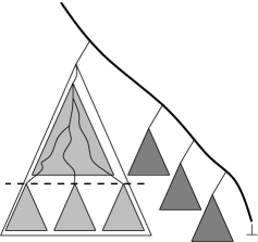
Figure 3: Illustration for the construction of the distance tree. The spine is depicted using with a thicker line. Splitting one fragment into smaller recursive calls is shown.

For every state $q\in Q$, its signature $\operatorname{{sig}}(q)$ is $\{a\>|\>L_{M}(\delta(q,a))\text{ is infinite}\}$. If $\operatorname{{sig}}(q)\neq\operatorname{{sig}}(p)$, then $d(q,p)=\infty$, which allows us to keep a separate dictionary for each signature. Let us fix such a trie. To take into account also the transitions by letters outside the signature, we introduce a fresh letter $\$$, whose transitions are represented in the trie as well. We organize them such that in phase $\ell$ the $\$$-transitions for the states $q$ and $p$ are the same if and only if $\max{}\{d(\delta(q,a),\delta(p,a))\>|\>a\notin\operatorname{{sig}}(q)\}\leq\ell-1$. This is easily organised if the distance forest for all states with a finite right-language is supplied.

Theorem 3.5

Given a (non-total) DFA $M$ we can build a distance forest for it using $\mathcal{O}(\lvert M\rvert\log n)$ linear-dictionary operations.

4 Hyper-equivalence and hyper-minimisation

When considering minimisation with errors, it is natural that one would like to impose a bound on the total number of errors introduced by minimisation. In this section, we investigate whether given $m,s\in\mathbb{N}$ and a DFA $M$ we can construct a DFA $N$ such that:

1. $N$ is hyper-equivalent to $M$; i.e., $N\sim M$,

2. $N$ has at most $s$ states, and

3. $N$ commits at most $m$ errors compared to $M$; i.e., $\lvert L(N)\mathop{\bigtriangleup}L(M)\rvert\leq m$.

Let us call the general problem ‘error-bounded hyper-minimisation’. We show that this problem is intractable (NP-hard). Only having a bound on the number of errors allows us to return the original DFA, which commits no errors.

To show NP-hardness of the problem we reduce the 3-colouring problem to it. Roughly speaking, we construct the DFA $M$ from a graph $G=\langle V,E\rangle$ as follows. Each vertex $v\in V$ is represented by a state $v\in Q$, and each edge $e\in E$ is represented by a symbol $e\in\Sigma$. We introduce additional states in a way such that their isomorphic copies are present in any minimal DFA that is hyper-equivalent to $M$. The additional states are needed to ensure that for every edge $e=\{v_{1},v_{2}\}\in E$ the languages $L_{M}(\delta(v_{1},e))$ and $L_{M}(\delta(v_{2},e))$ differ. Now we assume that $m=\lvert E\rvert\cdot(\lvert V\rvert-2)$ and $s=14$. We construct the DFA $M$ such that all vertices of $V\subseteq Q$ are hyper-equivalent to each other and none is hyper-equivalent to any other state. We can save $\lvert V\rvert-3$ states by merging all states of $V$ into at most $3$ states. These merges will cause at least $\lvert E\rvert\cdot(\lvert V\rvert-2)$ errors. Additionally, $3$ states will become superfluous after the merges, so that we can save $\lvert V\rvert$ states. There are two cases:

• If the input graph $G$ is $3$-colourable by $c\colon V\to[3]$, then we can merge all states of $c^{-1}(i)$ into a single state for every $i\in[3]$. Since $c$ is proper, we never merge states $v_{1},v_{2}\in Q$ with $\{v_{1},v_{2}\}\in E$, which avoids further errors.

• On the other hand, if $G$ is not $3$-colourable, then we merge at least two states $v_{1},v_{2}\in Q$ such that $e=\{v_{1},v_{2}\}\in E$. This merge additionally introduces $2$ errors caused by the difference $L(\delta(v_{1},e))\mathop{\bigtriangleup}L(\delta(v_{2},e))$.

Consequently, a DFA that (i) is hyper-equivalent to $M$, (ii) has at most $s$ states, and (iii) commits at most $m$ errors exists if and only if $G$ is $3$-colourable. This shows that error-bounded hyper-minimisation is NP-hard.

Figure 4: DFA $M$ constructed in Section 4, where $a$-transitions are represented by unbroken lines (unless noted otherwise), $b$-transitions by dashed lines, and $e=\{v_{1},v_{n}\}$ and $e^{\prime}=\{v_{2},v_{3}\}$ with $v_{1}<v_{2}<v_{3}<v_{n}$. The hyper-equivalence $\sim$ is indicated.

Definition 4

We construct a DFA $M=\langle Q,\Sigma,\delta,\top,F\rangle$ as follows:

• $Q=\{\top,\bot,\infty,\smiley,{\frownie}\}\cup V\cup\{\Circle_{j}\mid\Circle\in\{\smiley,\blacksmiley,{\frownie}\},j\in[3]\}$,

• $\Sigma=\{a,b\}\cup V\cup E$,

• $F=\{\infty,\smiley\}$,

• for every $v\in V$, $e=\{v_{1},v_{2}\}\in E$ with $v\notin e$ and $v_{1}<v_{2}$, $\Circle\in\{\smiley,{\frownie}\}$

  $$\delta(\top,v) =v \delta(\infty,a) =\smiley_{1} \delta(\infty,b) ={\frownie}_{1}$$

  $$\delta(v,e) =\blacksmiley_{1} \delta(v_{1},e) =\smiley_{1} \delta(v_{2},e) ={\frownie}_{1}$$

  $$\delta(\blacksmiley_{1},a) =\blacksmiley_{2} \delta(\blacksmiley_{2},a) =\blacksmiley_{3} \delta(\blacksmiley_{3},a) =\smiley \delta(\blacksmiley_{3},b) ={\frownie}$$

  $$\delta(\Circle_{1},a) =\Circle_{2} \delta(\Circle_{2},a) =\Circle_{3} \delta(\Circle_{3},a) =\Circle \delta(\Circle_{3},b) =\Circle \delta(\Circle,b) =\infty$$

• For all remaining cases, we set $\delta(q,\sigma)=\bot$.

Consequently, the DFA $M$ has $14+\lvert V\rvert$ states (see Figure 4). Next, we show how to collapse hyper-equivalent states using a proper $3$-colouring $c\colon V\to[3]$ to obtain only 14 states.

Definition 5

Let $c\colon V\to[3]$ be a proper $3$-colouring for $G$. We construct the DFA $c(M)=\langle P,\Sigma,\mu,\top,F\rangle$ where

• $P=\{\top,\bot,\infty,\smiley,{\frownie}\}\cup[3]\cup\{\Circle_{j}\mid\Circle\in\{\smiley,{\frownie}\},j\in[3]\}$,

• $\mu(p,\sigma)=\delta(p,\sigma)$ for all $p\in P\setminus\{\top,1,2,3\}$ and $\sigma\in\Sigma$, and

• for every $v\in V$, $i\in[3]$, and $e=\{v_{1},v_{2}\}\in E$ with $v_{1}<v_{2}$

  $$\mu(\top,v) =c(v) \mu(i,e) =\begin{cases}\smiley_{1}&\text{, if }c(v_{2})\neq i\\ {\frownie}_{1}&\text{, otherwise.}\end{cases}$$

Lemma 1

There exists a DFA that has at most $14$ states and commits at most $\lvert E\rvert\cdot(\lvert V\rvert-2)$ errors when compared to $M$ if and only if $G$ is $3$-colourable.

Corollary 1

‘Error-bounded hyper-minimisation’ is NP-complete. More formally, given a DFA $M$ and two integers $m,s\in\mathrm{poly}(\lvert M\rvert)$, it is NP-complete to decide whether there is a DFA $N$ with at most $s$ states and $\lvert L(M)\mathop{\bigtriangleup}L(N)\rvert\leq m$.

5 Error-bounded $k$-minimisation

In Section 3 the number of errors between $M$ and the constructed $k$-minimal DFA was not calculated. In general, there is no unique $k$-minimal DFA for $M$ and the various $k$-minimal DFAs for $M$ can differ in the number of errors that they commit relative to $M$. Since several dependent merges are performed in the course of $k$-minimisation, the number of errors between the original DFA $M$ and the resulting $k$-minimal DFA is not necessarily the sum of the errors introduced for each merging step. This is due to the fact that errors made in one merge might be cancelled out in a subsequent merge. It is natural to ask, whether it is nevertheless possible to efficiently construct an optimal $k$-minimal DFA for $M$ (i.e., a $k$-minimal DFA with the least number of errors introduced). In the following we show that the construction of an optimal $k$-minimal DFA for $M$ is intractable (NP-hard).

The intractability is shown by a reduction from the $3$-colouring problem for a graph $G=\langle V,E\rangle$ in a similar, though much more refined, way as in Section 4. We again construct a DFA $M$ with one state $v$ for every vertex $v\in V$ and one letter $e$ for each edge $e\in E$. We introduce three additional states $\{1_{0},2_{0},3_{0}\}$ (besides others) to represent the $3$ colours. For the following discussion, let $N=\langle P,\Sigma,\mu,p_{0},F^{\prime}\rangle$ be a $k$-minimal DFA for $M$. Let us fix an edge $e=\{v_{1},v_{2}\}\in E$. The DFA $M$ is constructed such that the languages $L_{M}(\delta(v_{1},e))$ and $L_{M}(\delta(v_{2},e))$ have a large but finite symmetric difference; as in the previous section, if a proper $3$-colouring $c\colon V\to[3]$ exists the DFA $N$ can be obtained by merging each state $v$ into $c(v)_{0}$. In addition, for every edge $e=\{v_{1},v_{2}\}\in E$ and vertex $v\in e$, we let $\mu(c(v)_{0},e)=\delta(v,e)$. On the other hand, if $G$ admits no proper $3$-colouring, then the DFA $N$ is still obtained by state merges performed on $M$. However, because $G$ has no proper $3$-colouring, in the constructed DFA $M$ there exist $2$ states $v_{1}$, $v_{2}$ such that $e=\{v_{1},v_{2}\}\in E$ and that both $v_{1}$ and $v_{2}$ are merged into the same state $p\in P$. Then the transition $\mu(p,e)$ cannot match both $\delta(v_{1},e)$ and $\delta(v_{2},e)$. In order to make such an error costly, the left languages of $v$ and $v^{\prime}$ are designed to be large, but finite. In contrast, we can easily change the transitions of states $\{1_{0},2_{0},3_{0}\}$ by letters $e$ because the left-languages of the states $\{1_{0},2_{0},3_{0}\}$ are small.

To keep the presentation simple, we will use two gadgets. The first one will enable us to make sure that two states cannot be merged: $k$-similar states are also hyper-equivalent, so we can simply avoid undesired merges by making states hyper-inequivalent. Another gadget will be used to increase the in-level of certain states to a desired value.

Lemma 2

For every congruence $\mathord{\simeq}\subseteq Q\times Q$ on $M$, there exists a DFA $N$ such that (i) $p_{1}\not\sim p_{2}$ for every $p_{1}\in P\setminus Q$ and $p_{2}\in P$ with $p_{1}\neq p_{2}$, and (ii) $q_{1}\not\sim q_{2}$ in $N$ for all $q_{1}\not\simeq q_{2}$.

In graphical illustrations, we use different shapes for $q_{1}$ and $q_{2}$ to indicate that $q_{1}\not\sim q_{2}$, because of the gadget of Lemma 2. Note that states with the same shape need not be $k$-similar.

Lemma 3

For every subset $S\subseteq Q\setminus\{q_{0}\}$ of states and map $\mathord{\operatorname{min-level}}\colon S\to\mathbb{N}$, there exists a DFA $N=\langle Q\cup I,\Sigma\cup\Delta,\mu,q_{0},F\rangle$ such that $\lvert\mu^{-1}(i)\rvert=1$ for every $i\in I$ and ${\mathop{in\text{-}level}\nolimits}_{N}(s)\geq\operatorname{min-level}(s)$ for every $s\in S$.

We will indicate the level $i$ below the state name in graphical illustrations. Moreover, we add a special feathered arrow to the state $q$, whenever the gadget is used for the state $q$ to increase its level.

Next, let us present the formal construction. Let $G=\langle V,E\rangle$ be an undirected graph. Select $k,s\in\mathbb{N}$ such that $s>\log(\lvert V\rvert)+2$ and $k>4s$. Moreover, let $\ell=k-2s$.

Figure 5: Illustration of the DFA $M$ of Section 5

Definition 6

We construct the DFA $M=\langle Q,\Sigma,\delta,0,F\rangle$ as follows:

• $Q=\{\bot,\blacksmiley,{\frownie},3_{0}\}\cup\{i_{j}\mid i\in[2],j\in[\ell]\}\cup V\cup[0,s]\cup\{\smiley_{i}\mid 0\leq i\leq s\}$,

• $\Sigma=\{a,b\}\cup V\cup E$,

• $F=\{\smiley_{s},1_{\ell}\}$, and

• for every $v\in V$, $e=\{v_{1},v_{2}\}\in E$ with $v\notin e$ and $v_{1}<v_{2}$, $i\in[s]$, and $j\in[\ell]$

  $$\delta(i-1,a) =i \delta(v_{1},e) =\smiley_{0} \delta(1_{0},e) =\blacksmiley \delta(1_{j-1},b) =1_{j}$$

  $$\delta(i-1,b) =i \delta(v_{2},e) ={\frownie} \delta(2_{0},e) =\blacksmiley \delta(2_{j-1},b) =2_{j}$$

  $$\delta(\smiley_{i-1},a) =\smiley_{i} \delta(v,e) =\blacksmiley \delta(3_{0},e) =\blacksmiley \delta(1_{\ell},b) =\smiley_{s}$$

  $$\delta(\smiley_{i-1},b) =\smiley_{i} \delta(v,a) =1_{1} \delta(2_{\ell},b) =\smiley_{s}$$

  $$\delta(\blacksmiley,a) =\smiley_{1} \delta(s,v) =v$$

• For all remaining cases, we set $\delta(q,\sigma)=\bot$.

Finally, we show how to collapse $k$-similar states using a proper $3$-colouring $c\colon V\to[3]$. We obtain the $k$-similar DFA $c(M)=\langle P,\Sigma,\mu,0,F\rangle$ from $M$ by merging each state $v$ into $c(v)_{0}$. In addition, for every edge $e=\{v_{1},v_{2}\}\in E$, we let $\mu(c(v_{1})_{0},e)=\delta(v_{1},e)$ and $\mu(c(v_{2})_{0},e)=\delta(v_{2},e)$. Since the colouring $c$ is proper, we have that $c(v_{1})\neq c(v_{2})$, which yields that $\mu$ is well-defined. For the remaining $i\in[3]\setminus\{c(v_{1}),c(v_{2})\}$, we let $\mu(i_{0},e)=\smiley_{0}$. All equivalent states (i.e., $\bot$ and ${\frownie}$) are merged. The gadgets that were added to $M$ survive and are added to $c(M)$. Naturally, if a certain state does no longer exist, then all transitions leading to or originating from it are deleted too. This applies for example to $\blacksmiley$.

Lemma 4

There exists a $k$-minimal DFA $N$ for $M$ with at most

$$2^{2s-1}\cdot\lvert E\rvert\cdot(\lvert V\rvert-2)+3\cdot 2^{s-1}\cdot\lvert E\rvert+2^{s+1}\cdot\lvert V\rvert$$

errors if and only if the input graph $G$ is $3$-colourable.

Corollary 2

‘Error-bounded $k$-minimisation’ is NP-complete.

Appendix 0.A Proofs and additional material for Section 2

Lemma 5

If $p,q\in Q$ then $d(p,q)<+\infty$ implies that $d(p,q)<n$.

Proof

Let $D_{i}$ denote the equivalence relation defined as $D_{i}(p,q)$ iff $d(p,q)\leq i$. Let $n_{i}$ be the number of equivalence classes of $D_{i}$, for $i=0,1,\dots$. Note that if $n_{i}=n_{i+1}$ then $n_{i}=n_{j}$ for all $j>i$ and $d(q,q^{\prime})>i$ implies $d(q,q^{\prime})=+\infty$.

Since $n_{0}\leq\lvert Q\rvert$ the sequence $n_{0}\geq n_{1}\geq\ldots$ stabilises at position $n_{|Q|-1}$, i.e., there are no states $q,q^{\prime}$ such that $D_{|Q|}(q,q^{\prime})$ and $\neg D_{|Q|-1}(q,q^{\prime})$. Hence $d(q,q^{\prime})<+\infty$ implies $D_{|Q|-1}(q,q^{\prime})$, i.e., $d(q,q^{\prime})<n$. ∎

Appendix 0.B Proofs and additional material for Section 3

0.B.1 Proofs and additional material for Section 3.1

It can be shown that if $M\sim_{k}N$ then the states reached after reading the same word are also $k$-similar, assuming that the word is short enough.

Lemma 6

Let $M\sim_{k}N$, $q_{1},q_{2}\in Q$, and $w_{1},w_{2}\in\Sigma^{*}$ be such that $\delta(w_{i})=q_{i}$ and $\lvert w_{i}\rvert={\mathop{in\text{-}level}\nolimits}_{M}(q_{i})$ for $i\in[2]$. If $q_{1}\not\sim_{k}q_{2}$ , then $\mu(w_{1})\not\sim_{k}\mu(w_{2})$.

Proof

First, suppose that $q_{1}\not\sim q_{2}$. Then, $M\sim N$ yields that

$$\mu(w_{1})\sim\delta(w_{1})=q_{1}\not\sim q_{2}=\delta(w_{2})\sim\mu(w_{2})$$

and thus $\mu(w_{1})\not\sim\mu(w_{2})$, which proves that $\mu(w_{1})\not\sim_{k}\mu(w_{2})$.

Second, let $d(q_{1},q_{2})<\infty$. Since $q_{1}\not\sim_{k}q_{2}$, we have

$$d(q_{1},q_{2})+\min(k,\lvert w_{1}\rvert,\lvert w_{2}\rvert)>k\enspace.$$

Clearly, there exists $u\in L_{M}(q_{1})\mathop{\bigtriangleup}L_{M}(q_{2})$ with $\lvert u\rvert\geq d(q_{1},q_{2})-1$. Moreover, $\lvert w_{1}u\rvert\geq k\leq\lvert w_{2}u\rvert$. Since $M\sim_{k}N$, we have $w_{1}u,w_{2}u\notin L(M)\mathop{\bigtriangleup}L(N)$. Consequently

$$u\notin L_{M}(q_{1})\mathop{\bigtriangleup}L_{N}(\mu(w_{1}))\qquad\text{and}\qquad u\notin L_{M}(q_{2})\mathop{\bigtriangleup}L_{N}(\mu(w_{2}))\enspace.$$

By assumption, $u\in L_{M}(q_{1})\mathop{\bigtriangleup}L_{M}(q_{2})$ and thus $u\in L_{N}(\mu(w_{1}))\mathop{\bigtriangleup}L_{N}(\mu(w_{2}))$, which shows that $d(\mu(w_{1}),\mu(w_{2}))\geq\lvert u\rvert+1$. Clearly, ${\mathop{in\text{-}level}\nolimits}_{N}(\mu(w_{1}))\geq\lvert w_{1}\rvert$ and ${\mathop{in\text{-}level}\nolimits}_{N}(\mu(w_{2}))\geq\lvert w_{2}\rvert$, which yields $\mu(w_{1})\not\sim_{k}\mu(w_{2})$. ∎

We show some properties of $k$-Minimise, which are used to show that it properly constructs a $k$-minimal DFA. Let $N$ denote the DFA constructed by $k$-Minimise at any particular point.

Lemma 7

If $\delta_{N}(p^{\prime},w)=p$ and ${\mathop{in\text{-}level}\nolimits}_{M}(p)<k$ then

$$|w|\leq{\mathop{in\text{-}level}\nolimits}_{M}(p)-{\mathop{in\text{-}level}\nolimits}_{M}(p^{\prime}).$$ (2)

Proof

The assertion of the lemma is shown to be hold after each merge done by $k$-Minimise, i.e., by the induction on the number of merges done by $k$-Minimise. If there were no merges done yet then $N=M$ and the claim holds true. Let $N$ denote the DFA before the merge and $N^{\prime}$ after it.

We focus on $w=a\in\Sigma$. So assume that $\delta_{N^{\prime}}(p_{1},a)=p_{2}$ after merging state $p$ to $q$. The only non-trivial case is when $\delta_{N}(p_{1},a)=p$ and $p_{2}=q$, i.e., when something is changed after the merging. By induction assumption ${\mathop{in\text{-}level}\nolimits}_{M}(p)-{\mathop{in\text{-}level}\nolimits}_{M}(p_{1})\geq 1$. As ${\mathop{in\text{-}level}\nolimits}_{M}(q)\geq{\mathop{in\text{-}level}\nolimits}_{M}(p)$ as guaranteed by $k$-Minimise, the claim is obtained.

When $|w|>1$ it is enough to consider the states obtained after transitions after each letter of $w$ and sum up the inequalities. ∎

Lemma 8

During the run of $k$-Minimise for all $p^{\prime}\in Q(N)$,

$$d(L_{M}(p^{\prime}),L_{N}(p^{\prime}))\leq\max(0,k-{\mathop{in\text{-}level}\nolimits}_{M}(p^{\prime})).$$ (3)

Proof

We establish this claim by induction. Let $N^{\prime}$ denote the DFA after merging $p$ to $q$ and $N$ just before this merge. Note, that as $p\not\equiv q$ (in $M$), thus $d(p,q)>0$ (in $M$). Thus $p\sim_{k}q$ implies $\min(k,{\mathop{in\text{-}level}\nolimits}_{M}(p),{\mathop{in\text{-}level}\nolimits}_{M}(q))<k$. Since $p$ is merged to $q$ by $k$-Minimise, ${\mathop{in\text{-}level}\nolimits}_{M}(p)\leq{\mathop{in\text{-}level}\nolimits}_{M}(q)$ and as $p\sim_{k}$ q also ${\mathop{in\text{-}level}\nolimits}_{M}(p)<k$. Then by Lemma 2 we conclude that there is no word leading from $q$ to $p$ in $N$: assume for the sake of contradiction that there is such a word $w$. Since ${\mathop{in\text{-}level}\nolimits}_{M}(p)<k$, by Lemma 2

$${\mathop{in\text{-}level}\nolimits}_{M}(p)\geq{\mathop{in\text{-}level}\nolimits}_{M}(q)+|w|>{\mathop{in\text{-}level}\nolimits}_{M}(q)\enspace,$$

contradiction. Thus there is now word leading from $q$ to $p$ in $N$ and therefore $L_{N}(q)=L_{N^{\prime}}(q)$.

For the other case, lest us first estimate $d(L_{N}(p),L_{N^{\prime}}(q))=d(L_{N}(p),L_{N}(q))$. As already noted, $\min(k,{\mathop{in\text{-}level}\nolimits}_{M}(p),{\mathop{in\text{-}level}\nolimits}_{M}(q))={\mathop{in\text{-}level}\nolimits}_{M}(p)$, which allows us to reduce $p\sim_{k}q$ to

$$d(L_{M}(p),L_{M}(q))+{\mathop{in\text{-}level}\nolimits}_{M}(q) \leq k$$

and thus

$$d(L_{M}(p),L_{M}(q)) \leq k-{\mathop{in\text{-}level}\nolimits}_{M}(p).$$

By induction assumption

$$d(L_{M}(q),L_{N}(q)) \leq\max(0,k-{\mathop{in\text{-}level}\nolimits}_{M}(q))$$

$$d(L_{M}(p),L_{N}(p)) \leq\max(0,k-{\mathop{in\text{-}level}\nolimits}_{M}(q))$$

$$=k-{\mathop{in\text{-}level}\nolimits}_{M}(p)$$

and as $$d$$ is an ultra metric

$$d(L_{N}(p),L_{N}(q)) \leq k-{\mathop{in\text{-}level}\nolimits}_{M}(p)\enspace.$$ (4)

So consider an arbitrary state $p^{\prime}$. If it has no word leading to $p$ in $N$, then $L_{N}(p^{\prime})=L_{N^{\prime}}(p^{\prime})$ and we are done. If it has a word $w$ leading to $p$, then Lemma 7 can be applied, establishing:

$$d(L_{N}(p^{\prime}),L_{N^{\prime}}(p^{\prime})) =\max_{w:\delta_{N}(p^{\prime},w)=p}|w|+d(L_{N^{\prime}}(p),L_{N}(q))$$

the former can be estimated by (3) and the latter by (4), yielding

$$d(L_{N}(p^{\prime}),L_{N^{\prime}}(p^{\prime})) \leq({\mathop{in\text{-}level}\nolimits}_{M}(p)-{\mathop{in\text{-}level}\nolimits}_{M}(p^{\prime}))+(k-{\mathop{in\text{-}level}\nolimits}_{M}(p))$$

$$\leq k-{\mathop{in\text{-}level}\nolimits}_{M}(p^{\prime}),$$

which ends the proof. ∎

Proof (of Theorem 3.1)

Let $q_{0},q_{1},\ldots,q_{n}$ be the starting states in DFAs $M=N_{0}$, $N_{1}$, …, $N_{n}=N$. By Lemma 8, $d(L_{M}(q_{i}),L_{N_{i}}(q_{i}))\leq k$. On the other hand, since $q_{i}$ is merged to $q_{i+1}$ then $d(L_{M}(q_{i}),L_{M}(q_{i+1}))\leq k$. So all the languages in question are within distance $k$ of each other and therefore

$$d(L(M),L(N))\leq k\enspace.$$

Thus $M{\sim_{k}}N$. It is left to show that $N$ is $k$-minimal. Consider the set of states $Q^{\prime}$ of $N$ and let $M^{\prime}$ be a DFA $k$-similar to $M$. By $k$-Minimise, they are pairwise $k$-dissimilar (as states in $M$). For a state $q\in Q^{\prime}$ let $w_{q}$ be the word such that $|w_{q}|\geq\min({\mathop{in\text{-}level}\nolimits}_{M}(q),k)$. Consider any two such words $w_{q}$ and $w_{p}$. Then by Lemma 6 $w_{q}$ and $w_{p}$ cannot lead to the same state in $M^{\prime}$. Hence the size of $M^{\prime}$ is at least $|Q^{\prime}|$, which is exactly the size of $N$. ∎

Corollary 3 (of Theorem 3.1)

Each maximal (with respect to the inclusion) set $Q^{\prime}$ of pairwise $k$-dissimilar states of a DFA $M$ is of size of the $k$-minimal DFA for $M$.

Proof

First note that without loss of generality we may assume that

$$p\in Q^{\prime},\ q\notin Q^{\prime}\text{ and }p{\sim_{k}}q\text{ implies }{\mathop{in\text{-}level}\nolimits}_{M}(p)\geq{\mathop{in\text{-}level}\nolimits}_{M}(q).$$ (5)

If not, then we can replace $p$ by $q$ in $Q^{\prime}$, without loosing the assumed property of $Q^{\prime}$. After finitely many such substitutions, $Q^{\prime}$ satisfying (5) is obtained.

Run $k$-Minimise for $M$, and whenever there are two states $p{\sim_{k}}q$ considered, merge the one outside $Q^{\prime}$ to the one in $Q^{\prime}$ (do arbitrarily, if none is in $Q^{\prime}$). Since $Q^{\prime}$ is maximal with respect to the inclusion, $k$-Minimise terminates with the DFA with $Q^{\prime}$ as the set of states. ∎

Now we are able to establish a structural characterisation of $k$-similar DFAs, analogous to characterisation of hyper-equivalent DFA’s [3, Sect. 3.2]. In particular, we derive the analogue of [3, Theorem 3.8] for $k$-similar DFAs.

Corollary 4 (of Lemma 6 and Corollary 3)

Let $S\subseteq Q$ be a maximal set of pairwise $k$-dissimilar states of $M$, and let $N$ be a $k$-minimal DFA for $M$. Then there exists a bijection $h\colon S\to P$ such that

• $q\sim h(q)$ for every $q\in S$, and

• $q\equiv h(q)$ for every $q\in S$ such that ${\mathop{in\text{-}level}\nolimits}_{M}(q)\geq k$.

Proof (of Corollary 4)

We have $\lvert S\rvert=\lvert P\rvert$ by Corollary 3. For every $q\in S$, let $w_{q}\in\delta^{-1}(q)$ be such that $\lvert w_{q}\rvert={\mathop{in\text{-}level}\nolimits}_{M}(q)$. We define the mapping $h\colon S\to P$ by $h(q)=\mu(w_{q})$ for every $q\in S$. Since $M\sim_{k}N$, which yields $M\sim N$, we have $q=\delta(w_{q})\sim\mu(w_{q})=h(q)$. Finally, suppose that ${\mathop{in\text{-}level}\nolimits}_{M}(q)\geq k$. Then $L_{M}(q)=L_{M}(\delta(w_{q}))=L_{N}(\mu(w_{q}))=L_{N}(h(q))$ because $M\sim_{k}N$, which yields $q\equiv h(q)$. ∎

0.B.2 Additional material for Section 3.2

We refer to the distance tree we construct for the DFA $M$ using the notation $\mathcal{D}(M)$. We identify the leaves with the states of the DFA if this raises no confusion. To simplify the argument, we assume that $\bot$ is always in the $\mathcal{D}(M)$. We refer to a tree in a distance forest by a name of a distance tree. The vertices that are present in the compressed representation are called explicit, while those that were removed are called implicit. The standard terms father $\operatorname{f}(v)$ of a vertex $v$ and ancestor always refer to implicit vertices.

Algorithm 2 Distance-Tree

1:for $p\in Q$ do

2:     $\operatorname{{state}}(p)\leftarrow p$, $\operatorname{level}(p)\leftarrow 0$, activate $p$

3:for $\ell=1$ to $|n|$ do

4:     group active nodes according to $(\delta((\operatorname{{state}}(v),a))_{a\in\Sigma})$

5:     for each group of nodes $V^{\prime}$ such that $|V^{\prime}|>1$ do

6:         choose $v\in V^{\prime}$

7:         create active node $v^{\prime}$, $\operatorname{level}(v^{\prime})=\ell$, $\operatorname{{state}}(v^{\prime})=\operatorname{{state}}(v)$

8:         for $v^{\prime\prime}\in V^{\prime}$ do

9:              join $v^{\prime\prime}$ to $v^{\prime}$, deactivate $v^{\prime\prime}$

10:              replace $\operatorname{{state}}(v^{\prime\prime})$ in entries of $\delta$ by $\operatorname{{state}}(v^{\prime})$               

Lemma 9

For a minimised DFA $M$ if Distance-Tree replaced the state $q$ in $\delta$ by $p$ at phase $\ell$ then $d(p,q)=\ell$.

Proof

The proof proceeds by induction on $\ell$. If $\ell=1$ then $q$ and $p$ have the same successors. Since $q$ and $p$ are not equivalent, their distance is exactly $1$, as claimed.

Suppose that $q$ was replaced by $p$ in phase $\ell>1$. Since $q$ was not replaced by $p$ in phase $\ell-1$, by the induction assumption $d(q,p)>d-1$. Let $(q_{1},\ldots,q_{|\Sigma|})$ be the set of successors of $q$ in the DFA and let $(q_{1}^{\prime},\ldots,q^{\prime}_{|\Sigma|})$ be the vector of its successors in the representation in Distance-Tree. Since $q_{i}$ was replaced by $q_{i}^{\prime}$ in phase $\ell-1$ or earlier, $d(q_{i},q_{i}^{\prime})\leq\ell-1$. Similarly, $d(p_{i},q_{i}^{\prime})\leq\ell-1$. Then, by (1),

$$d(p,q) =1+\max_{i=1}^{|\Sigma|}d(q_{i},p_{i})$$

$$\leq 1+\max_{i=1}^{|\Sigma|}\left(\max(d(q_{i},q_{i}^{\prime}),d(q_{i}^{\prime},p_{i}))\right)$$

$$\leq\ell.$$

Consider now any other state $r$ such that $r$ was replaced by $q$ in earlier phases. Then $d(r,q)\leq\ell-1$ and thus $d(r,p)=\ell$. ∎

The bottleneck of Distance-Tree is the replacing of occurrences of $q$ in $\delta$ by some other state $p$. We show that such replacing can be done in a way so that a single entry in $\delta$ is modified at most $\log n$ times.

Lemma 10

Distance-Tree can be implemented so that it alters every value of $\delta$ at most $\log n$ times.

Proof

The key modification needed in Distance-Tree is the choice of node $v\in V^{\prime}$. For each state we introduce a counter $c(p)$, initially set to $1$, which keeps the track of how many states $p$ represents. When we choose a node $v\in V^{\prime}$ we take the one with the largest $c(\operatorname{{state}}(v))$. We update the value accordingly $c(\operatorname{{state}}(v^{\prime}))\leftarrow\sum_{v^{\prime\prime}\in V^{\prime}}c(\operatorname{{state}}(v^{\prime\prime}))$.

Note, that if we replace a value $q$ by $p$ in $\delta$, then $c(p)\geq c(q)$ before the update of $c$ and so $c(p)\geq 2c(q)$ after the change. Thus if we replace the entry in $\delta$, the corresponding value of $c$ at least doubles. Since $c(p)$ is upper-bounded by $n$, each entry is replaced at most $\log n$ times. ∎

Proof (of Theorem 3.2)

To allow fast replacing of entries $q$ in the $\delta$, for each state $q$ used as the label in one of the dictionaries, we store an up-to-date list of its occurrences in all vectors in all dictionaries.

When state $p$ is merged into $q$ we update the tries: we use the up-to date list of occurrences. For each occurrence of $p$ in an internal node $v$ we have the following situations: if $v$ does not have a child labelled by $q$ then we remove $p$ from the linear dictionary, and insert $q$ into it, pointing at the same child as $p$ used to. If $v$ has both children $p$ and $q$, we have to merge their corresponding subtrees, rooted at $v_{1}$ and $v_{2}$. We choose one of them, say $v_{1}$, and insert each child of $v_{1}$ into subtrie of $v_{2}$. Then we set pointer from $q$ to $v_{2}$. This might result in yet another situation of the same type, we do so recursively until we get to the leaves.

The total cost of the case, when we did not need to merge linear dictionaries can be bounded similarly as in Lemma 10: note, that after inserting $q$ and deleting $p$ from the linear dictionary, $c(q)\geq 2c(p)$. Thus each such element is modified at most $\log n$ times and so the total cost is $\mathcal{O}(|\Sigma|n\log n)$.

If we do merge the linear dictionaries, we make a different analysis. For each linear dictionary we keep a counter, which calculates how many vertices were inserted into this linear dictionary. When we merge two linear dictionaries, we remove the one with the smaller value of the counter and insert all its elements into the other dictionary. Then we sum the counters and update the remanding counter.

Since each time a vertex is reinserted, the value of the counter in its linear dictionary at least doubles, and the maximal value of such counter is $n$, each vertex is inserted into a dictionary at most $\log n$ times.

If we are to merge two leaves, we simply join their respective lists and remove one of the leaves. ∎

Now we can use the distance forest to our benefit. Instead of finding pairs of states that are $k$-similar we proceed in another fashion: roughly speaking, for each state $q$ we want to find the closest (with respect to $d$) state $p$ satisfying ${\mathop{in\text{-}level}\nolimits}(p)\geq{\mathop{in\text{-}level}\nolimits}(q)$, then, using this state, we want to judge, whether $q$ is ever going to be merged to other state. To this end, we label the nodes of the $\mathcal{D}(M)$ by states of the DFA $M$, formally we define $\operatorname{{state}}(v)$ for each node $v$ of $\mathcal{D}(M)$. Since leaves of the $\mathcal{D}(M)$ are identified with leaves, we obviously set $\operatorname{{state}}(q)=q$ for each such leaf. Then we label each inner node with one of the labels of its children, choosing the one with the maximal ${\mathop{in\text{-}level}\nolimits}_{M}$.

For each state $q$ let its submit node be the first node on the path from leaf $q$ to the root labelled with a state different than $q$ and let the submit state be the label of this node; let $d(q)$ be the depth of the submit node $q$, if $q$ is the label of the root, then $d(q)=\infty$. Furthermore, define $\operatorname{{value}}(q)={\mathop{in\text{-}level}\nolimits}_{M}(q)+d(q)$. The next lemma shows that $\operatorname{{value}}(q)$ can be used to approximate $\sim_{k}$.

Lemma 11

If $\operatorname{{value}}(q)\leq k$ then $q$ is $k$-similar to every state appearing as the label on the path from its submit state to the root.

If $\operatorname{{value}}(p),\operatorname{{value}}(q)>k$ then $p\sim_{k}q$.

Proof

Suppose that $\operatorname{{value}}(q)\leq k$ and let $q^{\prime}$ be any node label above $q$’s submit vertex (inclusively). Then

$$\min({\mathop{in\text{-}level}\nolimits}(q),{\mathop{in\text{-}level}\nolimits}(q^{\prime}))+\operatorname{level}(\operatorname{lca}(q,q^{\prime})) ={\mathop{in\text{-}level}\nolimits}(q)+\operatorname{level}(\operatorname{lca}(q,q^{\prime}))$$

$$\leq{\mathop{in\text{-}level}\nolimits}(q)+d(q)$$

$$=\operatorname{{value}}(q)$$

$$\leq k\enspace,$$

and so $q\sim_{k}q^{\prime}$.

Let $\operatorname{{value}}(q),\operatorname{{value}}(q^{\prime})>k$, without loss of generality we may assume that ${\mathop{in\text{-}level}\nolimits}(q)\leq{\mathop{in\text{-}level}\nolimits}(q^{\prime})$ and $q$ is not $q^{\prime}$’s submit node (which could happen if ${\mathop{in\text{-}level}\nolimits}(q)={\mathop{in\text{-}level}\nolimits}(q^{\prime})$. Then $d(q,q^{\prime})=\operatorname{level}(\operatorname{lca}(q,q^{\prime}))\geq d(q)$. Thus

$$d(q,q^{\prime})+\min({\mathop{in\text{-}level}\nolimits}(q),{\mathop{in\text{-}level}\nolimits}(q^{\prime}))\ \geq d(q)+{\mathop{in\text{-}level}\nolimits}(q)$$

$$=\operatorname{{value}}(q)$$

$$>k\enspace,$$

which concludes the proof. ∎

For each state $q$ let its $k$-ancestor node $v$ be the first node on the path from $q$ to the root such that $\operatorname{{value}}(\operatorname{{state}}(v))>k$, and let $k$-ancestor state be the label of $v$.

Corollary 5 (of Lemma 11)

The DFA obtained by merging each state $q$ to its $k$-ancestor state is $k$-minimal and $k$-similar to $M$.

The following theorem states easy consequences of Corollary 5.

Proof (of Theorem 3.3)

Calculate the labels in the $\mathcal{D}(M)$ as described earlier, this can be done using one depth-first traversal. Then calculate $\operatorname{{value}}(q)$ for each state $q$, this as well can be done using one depth-first traversal. Sort the pairs $(q,\operatorname{{value}}(q))$ according to $\operatorname{{value}}(q)$, since $\operatorname{{value}}(q)\leq 2n$, this can be done in linear time using CountingSort. Note, that the number of states of $k$-minimal DFA $M_{k}$ equals $\lvert\{q\>|\>\operatorname{{value}}(q)>k\}\rvert$, by Corollary 5, which can be now easily computed in linear time.

By Corollary 5 to obtain the $k$-minimal DFA it is enough to merge each $q$ with $\operatorname{{value}}(q)\leq k$ to its $k$-ancestor. A table of $\mathop{ancestor}\nolimits$ assigning to state $q$ its $k$-ancestor can be computed in linear time. The merging can be performed in $\mathcal{O}(|\delta|)$ time, as we are only interested in the transition of the states $q^{\prime}$ such that $\operatorname{{value}}(q^{\prime})>k$. We look through $\delta$ and replace each entry $\delta(q^{\prime},a)=q$ by $\mathop{ancestor}\nolimits(q)$.

There is a little subtlety: when replacing $\delta(q^{\prime},a)=q$ by $\delta(q^{\prime},a)=q^{\prime\prime}$ we should take care that $q\neq\bot$, as otherwise it would be impossible to bound the running time by $|\delta|$. However, note that if $q^{\prime\prime}\sim_{k}\bot$ then the language of $q^{\prime\prime}$ is finite and therefore there is a path from $q^{\prime\prime}$ to $\bot$, hence ${\mathop{in\text{-}level}\nolimits}(q^{\prime\prime})\leq{\mathop{in\text{-}level}\nolimits}(\bot)$. Note, that when ${\mathop{in\text{-}level}\nolimits}$ for two states are equal, we arbitrarily choose one, so without loss of generality it can be assumed that $\bot$ is never merged to any other state.

We now present a $\mathcal{O}(|\delta|\log n)$ algorithm, which at step $k=0,1,\ldots,n$ has in memory the $k$-minimal DFA. As previously, in step $k$ it will keep only states with $\operatorname{{value}}$ at greater than $k$: it merges each existing state $q$ such that $\operatorname{{value}}(q)=k$ into its $k$-ancestor $q^{\prime}$ which by the construction satisfies $\operatorname{{value}}(q^{\prime})\geq\operatorname{{value}}(q)+1>k$. To obtain the proper running time, we need only need to organise the data structures properly. It is represented by a list of transition: for each state $q$ we list the pairs $(a,q^{\prime})$ such that $\delta(a,q)=q^{\prime}$, for all valid $a$. Moreover, each $q$ has a list of incoming transition, i.e., list of pointers to the transitions to it. Moreover, each state $q$ has a counter $\operatorname{{rank}}(q)$, which describes how many states were merged to it.

Assume that we merge $p$ to $q$ and $\operatorname{{rank}}(p)\leq\operatorname{{rank}}(q)$. Then the situation is easy. We redirect each transition to $p$ into $q$, and perform the update $\operatorname{{rank}}(q)\leftarrow\operatorname{{rank}}(q)+\operatorname{{rank}}(p)$. When $\operatorname{{rank}}(p)>\operatorname{{rank}}(q)$ then we redirect each transition to $q$ into $p$, and replace the outgoing transition from $p$ by outgoing transitions from $q$. Since they are given as a list, this is done in ${\mathcal{O}}(1)$ time. Then we rename $p$ as $q$ and update rank $\operatorname{{rank}}(q)\leftarrow\operatorname{{rank}}(q)+\operatorname{{rank}}(p)$.

Note, that each time an entry in $\delta$ is modified, the $\operatorname{{rank}}$ of the target state doubles. Thus each transition is modified at most $\log n$ times and so the running time is $\mathcal{O}(|\delta|\log n)$.

Note, that while the running time $\mathcal{O}(|\delta|\log n)$, outputting the results for each $k$ might take a time up to $\Omega(n|\delta|\log n)$. ∎

0.B.3 Additional material for Section 3.3

Lemma 12

The total cost of maintaining the transition by $\$$ in the tries is $\mathcal{O}(|\delta|\log n)$ linear dictionary operations.

Proof

Because $L(M)$ is finite, $m(p)=\max\{|w|:w\in L(p)\}$ is defined for any state $p$, let us denote $Q_{i}=\{p\>|\>m(p)=i\}$ and $Q_{<\infty}=\bigcup_{i}Q_{i}$.

Consider a DFA $M^{\prime}$ built on states $Q_{<\infty}$ and their direct predecessors, i.e., $Q_{<\infty}^{\prime}=\{q^{\prime}\>:\>\exists a\in\Sigma\;\delta(q,a)\in Q_{<\infty}\}\cup\{\bot\}$. Take the $\delta^{\prime}$ restricted to input from $Q_{<\infty}^{\prime}$ and values in $Q_{<\infty}$. For each state $q$ with infinite right-language and transitions into states in $Q_{<\infty}$ we insert into vectors of successors $(\$,q^{\prime})$, or $(\$,\bot)$, if $q$ has only undefined transitions. By Theorem 3.4 the cost of construction of $\mathcal{T}^{\prime}$ for $M^{\prime}$ is $\mathcal{O}(|\delta|\log n)$. Using $\mathcal{T}^{\prime}$ for $M^{\prime}$ in phase $d$ we merge states from $M^{\prime}$ which are at distance $d-1$ or less: it is enough to sort the nodes of $\mathcal{T}^{\prime}$ according to their $\operatorname{level}$ and in phase $d$ merge leaves in subtree of each node $v$ such that $\operatorname{level}(v)\leq d$. To perform the merging efficiently, each state in $M^{\prime}$ is assigned $\operatorname{{rank}}$, which denotes the number of states that it represents. When states $q_{1},\ldots,q_{r}$ are to be merged, we choose the one with the maximal rank, say $q_{i}$ and replace of occurrence of $q_{1},\ldots,q_{r}$ in the trie by $q_{i}$. Then we update the rank: $\operatorname{{rank}}(q_{i})\leftarrow\sum_{j=1}^{r}\operatorname{{rank}}(q_{j})$. Thus each such entry in the trie is replaced at most $\log n$ times: whenever it is replaced, the corresponding $\operatorname{{rank}}$ doubles and it is upper bounded by $n$. ∎

Proof (of Theorem 3.5)

In linear time we can identify states such that their right-language is finite. By Theorem 3.4 their distance tree can be built in $\mathcal{O}(|\delta|\log n)$ time.

Grouping of states in Distance-Tree is a by-product of using trie for the vectors of successors. Each state is deleted from set $Q$ once, each such deletion results in an update of the trie.

The number of linear dictionary operations for the letters in the respective signature can be upper bounded as in Theorem 3.2, that is, by ${\mathcal{O}}(|\delta|\log n)$. By Lemma 12 the same bound applies to the construction and usage of the distance tree for states with finite right-language, ∎

Next, we comment how the ancestors and nodes are represented for the algorithm, as some of them are implicit: they are represented by an explicit vertex directly below them with an offset, i.e., a pair $(v,\ell)$.

Recall, that we iteratively construct fragments of the distance forest, built on states $Q_{t}=\{p\>|\>m(p)=t\}$, i.e., recognising words of length at most $t$. For each already constructed fragment we do the preprocessing allowing efficient computing the $\operatorname{lca}$ for any pair of vertices. There are known construction for doing this in constant time [4] however, they use the power of the full RAM model. For our purposes, the simple construction that keeps at every node a list of ancestors $2^{0}$, $2^{1}$, …, $2^{\log n}$ higher allow performing the search in $\Theta(\log n)$ time, which does not influence the total running time in our case. As shown later, having the preprocessing performed for each such a fragment separately, is enough to execute $\operatorname{lca}$-queries for the whole tree.

Firstly we argue that indeed adding fragments built on states from $Q_{t}$ is reasonable. Moreover, if for some states $m(p)\neq m(q)$, $d(p,q)$ can be calculated easily.

Lemma 13

If $m(p)\neq m(q)$ then $d(p,q)=\max(m(p),m(q))+1$.
If $m(p)=m(q)$ then $d(p,q)\leq\max(m(p),m(q))+1$.

Recall, that the spine is the path joining the state $\bot$, which recognises an empty language, with the root of the $\mathcal{D}(M)$. Note, that the spine has no compressed fragments, as the distance between $\bot$ and a a state $p$ is equal to $m(p)+1$, by Lemma 13, moreover, by (1) it is easy to see that $\{m(p)\>:\>p\in Q_{<\infty}\}$ is equal to $\{0,1,2,\ldots,\max\{p\in Q_{<\infty}\>:\>m(p)\}$. Therefore the spine is created beforehand as an uncompressed line of length $\max\{p\in Q_{<\infty}\>:\>m(p)+1\}$, which is at most $|Q_{<\infty}|$.

Lemma 14

The distance between ${\bf v}=((a_{i},p_{i}))_{i\in I_{1}}$ and ${\bf v^{\prime}}=((a_{i},p^{\prime}_{i}))_{i\in I_{2}}$ can be computed using $\mathcal{O}(|I_{1}|+|I_{2}|)$ $\operatorname{lca}$-queries.

Proof

We calculate their distance straight from the definition. This can be done using $|I_{1}|+|I_{2}|$ $\operatorname{lca}$ queries, by going through consecutive elements of these vectors: as they are sorted, seeing $(a_{i},p_{i})$ and $(a_{i^{\prime}},p^{\prime}_{i^{\prime}})$ we can decide whether $a_{i}=a_{i^{\prime}}$, in which case $i=i^{\prime}\in I_{1}\cap I_{2}$, or $a_{i}>a_{i^{\prime}}$, and thus $i\in I_{1}\setminus I_{2}$; or $a_{i}<a_{i^{\prime}}$, when $i^{\prime}\in I_{2}\setminus I_{1}$. In the first case, we calculate $d(p_{i},p^{\prime}_{i^{\prime}})$, this can be done by comparing $m(p_{i})$ and $m(p^{\prime}_{i^{\prime}})$ and by calculating $\operatorname{lca}(p_{i},p^{\prime}_{i^{\prime}})$, if $m(p_{i})=m(p^{\prime}_{i^{\prime}})$. This distance is compared with the current maximum. If $i\in I_{1}\setminus I_{2}$, we compare the current maximum with $m(p_{i})+1$; the situation for $p^{\prime}_{i^{\prime}}$ is symmetric.

There are at most $|I_{1}|\cup|I_{2}|$ $\operatorname{lca}$ queries used and at most as much other operations, which are all performed in constant time. So the cost of the whole procedure can be charged to the $|I_{1}|\cup|I_{2}|$ $\operatorname{lca}$ queries. ∎

To show that the total time of the construction of the the fragment for $Q_{t}$ is ${\mathcal{O}}(|\delta_{t}|\log t)$, where $\delta_{t}$ is the transition function restricted to the input from $Q_{t}$, we estimate separately the cost of finding the ancestors of the vectors and the cost of grouping of the vectors, according to their $2^{k}$ successors. However, to properly estimate the time needed for that, we cannot use the whole already constructed part of the distance tree, as it may be vary large comparing to $Q_{t}$. Thus, as a preprocessing step, we extract out of the distance tree the distance tree induced by the states appearing in the vectors. Being more precise, we calculate the subtrees $\mathcal{T}_{a}$ for $a\in\Sigma$: it is a sub-distance tree for states $\delta(Q_{t},a)$.

Lemma 15

Constructing $\mathcal{T}_{a}$ for $a\in\Sigma$ can be done in time ${\mathcal{O}}(|\delta_{t}|\log|Q_{t}|)$.

Proof

Firstly we calculate the states in $\delta(Q_{t},a)$ for each $a$, in total time $\mathcal{O}(|\delta_{t}|)$. Let us a fix a letter $a$. We sort the leaves in $\mathcal{T}_{a}$ in time $(|\mathcal{T}_{a}|\log|Q_{t}|)$: we assume that they are in some arbitrary, but fixed, order in $\mathcal{D}(M)$. Let them be $q_{1}$, $q_{2}$, …, $q_{s}$. We build $\mathcal{T}_{a}$ by successively adding leaves. Suppose that a tree for $q_{1}$, …, $q_{i}$ has already been built. The right-most path (names of nodes and their levels) is kept as a list. To add $q_{i+1}$, we calculate the $\operatorname{lca}(q_{i},q_{i+1})$ and remove from the list all nodes with smaller level. If the last element of the list, call it $v$, has level greater than $\operatorname{lca}(q_{i},q_{i+1})$ we create a new inner node $v^{\prime}$ in $\mathcal{T}_{a}$, insert it into the right-most path as the last element, make the right-most son of $v$ the only child of $v^{\prime}$ and $v^{\prime}$ the new right-most son of $v$. Next we make $q_{i+1}$ a right-most child of the last node in the list (which might be $v$ or $v^{\prime}$).

Since each node is inserted and removed from the right-most path at most once, the total running time is $\mathcal{O}(|\mathcal{T}_{a}|)$. Summing up over all $a\in\Sigma$, we obtain that the total construction time is $\mathcal{O}(|\delta_{t}|)$. ∎

Lemma 16

The total time of finding ancestors of vectors is $\mathcal{O}(|\delta_{t}|\log n)$.

Proof

Finding the ancestors is implemented naively: for each state $q$ in the vector we traverse $\mathcal{D}(M)$ up $2^{k}$ steps up from $q$.

Consider a pair $(a,p)$ in one of the vectors $\bf v$ and one of the edges $e$ in $\mathcal{T}_{a}$ on the way from $p$ to the spine. We show that $e$ is traversed at most $\lceil\log t\rceil$ times when constructing the distance tree for $Q_{t}$.

Note, that the recursive calls are made for $k=\lceil\log t\rceil,\lceil\log t\rceil-1,\ldots,1$. So it is enough to show that $e$ is traversed once for a fixed value of $k$.

Consider a given instance of a recursive call. Then when the sub-recursive calls are made, $e$ goes to exactly one of these sub-calls, except when one of the $2^{k}$-ancestor of leaves lays on $e$. However, in such a case there is no need to traverse $e$ by any sub-call from the lower group: the lower end of $e$ is an ancestor of all vertices in this tree. So we can modify the algorithm a bit: as soon as some edge is to be traversed, we check if the root lies on this edge. If so, this edge is not traversed, as searched node is implicit and therefore represented by the lower end and an offset. And so $e$ is traversed at most once for each $k$, which concludes the proof. ∎

Lemma 17

Given $k$, the total size of grouping vectors in the recursive calls for $k$ is linear in their size plus an additional cost, which is $\mathcal{O}(|\delta_{t}|\log|Q_{t}|)$ summed over all $k$

Proof

We want to sort lexicographically vectors ${\bf v}_{1},\ldots,{\bf v}_{i}$ of integers in the range $1,2,\ldots,n+|\Sigma|$. This can be done in a standard way (say, usinf RadixSort) in time $\mathcal{O}(n+|\Sigma|+\sum_{j=1}^{i}|{\bf v}_{j}|)$. This is too much, as $n$ and $|\Sigma|$ might be large compared to $\sum_{j=1}^{i}|{\bf v}_{j}|$. Thus we can do the following. In each $\mathcal{T}_{a}$ we can replace each node by a number from range $1,\ldots,2|Q_{t}|-1$. Then instead of sorting according to names in $\mathcal{D}(M)$, we use the local names from $\mathcal{T}_{a}$. In this way the running time is $\mathcal{O}(|Q_{t}|+|\Sigma|+\sum_{j=1}^{i}|{\bf v}_{j}|)$

Still, for small instances, $|Q_{t}|+|\Sigma|$ can be substantially larger than $\sum_{j=1}^{i}|{\bf v}_{j}|$. To avoid this problem, we process all the recursive call for a fixed $k$ in parallel. Then the sorting is done for all vectors in the recursive calls. Note, that if vectors come from different recursive calls, they cannot have the same non-trivial ancestors (and trivial, i.e., empty, ones can be identified and removed from the sorting beforehand). Thus the additional cost $\mathcal{O}(|Q_{t}|+|\Sigma|)$ is included once for each $k=1,\ldots,\log|Q_{t}|$, and so in total gives $\mathcal{O}((|Q_{t}|+|\Sigma|)\log|Q_{t}|)$ time, which is $\mathcal{O}(|\delta_{t}|\log|Q_{t}|)$. ∎

Two previous lemmata allow calculating the whole recursion time

Lemma 18

The cost of the procedure for vectors ${\bf v_{1}},\ldots,{\bf v_{\ell}}$, excluding the additional cost of $\mathcal{O}(|\delta_{t}|\log|Q_{t}|)$ from Lemma 17, is ${\mathcal{O}}((\sum_{i=1}^{\ell}|{\bf v_{i}}|-|{\bf v}|)\log|Q_{t}|)$, where ${\bf v}$ is a lowest common ancestor of ${\bf v_{1}},\ldots,{\bf v_{\ell}}$.

Proof

First note, that if $\bf v$ is the lowest ancestor of ${\bf v_{1}},\ldots,{\bf v_{\ell}}$ and $\bf v^{\prime}$ is some ancestor of these vectors, then $|{\bf v}|\geq|{\bf v^{\prime}}|$, and so the estimation using $|{\bf v^{\prime}}|$ is weaker than the one using —v—.

The claim is shown by an induction. Fix a constant $c$, for which it is shown that the total cost is at most $c(\sum_{i=1}^{\ell}|{\bf v_{i}}|-|{\bf v}|)\log s$.

The basis of the induction are calls for at most two vectors. No recursive call is made for one vector, and so we do not consider it. As observed in Lemma 14, when there are only two vectors $\bf v$,$\bf v^{\prime}$, the calculation is done using ${\mathcal{O}}({\bf v}+{\bf v^{\prime}})$ $\operatorname{lca}$ queries. So $c$ can be chosen in advance so that this is at most $c({\bf v}+{\bf v^{\prime}})\log t$.

When there are more than two vectors, by Lemma 17 we can group them according to their ancestors in time at most $\sum_{i=1}^{\ell}|{\bf v_{i}}|$. Since $|{\bf v}|\leq\min_{i=1}^{\ell}|{\bf v_{i}}|$, constant $c$ can be chosen in advance in the way that this is at most $c(\sum_{i=1}^{\ell}|{\bf v_{i}}|-|{\bf v}|)$ time.

Then there are sub-calls made. Let ${\bf u_{1}},\ldots,{\bf u_{\ell^{\prime}}}$ be the ancestors of vectors. Then the ‘upper’ recursive call, by the induction assumption, takes at most $c(\log s-1)(\sum_{i=1}^{\ell^{\prime}}{\bf u_{i}}-{\bf v})$ (note, that ${\bf v}$ is a common ancestor of ${\bf u_{1}},\ldots,{\bf u_{\ell^{\prime}}}$). The ‘lower’ subcalls take, in total, time $c(\sum_{i=1}^{\ell}|{\bf v_{i}}|-\sum_{i=1}^{\ell^{\prime}}|{\bf u_{i}}|)(\log s-1)$, since each ${\bf u_{i}}$ is a common ancestor of vectors for one of these subcalls. Hence all the calls take at most $c(\sum_{i=1}^{\ell}|{\bf v_{i}}|-|{\bf v|})(\log s-1)$ time.

Summing the cost of the recursive calls and the grouping:

$$c(\sum_{i=1}^{\ell}|{{\bf v_{i}}}|-|{{\bf v}|})+c(\sum_{i=1}^{\ell}|{\bf v_{i}}|-|{\bf v}|)(\log s-1)\leq c(\sum_{i=1}^{\ell}|{\bf v_{i}}|-|{\bf v}|)\log s,$$

as claimed. ∎

Proof (of Theorem 3.4)

By Lemma 17 together with Lemma 18.

Appendix 0.C Additional material for Section 4

Figure 6: DFA $c(M)$ constructed in Section 4, where $a$-transitions are represented by unbroken lines (unless noted otherwise), $b$-transitions are represented by dashed lines, and $e=\{v_{1},v_{2}\}$ and $e^{\prime}=\{v_{3},v_{4}\}$ with $v_{1}<v_{2}<v_{3}<v_{4}$ and $c(v_{1})=1$, $c(v_{2})=3$, $c(v_{3})=1$, and $c(v_{4})=2$. The state $\bot$ is not depicted.

The DFA $c(M)$ has $14$ states, and it can easily be verified that it is hyper-equivalent to $M$ and has no different, but equivalent kernel states. It is depicted in Figure 6.

Proof (of Lemma 1)

Let $N=\langle P,\Sigma,\mu,p_{0},F^{\prime}\rangle$ be a DFA such that $M\sim N$ and $\lvert P\rvert\leq 14$. Without loss of generality we may assume that there are no different, but equivalent kernel states in $N$. Note that the DFA $M$ is minimal provided that $G$ has no vertex without any incident edge. By [3, Theorem 3.8] there exists a mapping $h\colon Q\to P$ such that $q\sim h(q)$ for every $q\in Q$, which additionally is an isomorphism $h\colon\operatorname{Ker}(M)\to\operatorname{Ker}(N)$ between the kernel states. Since $\operatorname{Ker}(M)=\{\bot,\infty,\smiley,{\frownie}\}\cup\{\Circle_{j}\mid\Circle\in\{\smiley,{\frownie}\},j\in[3]\}$, we have $\{\infty,\smiley\}\subseteq F^{\prime}$ and $10$ distinct states in $N$ that behave like their counterparts in $M$ [i.e., $L_{M}(q)=L_{N}(h(q))$ for every $q\in\operatorname{Ker}(M)$]. Since $\top\not\sim p$ and $\delta(v)\not\sim p$ for every $p\in\operatorname{Ker}(N)$ and $v\in V$, we conclude that $h(\top)=p_{0}\notin\operatorname{Ker}(N)$ and $h(\delta(v))\notin\operatorname{Ker}(N)$, which means that we identified the $11^{\text{th}}$ and $12^{\text{th}}$ state in $N$ because they are not hyper-equivalent to each other (i.e., $\top\not\sim\delta(v)$ for every $v\in V$). Consequently, there are at most $2$ other unidentified states.

Claim 1

The DFA $N$ commits at least $\lvert E\rvert\cdot(\lvert V\rvert-2)$ errors with prefix $ve$ such that $v\in V$ is a vertex and $e\in E$ is a non-incident edge. Exactly $\lvert E\rvert\cdot(\lvert V\rvert-2)$ such errors are committed if $\mu(ve)\in\{h(\smiley_{1}),h({\frownie}_{1})\}$ for every $v\in V$ and $e\in E$ with $v\notin e$.

Proof

Let $v\in V$ be a vertex and $e\in E$ be a non-incident edge, which means that $v\notin e$. Clearly, $\delta(vea^{j-1})=\blacksmiley_{j}$ for all $j\in[3]$ and $\blacksmiley_{i}\not\sim\mathord{\blacksmiley_{j}}$ for all different $i,j\in[3]$. Consequently, also the $3$ states of $S=\{\mu(vea^{j-1})\mid j\in[3]\}$ are pairwise hyper-inequivalent (and hence different). Since there are at most $2$ unidentified states, at least one state of $S$ is already identified. Moreover, $\delta(vea^{j-1})\sim\mu(vea^{j-1})$ for all $j\in[3]$ yields that $\mu(vea^{j-1})\in\{h(\smiley_{j}),h({\frownie}_{j})\}$ for at least one $j\in[3]$, since $\smiley_{j}$ and ${\frownie}_{j}$ are the only states hyper-equivalent to $\smiley_{j}$ and $\mu(vea^{j-1})\sim\smiley_{j}$. Since $\sim$ is a congruence and $h$ is an isomorphism on $\operatorname{Ker}(M)$, we obtain that $\mu(vea^{2})\in\{h(\smiley_{3}),h({\frownie}_{3})\}$ in any case. However, $\delta(vea^{2})=\blacksmiley_{3}$, so we obtain the error word $vea^{2}x$ for some $x\in\{a,b\}$ because

• $L_{N}(h(\smiley_{3}))=L_{M}(\smiley_{3})$ and $L_{N}(h({\frownie}_{3}))=L_{M}({\frownie}_{3})$,

• $L_{M}(\blacksmiley_{3})\mathop{\bigtriangleup}L_{N}(h(\smiley_{3}))=L_{M}(\blacksmiley_{3})\mathop{\bigtriangleup}L_{M}(\smiley_{3})=\{b\}$, and

• $L_{M}(\blacksmiley_{3})\mathop{\bigtriangleup}L_{N}(h({\frownie}_{3}))=L_{M}(\blacksmiley_{3})\mathop{\bigtriangleup}L_{M}({\frownie}_{3})=\{a\}$.

Moreover, if $\mu(ve)\in\{h(\smiley_{1}),h({\frownie}_{1})\}$, then there is exactly one error word with prefix $ve$. Overall, this yields at least one error for every $v\in V$ and $e\in E$ with $v\notin e$. The total number of such errors is at least $\lvert E\rvert\cdot(\lvert V\rvert-2)$, and it is exactly $\lvert E\rvert\cdot(\lvert V\rvert-2)$ if $\mu(ve)\in\{h(\smiley_{1}),h({\frownie}_{1})\}$ for every $v\in V$ and $e\in E$ with $v\notin e$. ∎

Let $S=\{\mu(v)\mid v\in V\}$. For every $v\in V$, the state $\delta(v)$ is not hyper-equivalent to any state of $\operatorname{Ker}(N)$ and $\delta(v)\not\sim p_{0}$, which yields that $\lvert S\rvert\leq 3$; without loosing generality we can assume that $|S|=3$, as this is the hardest case. Let $S=\{p_{1},p_{2},p_{3}\}$, and let $c\colon V\to[3]$ be such that for every $v\in V$ we have $c(v)=i$ if and only if $\mu(v)=p_{i}$. Thus, we deduced a $3$-colouring from the transitions of $N$. Next, we investigate colouring violations and its connection with the number of errors with respect to $M$. For every edge $e=\{v_{1},v_{2}\}\in E$ such that $c(v_{1})=c(v_{2})$, we have $L_{N}(\mu(v_{1}e))=L_{N}(\mu(v_{2}e))$, but

$$L_{M}(\delta(v_{1}e))\mathop{\bigtriangleup}L_{M}(\delta(v_{2}e))=L_{M}(\smiley_{1})\mathop{\bigtriangleup}L_{M}({\frownie}_{1})=\{aaa,aab\}\enspace.$$

Consequently, we obtain at least $2$ additional errors for every such edge $e$ because the corresponding error words start with $ve$ where $v\in e$. Those two errors together with the errors described in Claim 1 yield that $N$ commits strictly more than $\lvert E\rvert\cdot(\lvert V\rvert-2)$ errors if $G$ is not $3$-colourable.

Finally, we show that the DFA $c(M)=\langle P,\Sigma,\mu,\top,F\rangle$, which has exactly $14$ states, commits exactly $\lvert E\rvert\cdot(\lvert V\rvert-2)$ errors, if $G$ is $3$-colourable by the proper $3$-colouring $c\colon V\to[3]$. By Claim 1, $c(M)$ commits exactly $\lvert E\rvert\cdot(\lvert V\rvert-2)$ errors with prefix $ve$ for $v\in V$ and $e\in E$ with $v\notin e$ because $\mu(ve)\in\{\smiley_{1},{\frownie}_{1}\}$ for all such $v$ and $e$. Clearly, all remaining error words must start with $ve$ for some $v\in V$ and $e\in E$ such that $v\in e$. However, if $v\in e$, then $\delta(ve)=\mu(c(v)e)$ by the definition of $c(M)$, which yields that no error word with prefix $ve$ exists. ∎

Appendix 0.D Additional material for Section 5

Recall that $M=\langle Q,\Sigma,\delta,q_{0},F\rangle$ is our DFA and that we can always rename states to avoid conflicts. In particular, we assume that $Q\cap\mathbb{N}=\emptyset$.

Lemma 19 (full version of Lemma 2)

For every congruence $\mathord{\simeq}\subseteq Q\times Q$ on $M$, there exists a DFA $N=\langle P,\Delta,\mu,q_{0},F^{\prime}\rangle$ such that

1. $L_{M}(q)=L_{N}(q)\cap\Sigma^{*}$ and $\delta^{-1}(q)=\mu^{-1}(q)$ for every $q\in Q$,

2. $L_{M}(q_{1})\mathop{\bigtriangleup}L_{M}(q_{2})=L_{N}(q_{1})\mathop{\bigtriangleup}L_{N}(q_{2})$ for all $q_{1}\simeq q_{2}$,

3. $p_{1}\not\sim p_{2}$ for every $p_{1}\in P\setminus Q$ and $p_{2}\in P$ with $p_{1}\neq p_{2}$, and

4. $q_{1}\not\sim q_{2}$ in $N$ for all $q_{1}\not\simeq q_{2}$.

Proof

Let $n$ be the index of $\simeq$ and $\theta\colon(Q/\mathord{\simeq})\to[n]$ be an arbitrary bijection. Moreover, let

• $P=Q\cup[n]$ and $F^{\prime}=F\cup\{n\}$,

• $\Delta=\Sigma\cup\{t,x\}$ where $t,x\notin\Sigma$ are different, new letters,

• $\mu(q,\sigma)=\delta(q,\sigma)$ for every $q\in Q$ and $\sigma\in\Sigma$,

• $\mu(q,t)=\theta([q]_{\mathord{\simeq}})$ for every $q\in Q$, and

• $\mu(i,x)=i+1$ for every $i\in[n-1]$ and $\mu(n,x)=1$.

Next, we discuss hyper-equivalence and $k$-similarity in the DFA $N$. Clearly, $i\not\sim j$ for all different $i,j\in[n]$. Since $\sim$ is a congruence, we obtain that $q_{1}\not\sim q_{2}$ for all $q_{1},q_{2}\in Q$ such that $q_{1}\not\simeq q_{2}$.Moreover, $i\not\sim q$ for every $i\in[n]$ and $q\in Q$. The (i) is obvious. Finally, we can prove by an induction on the length of $w\in\Delta^{*}$ that $w\in L_{M}(q_{1})\mathop{\bigtriangleup}L_{M}(q_{2})$ if and only if $w\in L_{N}(q_{1})\mathop{\bigtriangleup}L_{N}(q_{2})$ for all $q_{1}\simeq q_{2}$. ∎

In the future, we will use the construction in the proof of Lemma 19 as a gadget with $n$ states and simply assume that we can enforce that $q_{1}\not\sim q_{2}$ for every $q_{1}\not\simeq q_{2}$ and every congruence $\simeq$ with index $n$. This can be done since none of the newly added states is $k$-similar to an existing state and all newly added states are pairwise dissimilar. Moreover, since we will only merge $k$-similar states and $\mu(q_{1},t)=\mu(q_{2},t)$ for all $q_{1}\sim_{k}q_{2}$, the gadget does not introduce new errors.

Lemma 20 (full version of Lemma 3)

For every subset $S\subseteq Q\setminus\{q_{0}\}$ of states and mapping $\mathord{\operatorname{min-level}}\colon S\to\mathbb{N}$, there is a DFA $N=\langle Q\cup I,\Sigma\cup\Delta,\mu,q_{0},F\rangle$ such that

• $L_{M}(q)=L_{N}(q)$ for every $q\in Q\setminus\{q_{0}\}$,

• $\lvert\mu^{-1}(i)\rvert=1$ for every $i\in I$,

• $\lvert\delta^{-1}(s)\mathop{\bigtriangleup}\mu^{-1}(s)\rvert=1$ for $s\in S$ with $\operatorname{min-level}(s)\geq 2$ and $\delta^{-1}(q)=\mu^{-1}(q)$ for all remaining $q\in Q$, and

• ${\mathop{in\text{-}level}\nolimits}_{N}(s)\geq\operatorname{min-level}(s)$ for every $s\in S$.

Proof

Let $n=\max{}\{\operatorname{min-level}(s)\mid s\in S\}$ be the maximal requested level. We construct the DFA $N$ such that

• $I=[n]$ (supposing that $Q\cap\mathbb{N}=\emptyset$),

• $\Delta=\{d\}\cup\{d_{s}\mid s\in S\}$ are new, different letters,

• $\mu(q,\sigma)=\delta(q,\sigma)$ for every $q\in Q$ and $\sigma\in\Sigma$, and

• $\mu(q_{0},d)=1$ and $\mu(i,d)=i+1$ for every $i\in[n-1]$,

• $\mu(\operatorname{min-level}(s)-1,d_{s})=s$ for every $s\in S$ such that $\operatorname{min-level}(s)\geq 2$.

Clearly, $L_{M}(q)=L_{N}(q)$ for every $q\in Q\setminus\{q_{0}\}$ and ${\mathop{in\text{-}level}\nolimits}_{N}(s)\geq\operatorname{min-level}(s)$ for every $s\in S$. Finally, $\mu^{-1}(i)=\{d^{i}\}$ for every $i\in[n]$, which can be used to prove the remaining statements. ∎

We can use the first gadget to make sure that all newly introduced states in the previous construction are $k$-dissimilar. Mind that a renaming can be used to ensure that $Q\cap\mathbb{N}=\emptyset$.

We use the gadgets of Lemmata 19 and 20 as follows: We select the states $S=\{1_{0},2_{0},3_{0},1_{1},2_{1},\smiley_{0},{\frownie}\}$ and let $\mathord{\operatorname{min-level}}\colon S\to\mathbb{N}$ be such that

$$\operatorname{min-level}(1_{0}) =\operatorname{min-level}(2_{0}) {}=\operatorname{min-level}(3_{0}) =3s-1$$

$$\operatorname{min-level}(\smiley_{0}) {}=\operatorname{min-level}({\frownie}) =\operatorname{min-level}(1_{1}) {}=\operatorname{min-level}(2_{1}) =k+1\enspace.$$

Moreover, let $\mathord{\simeq}\subseteq Q\times Q$ be the equivalence induced by the partition (single-element classes are omitted)

$$\{\bot,\blacksmiley,{\frownie}\}\cup\{\smiley_{i}\mid 0\leq i\leq s\}\cup\{i_{j}\mid i\in[2],j\in[\ell]\} \{v\mid v\in V\}\cup\{1_{0},2_{0},3_{0}\}\enspace.$$

It can easily be checked that $\mathord{\simeq}$ is a congruence. Let $M=\langle Q,\Sigma,\delta,0,F\rangle$ be the DFA obtained after adding the gadgets of Lemmata 19 and 20 using the above parameters. The obtained DFA $M$ is illustrated in Fig. 5. We state some simple properties that follow immediately from the gadgets.

Lemma 21

We observe the following simple properties:

• Hyper-inequivalence is as indicated in Fig. 5; i.e., $q_{1}\not\sim q_{2}$ for every $q_{1}\not\simeq q_{2}$.

• The levels are as indicated in Fig. 5. More specifically, for $j\in[\ell]$, $i\in[s-1]$, and $v\in V$.

  $${\mathop{in\text{-}level}\nolimits}_{M}(1_{0}) ={\mathop{in\text{-}level}\nolimits}_{M}(2_{0})=3s-1 {\mathop{in\text{-}level}\nolimits}_{M}(\bot) =\infty$$

  $${\mathop{in\text{-}level}\nolimits}_{M}(3_{0}) =3s-1$$

  $${\mathop{in\text{-}level}\nolimits}_{M}(1_{j}) ={\mathop{in\text{-}level}\nolimits}_{M}(2_{j})=k+j {\mathop{in\text{-}level}\nolimits}_{M}(v) =s+1$$

  $${\mathop{in\text{-}level}\nolimits}_{M}(\smiley_{i}) =k+i+1 {\mathop{in\text{-}level}\nolimits}_{M}(\smiley_{s}) =k+\ell+1$$

  $${\mathop{in\text{-}level}\nolimits}_{M}(\blacksmiley) =3s {\mathop{in\text{-}level}\nolimits}_{M}(i) =i$$

  $${\mathop{in\text{-}level}\nolimits}_{M}({\frownie}) =k+1 {\mathop{in\text{-}level}\nolimits}_{M}(s) =s$$

Proof

Both properties follow immediately from Lemmata 19 and 20 and trivial inductions. ∎

Lemma 22

1. The difference between the right-languages of the states $\{1_{0},2_{0},3_{0}\}$ is small. More precisely,

   $$L_{M}(1_{0})\mathop{\bigtriangleup}L_{M}(2_{0}) =\{ab^{\ell-1}\}$$

   $$L_{M}(1_{0})\mathop{\bigtriangleup}L_{M}(3_{0}) =\{ab^{\ell-1},ab^{\ell}\}$$

   $$L_{M}(2_{0})\mathop{\bigtriangleup}L_{M}(3_{0}) =\{ab^{\ell}\}\enspace.$$

2. Additionally, $\lvert\delta^{-1}(v)\rvert=2^{s}$ for every $v\in V$, and

   $$\lvert L_{M}(\smiley_{i})\mathop{\bigtriangleup}L_{M}({\frownie})\rvert =2^{s-i} d(\smiley_{i},{\frownie}) =s-i+1$$

   $$\lvert L_{M}(\smiley_{i})\mathop{\bigtriangleup}L_{M}(\blacksmiley)\rvert \geq 2^{s-1} d(\smiley_{i},\blacksmiley) =s+1$$

   $$\lvert L_{M}(\blacksmiley)\mathop{\bigtriangleup}L_{M}({\frownie})\rvert =2^{s-1} d(\blacksmiley,{\frownie}) =s+1$$

   $$\lvert L_{M}(1_{j})\mathop{\bigtriangleup}L_{M}(\blacksmiley)\rvert\geq\lvert L_{M}(\blacksmiley)\rvert =2^{s-1} d(1_{j},\blacksmiley) =\max(s,\ell-j+1)+1$$

   $$\lvert L_{M}(2_{j})\mathop{\bigtriangleup}L_{M}(\blacksmiley)\rvert\geq\lvert L_{M}(\blacksmiley)\rvert =2^{s-1} d(2_{j},\blacksmiley) =\max(s,\ell-j+1)+1$$

   for every $0\leq i\leq s$ and $j\in[\ell]$.

3. Finally, $\mathord{\sim_{k}}$ is the reflexive and symmetric closure of

   $$\phantom{{}\cup{}}\mathord{\equiv}\cup\{(i_{0},v)\mid i\in[3],v\in V\}\cup\{(v_{1},v_{2})\mid v_{1},v_{2}\in V\}\cup{}$$

   $${}\cup\{(\blacksmiley,\smiley_{i})\mid 0\leq i\leq s\}\cup\{(\blacksmiley,{\frownie}),(\blacksmiley,\bot)\}\cup\{(\blacksmiley,i_{j})\mid i\in[2],s+1<j\leq\ell\}.$$

Proof

Properties (i) and (ii) can be observed easily. We turn to (iii): let $i,i^{\prime}\in[3]$ such that $i\neq i^{\prime}$. Since ${\mathop{in\text{-}level}\nolimits}_{M}(i_{0})={\mathop{in\text{-}level}\nolimits}_{M}(i^{\prime}_{0})=3s-1$ by Lemma 21 and $d(i_{1},i^{\prime}_{1})\geq\ell-1$ by (i), we obtain $d(i_{0},i^{\prime}_{0})+3s\geq(k-2s)-1+3s=k+s-1\geq k$, which proves that $i_{0}\not\sim_{k}i^{\prime}_{0}$. Similarly, we can compute $d(i_{0},v)+s+1\leq$ $(k-2s+1)+s+2=$ $k-s+3\leq k$ for every $v\in V$, which proves $i_{0}\sim_{k}v$. Now, let $v_{1},v_{2}\in V$. Then

$${\mathop{in\text{-}level}\nolimits}_{M}(v_{1})={\mathop{in\text{-}level}\nolimits}_{M}(v_{2})=s+1\qquad\text{and}\qquad d(v_{1},v_{2})\leq s+2\enspace,$$

which yields $2s+3<k$ and proves that $v_{1}\sim_{k}v_{2}$. Since ${\mathop{in\text{-}level}\nolimits}(\blacksmiley)=3s$ and $d(\smiley_{0},\blacksmiley)=s+1$, we obtain $3s+s+1=4s+1\leq k$, which proves that $\smiley_{0}\sim_{k}\blacksmiley$. In essentially the same way, we can prove all similarities to $\blacksmiley$, which yields that we proved all similarities. Clearly, two states $q_{1},q_{2}\in Q$ such that $\min({\mathop{in\text{-}level}\nolimits}_{M}(q_{1}),{\mathop{in\text{-}level}\nolimits}_{M}(q_{2}))\geq k$ are $k$-similar if and only if $q_{1}\equiv q_{2}$, which proves the nontrivial dissimilarities. ∎

Using a proper $3$-colouring $c\colon V\to[3]$ we define the DFA $c(m)$.

Definition 7

Let $c\colon V\to[3]$ be a $3$-colouring and $c(M)=\langle P,\Sigma,\mu,0,F\rangle$ be the DFA such that

• $P=\{\bot\}\cup\{i_{j}\mid i\in[2],j\in[\ell]\}\cup[0,s]\cup\{\smiley_{i}\mid 0\leq i\leq s\}$

• for every $v\in V$, $e=\{v_{1},v_{2}\}\in E$ with $v\notin e$ and $v_{1}<v_{2}$, $i\in[s]$, $j\in[\ell]$, and $j^{\prime}\in[3]$

  $$\mu(i-1,a) =i \mu(\smiley_{i-1},a) =\smiley_{i} \mu(1_{j-1},a) =1_{j}$$

  $$\mu(i-1,b) =i \mu(\smiley_{i-1},b) =\smiley_{i} \mu(2_{j-1},a) =2_{j}$$

  $$\mu(s,v) =c(v)_{0} \mu(1_{\ell},a) =\smiley_{s} \mu(2_{\ell},a) =\smiley_{s}$$

  $$\mu(j^{\prime}_{0},e) =\begin{cases}\smiley_{0}&\text{, if }c(v_{2})\neq j^{\prime}\\ \bot&\text{, otherwise.}\end{cases}$$

• For all remaining cases, we set $\mu(q,\sigma)=\bot$.

The DFA $c(M)$ is illustrated in Figure 7. We first show that $c(M)$ is $k$-similar to $M$ and then that it is $k$-minimal.

Lemma 23

The constructed DFA $c(M)=\langle P,\Sigma,\mu,0,F\rangle$ is $k$-similar to $M$.

Proof

Let $\Delta$ be the alphabet of letters without the letters used by the gadgets, which are collected in $\Gamma$. We first observe the equalities

$$L_{N}(\smiley_{s}) =L_{M}(\smiley_{s}) L_{N}(\smiley_{s})\cap\Delta^{*} =\{\varepsilon\}$$

$$L_{N}(\bot) =L_{M}(\bot)=L_{M}({\frownie}) L_{N}(\bot)\cap\Delta^{*} =\emptyset$$

$$L_{N}(1_{j}) =L_{M}(1_{j}) L_{N}(1_{j})\cap\Delta^{*} =\{b^{\ell-j},b^{\ell-j+1}\}$$

$$L_{N}(2_{j}) =L_{M}(2_{j}) L_{N}(2_{j})\cap\Delta^{*} =\{b^{\ell-j+1}\}$$

$$L_{N}(\smiley_{i}) =L_{M}(\smiley_{i}) L_{N}(\smiley_{i})\cap\Delta^{*} =\{a,b\}^{s-i}$$

$$\mu^{-1}(i) =\delta^{-1}(i) \mu^{-1}(i) =\{a,b\}^{i}\enspace.$$

In addition, since $\{i_{j}\mid i\in[2],j\in[\ell]\}$ forms a single class of $\simeq$ in both $c(M)$ and $M$ it holds that

$$L_{c(M)}(i_{j})\cap\Delta^{*}\Gamma\Sigma^{*}=L_{M}(i^{\prime}_{j^{\prime}})\cap\Delta^{*}\Gamma\Sigma^{*}$$

for all $i,i^{\prime}\in[2]$ and $j,j^{\prime}\in[\ell]$. From those statements and simple applications of the statements of Lemmas 21 and 22 we can easily conclude that $M$ and $c(M)$ are $k$-similar. ∎

Figure 7: Illustration of the DFA $c(M)$ of Section 5

Note, that all states in $c(M)$ are pairwise $k$-dissimilar by Lemma 22. Consequently, they form a maximal set of pairwise $k$-dissimilar states in $M$, which yields that $\lvert P\rvert$ coincides with the number of states of all $k$-minimal DFA for $M$ by Lemma 3. Thus DFA $M$ is $k$-minimal.

We finally show that our construction is correct.

Proof (of Lemma 4)

Let $N=(P,\Sigma,p_{0},\mu,F^{\prime})$ be a DFA that is $k$-minimal for $M$. We select a maximal set $Q^{\prime}$ of pairwise $k$-dissimilar states by

$$Q^{\prime}=\{\bot\}\cup\{i_{j}\mid i\in[2],j\in[\ell]\}\cup[0,s]\cup\{\smiley_{i}\mid 0\leq i\leq s\}\enspace.$$

Let $h\colon Q^{\prime}\to P$ be the bijection of Corollary 4 using the maximal set $Q^{\prime}$. Let

$$S=\{\bot\}\cup\{\smiley_{i}\mid 0\leq i\leq s\}\cup\{i_{j}\mid i\in[2],j\in[\ell]\}\enspace.$$

Consequently, $q\equiv h(q)$ for every $q\in S$. From $M\sim_{k}N$, which yields $M\sim N$, we can conclude that $\delta(w)\sim\mu(w)$ for every $w\in\Sigma^{*}$. Let $w\in\{a,b\}^{i}$ for some $0\leq i\leq s$. Then $\mu(w)=h(i)$ because $\mu(w)\sim\delta(w)=i$ and $h(i)$ is the only state $p\in P$ such that $p\sim i$. Now, let $w=uv$ with $u\in\{a,b\}^{s}$ and $v\in V$. Since $\delta(uv)=v$ and $v\sim i_{0}$ only for $i\in[3]$, we obtain $\mu(uv)\in\{h(1_{0}),h(2_{0}),h(3_{0})\}$. From this behaviour we deduce a colouring $c\colon V\to[3]$ by $c(v)=i$ if and only if $\mu(uv)=h(i_{0})$ for every $v\in V$. Note that this definition does not depend on the choice of $u$ because $\mu(u)=\mu(u^{\prime})=h(s)$ for all $u,u^{\prime}\in\{a,b\}^{s}$.

Claim 2

The DFA $N$ commits at least

$$m=2^{2s-1}\cdot\lvert E\rvert\cdot(\lvert V\rvert-2)+3\cdot 2^{s-1}\cdot\lvert E\rvert$$

errors with prefix

• $uve$ where $u\in\{a,b\}^{*}$, $v\in V$ is a vertex, and $e\in E$ such that $v\notin e$, or

• $dwe$ where $d$ is the main symbol of the level gadget, $w\in\Sigma^{*}$, and $e\in E$.

Exactly $m$ such errors are committed if the following two conditions, called $(\dagger)$, are fulfilled:

1. $\mu(uve)\in\{h(\smiley_{1}),h(\bot)\}$ for every $u\in\{a,b\}^{*}$, $v\in V$ and $e\in E$ with $v\notin e$.

2. $\mu(dwe)\in\{h(\smiley_{1}),h(\bot)\}$ for every $w\in\Sigma^{*}$ and $e\in E$.

Proof

We distinguish two cases: whether the error word goes through $i_{0}$ for some $i\in[3]$ or it goes through $v$ for some $v\in V$:

• The only way to arrive at $i_{0}$ in $M$ is via the level gadget. Then by Lemma 20 there exists exactly one $w\in\delta^{-1}(i_{0})$ such that $\lvert w\rvert=3s-1$ and $w$ does not end with $v\in V$. In addition, $\delta(i_{0},e)=\blacksmiley$ for every $e\in E$. However, in $N$ we have $\mu(w)\in\{h(1_{0}),h(2_{0}),h(3_{0})\}$ and $\mu(h(j_{0}),e)\in h(S)$ for every $j\in[3]$ because these are the only hyper-equivalent states. Since $q\equiv h(q)$ for every $q\in S$, we have

  $$\lvert L_{N}(h(q))\mathop{\bigtriangleup}L_{M}(\blacksmiley)\rvert \geq 2^{s-1}$$

  $$\lvert L_{N}(h(\bot))\mathop{\bigtriangleup}L_{M}(\blacksmiley)\rvert=\lvert L_{N}(h(\smiley_{0}))\mathop{\bigtriangleup}L_{M}(\blacksmiley)\rvert =2^{s-1}$$

  for every $q\in S$ by Lemma 22(ii). This yields at least $2^{s-1}$ error words that start with $we$, and exactly $2^{s-1}$ such error words under condition $(\dagger)$. Consequently, there are at least $3\cdot 2^{s-1}\cdot\lvert E\rvert$ such error words in total, and exactly that many under condition $(\dagger)$, because the level gadget is reproduced exactly.

• Next, we consider a word $w=uve$ with $u\in\{a,b\}^{s}$, $v\in V$, and $e\in E$ such that $v\notin e$. Clearly, $\delta(w)=\blacksmiley$, but $\mu(w)\in h(S)$ because $h(S)$ are the only states of $P$ that are hyper-equivalent to $\blacksmiley$. Since $q\equiv h(q)$ for every $q\in S$ and $\mu(u)=h(s)$ independently of $u$, there are $2^{s}$ such words $u$ and $\lvert L_{M}(\blacksmiley)\mathop{\bigtriangleup}L_{N}(h(q))\rvert\geq 2^{s-1}$ for every $q\in S$ by Lemma 22(ii) because $L_{N}(h(q))=L_{M}(q)$. The same lemma also allows us to conclude that $\lvert L_{M}(\blacksmiley)\mathop{\bigtriangleup}L_{N}(h(q))\rvert=2^{s-1}$ under condition $(\dagger)$. Overall, there are $2^{s}\cdot 2^{s-1}\cdot\lvert E\rvert\cdot(\lvert V\rvert-2)$ such error words, and exactly that many under condition $(\dagger)$.

This proves the claim. ∎

Now we investigate the number of errors introduced for a colouring violation in the $3$-colouring $c$. Let $e=\{v_{1},v_{2}\}\in E$ be a violating edge, i.e., $c(v_{1})=c(v_{2})$. Then we have $\mu(uv_{1}e)=\mu(uv_{2}e)\in h(S)$ for every $u\in\{a,b\}^{s}$. However, $\{\delta(uv_{1}e),\delta(uv_{2}e)\}=\{\smiley_{0},{\frownie}\}$, which yields at least $2^{s}\cdot 2^{s}$ errors by Lemma 22(ii). Since $s>\log_{2}(\lvert V\rvert)+2$, we have that $2^{2s}>2^{s+1}\cdot\lvert V\rvert$, which, together with Claim 2 proves our statement if the graph is not $3$-colourable.

Finally, let us consider the errors of $c(M)=\langle P,\Sigma,\mu,0,F\rangle$ provided that $c\colon V\to[3]$ is a proper $3$-colouring for $G$. Recall the properties mentioned in the proof of Lemma 23. Since $c(M)$ fulfils property $(\dagger)$, we already identified exactly the errors of Claim 2. Clearly, all error words pass a state $h(i_{0})$ in $N$ with $i\in[3]$, which yields that we only have to consider error words with prefix $uve$ or $uva$ where $u\in\{a,b\}^{*}$, $v\in V$, and $e\in E$ such that $v\in e$.

• We start with the prefix $uva$. As already observed we have that $\mu^{-1}(s)=$ $\{a,b\}^{s}=$ $\delta^{-1}(s)$. Moreover, $\mu(s,v)=i_{0}$ for all $v\in c^{-1}(i)$, whereas we have $\delta(s,v)=v$. Thus, we consider $L_{M}(v)\mathop{\bigtriangleup}L_{c(M)}(i_{0})$. Since $\delta(v,a)=1_{1}$ and $\mu(i_{0},a)=i_{1}$, we obtain the potential errors

  $$\{uvab^{j}\mid j\in\{\ell-1,\ell\},u\in\{a,b\}^{s}\}\enspace.$$

  Consequently, we have $2^{s+1}\cdot\lvert V\rvert$ potential errors, all of which are of length at most $s+2+\ell=k-s+2<k$.

• Finally, we have to consider the prefixes $uve$. If $v\in e$, then $\mu(i_{0},e)\equiv\delta(v,e)$ by the construction of $c(M)$ and so no errors are introduced.

Summing up all identified error words, we obtain that the DFA $c(M)$ commits at most

$$2^{2s-1}\cdot\lvert E\rvert\cdot(\lvert V\rvert-2)+3\cdot 2^{s-1}\cdot\lvert E\rvert+2^{s+1}\cdot\lvert V\rvert$$

errors, all of which are of length smaller than $k$, which also proves that the DFA $c(M)$ is $k$-similar to $M$. Moreover, since all of its states are pairwise $k$-dissimilar, it is also $k$-minimal. ∎

References

- [1] Andersson, A., Thorup, M.: Dynamic ordered sets with exponential search trees. J. ACM 54(3) (2007)
- [2] Badr, A.: Hyper-minimization in ). In: Proc. 13th Int. Conf. Implementation and Application of Automata. LNCS, vol. 5148, pp. 223–231. Springer (2008)
- [3] Badr, A., Geffert, V., Shipman, I.: Hyper-minimizing minimized deterministic finite state automata. RAIRO, Theoret. Inform. Appl. 43(1), 69–94 (2009)
- [4] Bender, M.A., Farach-Colton, M.: The level ancestor problem simplified. Theor. Comput. Sci. 321(1), 5–12 (2004)
- [5] Castiglione, G., Restivo, A., Sciortino, M.: Hopcroft’s algorithm and cyclic automata. In: Proc. 2nd Int. Conf. Language and Automata Theory and Applications. LNCS, vol. 5196, pp. 172–183. Springer (2008)
- [6] Gawrychowski, P., Jeż, A.: Hyper-minimisation made efficient. In: Proc. 34th Int. Symp. Mathematical Foundations of Computer Science. LNCS, vol. 5734, pp. 356–368. Springer (2009)
- [7] Gries, D.: Describing an algorithm by Hopcroft. Acta Inf. 2(2), 97–109 (1973)
- [8] Holzer, M., Maletti, A.: An algorithm for hyper-minimizing a (minimized) deterministic automaton. Theoret. Comput. Sci. 411(38-39), 3404–3413 (2010)
- [9] Hopcroft, J.E.: An algorithm for minimizing states in a finite automaton. In: Kohavi, Z. (ed.) Theory of Machines and Computations, pp. 189–196. Academic Press (1971)
- [10] Maletti, A.: Better hyper-minimization — not as fast, but fewer errors. In: Proc. 15th Int. Conf. Implementation and Application of Automata. LNCS, vol. 6482, pp. 201–210. Springer (2011)
- [11] Pagh, R., Rodler, F.F.: Cuckoo hashing. J. Algorithms 51(2), 122–144 (2004)