XMLlab  : multimedia publication of simulations applets
using XML and Scilab

Abstract

We present an XML-based simulation authoring environment. The proposed description language allows to describe mathematical objects such as systems of ordinary differential equations, partial differential equations in two dimensions, or simple curves and surfaces. It also allows to describe the parameters on which these objects depend. This language is independent of the target software and allows to ensure the perennity of author’s work, as well as collaborative work and content reuse. The actual implementation of XMLlab allows to run the generated simulations within the open source mathematical software Scilab, either locally when Scilab is installed on the client machines, or on thin clients running a simple web browser, when XMLlab and Scilab are installed on a distant server running a standard HTTP server.

1 Introduction

The need to use a simulation tool is in most cases an answer to simple statements : the user has some equations modeling a physical system. He wants to solve them, and if possible to be able to easily change some parameters to see how they influence the results of the simulation and finally save the parameters and the results (e.g. in a format readable by a spreadsheet application).

The educational benefit of using simulations, when an adequate tool is used, is not to be discussed here. But there are very different steps in the development of a simulation. Once the equations are stated, you firstly have to make them fit to a particular software, provided this software is adequate to the disciplinary field of the phenomenon. This first step is not time-consuming compared to the time which is always spent to develop a graphical user interface. The author will spend the greater part of his time to polish the interface, although he could have spent this time to work on another simulation. Moreover, the more the applet will be polished to fit a particular case, the less it will be reusable in another close context. The World Wide Web is a place where a lot of good quality JAVA applets can be found, but these applets are always difficult to reuse in the context of a particular course, because modifying them (when the author makes the source code available) needs abilities in a low level language (JAVA, C++, C), or a high level script language such as the one used by Matlab or Scilab ([1, 2, 3]).

This kind of work is the concern of craftsmen, and not of an industrial approach. The author’s work is not reusable in general and its perennity is not guaranteed, because the work relies on an application using a proprietary format, and last but not least, the work is exchangeable exclusively with authors using the same application (and sometimes the same version).

People working on modern documentary applications have already made this analysis, and this can be seen with the exponential growth of the number of applications of the XML markup language ([4]). In the field of simulation applets this work has just begun. One can cite, in the field of biology and chemistry, the work of a consortium of academic people and authors of simulation software which has lead to sbml, and exchange markup language modeling biological and chemical systems (with kinetics) using XML ([5, 6]).

Another project is xmds, a tool also based on XML allowing to generate Scilab, Matlab or C++ code (but without any graphical user interface) allowing to simulate deterministic or stochastic systems ([7]). Compared to our approach, which will detailed in this paper, the weakness of this tool is a lack of structuring in the description language (the level of structuring is not deep enough compared to what XML allows to do).

Concerning other serious XML based simulation modeling projects, we can refer to [8], where the use of XML markup to describe bond graph models is considered. This paper has an excellent introduction recalling the essential features of XML technologies relevant for the description and the processing of bond graph models, which is also relevant for others high level approaches for the description of systems, like ours.

In the scope of the XMLlab project, we have chosen to show the benefits of an approach where the content and the form are well differentiated and are the concern of different people:

The content

The content of simulation resides in the equations of the phenomenon, their description, the associated parameters and their thematic organization. The description of the content is the concern of the author.

The form

The form resides in the graphical user interface, the various “widgets” and menus which reinforce the user-friendliness of the final applet, and the visualization tools (static curves, animations, sounds). This part of the applet code is the concern of a high level developer, or the concern of a tool able to generate this code automatically from the description of the content. This is the option we have chosen.

The choice of adequate numerical methods is another concern. The author is not necessarily able to make this choice himself, that’s why this choice has to be done automatically, knowing which method is the most adequate to solve a given type of equation.

The purpose of the XMLlab project was not to define a description language by its own, hence we have chosen a particular “target” application in the early phases of the project. This application is Scilab, an open source software developed since 1990 by researchers of INRIA and ENPC. Our goal was to develop a complete “compilation chain”, allowing to transform the source XML documents into executable scripts interpreted by the target application. Moreover, the choice of Scilab is motivated by the fact that this software allows to use the Tcl/Tk script language ([9, 10]) to generate graphical user interfaces. We also use the Tcl/Tk message passing system in the XMLlab WebServer, which allows to dynamically publish the simulations on the web. In fact this paper extends [11], since the new features of XMLlab generalize its multi-medium nature.

2 The structure of an XMLlab simulation

As specified in the XMLlab DTD, a simulation can be divided in a certain number of conceptual elements: parameters, mathematical models of objects (time-dependent or not) and finally a display element to output the results of the simulation.

2.1 Parameters

They are the parameters of the phenomenon and of the mathematical model. The goal is to allow the user of the simulation to make them vary by means of the interface which will be generated by the compilation chain. It has to be possible to simply specify if the value of the parameter is seen in the interface, but non modifiable by the user. There must also exist hidden parameters, for internal use only. The parameters are grouped into sections, e.g. for an ordinary differential equation, the user may want to differentiate the physical parameters of the phenomenon from the resolution parameters (final time, number of discretization steps, etc.). This logical structuring can be then used to graphically structure the interface.

• Scalars and matrices : with XMLlab , a simulation the parameters can be scalars or matrices. The minimum and maximum value of a scalar can be given, the type of “widget” to use (a slider, or a simple entry field where the user can modify the value). Each parameter must have symbolic name which can be reused in the description of the mathematical model, and a default value, which will be used for the first run of the simulation.

• Databases : the user can store many instances of a parameter group. This allows, e.g. in chemistry, to build a small database of different acids and alkali, by storing their parameters (acidity constants, charge, etc.). The database can then be used to generate a menu allowing to choose a given parameter group in the interface.

2.2 Objects with a mathematical model

We now deal with the equations of the phenomenon to be simulated. There are elements of different levels.

• Domains : the most simple describe intervals of $\mathbb{R}$ or domains of $\mathbb{R}^{2}$. They are simple closed intervals of the type $[a,b]$ (where the bounds may depend on parameters described in the previous section) or two dimensional domains. The latter can be rectangles defined by a Cartesian product of two intervals, or general domains defined by the form of their boundary by parametric curves (we will discuss curves in the next item). The user can precise the way these domains have to be discretized, if applicable (number of discretization points, linearly or logarithmically).

• Curves and surfaces : non-parametric curves can be described like this,

  $$y=f(x),\quad x\in[a,b].$$

  This definition reuses an interval. This way, it is possible to define many curves referring to the same interval. Parametric curves can be also defined like this,

  $$x=f(t),\;y=g(t),\;t\in[a,b].$$

  The surfaces can also be of parametric or non-parametric type, namely

  $$z=f(x,y),\quad(x,y)\in\mathcal{D},$$

  where $\mathcal{D}$ is a domain of $\mathbb{R}^{2}$, or

  $$x=f(u,v),\,y=g(u,v),\,z=h(u,v),\;(u,v)\in\mathcal{D}.$$

  The parameters defined in the previous section can be used at any level, in the definition of domains or in the equations themselves.

• Ordinary differential equations : one can describe systems of ordinary differential equations, e.g.

  $$\frac{d}{dt}x(t)=f(x,y,t),\;\frac{d}{dt}y(t)=(x,y,t),\;t\in[a,b],$$

  with given initial conditions $x(a)=x_{a}$ and $y(a)=y_{a}$. XMLlab allows to keep the natural description, without having to reformulate each unknown $x(t)$ or $y(t)$ as the element of a vector $X(t)$ with $x(t)=X_{1}(t)$ and $y(t)=X_{2}(t)$. The chosen description model consists in:

  • A time interval (here $[a,b]$)

  • A list of states. For each state (here $x$ or $y$), its time-derivative and its initial value are given.

  • A list of outputs. They are the observations which can be computed by using the states, e.g. $z(t)=x(t)+y(t)$.

• Non linear equations : general systems of non-linear equations can be described, namely

  $$f(x,y,z,t,\cdots)=0,\;h(x,y,z,t,\cdots)=0,\;\cdots$$

  or curves defined by an implicit equation of the form

  $$f(x,y)=0,x\in[a,b],$$

  This kind of equation is used in the modeling of acid-alkali titration.

• Partial differential equations : XMLlab allows to describe partial differential equations of diffusion type, namely

  $$\left\{\begin{array}[]{c}-\operatorname{div}\left(P\operatorname{grad}u\right)(x)+c(x)u(x)=f(x),\;x\in\Omega,\\ +\text{\em\ boundary conditions}\end{array}\right.$$

  The domain $\Omega$ is described from its boundary (parametric curves, defined earlier). We will give some details on the numerical methods in the next section. Here again, the parameters can be used at any level, in the definition of the domain $\Omega$ or in the physical data (diffusion matrix $P$, source term $f(x)$, proportional coefficient $c(x)$).

2.3 Results display

We use a classical hierarchical description, using windows and systems of axes, where the user just has to precise what he wants to display by making reference to objects defined in the “Mathematical models” section.

• Windows : A window contains systems of axes. The user just has to specify how they have to be placed if they are more than one (the window is divided within its height and width).

• System of axes : the user has to specify if the system is two or three dimensional. Each system of axes contains some references to what has to be represented.

• Objects to be represented graphically : reference can be made to a curve, to a surface or to the state of an equation, by means of its symbolic name. The chosen structure allows to greatly simplify the number of different elements. For example, a surface can be referenced in a two or three dimensional system of axes. In a three dimensional system a perspective projection is used, although in two dimensions we use a pseudo-color planar representation. In both cases, the reference to the surface is made identically, only the the “parent” context is changing.

⬇

1<?xml version=”1.0” ?>

2<!DOCTYPE simulation PUBLIC ”-//UTC//DTD␣XMLlab␣V1.6//EN”

3 ”http://www.xmllab.org/dtd/1.6/fr/simulation.dtd”>

4<simulation>

5 <header>

6 …

7 </header>

8 <notes>

9 …

10 </notes>

11 <parameters>

12 …

13 </parameters>

14 <compute>

15 …

16 </compute>

17 <display>

18 …

19 </display>

20</simulation>

Figure 1: The outline of a simulation showing the high-level elements of a simulation

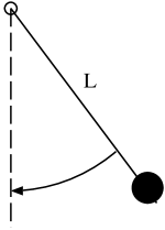
$\theta(t)$

Figure 2: The pendulum.

3 A typical example of simulation

We give on the figure 1 the skeleton of a simulation document. We will now explain with details how to build this document to describe a small simulation.

We consider the pendulum depicted on figure 2. We make the hypothesis that the line connecting the sphere of mass $M$ to the rotation axis is of negligible mass compared to $M$. We measure the deviation of the pendulum from the stable vertical equilibrium position by the angle $\theta(t)$ positively measured as indicated on figure 2. If one applies the relations of dynamics for bodies under rotations, we obtain the following ordinary differential equation

$$\left\{\begin{array}[]{rcl}\ddot{\theta}(t)&=&-\displaystyle\frac{g}{L}\sin\theta(t),\quad t\in[0,T]\\ \theta(0)&=&\theta_{0},\\ \dot{\theta}(0)&=&0.\end{array}\right.$$

The value of $\theta_{0}$ gives the initial angular deviation of the pendulum, and we consider that the initial angular velocity is zero. If $\theta_{0}$ is small, $\theta(t)$ can be approximated by $\phi(t)=\theta_{0}\cos\left(\sqrt{\frac{g}{L}}t\right)$. We want do describe a simulation applet allowing to compare $\phi(t)$ and $\theta(t)$ when $\theta_{0}$ changes. The graphical output should plot $\phi(t)$ and $\theta(t)$ for $t\in[0,T]$, and the user should have the possibility to change $\theta_{0}$ in the interval $[-3.14,3.14]$ by moving the point $(0,\theta_{0})$ interactively on the curve (the point will be represented with a cross). The XML code fragment containing the description of the parameters is given in figure 3.

⬇

1<parameters>

2 <section>

3 <title>Parameters of the pendulum</title>

4 <scalar label=”L” unit=”m”>

5 <name>Length of the pendulum</name>

6 <value>1</value>

7 </scalar>

8 <scalar label=”g0” unit=”ms^-2”>

9 <name>Gravity</name>

10 <value>9.81</value>

11 </scalar>

12 <point label=”point0”>

13 <x1 label=”zero”>

14 <value>0</value>

15 </x1>

16 <x2 label=”theta_0”>

17 <value>2</value>

18 </x2>

19 <constraints>

20 <curve ref=”segment”/>

21 </constraints>

22 </point>

23 </section>

24 <section>

25 <title>Resolution parameters</title>

26 <scalar label=”tf” unit=”s” min=”0” max=”10” increment=”1”>

27 <name>Final time</name>

28 <value>2</value>

29 </scalar>

30 </section>

31</parameters>

Figure 3: Code fragment containing the description of the parameters of the pendulum simulation

Each pair of section elements allows to group parameters. The scalar element represents a scalar parameter, containing its full name in the name element and its initial value in the element value. The constraint element refers to a curve with label segment, which will be described below. For the final simulation time, corresponding to the parameter with label tf (lines 26 to 29 in figure 3), there are bounds (minimum and maximum value) and also a relevant increment. During the compilation phase, the presence of these three attributes values will be taken into account and will allow to choose a particular widget in the graphical user interface.

3.1 Mathematical models, compute element

Here are the fragments corresponding to the description of the $[0,T]$ interval :

⬇

1<defdomain1d label=”t” unit=”s”>

2 <name>time</name>

3 <interval>

4 <initialvalue>0</initialvalue>

5 <finalvalue>tf</finalvalue>

6 </interval>

7</defdomain1d>

and the XML code fragment describing the differential equation is given in figure 4.

⬇

1<ode label=”pendulum”>

2 <refdomain1d ref=”t”/>

3 <states>

4 <state label=”theta” unit=”rad”>

5 <name>Real solution</name>

6 <derivative>theta_dot</derivative>

7 <initialcond>theta_0</initialcond>

8 </state>

9 <state label=”theta_dot” unit=”rad/s”>

10 <name>Derivative of the angle</name>

11 <derivative>-g0/L*sin(theta)</derivative>

12 <initialcond>0</initialcond>

13 </state>

14 </states>

15 <outputs>

16 <output label=”theta_lin”>

17 <name>Harmonic solution</name>

18 <value>theta_0*cos(sqrt(g0/L)*t)</value>

19 </output>

20 </outputs>

21</ode>

Figure 4: Code fragment containing the description of the system of two differential equations of the pendulum.

The ode element (ordinary differential equation) contains an empty element refdomain1d referring to the $[0,T]$ interval (defined earlier by the defdomain1d element, referred by the attribute ref), and thus defining the symbolic name of the integration variable, a states element containing the description of each state ($\theta$ and $\dot{\theta}$) in a state element. Each state element contains the name of the state, its time-derivative derivative and its initial value initialcond. Until now, the content of the derivative element is not parsed, and will copied verbatim during the compilation. Since we do not have a dedicated editor, this is easier for the user to type mathematical formulas like this, but we plan to use Content MathML (see e.g. [12]) in the future, which will allow an easier a priori validation of formulas.

The last element outputs in ode is a list of outputs, which can be functions of states and/or time. In our example the output explicitly depends on time but does not depend on the states. Each state or output has a mandatory attribute label which will be referred in the display section.

3.2 Graphs, curves and surfaces, graphs element

The code fragment describing the curve mentioned above is given in figure 5. We only need a simple segment connecting the points $(0,-3.14)$ and $(0,3.14)$. A point lying on this curve will have its ordinate in the interval $[-3.14,3.14]$. This curve will not be drawn as it only serves as a constraint for the value of $\theta_{0}$.

⬇

1<graphs>

2 <polyline label=”segment”>

3 <vertex x1=”0” x2=”-3.14”/>

4 <vertex x1=”0” x2=”3.14”/>

5 </polyline>

6</graphs>

Figure 5: Code fragment describing the segment joining the two points $(0,-3.14)$ and $(0,3.14)$.

It is not needed to write further XML code to construct the curves of $\theta(t)$ and $\phi(t)$ versus $t$, as it is possible to refer directly to the labels theta and theta_lin in the <drawcurve2d> element (see next section directly below).

3.3 Display of results, display element

We want to superimpose two curves in the same axes system, and display a movable cross at the $(0,\theta_{0})$ coordinate. The XML code corresponding to this is given in figure 6.

⬇

1<display>

2 <window>

3 <title>Comparison of the two solutions</title>

4 <axis2d>

5 <drawcurve2d ref=”theta”/>

6 <drawcurve2d ref=”thetalin”/>

7 <drawpoints ref=”point0”/>

8 </axis2d>

9 </window>

10<display>

Figure 6: Code fragment describing the display of the two solutions

The display element contains only one window element, containing itself a two dimensional system of axes. The two drawcurve2d elements within the same axis2d mean that the curves of $\theta$ and its harmonic version will be superimposed. The drawpoints element refers to the point element defined before in the parameters element.

3.4 Remarks

The different structuration possibilities are constrained by a DTD (Document Type Definition), allowing an a posteriori validation of a simulation, or can be used to constrain the edition of a simulation by means of an XML editor. The figure 7 shows the view that the user can have of its XML file.

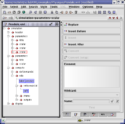
Figure 7: The XML file describing the simulation of the pendulum, seen in the XXE editor, developed by PIXWARE, http://www.xmlmind.com/xmleditor

Within all of the above mentioned elements, some have a particular status. The name and title elements can appear several times, with a different lang attribute (french or english in XMLlab 1.3). The goal is to be able to generate from the same XML file two different versions of the “compiled” applet, the language to use being specified as a compilation option.

The header element contains some meta-data such as the name of the author and some keywords. The notes element can appear several times with a different lang attribute and allows to write a few paragraphs of text allowing to describe the simulation and/or to give some help to the user.

4 The compilation chain

The compilation chain is entirely based on XML technologies: we use XSL transformations specified in XSL stylesheets (eXtensible Stylesheet Language). These transformations are applied to the simulation file by an “XSL processor”. The XSL technology is well known to allow the display of dynamic HTML on the World Wide Web, but it is also well fitted to the automatic generation of scripts. We are here particularly interested in the script language of Scilab or Matlab, and the script language Tcl/Tk, allowing to describe graphical user interfaces.

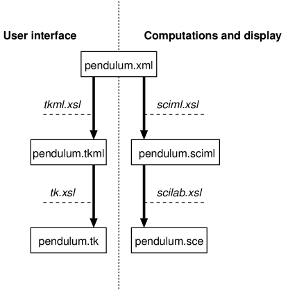
Figure 8: Diagram of the compilation chain. The arrows represent the XSL transformations, and the italic names the associated stylesheets.

The different phases of the compilation are outlined on the diagram depicted on figure 8. In the bottom of the diagram, the pendulum.sce file is the Scilab script containing all the computation code, and the display of results. The pendulum.tk file contains the Tcl/Tk code of the interface. The diagram illustrates the fact that the transformation is not direct and needs an intermediary step; this particular point needs an explanation.

To allow an easy maintenance of the XSL stylesheets, and especially to allow a smooth change of target languages (Scilab and Tcl/Tk), we have used “pivot” XML dialects: the code is generated in a two-step process. We use XSL transformation to translate XML input into a pseudo-Tcl/Tk and pseudo-Scilab syntax that are also written using XML dialects. Then we use a second pass to serialize the XML pseudo-language into the target language. The advantage here is that the second pass captures all the complexities of formatting clean code (syntax) while the first pass concentrates on the logical aspects of the translation (semantics). We use the following dialects :

• TKML dialect : as far as the interface Tcl/Tk code is concerned (left side of the diagram), the intermediary file pendulum.tkml is an XML file containing a logical description of the interface. This file contains the description of the different widgets (buttons, etc.) and their placement with respect to each other. Then, this intermediate file is finally translated in Tcl/Tk by means of a last XSL transformation.We show on figure 9 a small part of the generated markup. Almost all the parameters will be appear in the graphical user interface as classical entry widgets (corresponding to the “entry” widget in Tcl/Tk), where the user has to type the value with the keyboard keys. The <scale> element (lines 7 to 10 in figure 9) describes the widget which will be used for the final time of the simulation. Since the original markup describing this parameter in figure 3 gives bounds and an increment, the logical way of taking into account these constraints is to use a widget with a moving slider (in the final transformation we use the “scale” widget of Tcl/Tk). Some aspects of the TKML markup are very similar to the XForms markup language, which has been chosen by the W3C to develop the next generation of forms technology for the world wide web, see e.g. [13].

  ⬇

  1 <page name=”id66390” text=”Resolution␣parameters” pady=”4”>

  2 <frame packside=”top” anchor=”n” pady=”0” padx=”0” fill=”x” expand=”yes”>

  3 <frame packside=”left” padx=”5” expand=”true” fill=”x”>

  4 <label anchor=”w” expand=”true”>

  5 <text>Final time</text>

  6 </label>

  7 <scale anchor=”e” variable=”tf” state=”normal” width=”8” from=”1” to=”10” resolution=”1”>

  8 <value>2</value>

  9 <command>runScilab</command>

  10 </scale>

  11 </frame>

  12 </frame>

  13 </page>

  Figure 9: TKML intermediate markup corresponding to the definition of the Scilab function computing the right-hand side of the system of ordinary differential equations.

• SCIML dialect : for the Scilab code generation, we proceed in the same manner: we first generate an intermediary file pendulum.sciml, written using a pseudo-Scilab markup, and then transform this file to Scilab code with a last transformation. The figure 10 shows a fragment of the actual content of this file.

  ⬇

  1 <function-definition name=”f_pendulum”>

  2 <inputs>

  3 <parm>_t</parm>

  4 <parm>_X</parm>

  5 </inputs>

  6 <outputs>

  7 <parm>lhs</parm>

  8 </outputs>

  9 <body>

  10 <assign>

  11 <lhs>t</lhs>

  12 <rhs>_t</rhs>

  13 </assign>

  14 <assign>

  15 <lhs>theta</lhs>

  16 <rhs>

  17 <select matrix=”_X” row=”1:1” col=”1”/>

  18 </rhs>

  19 </assign>

  20 <assign>

  21 <lhs>theta_dot</lhs>

  22 <rhs>

  23 <select matrix=”_X” row=”2:2” col=”1”/>

  24 </rhs>

  25 </assign>

  26 <assign>

  27 <lhs>lhs</lhs>

  28 <rhs>

  29 <list sep=”;”>

  30 <parm>(theta_dot)</parm>

  31 <parm>(-g0/L*sin(theta))</parm>

  32 </list>

  33 </rhs>

  34 </assign>

  35 </body>

  36 </function-definition>

  Figure 10: SCIML intermediate markup corresponding to the definition of the Scilab function computing the right-hand side of the system of ordinary differential equations.

We show on figure 11 a small part of the generated Scilab script pendulum.sce appearing on figure 8, corresponding to the computation of the right-hand side of the first order differential equation obtained for the simulation of the pendulum, the call to the ode solver of Scilab and finally the display of curves (for sake of simplicity we have omitted some parts of the code).

⬇

1function [lhs]=f_pendulum(_t,_X)

2t=_t;

3theta=_X(1:1,1);

4theta_dot=_X(2:2,1);

5lhs=[(theta_dot);(-g0/L*sin(theta))];

6endfunction

7

8// Time

9t=linspace(0,tf,200)’;

10//␣Script␣code␣for␣the␣pendulum␣ode

11_X0(1:1,1)=theta_0;

12_X0(2:2,1)=0;

13_X=ode(_X0,0,t,f_pendulum);

14theta=_X(1:1,:)’;

15theta_dot=_X(2:2,:)’;

16thetalin=theta_0*cos(sqrt(g0/L)*t);

17

18//␣Display

19plot(t,theta,);

20hold(”on”);

21plot(t,thetalin,;

22hold(”off”);’

Figure 11: Some parts of the generated Scilab script for the pendulum simulation.

Two ways of distribution can be used: the two Tcl/Tk and Scilab files can be later used without using the XML source and the compilation chain (thus protecting the author’s work). However, it would be more profitable to the community to release the XML source.

The whole compilation chain together with Scilab (except the XML editor), uses only open-source software packages (xsltproc of the Gnome project, Tcl scripts), and works on any platform (Windows, Mac OS X, Unix).

5 The different ways of publishing an XMLlab simulation

In the previous section, we have described the classical way of publishing an XMLlab simulation, by using a “compilation chain” allowing to transform the original XML file pendulum.xml to a Scilab executable file pendulum.sce and a Tk file pendulum.tk which will be run on a local client machine where Scilab is installed. By using this kind of publication, the interactivity is maximal; for the pendulum example, the user can move the cross representing the initial condition and see in real time how the two trajectories diverge (see figure 13).

5.1 Comments on the example

5.1.1 Description of the generated graphical user interface

We make some comments on the figure 13.

• User interface : the window of the interface has a central space with a Notebook-type widget with tabs and a menu bar:

  • The two tabs named Parameters of the pendulum and Resolution parameters correspond to the two parameters groups specified in the XML file. The user just has to select a given tab to display the corresponding parameter group.

  • The Notes tab gives some some information on the simulation, extracted from the header element: name of the author, date and eventual notes describing the simulation. The XMLlab tab gives some information on the XMLlab project.

  • The File menu contains two interesting items: “Save a session” and “Load a session”. They allow to save the values of parameters in a text file, and to load them later. It allows to resume a working session (otherwise the Scilab script always starts with the initial values of parameters).

  • The Languages menu allows to switch between the languages of the simulation. In fact, by sake of simplicity we didn’t show the textual elements for each language in the pendulum example, but giving them in all desired languages allows to dynamically switch between languages when running a simulation. For example, when the default language (English here) and French are to be used, a typical code fragment is the one given in figure 12.

  ⬇

  1 <section>

  2 <title>Resolution parameters</title>

  3 <title lang=”french”>Paramètres de résolution</title>

  4 <scalar label=”T” unit=”s”>

  5 <name>Final time</name>

  6 <name lang=”french”>Temps final</name>

  7 <value>2</value>

  8 </scalar>

  9 </section>

  Figure 12: Code fragment showing textual elements in different languages.

• Graphical window : the legend of the two curves is taken from the name elements within the states theta and the output theta_lin. The abscissa label is the name of the time variable t, and the ordinate label is the unit (unit attribute of element <state label="theta"). This window belongs to Scilab, thus the user has access to the usual menus allowing to save (e.g. in EPS format) or print the figure.

The user has always the possibility to have access to all variables of the simulation from the Scilab command line (parameters and results of the simulation), which remains available during the simulation.

5.1.2 Remark on performances

For this particular example (a system of two scalar ordinary differential equations), the computation time is negligible compared to the time elapsed by drawing the curves, and hence the user can see the immediate effect of the initial angle on the synchronization of the curves. For more intensive examples (e.g. resolution of a partial differential equation), the response time can be greater, but the reactivity of the system is always good, even on a lightweight system (1Ghz Pentium). For these reasons Scilab is really appreciated, because the built-in functions are well optimized (linear and nonlinear equations solving, differential equations, sparse matrix algebra, vectorization of elementary functions for arrays, etc.). Moreover, Scilab loads in a negligible time (compared to the important startup time of recent versions of Matlab, because of the use of JAVA for the user interface).

$$\begin{array}[]{cc}\includegraphics[width=173.44534pt]{image2}&\leavevmode\nobreak\ \leavevmode\nobreak\ \includegraphics[width=173.44534pt]{image3}\\ \nobreak\leavevmode\hfil\\ \begin{minipage}[c]{173.44534pt}\includegraphics[width=173.44534pt]{image5}\end{minipage}&\leavevmode\nobreak\ \leavevmode\nobreak\ \begin{minipage}[c]{173.44534pt}\includegraphics[width=173.44534pt]{image6}\end{minipage}\\ \end{array}$$

Figure 13: Screenshots of the various tabs of the pendulum simulation running on a local client with Scilab. In the graphical window, the user can move the cross shaped pointer and see the trajectory changes in real time.

5.2 Offline batch publication of HTML pages

When a large number of simulations have to be deployed in an educational context, it is possible to automatically generate a tree of HTML files presenting the simulations e.g. sorted by categories. The HTML files, as well as some screenshots of the graphical output and of the user interface are automatically generated in a batch process which only takes a few minutes. The user can then browse the different pages, take a look at the screenshots, read the description and finally launch the chosen simulation. The typical HTML page for a single simulation is given on figure 14. Note: this kind of publication still needs Scilab on the client machines (see the examples section of the XMLlab WWW site [14]).

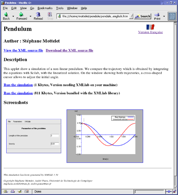
Figure 14: An HTML page describing the pendulum simulation. This kind of page is dedicated to serve the simulations to clients where Scilab is installed

5.3 Online distant publication using the XMLlab WebServer

Still in an educational context, but when it is not possible to have Scilab installed on all the client machines, it is possible to publish the simulation towards thin clients running a simple WWW browser. The drawbacks of such an approach are already known: there is an interactivity loss, but simulations can be deployed very fast.

We have chosen a rather classical architecture based on a HTTP server and the Common Gateway Interface. The entry point is a CGI script (written in Tcl) which processes the user requests (see figure 16). The collection of XML simulations to be served are stored in the server (running any flavor of Unix) and the only needed software is:

• Scilab with the XMLlab toolbox,

• An HTTP server, e.g. the Apache HTTP server,

• The VNC virtual X11 server,

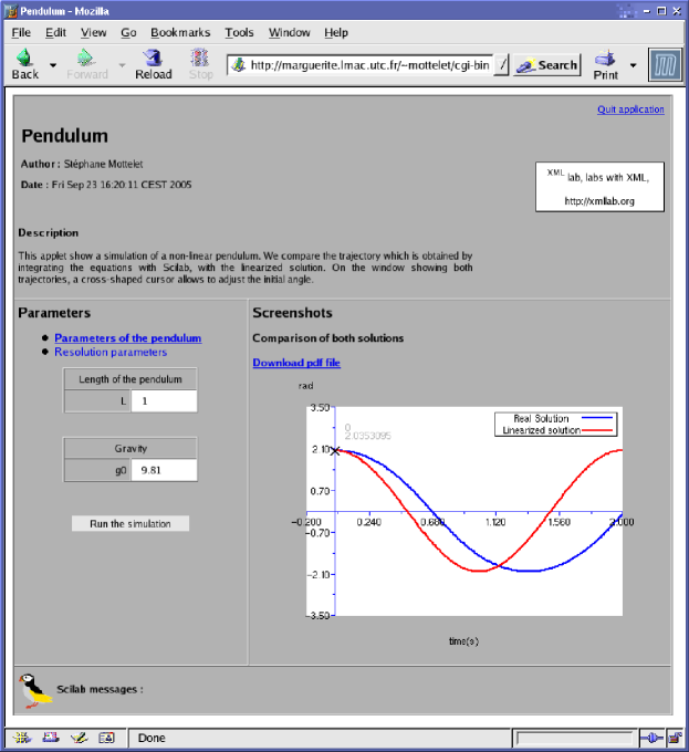
Figure 15: Screenshot of the pendulum simulation served by the XMLlab WebServer on a client machine running the Mozilla web browser on a Linux machine.

For the pendulum example, the generated HTML page can be seen on figure 15. The user can interact by changing the parameters values, browse the different parameter sections and download a PDF version of the graphical output.

We now describe how a typical URL (see on top of figure 16) is processed : when the first user request is processed, the CGI script associates a session number to the client and performs the following tasks :

1. Retrieve the XML file (here pendulum.xml) and process it in the XMLlab compilation chain. This produces two files, a Scilab file pendulum.sce (dedicated to computations and graphical output) and a Tk file pendulum.tk (dedicated to communications with the CGI script and HTML output).

2. Verify if the X11 VNC server is running (if not, a new server is launched), and launch a Scilab instance which uses this display for its graphical output.

3. Run pendulum.sce and pendulum.tk into Scilab. The obtained result is an HTML file pendulum.html together with image files corresponding with the first run of the simulation with default values of the parameters.

4. The HTML output is sent back to the client’s WWW browser.

The red arrows in figure 16 denote tasks which are only done at first user request. When the user interacts with the simulation, then parameter changes are sent to the simulation running into Scilab by using the Tk send mechanism.

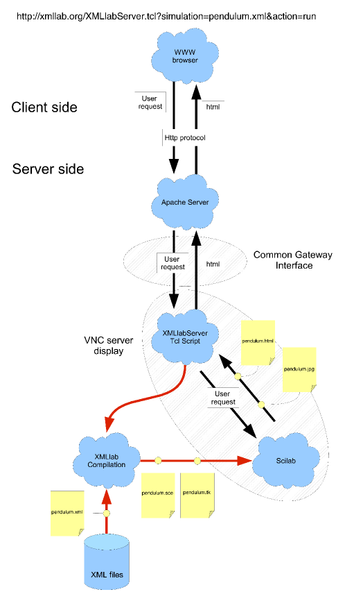
Figure 16: Internals of the XMLlab WebServer. Red arrows occur only at first user request.

6 Trends and conclusions

The different parameters types and the mathematical objects presented in section 2 are already present in XMLlab 1.6, but XMLlab is a work in constant progress, and many extensions and improvements are necessary. However, we think that the choices we have made are valid, especially concerning the structuring of the simulations and the architecture of the compilations chain. The needed development time to add a new type of equation is always limited: for example, the stationary-pde element, allowing to describe an elliptic partial differential equation (extension of the DTD and associated XSL stylesheet sections), has been developed in two days (we rely on a Scilab “PDE toolbox”).

The XMLlab WebServer allowing dynamic publication of the simulation towards thin clients is the most recent feature we have developed in XMLlab. Since we have opened the possibility to encapsulate Scilab scripts (making only computations) the XMLlab WebServer feature is giving to Scilab the equivalent of what the Matlab WebServer (this product is discontinued) used to provide to Matlab, but with a completely different approach, since the user doesn’t have to write any line of HTML. In this case, complex Scilab scripts, eventually computing some new values of the parameters (see e.g. the linear regression example in the Mathematics section of XMLlab  examples) are embedded in a script element, replacing the compute element. Of course all the other high level elements are present, and allow to do the same multi-medium publication as for pure XML simulation files (see e.g. the Discrete Cosine Transform and the Commutation Angles simulations in the examples).

The future developments of XMLlab mainly focus on, discrete time systems simulation, stochastic systems, generation of Adobe Flash animations, sound output, and so on. As far as the edition of the XML files is concerned, we plan to use “Cascading Stylesheets” allowing to edit XML files in a very user-friendly way in the XXE editor (see [15]). We also plan to migrate the actual DTD to an XML Schema ([16]), to allow some enhancements in the control of validity of the different data types contained in elements and attributes. In the current XMLlab release, this control is made in the XSL stylesheets.

At the time we are writing this paper, XMLlab has already been used for 3 years in chemistry courses at the UTC (150 students by semester), under the form of demonstrations during the course, and during the labs, together with experimental acid/alkali titrations. With the help of simulation the students interpret the experimental curves and are able to answer reasoning questions. The software is also available in the UTC intranet to allow students to improve their understanding of phenomenons. A sample survey has been made by e-mail at the end of each semester and allowed us to conclude that the software is easy to use, and students do not encounter major technical problems. The software allows a better understanding of complex phenomenon and acid/alkali equilibrium, but high level labs assistants are needed (they must be trained on the software before the labs). XMLlab is also used at the University Of Picardie Jules Verne since 2007, in the systems biology courses.

XMLlab has also been integrated in the prize-winning SCENARI Platform editorial chain (SCENARI Platform is an open source application suite for designing digital editing chains, used for creating professional standard multimedia documents, see [17, 18]).

Of course, many other examples of simulations have been written to show that XMLlab can be used in various disciplinary fields : we have examples in the fields of biology (microbial and enzymatic kinetics), physics (pendulum, oscillators, two-body system, Poisson equation, etc.), chemistry (Acid/Alkali equilibriums, chemical kinetics), chemical engineering (ideal reactors), etc. The complete list of available examples is given in appendix. All these simulations are available in French, English and Spanish, and the translation to German is in progress. We hope that a lot of people will contribute and request some new features, which will help us to make XMLlab fit to new disciplinary fields.

XMLlab is available at the address http://xmllab.org, as a Scilab toolbox under the GPL license. The distribution is available for all popular platforms (Windows, Linux, Solaris, Mac OS X) and well integrated, e.g. the applets can be run directly by double clicking the icon of the file, without having to launch Scilab before.

The documentation is available in French and English, under the form of a quick start guide and a reference manual.

XMLlab has been accepted as a contribution by the Scilab Consortium in June 2004, and one of the two authors is now an official contributor member of the Consortium, also sitting at the steering committee.

Appendix A List of the simulations examples available at the XMLlab WWW site: xmllab.org

• Image Processing

  • Discrete Cosine Transform.

• Engineering

  • Commutation angles.

• Physics

  • Damped Oscillator. Pendulum. Pendulum (with animation). Earth-Moon system. Simulation of the Laplace equation.

• Maths

  • Lissajous curve. A simple surface example. Tangent. Osculating polynomials. Gaussian mix. Lagrange Interpolation. Cycloïd. Linear regression. Inversion of a matrix. Helix. System of differential equations.

• Predation

  • Kinetics of prey predation by predators. Kinetics of rabbit predation by foxes.

• Chemical kinetics

  • Nonreversible reaction. Reversible reaction(equilibrium). Simultaneous reactions (in parallel). Successive reactions with an equilibrium.

• Enzymatic kinetics.

  • Enzymatic kinetics with a competitive inhibition. Enzymatic kinetics with a incompetitive inhibition. Enzymatic kinetics with a non-competitive inhibition. Michaelis-Menten’s enzymatic kinetics.

• Microbial kinetics

  • Graef-Andrews’s growth kinetics. Monod’s growth kinetics.

• pH titrations

  • Simulation of acid-alkali titration in water. Simulation of a single acid titration.

References

- [1] J.-P. Chancelier, F. Delebecque, C. Gomez, R. Goursat, M.and Nikoukah, S. Steer, Introduction à Scilab, Springer, Paris, 2001.
- [2] C. E. Gomez, Engineering and scientific computing with scilab, Birkauser, Boston, 1999.
- [3] P. Motta Pires, D. Rogers, Free/opensource software: an alternative of engineering students, Procceding of the 32nd ASEE/IEEE Frontiers in Education Conference, November 6 - 9.
- [4] T. Bray, J. Paoli, C. e. a. Sperberg-McQueen, Extensible markup language (xml) 1.0, Available via the World Wide Web at http://www.w3.org/TR/2004/REC-xml-20040204.
- [5] M. Hucka, A. Finney, H. Sauro, H. Bolouri, J. Doyle, al., The systems biology markup language (sbml): a medium for representation and exchange of biochemical netwok models, Bioinformatics 19 (2003) 524–531.
- [6] M. Hucka, A. Finney, Systems biology markup language: Level 2 and beyond, Biochem. Soc. Trans. 31 (2003) 1472–1473.
- [7] G. Collecutt, P. Drummond, J. Hope, P. Cochrane, Extensible multi-dimensional simulator (xmds), Available via the World Wide Web at http://www.physics.uq.edu.au/xmds/index.html.
- [8] W. Borutzky, a novel xml format for the exchange and the reuse of bond graph models of engineering systems, Simulation Modelling Practice and Theory 14 (2006) 787–808.
- [9] J. Ousterhout, Scripting: Higher-level programming for the 21st century, IEEE Computer magazine March (1998) 23–30.
- [10] J. Ousterhout, Tcl and the Tk toolkit, Addison-Wesley, 1994.
-
[11]
S. Mottelet, A. Pauss, Xmllab : un outil générique de simulation basé sur xml
et scilab, in: Proceedings of TICE 2004 conference, Université de Technologie
de Compiègne, [OAI : oai:edutice.archives-ouvertes.fr:edutice-00000726_v1] -
http:
//edutice.archives-ouvertes.fr/edutice-00000726, 2004, pp. 391–399. - [12] D. Carlisle, P. Ion, D. Miner, N. Poppelier, Mathematical markup language (mathml) version 2.0 (second edition) recommandation, Available via the World Wide Web at http://www.w3.org/TR/MathML.
- [13] J. Boyer, D. Landwher, R. Merrick, T. Raman, L. Dubinko, L. Klotz, Xforms 1.0 (second edition), Available via the World Wide Web at http://www.w3.org/TR/xforms.
- [14] S. Mottelet, A. Pauss, Xmllab web site, http://xmllab.org.
- [15] B. Bos, H. Wium Lie, C. Lilley, I. E. Jacobs, ascading stylesheets, level 2, css2 specification, Available via the World Wide Web at http://www.w3.org/TR/1998/REC-CSS2-19980512.
- [16] H. Thompson, D. Beech, M. Maloney, N. Mendelsohn, Xml schema part 1: Structures, Available via the World Wide Web at http://www.w3.org/TR/xmlschema-1.
- [17] B. Bachimont, I. Cailleau, M. Crozat, S.and Majada, S. Spinelli, Le procédé scenari : Une chaîne éditoriale pour la production de supports numériques de formation, in: Proceedings of TICE 2002 conference, INSA Lyon, 2002, pp. 183–192.
- [18] S. Crozat, S. Spinelli, Scenari paltform web site, http://scenari-platform.org/projects/scenari/en/pres/co/.
Acknowledgments
This work has been financed by the groupment “Evaluation of New Technologies in Education” of the regional Council of Research from Picardie and by the UNIT consortium (French Numeric University of Engineering and Technology). IUFM’s teachers and Jules Vernes University of Picardie Professors have contributed efficiently to the trandisciplinarity of this project.